A Screw Theory Approach to Computing the Instantaneous Rotation Centers of Indeterminate Planar Linkages

Abstract

This paper presents a screw theory approach for the computation of the instantaneous rotation centers of indeterminate planar linkages. Since the end of the 19th century, the determination of the instantaneous rotation, or velocity centers of planar mechanisms has been an important topic in kinematics that has led to the well-known Aronhold–Kennedy theorem. At the beginning of the 20th century, it was found that there were planar mechanisms for which the application of the Aronhold–Kennedy theorem was unable to find all the instantaneous rotation centers (IRCs). These mechanisms were denominated complex or indeterminate. The beginning of this century saw a renewed interest in complex or indeterminate planar mechanisms. In this contribution, a new and simpler screw theory approach for the determination of indeterminate rotation centers of planar linkages is presented. The new approach provides a simpler method for setting up the equations. Furthermore, the algebraic equations to be solved are simpler than the ones published to date. The method is based on the systematic application of screw theory, isomorphic to the Lie algebra, $se\left(3\right)$, of the Euclidean group, $SE\left(3\right)$, and the invariant symmetric bilinear forms defined on $se\left(3\right)$.

1. Introduction

The instantaneous rotation center (IRC) of two links in a one-DOF planar linkage is defined as a pair of coincident points that belong to each body and have the same velocity, with respect to another reference frame. Therefore, the relative motion between the two links is a rotation around an axis perpendicular to the plane of motion passing through the coincident points. Some IRCs can be easily determined by inspection. These IRCs are defined as primary. For example, each revolute pair constitutes the IRC of the two links that the revolute pair connects. If the IRC is not primary, then it is defined as secondary.

The Aronhold–Kennedy theorem was independently formulated by Aronhold [1], in Germany, and Kennedy [2], in England, in the second part of the 19th century. The Aronhold–Kennedy theorem is the main tool for determining secondary IRCs. The theorem indicates that the location of the IRCs associated with the relative movements of three arbitrary rigid bodies on the plane must be collinear. The great majority of planar linkages allow for the locating of all the IRCs of planar linkages using the Aronhold–Kennedy theorem. Therefore, for many decades, this theorem provided an efficient graphical method for the kinematic analysis of planar linkages; see Shigley and Uicker [3].

Nevertheless, since 1915, Klein [4] showed the existence of planar linkages for which the application of the Aronhold–Kennedy theorem was insufficient to determine the IRCs. These planar linkages were called complex planar linkages and, later, indeterminate planar linkages. Klein [4] proposed a graphical trial and error method for locating those IRCs that resisted the application of the Aronhold–Kennedy theorem.

In the middle of the 20th century, Modrey [5] employed influence coefficients to find the secondary IRCs of the so-called complex planar linkages. The posterior discussion by Goodman [6] is also quite illuminating. The method involves the solution of the velocity analysis of the indeterminate linkage and, from these results, it obtains the required IRCs. This approach reappeared in later dates, as in Yan et al. [7], and even in recent contributions, as in Kim et al. [8]. Nevertheless, in this latter case, the method was loosely applied—with many conceptual mistakes—to simple determinate planar linkages. Recently, Valderrama-Rodríguez et al. [9] generalized the approach for any spatial linkage and rebutted several statements presented in Kim et al. [8]. Moreover, from a historical point of view, the determination of the IRCs was employed precisely to carry out the velocity analysis of the linkages. In addition, the determination of the IRCs provides important insights on the performance of planar linkages, such as transmissibility, analysis of singularities (Di Gregorio [10]), and mechanical advantage (Zarkandi [11]), among others.

About 15 years ago, Pennock and Foster [12] presented a graphical technique that was able to find all the IRCs of indeterminate linkages and improved substantially the approach proposed by Klein. A few years later, Di Gregorio [13] introduced an analytical technique that generated a system of equations involving both the closure equations of the planar linkages and the location of the indeterminate IRCs, so that he was able to find the location of the indeterminate rotation centers. In 2009, Kung and Wang [14] employed graph theory to obtain a graph associated with the IRCs of a linkage. This graph allowed Kung and Wang to formulate a system of iterative equations, whose unknowns are the coordinates of the indeterminate IRCs. The solution of the problem comes down to solving a quadratic equation and then a quartic equation.

There is another line of research of the determination of the IRC of planar linkages. The origin of this line of research is due to Chang and Her [15], who in 2008 presented a virtual cam method for locating the IRCs of indeterminate linkages. This approach has been extended by Liu and Chang [16,17]. They extended the approach by introducing the “virtual cam–hexagon” method. They embarked themselves on the task of determining the IRCs of all indeterminate linkages, up to ten bar. It is important to note that the approach is almost completely graphical; Liu and Chang indicate that the [17] “…Virtual Cam–Hexagon Method is not a truly universal technique yet, but, at this moment all the other graphical and geometrical approaches are extremely limited which can only be applied on several specific constructions of kinematically indeterminate linkages, and all of those approaches either change the constructions of the original linkages dramatically, or some even alter the original system’s DOF. Virtual Cam–Hexagon Method does not change the construction of the original linkage, nor alter the system’s DOF in the procedure. With a nearly 75% success rate on all planar single DOF linkages up to ten-bar…”.

In this contribution, which follows a similar technique for indeterminate spherical linkages, Valderrama-Rodríguez et al. [18] introduced a more efficient approach than those presented previously for the determination of the IRCs of indeterminate spherical linkages. However, in the case of spherical linkages, only the Killing form is needed, whilst in the case of planar linkages, both the Killing and Klein forms are necessary. However, the influence of the Killing form is only recognized after the general analysis presented in this paper is carried out. Therefore, the analysis and application of both the Killing and Klein forms are required.

Some of the advantages of the method presented in this contribution are:

• The method requires a reduced set of equations. It will be shown that the development of the complete graph of the IRCs of the linkage, as proposed by Kung and Wang [14], is unnecessary. More specifically, by properly selecting a pair of sub-graphs of the complete graph, the determination of all secondary IRCs can be readily obtained;
• The required equations are simpler. The method presented by Di Gregorio [13] requires the solution of a nonlinear set of 10 equations, in one case, and a nonlinear set of 12 equations, in another case. The method presented by Kung and Wang [14] requires first the solution of a quadratic equation and, later, the solution of a quartic equation. The method presented in this contribution only requires the solution and comparison of 2 quadratic equations in one case, and a quadratic and a cubic equation in the other.

The rest of the contribution is revised in this paragraph. Section 2 presents the fundamental equation of the Aronhold–Kennedy theorem and the symmetric bilinear forms defined on, $se\left(3\right)$, the Lie algebra of the special Euclidean group, $SE\left(3\right)$, namely, the Killing and the Klein forms. The purpose of this section is two-fold. On the one hand, it shows that the application of the algebraic structure of the Lie algebra, $se\left(3\right)$, provides a unifying approach for the determination of the instantaneous screw axes of any spatial linkage; on the other hand, it shows that for planar linkages, the approach is reduced to the application of the Klein form to screws perpendicular to the plane motion—i.e., the classical Aronhold–Kennedy theorem. The importance of the Killing form has been obscured due to the history of kinematics, which for many decades was reduced to planar kinematics exclusively. Section 3 presents the complete approach for an eight-bar, partially indeterminate planar linkage. Section 4 solves an eight-bar, completely indeterminate planar linkage. Section 5 provides constructive proof for the validity of the method for all indeterminate linkages. Finally, some conclusions are drawn in Section 6. This paper contains a small Appendix A, which shows how to represent a secondary IRC as a linear combination of two primary IRCs.

2. The Fundamental Equation for the General Aronhold–Kennedy Theorem

This section starts with a definition of the velocity state of a body with respect to another body.

Definition 1.

Let j and m be a pair of different rigid bodies or reference frames, and let O be a point fixed in body m. The velocity state of body m with respect to body j is defined as

$${}^j{\mathbf{V}}_O^m\equiv \left[\begin{array}{c}{}^j{\mathbf{\omega }}^m\\ {}^j{\mathbf{v}}_O^m\end{array}\right]$$

(1)

where ${}^j{\mathbf{\omega }}^m$ is the angular velocity of body m with respect to body j, and ${}^j{\mathbf{v}}_O^m$ is the velocity of a point O, fixed to the rigid body m as observed from the rigid body j. Ball [19] defined ${}^j{\mathbf{V}}_O^m$ as a twist on a screw.

Proposition 1.

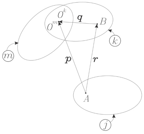
Let j, k, and m, be three different bodies or reference frames, see Figure 1, and let ${}^j{\mathbf{V}}_O^k$, ${}^j{\mathbf{V}}_O^m$, and ${}^k{\mathbf{V}}_O^m$ be their corresponding velocity states, as given by Definition 1. Then:

$${}^j{\mathbf{V}}_O^m={}^j{\mathbf{V}}_O^k+{}^k{\mathbf{V}}_O^m$$

or

$$\begin{array}{ccc}\hfill \left[\begin{array}{c}{}^j{\mathbf{\omega }}^m\\ {}^j{\mathbf{v}}_O^m\end{array}\right]& =& \left[\begin{array}{c}{}^j{\mathbf{\omega }}^k\\ {}^j{\mathbf{v}}_O^k\end{array}\right]+\left[\begin{array}{c}{}^k{\mathbf{\omega }}^m\\ {}^k{\mathbf{v}}_O^m\end{array}\right]\hfill \end{array}$$

(2)

Figure 1. Three rigid bodies and the related points and vectors.

It is important to note that Equation (2) is valid whether the bodies are connected via kinematic pairs or are unconnected. This result is presented in Rico et al. [20], but it is quite likely that it was well known from the beginning of the last century, and that Ball [19] was aware of its meaning, despite not using the vector notation.

In the Lie algebra $se\left(3\right)$ of the Euclidean group $SE\left(3\right)$, two invariant symmetrical bilinear forms can be defined.

Definition 2.

Consider the Lie algebra, $se\left(3\right)$, of the Euclidean group, $SE\left(3\right)$. Then, it is possible to define a bilinear symmetric form, denoted as the Killing form for any screws ${\mathbf{V}}_{O1}$, ${\mathbf{V}}_{O2}\in se\left(3\right)$, as follows:

$$Ki:se\left(3\right)\times se\left(3\right)\to \mathbf{R}Ki({\mathbf{V}}_{O1},{\mathbf{V}}_{O2})=Ki\left(({\mathbf{\omega }}_1;{\mathbf{v}}_{O1}),({\mathbf{\omega }}_2;{\mathbf{v}}_{O2})\right)={\mathbf{\omega }}_1·{\mathbf{\omega }}_2$$

where “·” is the scalar product of three-dimensional vector algebra.

Definition 3.

Consider the Lie algebra, $se\left(3\right)$, of the Euclidean group, $SE\left(3\right)$. Then, it is possible to define a bilinear symmetric form, denoted as the Klein form, for any screws ${\mathbf{V}}_{O1}$, ${\mathbf{V}}_{O2}\in se\left(3\right)$, as follows:

$$Kl:se\left(3\right)\times se\left(3\right)\to \mathbf{R}Kl({\mathbf{V}}_{O1},{\mathbf{V}}_{O2})=Kl\left(({\mathbf{\omega }}_1;{\mathbf{v}}_{O1}),({\mathbf{\omega }}_2;{\mathbf{v}}_{O2})\right)={\mathbf{\omega }}_1·{\mathbf{v}}_{O2}+{\mathbf{\omega }}_2·{\mathbf{v}}_{O1}$$

where "·" is the scalar product of three-dimensional vector algebra. This symmetric bilinear form is also called the reciprocal product of the screws.

It can be proved that both symmetrical bilinear forms, Killing and Klein, are well defined or invariant, i.e., the result is independent of the point O used to determine the velocity state or the selection of the coordinate system; see, for example, Brand [21], although the reader is cautioned that Brand used the “motor” terminology for screws. Moreover, it can be proved that the Klein form is a nonsingular indefinite symmetric bilinear form on $se\left(3\right)$, while the Killing form is a singular positive semi-definite symmetric bilinear form on $se\left(3\right)$ (Rico and Duffy [22]).

Finally, given a screw $, any screw ${\$}_a$ that satisfies $Ki(\$,{\$}_a)=0$ is called an orthogonal annihilator, regarding the Killing form of the original screw $. It should be noted that, if $Ki(\$,{\$}_a)=0$, the direction of the axes of the screws are perpendicular. Similarly, any screw ${\$}_a$ that satisfies $Kl(\$,{\$}_a)=0$ is called an orthogonal annihilator, regarding the Klein form of the original screw $; frequently, the screw ${\$}_a$, in this latter case, is also called the reciprocal screw of the original screw $.

Symbolically, Equation (2) can be written as:

$${}_j{\omega }_m{}^j{\$}^m={}^j{\mathbf{V}}_O^m={}^j{\mathbf{V}}_O^k+{}^k{\mathbf{V}}_O^m={}_j{\omega }_k{}^j{\$}^k+{}_k{\omega }_m{}^k{\$}^m$$

(3)

where the infinitesimal screw, let us say, ${}^j{\$}^m$, is given by:

$${}^j{\$}^m=\left[\begin{array}{c}{}^j{\mathbf{u}}^m\\ {}^j{\mathbf{r}}^m\times {}^j{\mathbf{u}}^m+{}_{j}h{}_m{}^j{\mathbf{u}}^m\end{array}\right]$$

(4)

with ${}^j{\mathbf{u}}^m$ being a corresponding unit vector in the direction of the screw axis, ${}^j{\mathbf{r}}^m$ is the position vector of a point along the screw axis, about the origin of the coordinate system, ${}_{j}h{}_m$ is the pitch of the screw, and “×” is the vector product of three-dimensional vector algebra.

The determination of an instantaneous screw axis, for example, ${}^j{\$}^m$, requires the orthogonal annihilators, regarding the Klein and Killing forms, of the subspace of $se\left(3\right)$ generated by $\{{}^j{\$}^k,{}^k{\$}^m\}$, denoted also as $\left[{}^j{\$}^k,{}^k{\$}^m\right]$. (This notation should not be confused with the Lie product, which in this contribution does not play any role.) Therefore, we will look for those screws ${\$}_{ajm}$ that:

• are orthogonal concerning the Klein form (also called reciprocal):

  $$Kl({\$}_{ajm},{}^j{\$}^k)=Kl({\$}_{ajm},{}^k{\$}^m)=0;$$

  (5)
• are orthogonal regarding the Killing form (also called perpendicular):

  $$Ki({\$}_{ajm},{}^j{\$}^k)=Ki({\$}_{ajm},{}^k{\$}^m)=0.$$

  (6)

Therefore, for the Klein and Killing forms, one has:

$$\begin{array}{ccc}\hfill Kl({\$}_{ajm},{}_j{\omega }_m{}^j{\$}^m)& =& Kl({\$}_{ajm},{}^j{\mathbf{V}}_O^m)=Kl({\$}_{ajm},{}^j{\mathbf{V}}_O^k+{}^k{\mathbf{V}}_O^m)\hfill \\ \hfill & =& Kl({\$}_{ajm},{}_j{\omega }_k{}^j{\$}^k+{}_k{\omega }_m{}^k{\$}^m)\hfill \\ \hfill & =& {}_j{\omega }_{k}Kl({\$}_{ajm},{}^j{\$}^k)+{}_k{\omega }_{m}Kl({\$}_{ajm},{}^k{\$}^m)={}_j{\omega }_k\left(0\right)+{}_k{\omega }_m\left(0\right)=0\hfill \end{array}$$

(7)

and

$$\begin{array}{ccc}\hfill Ki({\$}_{ajm},{}_j{\omega }_m{}^j{\$}^m)& =& Ki({\$}_{ajm},{}^j{\mathbf{V}}_O^m)=Ki({\$}_{ajm},{}^j{\mathbf{V}}_O^k+{}^k{\mathbf{V}}_O^m)\hfill \\ \hfill & =& Ki({\$}_{ajm},{}_j{\omega }_k{}^j{\$}^k+{}_k{\omega }_m{}^k{\$}^m)\hfill \\ \hfill & =& {}_j{\omega }_{k}Ki({\$}_{ajm},{}^j{\$}^k)+{}_k{\omega }_{m}Ki({\$}_{ajm},{}^k{\$}^m)={}_j{\omega }_k\left(0\right)+{}_k{\omega }_m\left(0\right)=0\hfill \end{array}$$

(8)

Summarizing, one may conclude that the orthogonal annihilators of the subspace generated for $\{{}^j{\$}^k,{}^k{\$}^m\}$ annihilate also the screw ${}^j{\$}^m$ associated with the instantaneous screw axis of the relative movement between links j and m. These two Equations (7) and (8), are the fundamental equations of the Aronhold–Kennedy theorem for general spatial linkages.

2.1. The Simplification for Planar Linkages

It is important to note that the role of the Klein and Killing forms can be drastically simplified if the linkages to be analyzed are planar. Without loss of generality, it will be assumed that the common plane of motion is perpendicular to the Z-axis. In planar linkages, kinematic pairs can be revolute or prismatic joints. The axes of the revolute pairs are all parallel to the Z-axis, while the directions of prismatic pairs must be perpendicular to the Z-axis; therefore, the screws representing revolute and prismatic pairs, Equation (4), can be, respectively, reduced as:

$${}^j{\$}^m=\left[\begin{array}{c}\mathbf{k}\\ {}^j{\mathbf{r}}^m\times \mathbf{k}\end{array}\right],\mathrm{a}\mathrm{n}\mathrm{d}{}^n{\$}^r=\left[\begin{array}{c}\mathbf{0}\\ {}^n{\mathbf{u}}^r\end{array}\right],\mathrm{w}\mathrm{h}\mathrm{e}\mathrm{r}\mathrm{e}{}^n{\mathbf{u}}^r·\mathbf{k}=0.$$

(9)

Without loss of generality, it can be assumed that $\mathbf{k}·{}^j{\mathbf{r}}^m=0$, for any ${}^j{\mathbf{r}}^m$, i.e., ${}^j{\mathbf{r}}^m$ and $\mathbf{k}$, are perpendicular.

It follows that, for planar linkages, the corresponding Lie algebra is not $se\left(3\right)$, but the subalgebra $g_{\mathbf{k}}$ is also denominated $se\left(2\right)$. This is the Lie subalgebra associated with the planar displacement subgroup, $G_{\mathbf{k}}$; it is also called the planar subgroup. Furthermore, $g_{\mathbf{k}}$ continues to be an orthogonal space under the restrictions of the Klein and Killing forms to $g_{\mathbf{k}}$ itself. However, the restricted Klein and Killing forms, in $g_{\mathbf{k}}$, have properties that are different from those in $se\left(3\right)$.

The Killing form for any pair of screws, ${}^j{\$}^m$ and ${}^n{\$}^r$, associated with the revolute pairs of any planar linkage, becomes

$$\begin{array}{ccc}\hfill Ki& :& g_{\mathbf{k}}\times g_{\mathbf{k}}\to \mathbf{R}Ki({}^j{\$}^m,{}^n{\$}^r)=Ki\left(\left[\begin{array}{c}\mathbf{k}\\ {}^j{\mathbf{r}}^m\times \mathbf{k}\end{array}\right],\left[\begin{array}{c}\mathbf{k}\\ {}^n{\mathbf{r}}^r\times \mathbf{k}\end{array}\right]\right)=\mathbf{k}·\mathbf{k}=1.\hfill \end{array}$$

(10)

If one of the screws, namely, ${}^j{\$}^m$, represents a prismatic pair, it follows that:

$$\begin{array}{ccc}\hfill Ki& :& g_{\mathbf{k}}\times g_{\mathbf{k}}\to \mathbf{R}Ki({}^j{\$}^m,{}^n{\$}^r)=Ki\left(\left[\begin{array}{c}\mathbf{0}\\ {}^j{\mathbf{u}}^m\end{array}\right],\left[\begin{array}{c}\mathbf{k}\\ {}^n{\mathbf{r}}^r\times \mathbf{k}\end{array}\right]\right)=\mathbf{0}·\mathbf{k}=0.\hfill \end{array}$$

(11)

In the language of orthogonal spaces, the restriction of the Killing form to the subalgebra $g_{\mathbf{k}}$ becomes a singular symmetric bilinear form.

Similarly, the Klein form for any pair of screws, ${}^j{\$}^m$ and ${}^n{\$}^r$, associated with the revolute pairs of any planar linkage, becomes:

$$\begin{array}{ccc}\hfill Kl& :& g_{\mathbf{k}}\times g_{\mathbf{k}}\to \mathbf{R}Kl({}^j{\$}^m,{}^n{\$}^r)=Kl\left(\left[\begin{array}{c}\mathbf{k}\\ {}^j{\mathbf{r}}^m\times \mathbf{k}\end{array}\right],\left[\begin{array}{c}\mathbf{k}\\ {}^n{\mathbf{r}}^r\times \mathbf{k}\end{array}\right]\right)\hfill \\ \hfill & & =\mathbf{k}·({}^n{\mathbf{r}}^r\times \mathbf{k})+\mathbf{k}·({}^j{\mathbf{r}}^m\times \mathbf{k})=0\hfill \end{array}$$

(12)

for any ${}^j{\$}^m,{}^n{\$}^r\in g_{\mathbf{k}}$. This result is consistent with a well-known result in screw theory that states that any pair of parallel 0-pitch screws are reciprocal, i.e., they are orthogonal regarding the Klein form.

If one of the screws, namely, ${}^j{\$}^m$, represents a prismatic pair, it follows that:

$$\begin{array}{ccc}\hfill Kl& :& g_{\mathbf{k}}\times g_{\mathbf{k}}\to \mathbf{R}Kl({}^j{\$}^m,{}^n{\$}^r)=Kl\left(\left[\begin{array}{c}\mathbf{0}\\ {}^j{\mathbf{u}}^m\end{array}\right],\left[\begin{array}{c}\mathbf{k}\\ {}^n{\mathbf{r}}^r\times \mathbf{k}\end{array}\right]\right)\hfill \\ \hfill & & =\mathbf{0}·({}^n{\mathbf{r}}^r\times \mathbf{k})+\mathbf{k}·{}^j{\mathbf{u}}^m=0+0=0.\hfill \end{array}$$

(13)

Thus, the restriction of the Klein form to the subalgebra $g_{\mathbf{k}}$ becomes also a lsingular symmetric bilinear form.

2.2. Application of the Killing and Klein Forms to Planar Linkages

This section shows the detailed process to obtain the equations that allow determining the secondary centers using the Aronhold–Kennedy theorem, as it was outlined in Equations (7) and (8).

Consider a pair of screws associated with a revolute joint and a prismatic joint of a planar linkage, as shown in Equation (9), repeated here:

$${}^j{\$}^m=\left[\begin{array}{c}\mathbf{k}\\ {}^j{\mathbf{r}}^m\times \mathbf{k}\end{array}\right]{}^n{\$}^r=\left[\begin{array}{c}\mathbf{0}\\ {}^n{\mathbf{u}}^r\end{array}\right],\mathrm{with}{}^n{\mathbf{u}}^r·\mathbf{k}=0$$

As indicated previously, without loss of generality, it will be assumed that the common plane of displacements is perpendicular to the Z-axis. Therefore, the axes of the revolute pairs are all parallel to the Z-axis, while the directions of the prismatic pairs must be perpendicular to the Z-axis. Additionally, without loss of generality, it can be assumed that $\mathbf{k}·{}^j{\mathbf{r}}^m=0$, namely, ${}^j{\mathbf{r}}^m$ and $\mathbf{k}$, are perpendicular. Moreover, the vector ${}^j{\mathbf{r}}^m$ provides the location of the instantaneous rotation, or velocity center represented by ${}^j{\$}^m$. The process must consider two cases.

First Case. The two kinematic pairs are revolute joints. Consider a subspace of $g_{\mathbf{k}}$, given by $\left[{}^j{\$}^m,{}^n{\$}^r\right]$, where:

$${}^j{\$}^m=\left[\begin{array}{c}\mathbf{k}\\ {}^j{\mathbf{r}}^m\times \mathbf{k}\end{array}\right]\mathrm{and}{}^n{\$}^r=\left[\begin{array}{c}\mathbf{k}\\ {}^n{\mathbf{r}}^r\times \mathbf{k}\end{array}\right].$$

Let

$${\$}_a=\left[\begin{array}{c}\mathbf{u}\\ {\mathbf{r}}_a\times \mathbf{u}\end{array}\right]$$

be an orthogonal annihilator of the subspace $\left[{}^j{\$}^m,{}^n{\$}^r\right]$ regarding both the Killing and Klein forms. Then:

1. applying the Killing form, it follows that:

$$\begin{array}{ccc}\hfill Ki({\$}_a,{}^j{\$}^m)& =& Ki\left(\left[\begin{array}{c}\mathbf{u}\\ {\mathbf{r}}_a\times \mathbf{u}\end{array}\right],\left[\begin{array}{c}\mathbf{k}\\ {}^j{\mathbf{r}}^m\times \mathbf{k}\end{array}\right]\right)=\mathbf{u}·\mathbf{k}=0\hfill \\ \hfill Ki({\$}_a,{}^n{\$}^r)& =& Ki\left(\left[\begin{array}{c}\mathbf{u}\\ {\mathbf{r}}_a\times \mathbf{u}\end{array}\right],\left[\begin{array}{c}\mathbf{k}\\ {}^n{\mathbf{r}}^r\times \mathbf{k}\end{array}\right]\right)=\mathbf{u}·\mathbf{k}=0\hfill \end{array}$$

Therefore, $\mathbf{u}$ and $\mathbf{k}$ must be perpendicular. Hence, $\mathbf{u}$ must be of the form $\mathbf{u}=u_x\mathbf{i}+u_y\mathbf{j}$ and, without loss of generality, it will be assumed that ${\mathbf{r}}_a=r_{ax}\mathbf{i}+r_{ay}\mathbf{j}$. Therefore, ${\$}_a$, the orthogonal annihilator of the subspace $\left[{}^j{\$}^m,{}^n{\$}^r\right]$ regarding the Killing form, is given by:

$${\$}_a=\left[\begin{array}{c}\mathbf{u}\\ {\mathbf{r}}_a\times \mathbf{u}\end{array}\right]=\left[\begin{array}{c}{u}_x\mathbf{i}+u_y\mathbf{j}\\ (r_{ax}\mathbf{i}+r_{ay}\mathbf{j})\times (u_x\mathbf{i}+u_y\mathbf{j})\end{array}\right];$$

2. applying the Klein form, it follows that:

$$Kl({\$}_a,{}^j{\$}^m)=Kl\left(\left[\begin{array}{c}\mathbf{u}\\ {\mathbf{r}}_a\times \mathbf{u}\end{array}\right],\left[\begin{array}{c}\mathbf{k}\\ {}^j{\mathbf{r}}^m\times \mathbf{k}\end{array}\right]\right)=\mathbf{u}·\left({}^j{\mathbf{r}}^m\times \mathbf{k}\right)+\mathbf{k}·\left({\mathbf{r}}_a\times \mathbf{u}\right)=0$$

(14)

$$Kl({\$}_a,{}^n{\$}^r)=Kl\left(\left[\begin{array}{c}\mathbf{u}\\ {\mathbf{r}}_a\times \mathbf{u}\end{array}\right],\left[\begin{array}{c}\mathbf{k}\\ {}^n{\mathbf{r}}^r\times \mathbf{k}\end{array}\right]\right)=\mathbf{u}·\left({}^n{\mathbf{r}}^r\times \mathbf{k}\right)+\mathbf{k}·\left({\mathbf{r}}_a\times \mathbf{u}\right)=0$$

(15)

Using the identities of the scalar triple product on Equations (14) and (15), one obtains:

$$\begin{array}{ccc}\hfill 0& =& \mathbf{u}·\left({}^j{\mathbf{r}}^m\times \mathbf{k}\right)+\mathbf{k}·\left({\mathbf{r}}_a\times \mathbf{u}\right)=\mathbf{k}·\left(\mathbf{u}\times {}^j{\mathbf{r}}^m\right)+\mathbf{u}·\left(\mathbf{k}\times {\mathbf{r}}_a\right)\hfill \\ \hfill & =& {}^j{\mathbf{r}}^m·\left(\mathbf{k}\times \mathbf{u}\right)+{\mathbf{r}}_a·\left(\mathbf{u}\times \mathbf{k}\right)=({}^j{\mathbf{r}}^m-{\mathbf{r}}_a)·\left(\mathbf{k}\times \mathbf{u}\right)\hfill \end{array}$$

(16)

and

$$\begin{array}{ccc}\hfill 0& =& \mathbf{u}·\left({}^n{\mathbf{r}}^r\times \mathbf{k}\right)+\mathbf{k}·\left({\mathbf{r}}_a\times \mathbf{u}\right)=\mathbf{k}·\left(\mathbf{u}\times {}^n{\mathbf{r}}^r\right)+\mathbf{u}·\left(\mathbf{k}\times {\mathbf{r}}_a\right)\hfill \\ \hfill & =& {}^n{\mathbf{r}}^r·\left(\mathbf{k}\times \mathbf{u}\right)+{\mathbf{r}}_a·\left(\mathbf{u}\times \mathbf{k}\right)=({}^n{\mathbf{r}}^r-{\mathbf{r}}_a)·\left(\mathbf{k}\times \mathbf{u}\right)\hfill \end{array}$$

(17)

Denoting, by $\mathbf{k}\times \mathbf{u}={\mathbf{u}}^{\perp }$, a unit vector perpendicular to both $\mathbf{u}$ and $\mathbf{k}$, and therefore in the X–Y plane, Equations (16) and (17) can be written as:

$${}^j{\mathbf{r}}^m·{\mathbf{u}}^{\perp }={}^n{\mathbf{r}}^r·{\mathbf{u}}^{\perp }={\mathbf{r}}_a·{\mathbf{u}}^{\perp }\mathrm{or}\left({}^j{\mathbf{r}}^m-{}^n{\mathbf{r}}^r\right)·{\mathbf{u}}^{\perp }=0$$

(18)

Equation (18) indicates that ${}^j{\mathbf{r}}^m-{}^n{\mathbf{r}}^r$ is perpendicular to ${\mathbf{u}}^{\perp }$. Since $\mathbf{u}$ and ${\mathbf{u}}^{\perp }$ must lie in the X–Y plane; then:

$${\left({\mathbf{u}}^{\perp }\right)}^{\perp }=\mathbf{u}$$

Therefore, ${}^j{\mathbf{r}}^m-{}^n{\mathbf{r}}^r$ must be parallel to $\mathbf{u}$; consequently:

$${}^j{\mathbf{r}}^m-{}^n{\mathbf{r}}^r=\lambda \mathbf{u}$$

(19)

Equations (15), (16) and (19) indicate that the orthogonal annihilator ${\$}_a$ must lay in the X–Y plane and intersect with both ${}^j{\$}^m$ and ${}^n{\$}^r$. Hence, the following proposition has been proved:

Proposition 2.

Let ${}^j{\$}^m$ and ${}^n{\$}^r$ be the screws representing a pair of revolute pairs whose common direction is the Z-axis, and let ${}^j{\mathbf{r}}^m$ and ${}^n{\mathbf{r}}^r$ be the position vectors of two points in the X–Y plane along the corresponding screw axis. Then, the orthogonal annihilator ${\$}_a$ must lie in the X–Y plane, and it must pass through ${}^j{\mathbf{r}}^m$ and ${}^n{\mathbf{r}}^r$.

Second Case. One kinematic pair is a revolute joint, the other is a prismatic joint. Consider a subspace of $g_{\mathbf{k}}$, given by $\left[{}^j{\$}^m,{}^n{\$}^r\right]$:

$${}^j{\$}^m=\left[\begin{array}{c}\mathbf{k}\\ {}^j{\mathbf{r}}^m\times \mathbf{k}\end{array}\right]\mathrm{and}{}^n{\$}^r=\left[\begin{array}{c}\mathbf{0}\\ {}^n{\mathbf{u}}^r\end{array}\right]$$

where ${}^n{\mathbf{u}}^r$ lies on the X–Y plane. Let

$${\$}_a=\left[\begin{array}{c}\mathbf{u}\\ {\mathbf{r}}_a\times \mathbf{u}\end{array}\right]$$

be an orthogonal annihilator of the subspace $\left[{}^j{\$}^m,{}^n{\$}^r\right]$ regarding both the Killing and Klein forms. Then:

1. applying the Killing form, it follows that:

$$\begin{array}{ccc}\hfill Ki({\$}_a,{}^j{\$}^m)& =& Ki\left(\left[\begin{array}{c}\mathbf{u}\\ {\mathbf{r}}_a\times \mathbf{u}\end{array}\right],\left[\begin{array}{c}\mathbf{k}\\ {}^j{\mathbf{r}}^m\times \mathbf{k}\end{array}\right]\right)=\mathbf{u}·\mathbf{k}=0\hfill \\ \hfill Ki({\$}_a,{}^n{\$}^r)& =& Ki\left(\left[\begin{array}{c}\mathbf{u}\\ {\mathbf{r}}_a\times \mathbf{u}\end{array}\right],\left[\begin{array}{c}\mathbf{0}\\ {}^n{\mathbf{u}}^r\end{array}\right]\right)=\mathbf{u}·\mathbf{0}=0\hfill \end{array}$$

Therefore, $\mathbf{u}$ and $\mathbf{k}$ must be perpendicular. Hence, $\mathbf{u}$ must be of the form $\mathbf{u}=u_x\mathbf{i}+u_y\mathbf{j}$ and, without loss of generality, it will be assumed that ${\mathbf{r}}_a=r_{ax}\mathbf{i}+r_{ay}\mathbf{j}$. Therefore, ${\$}_a$, the orthogonal annihilator of the subspace $\left[{}^j{\$}^m,{}^n{\$}^r\right]$ regarding the Killing form, is given by:

$${\$}_a=\left[\begin{array}{c}\mathbf{u}\\ {\mathbf{r}}_a\times \mathbf{u}\end{array}\right]=\left[\begin{array}{c}{u}_x\mathbf{i}+u_y\mathbf{j}\\ (r_{ax}\mathbf{i}+r_{ay}\mathbf{j})\times (u_x\mathbf{i}+u_y\mathbf{j})\end{array}\right];$$

2. applying the Klein form, it follows that:

$$\begin{array}{ccc}\hfill Kl({\$}_a,{}^j{\$}^m)& =& Kl\left(\left[\begin{array}{c}\mathbf{u}\\ {\mathbf{r}}_a\times \mathbf{u}\end{array}\right],\left[\begin{array}{c}\mathbf{k}\\ {}^j{\mathbf{r}}^m\times \mathbf{k}\end{array}\right]\right)=\mathbf{u}·\left({}^j{\mathbf{r}}^m\times \mathbf{k}\right)+\mathbf{k}·\left({\mathbf{r}}_a\times \mathbf{u}\right)=0\hfill \end{array}$$

(20)

Using the identities of the scalar triple product on Equation (20), it yields:

$$\begin{array}{ccc}\hfill 0& =& \mathbf{u}·\left({}^j{\mathbf{r}}^m\times \mathbf{k}\right)+\mathbf{k}·\left({\mathbf{r}}_a\times \mathbf{u}\right)=\mathbf{k}·\left(\mathbf{u}\times {}^j{\mathbf{r}}^m\right)+\mathbf{u}·\left(\mathbf{k}\times {\mathbf{r}}_a\right)\hfill \\ \hfill & =& {}^j{\mathbf{r}}^m·\left(\mathbf{k}\times \mathbf{u}\right)+{\mathbf{r}}_a·\left(\mathbf{u}\times \mathbf{k}\right)=({}^j{\mathbf{r}}^m-{\mathbf{r}}_a)·\left(\mathbf{k}\times \mathbf{u}\right)\hfill \end{array}$$

(21)

Denoting, by $\mathbf{k}\times \mathbf{u}={\mathbf{u}}^{\perp }$, a unit vector perpendicular to both $\mathbf{u}$ and $\mathbf{k}$, and therefore in the X–Y plane, Equation (21) can be written as:

$${}^j{\mathbf{r}}^m·{\mathbf{u}}^{\perp }={\mathbf{r}}_a·{\mathbf{u}}^{\perp }\mathrm{or}\left({}^j{\mathbf{r}}^m-{\mathbf{r}}_a\right)·{\mathbf{u}}^{\perp }=0$$

(22)

Equation (22) indicates that ${}^j{\mathbf{r}}^m-{\mathbf{r}}_a$ is perpendicular to ${\mathbf{u}}^{\perp }$. Since $\mathbf{u}$ and ${\mathbf{u}}^{\perp }$ must lie in the X–Y plane, then:

$${\left({\mathbf{u}}^{\perp }\right)}^{\perp }=\mathbf{u}$$

Therefore, ${}^j{\mathbf{r}}^m-{\mathbf{r}}_a$ must be parallel to $\mathbf{u}$; consequently:

$${}^j{\mathbf{r}}^m-{\mathbf{r}}_a=\lambda \mathbf{u}\mathrm{or}{}^j{\mathbf{r}}^m={\mathbf{r}}_a+\lambda \mathbf{u}$$

(23)

and

$$\begin{array}{ccc}\hfill Kl({\$}_a,{}^n{\$}^r)& =& Kl\left(\left[\begin{array}{c}\mathbf{u}\\ {\mathbf{r}}_a\times \mathbf{u}\end{array}\right],\left[\begin{array}{c}\mathbf{0}\\ {}^n{\mathbf{u}}^r\end{array}\right]\right)=\mathbf{u}·{}^n{\mathbf{u}}^r+\mathbf{0}·\left({\mathbf{r}}_a\times \mathbf{u}\right)=\mathbf{u}·{}^n{\mathbf{u}}^r=0\hfill \end{array}$$

(24)

Therefore, $\mathbf{u}$ must be perpendicular to ${}^n{\mathbf{u}}^r$. These two last results provide proof of the following proposition.

Proposition 3.

Let ${}^j{\$}^m$ and ${}^n{\$}^r$ be the screws representing a revolute pair and a prismatic pair, respectively. The direction of the revolute pair is parallel to the Z-axis and ${}^j{\mathbf{r}}^m$ locates a point in the X–Y plane lying on the revolute axis. Let ${}^n{\mathbf{u}}^r$ be the direction of the prismatic pair on the X–Y plane. Then, the orthogonal annihilator ${\$}_a$ must lie on the X–Y plane, pass through the point given by ${}^j{\mathbf{r}}^m$, and be perpendicular to the unit vector ${}^n{\mathbf{u}}^r$.

These two last propositions provide graphical techniques used for finding secondary centers of rotation, in planar linkages, using the Aronhold–Kennedy theorem. It should be noted that the orthogonal annihilators are precisely the lines that, in the planar case, must be intersected to find the secondary IRCs. Propositions 2 and 3 are the working tools of the Aronhold–Kennedy theorem. It is important to note that even recent papers wrongly indicate the foundations of the generalization of the Aronhold–Kennedy theorem to the spherical and spatial cases, called the Three-Axes Theorem. Zhang et al. [23] indicate “...Sugimoto and Duffy firstly obtained the IS of planar 4R and spatial RCCC mechanisms by the reciprocal screw theory. Aronhold–Kennedy Theorem is an effective geometrical method computing the IS of planar mechanism and was generalized to the spatial case using the reciprocal screw theory...”. There is no reference to the important role played by the Killing form, for example, in spherical linkages, where the reciprocal product or Klein form is useless.

3. First Case Study: A “Single Flyer” Eight-Bar Linkage

Consider the planar linkage shown in Figure 2. The linkage is known as the eight-bar “single flyer” mechanism. This linkage was proposed by Klein [4], who determined the secondary IRCs using a trial-and-error method. Foster and Pennock [12] determined the secondary IRCs by applying a graphical method. Di Gregorio [13] computed the secondary IRCs using an analytical method that combined the closure equation of the linkage and the unknown locations of the centers. This linkage had eight links, three of them ternary and the remaining links binary. The linkage is a trivial one, and it can be proven that its mobility is 1.

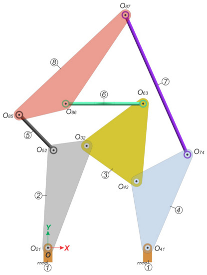
Figure 2. A, eight-bar “single flyer” undetermined planar linkage.

The first step in the process is to obtain the screws associated with the linkage’s kinematic pairs with respect to the origin of the coordinate system, O. To that end, the common direction of all revolute pairs, $\mathbf{u}$, is required, given by:

$$\mathbf{u}={\left[\begin{array}{ccc}0& 0& 1\end{array}\right]}^T$$

and by the position vectors of points located along the revolute axes, with respect to the origin, O. They are given in terms of an arbitrary unit of length, by:

$$\begin{array}{cccccc}\hfill {\mathbf{r}}_{21}& ={\left[\begin{array}{ccc}0& 0& 0\end{array}\right]}^T,\hfill & \hfill {\mathbf{r}}_{32}& ={\left[\begin{array}{ccc}70& 184& 0\end{array}\right]}^T,\hfill & \hfill {\mathbf{r}}_{43}& ={\left[\begin{array}{ccc}160& 120& 0\end{array}\right]}^T,\hfill \\ \hfill {\mathbf{r}}_{41}& ={\left[\begin{array}{ccc}180& 0& 0\end{array}\right]}^T,\hfill & \hfill {\mathbf{r}}_{52}& ={\left[\begin{array}{ccc}10& 176& 0\end{array}\right]}^T,\hfill & \hfill {\mathbf{r}}_{85}& ={\left[\begin{array}{ccc}-52& 240& 0\end{array}\right]}^T,\hfill \\ \hfill {\mathbf{r}}_{86}& ={\left[\begin{array}{ccc}32& 260& 0\end{array}\right]}^T,\hfill & \hfill {\mathbf{r}}_{63}& ={\left[\begin{array}{ccc}172& 260& 0\end{array}\right]}^T,\hfill & \hfill {\mathbf{r}}_{87}& ={\left[\begin{array}{ccc}140& 420& 0\end{array}\right]}^T,\hfill \\ \hfill {\mathbf{r}}_{74}& ={\left[\begin{array}{ccc}252& 168& 0\end{array}\right]}^T.\hfill \end{array}$$

From these data, the screws associated with the kinematic pairs, with respect to the origin of the coordinate system, O, are given by:

$$\begin{array}{cccccc}\hfill {}^2\${}_O^1& ={\left[\begin{array}{ccc}1;& 0& 0\end{array}\right]}^T,\hfill & \hfill {}^3\${}_O^2& ={\left[\begin{array}{ccc}1;& 184& -70\end{array}\right]}^T,\hfill & \hfill {}^4\${}_O^3& ={\left[\begin{array}{ccc}1;& 120& -160\end{array}\right]}^T,\hfill \\ \hfill {}^4\${}_O^1& ={\left[\begin{array}{ccc}1;& 0& -180\end{array}\right]}^T,\hfill & \hfill {}^5\${}_O^2& ={\left[\begin{array}{ccc}1;& 176& -10\end{array}\right]}^T,\hfill & \hfill {}^8\${}_O^5& ={\left[\begin{array}{ccc}1;& 240& 52\end{array}\right]}^T,\hfill \\ \hfill {}^8\${}_O^7& ={\left[\begin{array}{ccc}1;& 420& -140\end{array}\right]}^T,\hfill & \hfill {}^7\${}_O^4& ={\left[\begin{array}{ccc}1;& 168& -252\end{array}\right]}^T,\hfill & \hfill {}^8\${}_O^6& ={\left[\begin{array}{ccc}1;& 260& -32\end{array}\right]}^T,\hfill \\ \hfill {}^6\${}_O^3& ={\left[\begin{array}{ccc}1;& 260& -172\end{array}\right]}^T.\hfill \end{array}$$

It must be noted that, due to space considerations, only the non-zero terms are shown separated by a semicolon to indicate the different units.

3.1. Equations for the Location of Secondary IRCs

Regarding Figure 2, the primary IRCs are:

$$O_{21},O_{32},O_{43},O_{41},O_{52},O_{85},O_{87},O_{74},O_{86},O_{63}.$$

The upper triangular arrangement in Table 1 indicates the primary centers of the linkage with the number $-1$ and the secondary centers with the number $-2$.

Table 1. IRCs associated with the eight-bar planar linkage.

$O_{21}(-1)$	$O_{31}(-2)$	$O_{41}(-1)$	$O_{51}(-2)$	$O_{61}(-2)$	$O_{71}(-2)$	$O_{81}(-2)$
	$O_{32}(-1)$	$O_{42}(-2)$	$O_{52}(-1)$	$O_{62}(-2)$	$O_{72}(-2)$	$O_{82}(-2)$
		$O_{43}(-1)$	$O_{53}(-2)$	$O_{63}(-1)$	$O_{73}(-2)$	$O_{83}(-2)$
			$O_{54}(-2)$	$O_{64}(-2)$	$O_{74}(-1)$	$O_{84}(-2)$
				$O_{65}(-2)$	$O_{75}(-2)$	$O_{85}(-1)$
					$O_{76}(-2)$	$O_{86}(-1)$
						$O_{87}(-1)$

The linkage is denominated as partially undetermined because the direct application of the Aronhold–Kennedy theorem allows determining two secondary IRCs. Throughout this paper, whenever a sequence for determining an IRC is presented, the primary and secondary IRCs will be enclosed in boxes and circles, respectively. From Table 1, it follows that $O_{31}$ can be found using links 2 and 4.

The equations that determine the secondary center, and therefore, the screw characteristics, are:

$$\begin{array}{c}\hfill Ki({\$}_{a,Ki,Kl}^2,{}^3{\$}^1)=0Kl({\$}_{a,Ki,Kl}^2,{}^3{\$}^1)=0\end{array}$$

(25)

and

$$\begin{array}{c}\hfill Ki({\$}_{a,Ki,Kl}^4,{}^3{\$}^1)=0Kl({\$}_{a,Ki,Kl}^4,{}^3{\$}^1)=0\end{array}$$

(26)

where $\left\{{\$}_{a1,Ki,Kl}^2\right\}$ is a basis for the orthogonal annihilator of the subspace $[{}^2{\$}^1,{}^3{\$}^2]$, and $\left\{{\$}_{a1,Ki,Kl}^4\right\}$ is a basis for the orthogonal annihilator of the subspace $[{}^4{\$}^3,{}^4{\$}^1]$, regarding the Killing and Klein forms.

From Equations (25) and (26), and applying the Aronhold–Kennedy theorem with the Klein form, the equations necessary to determine the location of the secondary center $O_{31}$ are given by:

$$\begin{array}{ccc}\hfill Eq{31}_2& =& \left[0,180-\frac{1}{6}{y}_{31}-x_{31},0,0\right]\hfill \end{array}$$

(27)

$$\begin{array}{ccc}\hfill Eq{31}_4& =& \left[0,\frac{35}{92}{y}_{31}-x_{31},0,0\right].\hfill \end{array}$$

(28)

The vector expression $Eqi{j}_k$ indicates that it was obtained while finding the center $ij$ and using link k as a third link. The expression is implicitly equated to the vector $\mathbf{0}$ to form a vector equation; however, only the second component is different from zero. Hence, only one scalar equation is obtained. From Equations (27) and (28), one obtains:

$$\begin{array}{ccc}\hfill 0& =& 180-\frac{1}{6}{y}_{31}-x_{31}\hfill \end{array}$$

(29)

$$\begin{array}{ccc}\hfill 0& =& \frac{35}{92}{y}_{31}-x_{31}\hfill \end{array}$$

(30)

Equations (29) and (30) form a linear system of two equations in two unknowns, the coordinates $x_{31}$ and $y_{31}$ associated with the secondary center $O_{31}$. Solving the linear system, the position vector ${\mathbf{r}}_{31}$ and the infinitesimal screw associated with the secondary center $O_{31}$ are given by:

$${\mathbf{r}}_{31}={\left[\begin{array}{ccc}\frac{18900}{151}& \frac{49680}{151}& 0\end{array}\right]}^T,{}^3\${}_O^1={\left[\begin{array}{ccc}1;& \frac{49680}{151}& -\frac{18900}{151}\end{array}\right]}^T$$

Similarly, the secondary center $O_{42}$ can be found by using links 1 and 3, Table 1.

Following a similar process as in the secondary center $O_{31}$, the position vector and the screw associated with the secondary center $O_{42}$, are found as:

$${\mathbf{r}}_{42}={\left[\begin{array}{ccc}\frac{1315}{4}& 0& 0\end{array}\right]}^T,{}^4\${}_O^2={\left[\begin{array}{cccccc}0& 0& 1& 0& -\frac{1315}{4}& 0\end{array}\right]}^T.$$

There is no other additional secondary IRC that can be determined by the direct application of the Aronhold–Kennedy theorem. The IRCs $O_{31}$ and $O_{42}$ will also be marked with the number $-1$. Moreover, they will be regarded as primary centers for all purposes. Further, the upper triangular array of the IRCs, after this step, is given in Table 2.

Table 2. IRCs associated with the eight-bar planar linkage after determining $O_{31}$ and $O_{42}$.

$O_{21}(-1)$	$O_{31}(-1)$	$O_{41}(-1)$	$O_{51}(-2)$	$O_{61}(-2)$	$O_{71}(-2)$	$O_{81}(-2)$
	$O_{32}(-1)$	$O_{42}(-1)$	$O_{52}(-1)$	$O_{62}(-2)$	$O_{72}(-2)$	$O_{82}(-2)$
		$O_{43}(-1)$	$O_{53}(-2)$	$O_{63}(-1)$	$O_{73}(-2)$	$O_{83}(-2)$
			$O_{54}(-2)$	$O_{64}(-2)$	$O_{74}(-1)$	$O_{84}(-2)$
				$O_{65}(-2)$	$O_{75}(-2)$	$O_{85}(-1)$
					$O_{76}(-2)$	$O_{86}(-1)$
						$O_{87}(-1)$

The flow chart of the algorithm proposed for solving indeterminate linkages is presented in Figure 3. The computation of the undetermined IRCs starts at step 4. The first 3 steps are simple and they do not require additional explanation.

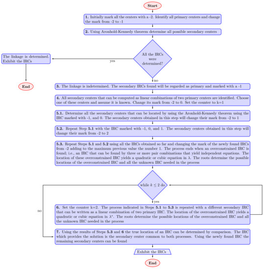
Figure 3. Flow diagram of the proposed algorithm.

Step 4.

Choose a secondary center, ${}^i{\$}^j$, whose location can be written as a linear combination of the position of two primary centers, namely, those marked with the number $-1$. Appendix A shows the procedure to accomplish this task; the secondary center can be written in terms of only one variable, denoted $\lambda$ or ${\lambda }^{\ast }$. From a theoretical point of view, any such center can be employed. However, it is convenient to choose secondary centers that yield a minimum number of equations. The marking of this secondary center will change from $-2$ to 0, and it will be assumed that its location is known. Set the counter $k=1$.

Step 5.1.

Determine all the secondary centers that can be located by the Aronhold–Kennedy theorem using the centers marked with $-1$ and 0, namely, the center chosen in step 1. The secondary centers obtained in this step will change their mark from $-2$ to 1.

Step 5.2.

Repeat Step 5.1, but now, it is necessary to locate all the secondary centers that can be determined, by using the Aronhold–Kennedy theorem, on the IRCs marked with the numbers $-1$, 0, and 1. The IRCs obtained in this step will change their mark from $-2$ to 2.

Step 5.3.

Repeat Step 5.2 using all the secondary centers obtained so far and changing the mark of the newly found IRCs, adding to the maximum previous value the number 1. The process finishes when an overconstrained center is found, namely, a rotation center that can be determined by using more than two pairs of already-known IRCs that yield independent equations. Simplifying the resulting system of equations yields a quadratic or cubic equation in $\lambda$. The roots of the equation determine the possible locations of the secondary center.

Step 6.

Set the counter $k=2$. Steps 5.1 to 5.3 must be repeated with a new secondary center that can be expressed as a linear combination of two primary centers. The process eventually yields an overconstrained secondary center, whose location can be obtained through a system of equations that yields a quadratic or cubic equation in ${\lambda }^{\ast }$. The roots of the equation determine the possible locations of the secondary center.

Step 7.

The correct location of the secondary center, obtained through the values of $\lambda$ and ${\lambda }^{\ast }$, is determined by choosing the location of a secondary center common to the two processes outlined in the two previous paragraphs. In the process, the location of many other secondary IRCs, usually all, are also found.

The proposed algorithm is used in the rest of the paper.

3.2. Determination and Solution of the System of Equations

The objective of this analysis is to determine the position vectors, in the plane $z=0$, of a point along the rotation axes of the relative movements associated with the secondary centers shown in Table 2. The secondary centers that can be written as a linear combination of two primary centers are $O_{51}$, $O_{61}$, $O_{71}$, $O_{62}$, $O_{72}$, $O_{82}$, $O_{53}$, $O_{73}$, $O_{83}$, $O_{54}$, $O_{64}$, $O_{84}$, $O_{65}$, $O_{75}$, and $O_{76}$. Table 3 shows only the secondary centers used in the process.

Table 3. Secondary centers whose location can be written as a linear combination of the location of two primary centers.

$O_{62}\mathrm{i}\mathrm{s} \mathrm{f}\mathrm{o}\mathrm{u}\mathrm{n}\mathrm{d} \mathrm{o}\mathrm{n} \mathrm{t}\mathrm{h}\mathrm{e} \mathrm{l}\mathrm{i}\mathrm{n}\mathrm{e} \mathrm{d}\mathrm{e}\mathrm{t}\mathrm{e}\mathrm{r}\mathrm{m}\mathrm{i}\mathrm{n}\mathrm{e}\mathrm{d} \mathrm{b}\mathrm{y}{O}_{32}\mathrm{a}\mathrm{n}\mathrm{d}{O}_{63}$

$O_{72}\mathrm{i}\mathrm{s} \mathrm{f}\mathrm{o}\mathrm{u}\mathrm{n}\mathrm{d} \mathrm{o}\mathrm{n} \mathrm{t}\mathrm{h}\mathrm{e} \mathrm{l}\mathrm{i}\mathrm{n}\mathrm{e} \mathrm{d}\mathrm{e}\mathrm{t}\mathrm{e}\mathrm{r}\mathrm{m}\mathrm{i}\mathrm{n}\mathrm{e}\mathrm{d} \mathrm{b}\mathrm{y}{O}_{42}\mathrm{a}\mathrm{n}\mathrm{d}{O}_{74}$

3.2.1. Selection of a First Arbitrary Center and Determination of an Overconstrained Center

From Table 3, the secondary center $O_{62}$ is chosen. This center can be written as:

$$\begin{array}{ccc}\hfill {\mathbf{r}}_{62}& =& \lambda {\mathbf{r}}_{32}+(1-\lambda ){\mathbf{r}}_{63}\hfill \end{array}$$

(31)

The upper triangular arrangement of centers, after this point, is given by:

$$\begin{array}{cccccccc}& \hfill O_{21}(-1)& \hfill O_{31}(-1)& \hfill O_{41}(-1)& \hfill O_{51}(-2)& \hfill O_{61}(-2)& \hfill O_{71}(-2)& \hfill O_{81}(-2)\\ & & \hfill O_{32}(-1)& \hfill O_{42}(-1)& \hfill O_{52}(-1)& \hfill O_{62}\left(0\right)& \hfill O_{72}(-2)& \hfill O_{82}(-2)\\ & & & \hfill O_{43}(-1)& \hfill O_{53}(-2)& \hfill O_{63}(-1)& \hfill O_{73}(-2)& \hfill O_{83}(-2)\\ & & & & \hfill O_{54}(-2)& \hfill O_{64}(-2)& \hfill O_{74}(-1)& \hfill O_{84}(-2)\\ & & & & & \hfill O_{65}(-2)& \hfill O_{75}(-2)& \hfill O_{85}(-1)\\ & & & & & & \hfill O_{76}(-2)& \hfill O_{86}(-1)\\ & & & & & & & \hfill O_{87}(-1)\end{array}$$

From this selection, it is possible to find the secondary centers. (The text shows only the required centers. However, the subsequent upper triangular arrangements show all centers that can be found. This convention will be followed in the rest of the contribution.) $O_{82}$ and $O_{64}$ are indicated, from now on, in blue color and dashed lines.

After identifying the secondary centers $O_{82}$ and $O_{64}$ with the number 1, the upper triangular arrangement of the IRCs is given by:

$$\begin{array}{cccccccc}& \hfill O_{21}(-1)& \hfill O_{31}(-1)& \hfill O_{41}(-1)& \hfill O_{51}(-2)& \hfill O_{61}\left(1\right)& \hfill O_{71}(-2)& \hfill O_{81}(-2)\\ & & \hfill O_{32}(-1)& \hfill O_{42}(-1)& \hfill O_{52}(-1)& \hfill O_{62}\left(0\right)& \hfill O_{72}(-2)& \hfill O_{82}\left(1\right)\\ & & & \hfill O_{43}(-1)& \hfill O_{53}(-2)& \hfill O_{63}(-1)& \hfill O_{73}(-2)& \hfill O_{83}(-2)\\ & & & & \hfill O_{54}(-2)& \hfill O_{64}\left(1\right)& \hfill O_{74}(-1)& \hfill O_{84}(-2)\\ & & & & & \hfill O_{65}\left(1\right)& \hfill O_{75}(-2)& \hfill O_{85}(-1)\\ & & & & & & \hfill O_{76}(-2)& \hfill O_{86}(-1)\\ & & & & & & & \hfill O_{87}(-1)\end{array}$$

The next step is to employ all the centers found so far to find all additional secondary centers. Therefore,

After identifying the overconstrained secondary center, indicated from now on in red color and dotted lines, $O_{84}$, with the number 2, the final upper triangular arrangement of IRCs is given by:

$$\begin{array}{cccccccc}& \hfill O_{21}(-1)& \hfill O_{31}(-1)& \hfill O_{41}(-1)& \hfill O_{51}\left(2\right)& \hfill O_{61}\left(1\right)& \hfill O_{71}(-2)& \hfill O_{81}\left(2\right)\\ & & \hfill O_{32}(-1)& \hfill O_{42}(-1)& \hfill O_{52}(-1)& \hfill O_{62}\left(0\right)& \hfill O_{72}\left(2\right)& \hfill O_{82}\left(1\right)\\ & & & \hfill O_{43}(-1)& \hfill O_{53}\left(2\right)& \hfill O_{63}(-1)& \hfill O_{73}(-2)& \hfill O_{83}\left(2\right)\\ & & & & \hfill O_{54}\left(2\right)& \hfill O_{64}\left(1\right)& \hfill O_{74}(-1)& \hfill O_{84}\left(2\right)\\ & & & & & \hfill O_{65}\left(1\right)& \hfill O_{75}(-2)& \hfill O_{85}(-1)\\ & & & & & & \hfill O_{76}\left(2\right)& \hfill O_{86}(-1)\\ & & & & & & & \hfill O_{87}(-1)\end{array}$$

From Equation (31), the position vector associated with the chosen secondary center $O_{62}$ is given by:

$${\mathbf{r}}_{62}={\left[\begin{array}{ccc}172-102\lambda & 260-76\lambda & 0\end{array}\right]}^T$$

(32)

The position vectors associated with the secondary centers involved in this step are:

$${\mathbf{r}}_{82}=\left[\begin{array}{ccc}{x}_{82}& y_{82}& 0\end{array}\right],{\mathbf{r}}_{64}=\left[\begin{array}{ccc}{x}_{64}& y_{64}& 0\end{array}\right],{\mathbf{r}}_{84}=\left[\begin{array}{ccc}{x}_{84}& y_{84}& 0\end{array}\right].$$

(33)

The required equations are obtained applying systematically the Aronhold–Kennedy theorem together with the Klein form, Equations (34)–(40). These are vector equations; however, only one component is different from zero. Due to space considerations, only the non-zero component is indicated. (The two numbers of the equation indicate the IRC to be calculated, and the subscript indicates the third link required to apply the Aronhold–Kennedy theorem.).

$$\begin{array}{ccc}\hfill Eq{82}_5& =& \frac{361}{2}-\frac{31}{32}{y}_{82}-x_{82}\hfill \end{array}$$

(34)

$$\begin{array}{ccc}\hfill Eq{82}_6& =& \frac{38\lambda x_{82}-51\lambda y_{82}+12044\lambda +70y_{82}-18200}{\lambda }\hfill \end{array}$$

(35)

$$\begin{array}{ccc}\hfill Eq{64}_3& =& \frac{1048}{7}+\frac{3}{35}{y}_{64}-x_{64}\hfill \end{array}$$

(36)

$$\begin{array}{ccc}\hfill Eq{64}_2& =& \frac{304\lambda x_{64}-408\lambda y_{64}-99940\lambda -1040x_{64}-627y_{64}+341900}{19\lambda -65}\hfill \end{array}$$

(37)

$$\begin{array}{ccc}\hfill Eq{84}_7& =& \frac{980}{3}-\frac{4}{9}{y}_{84}-x_{84}\hfill \end{array}$$

(38)

$$\begin{array}{ccc}\hfill Eq{84}_2& =& \frac{4x_{82}{y}_{84}-4x_{84}{y}_{82}+1315y_{82}-1315y_{84}}{y_{82}}\hfill \end{array}$$

(39)

$$\begin{array}{ccc}\hfill Eq{84}_6& =& \frac{x_{64}{y}_{84}-x_{84}{y}_{64}+260(x_{84}-x_{64})+32(y_{64}-y_{84})}{y_{64}-260}\hfill \end{array}$$

(40)

From Equations (34)–(40), the final set of equations is:

$$\begin{array}{ccc}\hfill 0& =& \frac{361}{2}-\frac{31}{32}{y}_{82}-x_{82}\hfill \end{array}$$

(41)

$$\begin{array}{ccc}\hfill 0& =& \frac{38\lambda x_{82}-51\lambda y_{82}+12044\lambda +70y_{82}-18200}{\lambda }\hfill \end{array}$$

(42)

$$\begin{array}{ccc}\hfill 0& =& \frac{1048}{7}+\frac{3}{35}{y}_{64}-x_{64}\hfill \end{array}$$

(43)

$$\begin{array}{ccc}\hfill 0& =& \frac{304\lambda x_{64}-408\lambda y_{64}-99940\lambda -1040x_{64}-627y_{64}+341900}{19\lambda -65}\hfill \end{array}$$

(44)

$$\begin{array}{ccc}\hfill 0& =& \frac{980}{3}-\frac{4}{9}{y}_{84}-x_{84}\hfill \end{array}$$

(45)

$$\begin{array}{ccc}\hfill 0& =& \frac{4x_{82}{y}_{84}-4x_{84}{y}_{82}+1315y_{82}-1315y_{84}}{4y_{82}}\hfill \end{array}$$

(46)

$$\begin{array}{ccc}\hfill 0& =& \frac{x_{64}{y}_{84}-x_{84}{y}_{64}+260(x_{84}-x_{64})+32(y_{64}-y_{84})}{y_{64}-260}\hfill \end{array}$$

(47)

The coordinates $y_{ij}$ of each linear equation are solved in terms of the corresponding coordinates $x_{ij}$. Thus, Equations (41), (43) and (45) yield the following coordinates: $y_{82}$, $y_{64}$, and $y_{82}$:

$$\begin{array}{ccc}\hfill y_{82}=\frac{5776-32x_{82}}{31},& y_{64}={\displaystyle \frac{35x_{64}-5240}{3}},& y_{84}=735-\frac{9}{4}{x}_{84}.\hfill \end{array}$$

(48)

Substituting the results of Equations (48) into Equations (42), (44), (46) and (47), it follows that:

$$\begin{array}{ccc}\hfill 0& =& \frac{-1405x_{82}\lambda -39394\lambda +1120x_{82}+79940}{\lambda }\hfill \end{array}$$

(49)

$$\begin{array}{ccc}\hfill 0& =& \frac{8x_{64}\lambda -1100\lambda +15x_{64}-2580}{19\lambda -65}\hfill \end{array}$$

(50)

$$\begin{array}{ccc}\hfill 0& =& \frac{604x_{82}{x}_{84}-196240x_{82}-274469x_{84}+89467340}{-361+2x_{82}}\hfill \end{array}$$

(51)

$$\begin{array}{ccc}\hfill 0& =& \frac{167x_{64}{x}_{84}-10180x_{64}-24944x_{84}+952960}{172-x_{64}}\hfill \end{array}$$

(52)

From Equation (52), $x_{84}$ is solved in terms of $x_{64}$ to obtain:

$$\begin{array}{ccc}\hfill x_{84}& =& \frac{20(509x_{64}-47648)}{167x_{64}-24944}\hfill \end{array}$$

(53)

The solution for $x_{84}$, from Equation (53), is substituted into Equation (51) to solve $x_{82}$ also in terms of $x_{64}$, so that:

$$\begin{array}{ccc}\hfill x_{82}& =& \frac{1}{2}\frac{37959223x_{64}-6156610471}{41599x_{64}-6749098}\hfill \end{array}$$

(54)

This result for $x_{82}$, from Equation (54), is substituted into Equation (49) to obtain a solution for $x_{64}$ in terms of $\lambda$. Therefore,

$$\begin{array}{ccc}\hfill x_{64}& =& \frac{296186633709\lambda -257240306960}{-1585973480+1826135817\lambda }\hfill \end{array}$$

(55)

Substituting the solution for $x_{64}$ into Equation (50), a quadratic equation in $\lambda$ is obtained:

$$0=\frac{40082630108{\lambda }^2-64664725545\lambda +25911886000}{\left(-1585973480+1826135817\lambda \right)\left(19\lambda -65\right)}$$

(56)

After clearing the denominator, the two possible solutions of Equation (56) are:

$${\lambda }_a=\frac{711865}{816796},{\lambda }_b=\frac{36400}{49073}.$$

(57)

The two roots of Equation (56) are substituted into (32), thus obtaining the possible position vectors of the secondary center $O_{62}$:

$$\begin{array}{ccc}\hfill {\mathbf{r}}_{62a}={\left[\begin{array}{ccc}\frac{33939341}{408398}& \frac{39566305}{204199}& 0\end{array}\right]}^T,& & {\mathbf{r}}_{62b}={\left[\begin{array}{ccc}\frac{4727756}{49073}& \frac{9992580}{49073}& 0\end{array}\right]}^T.\hfill \end{array}$$

(58)

Finally, position vectors in Equation (58) can be used to compute the two possible position vectors associated with the secondary center $O_{82}$:

$$\begin{array}{ccc}\hfill {\mathbf{r}}_{82a}={\left[\begin{array}{ccc}\frac{1286974}{2949}& -\frac{779024}{2949}& 0\end{array}\right]}^T& & {\mathbf{r}}_{82b}={\left[\begin{array}{ccc}-\frac{935697}{1436}& \frac{308360}{359}& 0\end{array}\right]}^T\hfill \end{array}$$

(59)

3.2.2. Selection of a Second Arbitrary Center and Determination of an Overconstrained Center

The procedure must be repeated for another secondary center. From Table 3, the secondary center $O_{72}$ is chosen. The location of this center can be written as:

$$\begin{array}{ccc}\hfill {\mathbf{r}}_{O72}& =& {\lambda }^{\ast }{\mathbf{r}}_{O42}+(1-{\lambda }^{\ast }){\mathbf{r}}_{O74}\hfill \end{array}$$

(60)

The upper triangular arrangement of centers becomes:

$$\begin{array}{cccccccc}& \hfill O_{21}(-1)& \hfill O_{31}(-1)& \hfill O_{41}(-1)& \hfill O_{51}(-2)& \hfill O_{61}(-2)& \hfill O_{71}(-2)& \hfill O_{81}(-2)\\ & & \hfill O_{32}(-1)& \hfill O_{42}(-1)& \hfill O_{52}(-1)& \hfill O_{62}(-2)& \hfill O_{72}\left(0\right)& \hfill O_{82}(-2)\\ & & & \hfill O_{43}(-1)& \hfill O_{53}(-2)& \hfill O_{63}(-1)& \hfill O_{73}(-2)& \hfill O_{83}(-2)\\ & & & & \hfill O_{54}(-2)& \hfill O_{64}(-2)& \hfill O_{74}(-1)& \hfill O_{84}(-2)\\ & & & & & \hfill O_{65}(-2)& \hfill O_{75}(-2)& \hfill O_{85}(-1)\\ & & & & & & \hfill O_{76}(-2)& \hfill O_{86}(-1)\\ & & & & & & & \hfill O_{87}(-1)\end{array}$$

Using the centers found up to this point, it is possible to find the following secondary centers: $O_{82}$, $O_{73}$.

After identifying the secondary centers $O_{82}$ and $O_{73}$ with the number 1, the upper diagonal arrangement becomes:

$$\begin{array}{cccccccc}& \hfill O_{21}(-1)& \hfill O_{31}(-1)& \hfill O_{41}(-1)& \hfill O_{51}(-2)& \hfill O_{61}(-2)& \hfill O_{71}\left(1\right)& \hfill O_{81}(-2)\\ & & \hfill O_{32}(-1)& \hfill O_{42}(-1)& \hfill O_{52}(-1)& \hfill O_{62}(-2)& \hfill O_{72}\left(0\right)& \hfill O_{82}\left(1\right)\\ & & & \hfill O_{43}(-1)& \hfill O_{53}(-2)& \hfill O_{63}(-1)& \hfill O_{73}\left(1\right)& \hfill O_{83}(-2)\\ & & & & \hfill O_{54}(-2)& \hfill O_{64}(-2)& \hfill O_{74}(-1)& \hfill O_{84}(-2)\\ & & & & & \hfill O_{65}(-2)& \hfill O_{75}\left(1\right)& \hfill O_{85}(-1)\\ & & & & & & \hfill O_{76}(-2)& \hfill O_{86}(-1)\\ & & & & & & & \hfill O_{87}(-1)\end{array}$$

The final step requires employing all the secondary centers found so far to find additional secondary centers, in particular, an overconstrained secondary center. Therefore,

After identifying the overconstrained secondary center $O_{83}$ with the number 2, the final upper triangular arrangement of centers becomes:

$$\begin{array}{cccccccc}& O_{21}(-1)& O_{31}(-1)& O_{41}(-1)& O_{51}\left(2\right)& O_{61}(-2)& O_{71}\left(1\right)& O_{81}\left(2\right)\\ & & O_{32}(-1)& O_{42}(-1)& O_{52}(-1)& O_{62}\left(2\right)& O_{72}\left(0\right)& O_{82}\left(1\right)\\ & & & O_{43}(-1)& O_{53}\left(2\right)& O_{63}(-1)& O_{73}\left(1\right)& O_{83}\left(2\right)\\ & & & & O_{54}\left(2\right)& O_{64}(-2)& O_{74}(-1)& O_{84}\left(2\right)\\ & & & & & O_{65}(-2)& O_{75}\left(1\right)& O_{85}(-1)\\ & & & & & & O_{76}\left(2\right)& O_{86}(-1)\\ & & & & & & & O_{87}(-1)\end{array}$$

Now, it is possible to generate the equations required for the location of the secondary centers involved in this process. From Equation (60), the position vector of the center $O_{72}$, the secondary center chosen, is given by:

$${\mathbf{r}}_{72}={\left[\begin{array}{ccc}252+\frac{307{\lambda }^{\ast }}{4}& 168-168{\lambda }^{\ast }& 0\end{array}\right]}^T$$

(61)

The position vectors of the centers $O_{82}$, $O_{73}$, and $O_{83}$ involved in this process are:

$$\begin{array}{ccc}\hfill {\mathbf{r}}_{82}={\left[\begin{array}{ccc}{x}_{82}& y_{82}& 0\end{array}\right]}^T,& {\mathbf{r}}_{73}={\left[\begin{array}{ccc}{x}_{73}& y_{73}& 0\end{array}\right]}^T,& {\mathbf{r}}_{83}={\left[\begin{array}{ccc}{x}_{83}& y_{83}& 0\end{array}\right]}^T.\hfill \end{array}$$

The equations are obtained by applying systematically the Aronhold–Kennedy theorem together with the Klein form. It should be noted that these expressions are equated to the vector $\mathbf{0}$, generating four scalar equations, only one of which is non-trivial. Due to space considerations, only the non-zero component is shown.

$$\begin{array}{ccc}\hfill Eq{82}_5& =& \frac{361}{2}-\frac{31}{32}{y}_{82}-x_{82},\hfill \end{array}$$

(62)

$$\begin{array}{ccc}\hfill Eq{82}_7& =& \frac{672{\lambda }^{\ast }{x}_{82}+307{\lambda }^{\ast }{y}_{82}-223020{\lambda }^{\ast }+1008x_{82}+448y_{82}-329280}{3+2{\lambda }^{\ast }},\hfill \end{array}$$

(63)

$$\begin{array}{ccc}\hfill Eq{73}_4& =& -70+\frac{23}{12}{y}_{73}-x_{73},\hfill \end{array}$$

(64)

$$\begin{array}{ccc}\hfill Eq{73}_2& =& \frac{672{\lambda }^{\ast }{x}_{73}+307{\lambda }^{\ast }{y}_{73}-103528{\lambda }^{\ast }+64x_{73}+728y_{73}-138432}{2+21{\lambda }^{\ast }},\hfill \end{array}$$

(65)

$$\begin{array}{ccc}\hfill Eq{83}_6& =& -260+y_{83},\hfill \end{array}$$

(66)

$$\begin{array}{ccc}\hfill Eq{83}_2& =& \frac{x_{82}{y}_{83}-x_{83}{y}_{82}-184x_{82}+184x_{83}+70y_{82}-70y_{83}}{y_{82}-184},\hfill \end{array}$$

(67)

$$\begin{array}{ccc}\hfill Eq{83}_7& =& \frac{x_{73}{y}_{83}-x_{83}{y}_{73}-420x_{73}+420x_{83}+140y_{73}-140y_{83}}{y_{73}-420},\hfill \end{array}$$

(68)

From Equations (62)–(68), a final set of equations is obtained:

$$\begin{array}{ccc}\hfill 0& =& \frac{361}{2}-\frac{31}{32}{y}_{82}-x_{82}\hfill \end{array}$$

(69)

$$\begin{array}{ccc}\hfill 0& =& \frac{672{\lambda }^{\ast }{x}_{82}+307{\lambda }^{\ast }{y}_{82}-223020{\lambda }^{\ast }+1008x_{82}+448y_{82}-329280}{3+2{\lambda }^{\ast }},\hfill \end{array}$$

(70)

$$\begin{array}{ccc}\hfill 0& =& -70+\frac{23}{12}{y}_{73}-x_{73}\hfill \end{array}$$

(71)

$$\begin{array}{ccc}\hfill 0& =& \frac{672{\lambda }^{\ast }{x}_{73}+307{\lambda }^{\ast }{y}_{73}-103528{\lambda }^{\ast }+64x_{73}+728y_{73}-138432}{2+21{\lambda }^{\ast }}\hfill \end{array}$$

(72)

$$\begin{array}{ccc}\hfill 0& =& -260+y83\hfill \end{array}$$

(73)

$$\begin{array}{ccc}\hfill 0& =& \frac{x_{82}{y}_{83}-x_{83}{y}_{82}-184x_{82}+184x_{83}+70y_{82}-70y_{83}}{y_{82}-184}\hfill \end{array}$$

(74)

$$\begin{array}{ccc}\hfill 0& =& \frac{x_{73}{y}_{83}-x_{83}{y}_{73}-420x_{73}+420x_{83}+140y_{73}-140y_{83}}{y_{73}-420}\hfill \end{array}$$

(75)

Systematically, the coordinates $y_{ij}$ are solved, from the linear equations, in terms of the coordinates $x_{ij}$. Hence, the coordinates $y_{82}$, $y_{73}$, and $y_{83}$, solved from Equations (69), (71) and (73), are given, respectively, by:

$$\begin{array}{ccc}\hfill y_{82}=\frac{5776-32x_{82}}{31},& y_{73}={\displaystyle \frac{840+12x_{73}}{23}},& y_{83}=260.\hfill \end{array}$$

(76)

Substituting the results of Equation (76) into Equations (70), (72), (74) and (75), it follows that:

$$\begin{array}{ccc}\hfill 0& =& \frac{1285097{\lambda }^{\ast }-2752{\lambda }^{\ast }{x}_{82}-4228x_{82}+1905008}{7812+5208{\lambda }^{\ast }}\hfill \end{array}$$

(77)

$$\begin{array}{ccc}\hfill 0& =& \frac{1664{\lambda }^{\ast }-15{\lambda }^{\ast }{x}_{73}-8x_{73}+2016}{2+21{\lambda }^{\ast }}\hfill \end{array}$$

(78)

$$\begin{array}{ccc}\hfill 0& =& \frac{8x_{82}{x}_{83}+29x_{82}-18x_{83}-39970}{-9+4x_{82}}\hfill \end{array}$$

(79)

$$\begin{array}{ccc}\hfill 0& =& \frac{3x_{73}{x}_{83}+500x_{73}-2205x_{83}+179900}{-735+x_{73}}\hfill \end{array}$$

(80)

From Equation (80), $x_{83}$ is solved in terms of $x_{73}$, to obtain:

$$\begin{array}{ccc}\hfill x_{83}& =& -\frac{500x_{73}+179900}{-2205+3x_{73}}\hfill \end{array}$$

(81)

The solution for $x_{83}$, obtained from Equation (81), is substituted into Equation (79) to solve $x_{73}$ in terms of $x_{82}$, thus obtaining:

$$\begin{array}{ccc}\hfill x_{73}& =& \left(-35\right)\frac{42947x_{82}-2610630}{3913x_{82}+110910}\hfill \end{array}$$

(82)

The result for $x_{73}$, obtained from Equation (82), is substituted into Equation (78) to solve $x_{82}$ in terms of ${\lambda }^{\ast }$:

$$\begin{array}{ccc}\hfill x_{82}& =& \frac{51566370{\lambda }^{\ast }+22060080}{1263409{\lambda }^{\ast }+865816}\hfill \end{array}$$

(83)

Finally, the solution for $x_{82}$, obtained from Equation (83), is substituted into Equation (77) to obtain a quadratic equation in ${\lambda }^{\ast }$:

$$\begin{array}{ccc}\hfill 0& =& \frac{47796531143{{\lambda }^{\ast }}^2+104539672384{\lambda }^{\ast }+50197302848}{\left(106126356{\lambda }^{\ast }+72728544\right)\left(3+2{\lambda }^{\ast }\right)}\hfill \\ \hfill \end{array}$$

(84)

After clearing the denominator, the possible solutions of the quadratic Equation (84) are given by:

$${\lambda }_a^{\ast }=-\frac{1138984}{1599991},{\lambda }_b^{\ast }=-\frac{44072}{29873}.$$

(85)

The two roots of Equation (85) are substituted into Equation (61) to obtain the two possible locations of the secondary center $O_{72}$:

$${\mathbf{r}}_{72a}={\left[\begin{array}{ccc}\frac{315780710}{1599991}& \frac{460147800}{1599991}& 0\end{array}\right]}^T,{\mathbf{r}}_{72b}={\left[\begin{array}{ccc}\frac{4145470}{29873}& \frac{12422760}{29873}& 0\end{array}\right]}^T.$$

(86)

Finally, from the position vectors ${\mathbf{r}}_{72a},{\mathbf{r}}_{72b}$, the two possible position vectors of the secondary center $O_{82}$ are given by:

$${\mathbf{r}}_{82a}={\left[\begin{array}{ccc}\frac{1286974}{2949}& -\frac{779024}{2949}& 0\end{array}\right]}^T,{\mathbf{r}}_{82b}={\left[\begin{array}{ccc}\frac{129290}{2389}& \frac{311664}{2389}& 0\end{array}\right]}^T.$$

(87)

Summarizing, in the first process, the secondary IRC $O_{62}$ is assumed to be known, and the overconstrained rotation center is $O_{84}$. In the second process, the secondary IRC $O_{72}$ is assumed to be known, and the overconstrained rotation center is $O_{83}$. The subgraphs of the secondary rotation centers needed to accomplish this task is shown in Figure 4.

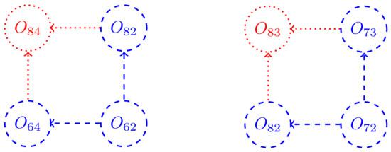
Figure 4. The subgraph of secondary rotation centers required to solve the “single-flyer” indeterminate planar linkage.

Comparing the results obtained in both processes for the position vector associated with IRC $O_{82}$, the only coincident result is given by:

$$\begin{array}{ccc}\hfill {\mathbf{r}}_{82a}& =& {\left[\begin{array}{ccc}\frac{1286974}{2949}& -\frac{779024}{2949}& 0\end{array}\right]}^T\hfill \end{array}$$

Therefore, the infinitesimal screw associated with the secondary center $O_{82}$ is given by:

$$\begin{array}{ccc}\hfill {}^8\${}_O^2& =& {\left[\begin{array}{ccc}1;& -\frac{779024}{2949}& -\frac{1286974}{2949}\end{array}\right]}^T\hfill \end{array}$$

(88)

Hence, the position vector associated with the secondary center $O_{62}$ is given by:

$$\begin{array}{ccc}\hfill {\mathbf{r}}_{62}& =& {\left[\begin{array}{ccc}\frac{33939341}{408398}& \frac{39566305}{204199}& 0\end{array}\right]}^T\hfill \end{array}$$

Furthermore, the infinitesimal screw associated with the secondary center $O_{62}$ is given by:

$$\begin{array}{ccc}\hfill {}^6\${}_O^2& =& {\left[\begin{array}{ccc}1;& \frac{39566305}{204199}& -\frac{33939341}{408398}\end{array}\right]}^T\hfill \end{array}$$

(89)

Finally from the result of Equation (89), together with the primary centers, applying the Aronhold–Kennedy theorem and using the Klein form, it is possible to find the remaining secondary centers following the procedure illustrated for the determination of the centers $O_{31}$ and $O_{42}$, Equations (25) and (26). Therefore, the position vectors corresponding to the remaining secondary centers are given by:

$$\begin{array}{cccc}\hfill {\mathbf{r}}_{72}& ={\left[\begin{array}{ccc}\frac{315780710}{1599991}& \frac{460147800}{1599991}& 0\end{array}\right]}^T,\hfill & \hfill {\mathbf{r}}_{64}& ={\left[\begin{array}{ccc}\frac{144519259}{897343}& \frac{118698915}{897343}& 0\end{array}\right]}^T,\hfill \\ \hfill {\mathbf{r}}_{84}& ={\left[\begin{array}{ccc}\frac{72796180}{206947}& -\frac{11685360}{206947}& 0\end{array}\right]}^T,\hfill & \hfill {\mathbf{r}}_{73}& ={\left[\begin{array}{ccc}-\frac{41572265}{133901}& -\frac{16799580}{133901}& 0\end{array}\right]}^T,\hfill \\ \hfill {\mathbf{r}}_{83}& ={\left[\begin{array}{ccc}\frac{68378}{8695}& 260& 0\end{array}\right]}^T,\hfill & \hfill {\mathbf{r}}_{76}& ={\left[\begin{array}{ccc}-\frac{112144664}{850397}& \frac{14647860}{850397}& 0\end{array}\right]}^T,\hfill \\ \hfill {\mathbf{r}}_{71}& ={\left[\begin{array}{ccc}\frac{5684052780}{11857451}& \frac{8282660400}{11857451}& 0\end{array}\right]}^T,\hfill & \hfill {\mathbf{r}}_{81}& ={\left[\begin{array}{ccc}-\frac{347482980}{1624111}& \frac{210336480}{1624111}& 0\end{array}\right]}^T,\hfill \\ \hfill {\mathbf{r}}_{75}& ={\left[\begin{array}{ccc}-\frac{9105880}{26227}& -\frac{3854865}{104908}& 0\end{array}\right]}^T,\hfill & \hfill {\mathbf{r}}_{51}& ={\left[\begin{array}{ccc}\frac{62723700}{3852029}& \frac{1103937120}{3852029}& 0\end{array}\right]}^T\hfill \\ \hfill {\mathbf{r}}_{53}& ={\left[\begin{array}{ccc}-\frac{99285}{241}& \frac{86570}{723}& 0\end{array}\right]}^T,\hfill & \hfill {\mathbf{r}}_{54}& ={\left[\begin{array}{ccc}\frac{56976220}{511177}& \frac{61329840}{511177}& 0\end{array}\right]}^T,\hfill \\ \hfill {\mathbf{r}}_{61}& ={\left[\begin{array}{ccc}\frac{3665448828}{27164597}& \frac{8546321880}{27164597}& 0\end{array}\right]}^T,\hfill & \hfill {\mathbf{r}}_{64}& ={\left[\begin{array}{ccc}\frac{144519259}{897343}& \frac{118698915}{897343}& 0\end{array}\right]}^T.\hfill \end{array}$$

The determination of the remaining infinitesimal screw representing the secondary IRCs is straightforward and, due to space considerations, is not presented here.

The location of the secondary IRCs, obtained from the position vectors, is shown in Figure 5. Therein, one can observe that the three centers associated with three relative movements, namely, ${}^i{\$}^k$, ${}^i{\$}^j$, and ${}^j{\$}^k$, between three arbitrary links lie on a straight line, according to the Aronhold–Kennedy theorem.

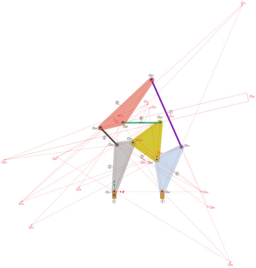
Figure 5. All rotation centers of a “single flyer” planar eight-bar linkage.

4. Second Case Study: Eight-Bar “Double-Butterfly” Planar Linkage

Consider the linkage shown in Figure 6, which is known as a “double-butterfly” eight-bar undetermined planar linkage. The linkage was proposed by Klein [4], who determined the secondary centers by using a trial-and-error method. Foster and Pennock [12] determined the secondary centers using a graphical method. Di Gregorio [13] determined the secondary centers by developing an algebraic method that combines the closure equations and the location of the secondary centers. This linkage has eight links, four of them ternary, and the remaining four binary, and it has ten revolutes. The linkage is trivial, and its mobility is 1.

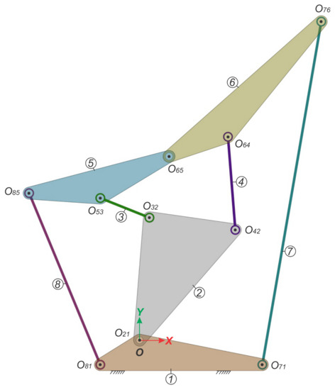
Figure 6. Eight-bar “double-butterfly” undetermined planar linkage.

The first step in the process is to obtain the screws associated with the linkage’s kinematic pairs about the origin of the coordinate system, O. To that end, the common direction of all revolute pairs, $\mathbf{u}$, is required, given by:

$$\mathbf{u}={\left[\begin{array}{ccc}0& 0& 1\end{array}\right]}^T$$

and the position vectors of points located along the revolute axes, about the origin, O. They are given in terms of an arbitrary unit of length, by:

$$\begin{array}{cccccc}\hfill {\mathbf{r}}_{21}& ={\left[\begin{array}{ccc}0& 0& 0\end{array}\right]}^T,\hfill & \hfill {\mathbf{r}}_{81}& ={\left[\begin{array}{ccc}-80& -50& 0\end{array}\right]}^T,\hfill & \hfill {\mathbf{r}}_{71}& ={\left[\begin{array}{ccc}250& -50& 0\end{array}\right]}^T,\hfill \\ \hfill {\mathbf{r}}_{32}& ={\left[\begin{array}{ccc}20& 250& 0\end{array}\right]}^T,\hfill & \hfill {\mathbf{r}}_{53}& ={\left[\begin{array}{ccc}-80& 290& 0\end{array}\right]}^T,\hfill & \hfill {\mathbf{r}}_{85}& ={\left[\begin{array}{ccc}-225& 300& 0\end{array}\right]}^T,\hfill \\ \hfill {\mathbf{r}}_{65}& ={\left[\begin{array}{ccc}60& 375& 0\end{array}\right]}^T,\hfill & \hfill {\mathbf{r}}_{42}& ={\left[\begin{array}{ccc}195& 225& 0\end{array}\right]}^T,\hfill & \hfill {\mathbf{r}}_{64}& ={\left[\begin{array}{ccc}180& 415& 0\end{array}\right]}^T,\hfill \\ \hfill {\mathbf{r}}_{76}& ={\left[\begin{array}{ccc}370& 650& 0\end{array}\right]}^T.\hfill \end{array}$$

From this data, the screws associated with the kinematic pairs, about the origin of the coordinate system, O, are given by:

$$\begin{array}{cccccc}\hfill {}^2\${}_O^1& ={\left[\begin{array}{ccc}1;& 0& 0\end{array}\right]}^T,\hfill & \hfill {}^3\${}_O^2& ={\left[\begin{array}{ccc}1;& 250& -20\end{array}\right]}^T,\hfill & \hfill {}^5\${}_O^3& ={\left[\begin{array}{ccc}1;& 290& 80\end{array}\right]}^T,\hfill \\ \hfill {}^8\${}_O^5& ={\left[\begin{array}{ccc}1;& 300& 225\end{array}\right]}^T,\hfill & \hfill {}^8\${}_O^1& ={\left[\begin{array}{ccc}1;& -50& 80\end{array}\right]}^T,\hfill & \hfill {}^4\${}_O^2& ={\left[\begin{array}{ccc}1;& 225& -195\end{array}\right]}^T,\hfill \\ \hfill {}^6\${}_O^4& ={\left[\begin{array}{ccc}1;& 415& -180\end{array}\right]}^T,\hfill & \hfill {}^6\${}_O^5& ={\left[\begin{array}{ccc}1;& 375& -60\end{array}\right]}^T,\hfill & \hfill {}^7\${}_O^6& ={\left[\begin{array}{ccc}1;& 650& -370\end{array}\right]}^T,\hfill \\ \hfill {}^7\${}_O^1& ={\left[\begin{array}{ccc}1;& -50& -250\end{array}\right]}^T.\hfill \end{array}$$

4.1. Determination of the Secondary Rotation Axes

From the enumeration of the links shown in Figure 6, the primary IRCs, namely, those that can be determined by inspection of the linkage, are:

$$O_{21},O_{32},O_{53},O_{85},O_{81},O_{42},O_{64},O_{65},O_{76},O_{71}$$

The upper diagonal arrangement of IRCs, where the primary centers are marked with the number $-1$, and the secondary centers are marked with the number $-2$, are shown in Table 4.

Table 4. Instantaneous rotation axes associated with the planar eight-bar linkage.

$O_{21}(-1)$	$O_{31}(-2)$	$O_{41}(-2)$	$O_{51}(-2)$	$O_{61}(-2)$	$O_{71}(-1)$	$O_{81}(-1)$
	$O_{32}(-1)$	$O_{42}(-1)$	$O_{52}(-2)$	$O_{62}(-2)$	$O_{72}(-2)$	$O_{82}(-2)$
		$O_{43}(-2)$	$O_{53}(-1)$	$O_{63}(-2)$	$O_{73}(-2)$	$O_{83}(-2)$
			$O_{54}(-2)$	$O_{64}(-1)$	$O_{74}(-2)$	$O_{84}(-2)$
				$O_{65}(-1)$	$O_{75}(-2)$	$O_{85}(-1)$
					$O_{76}(-1)$	$O_{86}(-2)$
						$O_{87}(-2)$

This linkage is completely undetermined since no secondary center can be found by the direct application of the Aronhold–Kennedy theorem. The search for these secondary IRCs will require two steps. In the first step, an arbitrary secondary center is chosen and the location of an overconstrained secondary center is determined up to the two possible roots of a quadratic equation. In the second step, another arbitrary secondary center is chosen and the location of the same overconstrained secondary center is determined up to the two possible roots of a quadratic equation. The comparison between the solutions of the two quadratic roots yields the correct solution and, from the intermediate results, the location of many other secondary centers will be accomplished. Therefore, Table 5 shows the secondary centers, which can be written as a linear combination of two primary centers employing a single variable $\lambda$, and which are used in this example.

Table 5. Secondary centers that can be written as a linear combination of two primary centers.

$O_{51}\mathrm{i}\mathrm{s} \mathrm{f}\mathrm{o}\mathrm{u}\mathrm{n}\mathrm{d} \mathrm{a}\mathrm{l}\mathrm{o}\mathrm{n}\mathrm{g} \mathrm{t}\mathrm{h}\mathrm{e} \mathrm{l}\mathrm{i}\mathrm{n}\mathrm{e} \mathrm{d}\mathrm{e}\mathrm{t}\mathrm{e}\mathrm{r}\mathrm{m}\mathrm{i}\mathrm{n}\mathrm{e}\mathrm{d} \mathrm{b}\mathrm{y}{O}_{81}{O}_{85}$

$O_{74}\mathrm{i}\mathrm{s} \mathrm{f}\mathrm{o}\mathrm{u}\mathrm{n}\mathrm{d} \mathrm{a}\mathrm{l}\mathrm{o}\mathrm{n}\mathrm{g} \mathrm{t}\mathrm{h}\mathrm{e} \mathrm{l}\mathrm{i}\mathrm{n}\mathrm{e} \mathrm{d}\mathrm{e}\mathrm{t}\mathrm{e}\mathrm{r}\mathrm{m}\mathrm{i}\mathrm{n}\mathrm{e}\mathrm{d} \mathrm{b}\mathrm{y}{O}_{76}{O}_{64}$

4.1.1. Selection of a First Arbitrary Center and Determination of an Overconstrained Center

From Table 5, the secondary center $O_{51}$ is chosen. This center can be written as:

$$\begin{array}{ccc}\hfill {\mathbf{r}}_{51}& =& \lambda {\mathbf{r}}_{81}+(1-\lambda ){\mathbf{r}}_{85}\hfill \end{array}$$

(90)

Thus, the upper triangular arrangement of IRC becomes:

$$\begin{array}{cccccccc}& \hfill O_{21}(-1)& \hfill O_{31}(-2)& \hfill O_{41}(-2)& \hfill O_{51}\left(0\right)& \hfill O_{61}(-2)& \hfill O_{71}(-1)& \hfill O_{81}(-1)\\ & & \hfill O_{32}(-1)& \hfill O_{42}(-1)& \hfill O_{52}(-2)& \hfill O_{62}(-2)& \hfill O_{72}(-2)& \hfill O_{82}(-2)\\ & & & \hfill O_{43}(-2)& \hfill O_{53}(-1)& \hfill O_{63}(-2)& \hfill O_{73}(-2)& \hfill O_{83}(-2)\\ & & & & \hfill O_{54}(-2)& \hfill O_{64}(-1)& \hfill O_{74}(-2)& \hfill O_{84}(-2)\\ & & & & & \hfill O_{65}(-1)& \hfill O_{75}(-2)& \hfill O_{85}(-1)\\ & & & & & & \hfill O_{76}(-1)& \hfill O_{86}(-2)\\ & & & & & & & \hfill O_{87}(-2)\end{array}$$

Therefore, following the approach indicated in Section 3.1, the application of the Aronhold–Kennedy theorem renders the location of the IRCs $O_{61}$, $O_{52}$

After marking the secondary IRCs $O_{61}$ and $O_{52}$ with the number 1, the upper triangular arrangement of the IRCs becomes:

$$\begin{array}{cccccccc}& \hfill O_{21}(-1)& \hfill O_{31}\left(1\right)& \hfill O_{41}(-2)& \hfill O_{51}\left(0\right)& \hfill O_{61}\left(1\right)& \hfill O_{71}(-1)& \hfill O_{81}(-1)\\ & & \hfill O_{32}(-1)& \hfill O_{42}(-1)& \hfill O_{52}\left(1\right)& \hfill O_{62}(-2)& \hfill O_{72}(-2)& \hfill O_{82}(-2)\\ & & & \hfill O_{43}(-2)& \hfill O_{53}(-1)& \hfill O_{63}(-2)& \hfill O_{73}(-2)& \hfill O_{83}(-2)\\ & & & & \hfill O_{54}(-2)& \hfill O_{64}(-1)& \hfill O_{74}(-2)& \hfill O_{84}(-2)\\ & & & & & \hfill O_{65}(-1)& \hfill O_{75}\left(1\right)& \hfill O_{85}(-1)\\ & & & & & & \hfill O_{76}(-1)& \hfill O_{86}(-2)\\ & & & & & & & \hfill O_{87}(-2)\end{array}$$

In the next step, all the IRCs found so far will be employed to find additional centers. In this case, the overconstrained center $O_{62}$ is found.

After marking the overconstrained IRC $O_{62}$ with the number 2, the upper triangular arrangement of the IRC is given by:

$$\begin{array}{cccccccc}& \hfill O_{21}(-1)& \hfill O_{31}\left(1\right)& \hfill O_{41}\left(2\right)& \hfill O_{51}\left(0\right)& \hfill O_{61}\left(1\right)& \hfill O_{71}(-1)& \hfill O_{81}(-1)\\ & & \hfill O_{32}(-1)& \hfill O_{42}(-1)& \hfill O_{52}\left(1\right)& \hfill O_{62}\left(2\right)& \hfill O_{72}\left(2\right)& \hfill O_{82}\left(2\right)\\ & & & \hfill O_{43}(-2)& \hfill O_{53}(-1)& \hfill O_{63}\left(2\right)& \hfill O_{73}\left(2\right)& \hfill O_{83}\left(2\right)\\ & & & & \hfill O_{54}\left(2\right)& \hfill O_{64}(-1)& \hfill O_{74}(-2)& \hfill O_{84}(-2)\\ & & & & & \hfill O_{65}(-1)& \hfill O_{75}\left(1\right)& \hfill O_{85}(-1)\\ & & & & & & \hfill O_{76}(-1)& \hfill O_{86}\left(2\right)\\ & & & & & & & \hfill O_{87}\left(2\right)\end{array}$$

From Equation (90), the position vector associated with the secondary IRC $O_{51}$ is:

$${\mathbf{r}}_{51}={\left[\begin{array}{ccc}145\lambda -225& -350\lambda +300& 0\end{array}\right]}^T$$

(91)

Furthermore, the position vectors associated with the involved IRC are:

$${\mathbf{r}}_{61}={\left[\begin{array}{ccc}{x}_{61}& y_{61}& 0\end{array}\right]}^T,{\mathbf{r}}_{52}={\left[\begin{array}{ccc}{x}_{52}& y_{52}& 0\end{array}\right]}^T,{\mathbf{r}}_{62}={\left[\begin{array}{ccc}{x}_{62}& y_{62}& 0\end{array}\right]}^T.$$

The necessary equations to solve the problem are obtained by systematically applying the Aronhold–Kennedy theorem employing the Klein form, Equations (25) and (26). It should be noted that these expressions are equated to the vector $\mathbf{0}$, generating four scalar equations, of which only one is non-trivial. Due to space considerations, only the non-zero component is shown.

$$\begin{array}{ccc}\hfill Eq{61}_7& =& \frac{1810}{7}+\frac{6}{35}{y}_{61}-x_{61},\hfill \end{array}$$

(92)

$$\begin{array}{ccc}\hfill Eq{61}_5& =& \frac{70\lambda x_{61}+29\lambda y_{61}-15075\lambda +15x_{61}-57y_{61}+20475}{3+14\lambda }\hfill \end{array}$$

(93)

$$\begin{array}{ccc}\hfill Eq{52}_3& =& 645-\frac{5}{2}{y}_{52}-x_{52},\hfill \end{array}$$

(94)

$$\begin{array}{ccc}\hfill Eq{52}_1& =& \frac{70\lambda x_{52}+29\lambda y_{52}-60x_{52}-45y_{52}}{7\lambda -6},\hfill \end{array}$$

(95)

$$\begin{array}{ccc}\hfill Eq{62}_4& =& \frac{8085}{38}-\frac{3}{38}{y}_{62}-x_{62},\hfill \end{array}$$

(96)

$$\begin{array}{ccc}\hfill Eq{62}_1& =& \frac{x_{61}{y}_{62}-x_{62}{y}_{61}}{y_{61}},\hfill \end{array}$$

(97)

$$\begin{array}{ccc}\hfill Eq{62}_5& =& \frac{x_{52}{y}_{62}-x_{62}{y}_{52}-375x_{52}+375x_{62}+60y_{52}-60y_{62}}{y_{52}-375}\hfill \end{array}$$

(98)

From Equations (92)–(98), the final set of equations is formed:

$$\begin{array}{ccc}\hfill 0& =& \frac{1810}{7}+\frac{6}{35}{y}_{61}-x_{61}\hfill \end{array}$$

(99)

$$\begin{array}{ccc}\hfill 0& =& \frac{70\lambda x_{61}+29\lambda y_{61}-15075\lambda +15x_{61}-57y_{61}+20475}{3+14\lambda }\hfill \end{array}$$

(100)

$$\begin{array}{ccc}\hfill 0& =& 645-\frac{5}{2}{y}_{52}-x_{52}\hfill \end{array}$$

(101)

$$\begin{array}{ccc}\hfill 0& =& \frac{70\lambda x_{52}+29\lambda y_{52}-60x_{52}-45y_{52}}{7\lambda -6}\hfill \end{array}$$

(102)

$$\begin{array}{ccc}\hfill 0& =& \frac{8085}{38}-\frac{3}{38}{y}_{62}-x_{62}\hfill \end{array}$$

(103)

$$\begin{array}{ccc}\hfill 0& =& \frac{x_{61}{y}_{62}-x_{62}{y}_{61}}{y_{61}}\hfill \end{array}$$

(104)

$$\begin{array}{ccc}\hfill 0& =& \frac{x_{52}{y}_{62}-x_{62}{y}_{52}-375x_{52}+375x_{62}+60y_{52}-60y_{62}}{y_{52}-375}\hfill \end{array}$$

(105)

Systematically, the coordinates $y_{ij}$ from each linear equation are solved in terms of the coordinates $x_{ij}$. Therefore, the coordinates $y_{61}$, $y_{52}$, and $y_{62}$ from Equations (99), (101) and (103) are written as:

$$\begin{array}{ccc}\hfill y_{61}=-\frac{4525}{3}+\frac{35x_{61}}{6},& y_{52}=258-{\displaystyle \frac{2x_{52}}{5}},& y_{62}=2695-\frac{38x_{62}}{3}.\hfill \end{array}$$

(106)

Substituting the results of Equation (106) into Equations (100), (102), (104) and (105), it follows that:

$$\begin{array}{ccc}\hfill 0& =& \frac{287\lambda x_{61}-70580\lambda -381x_{61}+127740}{3+14\lambda }\hfill \end{array}$$

(107)

$$\begin{array}{ccc}\hfill 0& =& \frac{146\lambda x_{52}+18705\lambda -105x_{52}-29025}{7\lambda -6}\hfill \end{array}$$

(108)

$$\begin{array}{ccc}\hfill 0& =& \frac{111x_{61}{x}_{62}-16170x_{61}-9050x_{62}}{-1810+7x_{61}}\hfill \end{array}$$

(109)

$$\begin{array}{ccc}\hfill 0& =& \frac{184x_{52}{x}_{62}-34440x_{52}-13155x_{62}+2193300}{585+2x_{52}}\hfill \end{array}$$

(110)

From Equation (110), $x_{62}$ is solved in terms of $x_{52}$ to obtain:

$$\begin{array}{ccc}\hfill x_{62}& =& \frac{60(574x_{52}-36555)}{184x_{52}-13155}\hfill \end{array}$$

(111)

The result for $x_{62}$, obtained from Equation (111), is substituted into Equation (109) to solve $x_{52}$ in terms of $x_{61}$, so that:

$$\begin{array}{ccc}\hfill x_{52}& =& \frac{1024665x_{61}-661645500}{28252x_{61}-10389400}\hfill \end{array}$$

(112)

Similarly, the result for $x_{52}$ of Equation (112) is substituted into Equation (108) to solve $x_{61}$ in terms of $\lambda$, therefore:

$$\begin{array}{ccc}\hfill x_{61}& =& \frac{3620(214316\lambda -273315)}{-2473611+1808146\lambda }\hfill \end{array}$$

(113)

Finally, the result for $x_{61}$, from Equation (113), is substituted into Equation (107) to obtain a quadratic equation in $\lambda$, given by:

$$\begin{array}{ccc}\hfill 0& =& \frac{-60(264007001{\lambda }^2-483296570\lambda +169395681)}{\left(-2473611+1808146\lambda \right)\left(3+14\lambda \right)}\hfill \end{array}$$

After clearing the denominator, the two solutions of $\lambda$ are given by:

$${\lambda }_a=\frac{1861491}{3940403},{\lambda }_b=\frac{91}{67}.$$

(114)

These solutions are substituted into Equation (91) to obtain the two possible locations of the center $O_{51}$.

$${\mathbf{r}}_{51a}={\left[\begin{array}{ccc}-\frac{616674480}{3940403}& \frac{530599050}{3940403}& 0\end{array}\right]}^T,{\mathbf{r}}_{51b}={\left[\begin{array}{ccc}-\frac{1880}{67}& -\frac{11750}{67}& 0\end{array}\right]}^T$$

(115)

4.1.2. Selection of a Second Arbitrary Center and Determination of an Overconstrained Center

The process must be repeated with another secondary center. From Table 5, the center $O_{74}$ is chosen, and its position vector can be written as:

$$\begin{array}{ccc}\hfill {\mathbf{r}}_{74}& =& {\lambda }^{\ast }{\mathbf{r}}_{76}+(1-{\lambda }^{\ast }){\mathbf{r}}_{64}={\left[\begin{array}{ccc}180+190{\lambda }^{\ast }& 415+235{\lambda }^{\ast }& 0\end{array}\right]}^T\hfill \end{array}$$

(116)

The upper triangular array of IRCs, with the center $O_{74}$ marked with the number 0, is given by:

$$\begin{array}{cccccccc}& \hfill O_{21}(-1)& \hfill O_{31}(-2)& \hfill O_{41}(-2)& \hfill O_{51}(-2)& \hfill O_{61}(-2)& \hfill O_{71}(-1)& \hfill O_{81}(-1)\\ & & \hfill O_{32}(-1)& \hfill O_{42}(-1)& \hfill O_{52}(-2)& \hfill O_{62}(-2)& \hfill O_{72}(-2)& \hfill O_{82}(-2)\\ & & & \hfill O_{43}(-2)& \hfill O_{53}(-1)& \hfill O_{63}(-2)& \hfill O_{73}(-2)& \hfill O_{83}(-2)\\ & & & & \hfill O_{54}(-2)& \hfill O_{64}(-1)& \hfill O_{74}\left(0\right)& \hfill O_{84}(-2)\\ & & & & & \hfill O_{65}(-1)& \hfill O_{75}(-2)& \hfill O_{85}(-1)\\ & & & & & & \hfill O_{76}(-1)& \hfill O_{86}(-2)\\ & & & & & & & \hfill O_{87}(-2)\end{array}$$

Using this secondary center $O_{74}$, the secondary centers $O_{41}$ and $O_{72}$ can be found:

After identifying the secondary centers $O_{41}$ and $O_{72}$ with the number 1, the upper triangular arrangement of centers becomes:

$$\begin{array}{cccccccc}& \hfill O_{21}(-1)& \hfill O_{31}(-2)& \hfill O_{41}\left(1\right)& \hfill O_{51}(-2)& \hfill O_{61}\left(1\right)& \hfill O_{71}(-1)& \hfill O_{81}(-1)\\ & & \hfill O_{32}(-1)& \hfill O_{42}(-1)& \hfill O_{52}(-2)& \hfill O_{62}(-2)& \hfill O_{72}\left(1\right)& \hfill O_{82}(-2)\\ & & & \hfill O_{43}(-2)& \hfill O_{53}(-1)& \hfill O_{63}(-2)& \hfill O_{73}(-2)& \hfill O_{83}(-2)\\ & & & & \hfill O_{54}(-2)& \hfill O_{64}(-1)& \hfill O_{74}\left(0\right)& \hfill O_{84}(-2)\\ & & & & & \hfill O_{65}(-1)& \hfill O_{75}(-2)& \hfill O_{85}(-1)\\ & & & & & & \hfill O_{76}(-1)& \hfill O_{86}(-2)\\ & & & & & & & \hfill O_{87}\left(1\right)\end{array}$$

The next step employs all the centers found so far to find additional centers. The relevant ones are:

After this step, the upper triangular arrangement of centers becomes:

$$\begin{array}{cccccccc}& \hfill O_{21}(-1)& \hfill O_{31}(-2)& \hfill O_{41}\left(1\right)& \hfill O_{51}(-2)& \hfill O_{61}\left(2\right)& \hfill O_{71}(-1)& \hfill O_{81}(-1)\\ & & \hfill O_{32}(-1)& \hfill O_{42}(-1)& \hfill O_{52}(-2)& \hfill O_{62}\left(2\right)& \hfill O_{72}\left(1\right)& \hfill O_{82}(-2)\\ & & & \hfill O_{43}(-2)& \hfill O_{53}(-1)& \hfill O_{63}(-2)& \hfill O_{73}(-2)& \hfill O_{83}(-2)\\ & & & & \hfill O_{54}(-2)& \hfill O_{64}(-1)& \hfill O_{74}\left(0\right)& \hfill O_{84}(-2)\\ & & & & & \hfill O_{65}(-1)& \hfill O_{75}(-2)& \hfill O_{85}(-1)\\ & & & & & & \hfill O_{76}(-1)& \hfill O_{86}(-2)\\ & & & & & & & \hfill O_{87}(-2)\end{array}$$

The following step employs all the IRCs marked with the numbers $-1,0,1$, and 2 to find additional IRCs; the relevant ones are:

Marking the newly found IRCs with the number 3, the upper triangular arrangement of centers becomes:

$$\begin{array}{cccccccc}& \hfill O_{21}(-1)& \hfill O_{31}(-2)& \hfill O_{41}\left(1\right)& \hfill O_{51}\left(3\right)& \hfill O_{61}\left(2\right)& \hfill O_{71}(-1)& \hfill O_{81}(-1)\\ & & \hfill O_{32}(-1)& \hfill O_{42}(-1)& \hfill O_{52}\left(3\right)& \hfill O_{62}\left(2\right)& \hfill O_{72}\left(1\right)& \hfill O_{82}(-2)\\ & & & \hfill O_{43}(-2)& \hfill O_{53}(-1)& \hfill O_{63}\left(3\right)& \hfill O_{73}(-2)& \hfill O_{83}(-2)\\ & & & & \hfill O_{54}(-2)& \hfill O_{64}(-1)& \hfill O_{74}\left(0\right)& \hfill O_{84}(-2)\\ & & & & & \hfill O_{65}(-1)& \hfill O_{75}(-2)& \hfill O_{85}(-1)\\ & & & & & & \hfill O_{76}(-1)& \hfill O_{86}\left(3\right)\\ & & & & & & & \hfill O_{87}(-2)\end{array}$$

The final step is to find an overconstrained IRC. In this case, the IRC $O_{31}$ can be found using the following three IRC combinations:

The position vectors of the secondary centers found in this process are:

$$\begin{array}{cccc}\hfill & {\mathbf{r}}_{31}={\left[\begin{array}{ccc}{x}_{31}& y_{31}& 0\end{array}\right]}^T,\hfill & \hfill {\mathbf{r}}_{41}={\left[\begin{array}{ccc}{x}_{41}& y_{41}& 0\end{array}\right]}^T,& {\mathbf{r}}_{51}={\left[\begin{array}{ccc}{x}_{51}& y_{51}& 0\end{array}\right]}^T,\hfill \\ \hfill & {\mathbf{r}}_{61}={\left[\begin{array}{ccc}{x}_{61}& y_{61}& 0\end{array}\right]}^T,\hfill & \hfill {\mathbf{r}}_{62}={\left[\begin{array}{ccc}{x}_{62}& y_{62}& 0\end{array}\right]}^T,& {\mathbf{r}}_{63}={\left[\begin{array}{ccc}{x}_{63}& y_{63}& 0\end{array}\right]}^T.\hfill \\ \hfill & {\mathbf{r}}_{72}={\left[\begin{array}{ccc}{x}_{72}& y_{72}& 0\end{array}\right]}^T.\hfill \end{array}$$

The equations required to solve the problem are obtained applying the Aronhold–Kennedy theorem and using systematically the Klein form, Equations (25) and (26). It should be noted that these expressions are equated to the vector $\mathbf{0}$, generating four scalar equations, of which only one is non-trivial. Due to space considerations, only the non-zero component is shown.

$$\begin{array}{cc}\hfill & Eq{41}_2=225x_{41}-195y_{41}=0,\hfill \end{array}$$

(117)

$$\begin{array}{cc}\hfill & Eq{41}_7=235{\lambda }^{\ast }{x}_{41}-190{\lambda }^{\ast }{y}_{41}-68250{\lambda }^{\ast }+465x_{41}+70y_{41}-112750=0,\hfill \end{array}$$

(118)

$$\begin{array}{cc}\hfill & Eq{72}_1=-50x_{72}-250y_{72}\hfill \end{array}$$

(119)

$$\begin{array}{cc}\hfill & Eq{72}_4=235{\lambda }^{\ast }{x}_{72}-190{\lambda }^{\ast }{y}_{72}-3075{\lambda }^{\ast }+190x_{72}+15y_{72}-40425=0\hfill \end{array}$$

(120)

$$\begin{array}{cc}\hfill & Eq{61}_7=700x_{61}-120y_{61}-181000=0,\hfill \end{array}$$

(121)

$$\begin{array}{cc}\hfill & Eq{61}_4=x_{41}{y}_{61}-x_{61}{y}_{41}-415x_{41}+415x_{61}+180y_{41}-180y_{61}=0,\hfill \end{array}$$

(122)

$$\begin{array}{cc}\hfill & Eq{62}_4=190x_{62}+15y_{62}-40425=0,\hfill \end{array}$$

(123)

$$\begin{array}{cc}\hfill & Eq{62}_7=-x_{62}{y}_{72}+x_{72}{y}_{62}+650x_{62}-650x_{72}-370y_{62}+370y_{72}=0,\hfill \end{array}$$

(124)

$$\begin{array}{cc}\hfill & Eq{63}_2=-x_{62}{y}_{63}+x_{63}{y}_{62}+250x_{62}-250x_{63}-20y_{62}+20y_{63}=0,\hfill \end{array}$$

(125)

$$\begin{array}{cc}\hfill & Eq{63}_5=85x_{63}-140y_{63}+47400=0,\hfill \end{array}$$

(126)

$$\begin{array}{cc}\hfill & Eq{51}_6=-x_{51}{y}_{61}+x_{61}{y}_{51}+375x_{51}-375x_{61}-60y_{51}+60y_{61}=0,\hfill \end{array}$$

(127)

$$\begin{array}{cc}\hfill & Eq{51}_8=350x_{51}+145y_{51}+35250=0,\hfill \end{array}$$

(128)

$$\begin{array}{cc}\hfill & Eq{31}_2=250x_{31}-20y_{31}=0,\hfill \end{array}$$

(129)

$$\begin{array}{cc}\hfill & Eq{31}_5=-x_{31}{y}_{51}+x_{51}{y}_{31}+290x_{31}-290x_{51}+80y_{31}-80y_{51}=0,\hfill \end{array}$$

(130)

$$\begin{array}{cc}\hfill & Eq{31}_6=-x_{31}{y}_{61}+x_{31}{y}_{63}+x_{61}{y}_{31}-x_{61}{y}_{63}-x_{63}{y}_{31}+x_{63}{y}_{61}=0.\hfill \end{array}$$

(131)

Equations (117)–(131) represent a system of 15 equations in 15 unknowns. The solution requires that the coordinates $y_{ij}$ are solved in terms of the coordinates $x_{ij}$ from the linear equations. Hence, the coordinates $y_{41}$, $y_{72}$, $y_{61}$, $y_{62}$, $y_{63}$, $y_{51}$, and $y_{31}$ are solved from Equations (117), (119), (121), (123), (126), (128) and (129), and one obtains:

$$\begin{array}{ccc}\hfill y_{41}=\frac{15}{13}{x}_{41},& y_{72}=-\frac{1}{5}{x}_{72},& y_{61}=\frac{35}{6}{x}_{61}-\frac{4525}{3}\hfill \end{array}$$

(132)

$$\begin{array}{ccc}\hfill y_{62}=-\frac{38}{3}{x}_{62}+2695,& y_{51}=-\frac{70}{29}{x}_{51}-\frac{7050}{29}& y_{63}=\frac{17}{28}{x}_{63}+\frac{2370}{7}\hfill \end{array}$$

(133)

$$\begin{array}{ccc}\hfill y_{31}=\frac{25}{2}{x}_{3}1& & \hfill \end{array}$$

(134)

Substituting the results of Equations (132)–(134) into the remaining non-linear equations, it follows that:

$$\begin{array}{ccc}\hfill 0& =& \frac{205}{13}{x}_{41}{\lambda }^{\ast }-68250{\lambda }^{\ast }+\frac{7095}{13}{x}_{41}-112750\hfill \end{array}$$

(135)

$$\begin{array}{ccc}\hfill 0& =& -\frac{1435}{174}{x}_{51}{x}_{61}+\frac{176450}{87}{x}_{51}-\frac{7775}{29}{x}_{61}-\frac{2201500}{29}\hfill \end{array}$$

(136)

$$\begin{array}{ccc}\hfill 0& =& \frac{365}{78}{x}_{61}{x}_{41}-\frac{66910}{39}{x}_{41}-635x_{61}+271500\hfill \end{array}$$

(137)

$$\begin{array}{ccc}\hfill 0& =& -\frac{187}{15}{x}_{62}{x}_{72}+1971x_{72}+\frac{16010}{3}{x}_{62}-997150\hfill \end{array}$$

(138)

$$\begin{array}{ccc}\hfill 0& =& -\frac{1115}{84}{x}_{62}{x}_{63}+\frac{3460}{21}{x}_{62}+\frac{17200}{7}{x}_{63}-\frac{329900}{7}\hfill \end{array}$$

(139)

$$\begin{array}{ccc}\hfill 0& =& 273{\lambda }^{\ast }{x}_{72}-3075{\lambda }^{\ast }+187x_{72}-40425\hfill \end{array}$$

(140)

$$\begin{array}{ccc}\hfill 0& =& \frac{865}{58}{x}_{31}{x}_{51}+\frac{44460}{29}{x}_{31}-\frac{2810}{29}{x}_{51}+\frac{564000}{29}\hfill \end{array}$$

(141)

$$\begin{array}{ccc}\hfill 0& =& \frac{20}{3}{x}_{31}{x}_{61}+\frac{38785}{21}{x}_{31}-\frac{333}{28}{x}_{31}{x}_{63}+\frac{439}{84}{x}_{61}{x}_{63}-\frac{2370}{7}{x}_{61}-\frac{4525}{3}{x}_{63}\hfill \end{array}$$

(142)

From Equation (135), $x_{41}$ is solved in terms of ${\lambda }^{\ast }$. The result given by

$$x_{41}=\frac{650(273{\lambda }^{\ast }+451)}{41{\lambda }^{\ast }+1419},$$

(143)

is substituted into Equation (137). Furthermore, solving the resulting equation for $x_{61}$, one obtains:

$$0=\frac{921{\lambda }^{\ast }{x}_{61}-335850{\lambda }^{\ast }+539x_{61}-134750}{41{\lambda }^{\ast }+1419}{x}_{61}=\frac{50(6717{\lambda }^{\ast }+2695)}{921{\lambda }^{\ast }+539}.$$

(144)

The result for $x_{61}$ is substituted into Equation (136), to obtain:

$$0=\frac{1046159{\lambda }^{\ast }{x}_{51}+185552610{\lambda }^{\ast }+21021x_{51}+89371590}{921{\lambda }^{\ast }+539}.$$

(145)

Solving Equation (145) for $x_{51}$, it follows that:

$$x_{51}=-\frac{30(6185087{\lambda }^{\ast }+2979053)}{1046159{\lambda }^{\ast }+21021}$$

(146)

The value of $x_{61}$, from Equation (143), is also substituted into Equation (137). The result is given by:

$$0=\frac{35382{\lambda }^{\ast }{x}_{62}-7437465{\lambda }^{\ast }-24973x_{62}+4201260}{381{\lambda }^{\ast }-94}.$$

(147)

The resulting equation, (147), is solved for $x_{62}$ in terms of ${\lambda }^{\ast }$; hence:

$$x_{62}=\frac{735(10119{\lambda }^{\ast }-5716)}{35382{\lambda }^{\ast }-24973}.$$

(148)

In the next step, $x_{72}$ is solved from Equation (140), and the result is given by:

$$x_{72}=\frac{75(41{\lambda }^{\ast }+539)}{273{\lambda }^{\ast }+187}.$$

(149)

The value of $x_{72}$ is substituted into Equation (138). Furthermore, solving the resulting equation for $x_{62}$, one obtains:

$$0=\frac{537{\lambda }^{\ast }{x}_{62}-100755{\lambda }^{\ast }+187x_{62}-40425}{273{\lambda }^{\ast }+187}{x}_{62}=\frac{15(6717{\lambda }^{\ast }+2695)}{537{\lambda }^{\ast }+187}.$$

(150)

Repeating the process by substituting the value of $x_{62}$ into (139), and then solving for $x_{63}$, it follows that:

$$0=\frac{6689{\lambda }^{\ast }{x}_{63}+3250784{\lambda }^{\ast }+28787x_{63}+803616}{537{\lambda }^{\ast }+187}{x}_{63}=-\frac{32(101587{\lambda }^{\ast }+25113)}{6689{\lambda }^{\ast }+28787}.$$

(151)

Before the final substitutions, the value of $x_{51}$ is substituted into (141) to obtain:

$$0=-\frac{77561551{\lambda }^{\ast }{x}_{31}-2555026460{\lambda }^{\ast }+86709469x_{31}-604574740}{1046159{\lambda }^{\ast }+21021}.$$

Then, solving for $x_{31}$ a solution in terms of ${\lambda }^{\ast }$ is given by:

$$x_{31}=-\frac{140(18250189{\lambda }^{\ast }+4318391)}{77561551{\lambda }^{\ast }+86709469}.$$

(152)

Similarly, the value of $x_{61}$ is substituted into Equation (131) to obtain:

$$0=\frac{c_1{{\lambda }^{\ast }}^2{x}_{31}-c_2{{\lambda }^{\ast }}^2+c_3{\lambda }^{\ast }{x}_{31}-c_4{\lambda }^{\ast }+c_5{x}_{31}-c_6}{(921{\lambda }^{\ast }+539)(6689{\lambda }^{\ast }+28787)},$$

(153)

where

$$\begin{array}{ccc}\hfill c_1=61961537269& c_2=1950521392700& c_3=155729090462\hfill \\ \hfill c_4=3519109121000& c_5=59668631869& c_6=1225931622300\hfill \end{array}$$

Substituting the value of $x_{31}$ obtained in Equation (152) into Equation (153), a final cubic equation in ${\lambda }^{\ast }$ is obtained:

$$0=\frac{d_1{{\lambda }^{\ast }}^3-d_2{{\lambda }^{\ast }}^2-D_3{\lambda }^{\ast }-d_4}{(77561551{\lambda }^{\ast }+86709469)(921{\lambda }^{\ast }+539)(6689{\lambda }^{\ast }+28787)}.$$

(154)

where

$$\begin{array}{ccc}\hfill d_1=175697568701976501& & d_2=168097719765363443\hfill \\ \hfill d_3=3840510841167663817& & d_4=1755643310039629241\hfill \end{array}$$

After clearing the denominator of (153), its solutions are given by:

$${\lambda }_a^{\ast }=\frac{815507}{151807},{\lambda }_b^{\ast }=-\frac{31449671}{7974909},{\lambda }_c^{\ast }=-\frac{68453}{145127}$$

(155)

The results for ${\lambda }^{\ast }$ are substituted into Equation (116) to obtain the three possible position vectors of the secondary center $O_{74}$:

$$\begin{array}{ccc}\hfill {\mathbf{r}}_{74a}=\left[\begin{array}{c}\frac{182271590}{151807}\\ \frac{254644050}{151807}\end{array}\right]& {\mathbf{r}}_{74b}=\left[\begin{array}{c}-\frac{4539953870}{7974909}\\ -\frac{4081085450}{7974909}\\ 0\end{array}\right]& {\mathbf{r}}_{74c}=\left[\begin{array}{c}\frac{13116790}{145127}\\ \frac{44141250}{145127}\\ 0\end{array}\right].\hfill \end{array}$$

(156)

From the results of Equation (156), it is possible to find the three possible locations of the secondary centers $O_{41}$ and $O_{61}$:

$$\begin{array}{ccc}\hfill {\mathbf{r}}_{41a}=\left[\begin{array}{c}\frac{6719245}{8837}\\ \frac{7752975}{8837}\\ 0\end{array}\right]& {\mathbf{r}}_{41b}=\left[\begin{array}{c}-\frac{115159785}{356071}\\ -\frac{132876675}{356071}\\ 0\end{array}\right]& {\mathbf{r}}_{41c}=\left[\begin{array}{c}\frac{664270}{4439}\\ \frac{9964050}{57707}\\ 0\end{array}\right],\hfill \end{array}$$

(157)

and

$$\begin{array}{ccc}\hfill {\mathbf{r}}_{61a}=\left[\begin{array}{c}\frac{155140}{439}\\ \frac{242825}{439}\\ 0\end{array}\right]& {\mathbf{r}}_{61b}=\left[\begin{array}{c}\frac{898461460}{2335859}\\ \frac{5153313575}{7007577}\\ 0\end{array}\right]& {\mathbf{r}}_{61c}=\left[\begin{array}{c}-\frac{905}{4}\\ -\frac{22625}{8}\\ 0\end{array}\right].\hfill \end{array}$$

(158)

Finally, from the results in Equation (158), the three possible locations of the secondary centers $O_{51}$ are given by:

$$\begin{array}{ccc}\hfill {\mathbf{r}}_{51a}=\left[\begin{array}{c}-\frac{472320}{2453}\\ \frac{543750}{2453}\\ 0\end{array}\right]& {\mathbf{r}}_{51b}=\left[\begin{array}{c}-\frac{616674480}{3940403}\\ \frac{530599050}{3940403}\\ 0\end{array}\right]& {\mathbf{r}}_{51c}=\left[\begin{array}{c}\frac{141570}{36137}\\ \frac{9126750}{36137}\\ 0\end{array}\right].\hfill \end{array}$$

(159)

Comparing the results for the position vector of IRC $O_{51}$, obtained in Equations (115) and (159), it follows that the unique coincident result is:

$${\mathbf{r}}_{51a}={\left[\begin{array}{ccc}-\frac{616674480}{3940403}& \frac{530599050}{3940403}& 0\end{array}\right]}^T$$

(160)

Therefore, the screw associated with the secondary center $O_{51}$ is given by:

$${}^5\${}_O^1={\left[\begin{array}{ccc}1;& \frac{530599050}{3940403}& \frac{616674480}{3940403}\end{array}\right]}^T$$

Finally, from the results of Equation (160), together with the primary centers, applying the Aronhold–Kennedy theorem and using the Klein form, the remaining secondary centers can be computed following the procedure followed to find the secondary centers $O_{31}$ and $O_{42}$, Equations (27) and (28). Therefore, the position vectors for the secondary centers are:

$$\begin{array}{cccc}\hfill {\mathbf{r}}_{31}& ={\left[\begin{array}{ccc}\frac{52863440}{1223221}& \frac{660793000}{1223221}& 0\end{array}\right]}^T,\hfill & \hfill {\mathbf{r}}_{41}& ={\left[\begin{array}{ccc}-\frac{115159785}{356071}& -\frac{132876675}{356071}& 0\end{array}\right]}^T,\hfill \\ \hfill {\mathbf{r}}_{61}& ={\left[\begin{array}{ccc}\frac{898461460}{2335859}& \frac{5153313575}{7007577}& 0\end{array}\right]}^T,\hfill & \hfill {\mathbf{r}}_{52}& ={\left[\begin{array}{ccc}-\frac{616674480}{1100501}& \frac{530599050}{1100501}& 0\end{array}\right]}^T,\hfill \\ \hfill {\mathbf{r}}_{62}& ={\left[\begin{array}{ccc}\frac{2695384380}{14580649}& \frac{5153313575}{14580649}& 0\end{array}\right]}^T,\hfill & \hfill {\mathbf{r}}_{72}& ={\left[\begin{array}{ccc}-\frac{34193630}{1074917}& \frac{6838726}{1074917}& 0\end{array}\right]}^T,\hfill \\ \hfill {\mathbf{r}}_{82}& ={\left[\begin{array}{ccc}\frac{49639760}{326137}& \frac{31024850}{326137}& 0\end{array}\right]}^T,\hfill & \hfill {\mathbf{r}}_{43}& ={\left[\begin{array}{ccc}-\frac{47950495}{702931}& \frac{184591195}{702931}& 0\end{array}\right]}^T,\hfill \\ \hfill {\mathbf{r}}_{63}& ={\left[\begin{array}{ccc}\frac{1448067620}{290239}& \frac{977450545}{290239}& 0\end{array}\right]}^T,\hfill & \hfill {\mathbf{r}}_{73}& ={\left[\begin{array}{ccc}\frac{5947782410}{88544233}& \frac{41777847550}{88544233}& 0\end{array}\right]}^T,\hfill \\ \hfill {\mathbf{r}}_{83}& ={\left[\begin{array}{ccc}-\frac{43192400}{4307933}& \frac{1228511450}{4307933}& 0\end{array}\right]}^T,\hfill & \hfill {\mathbf{r}}_{54}& ={\left[\begin{array}{ccc}-\frac{54239025}{574438}& \frac{185845815}{574438}& 0\end{array}\right]}^T,\hfill \\ \hfill {\mathbf{r}}_{75}& ={\left[\begin{array}{ccc}-\frac{2027100510}{10530437}& \frac{1590188550}{10530437}& 0\end{array}\right]}^T,\hfill & \hfill {\mathbf{r}}_{74}& ={\left[\begin{array}{ccc}-\frac{4539953870}{7974909}& -\frac{4081085450}{7974909}& 0\end{array}\right]}^T,\hfill \\ \hfill {\mathbf{r}}_{84}& ={\left[\begin{array}{ccc}\frac{65520025}{264426}& \frac{101851825}{264426}& 0\end{array}\right]}^T,\hfill & \hfill {\mathbf{r}}_{86}& ={\left[\begin{array}{ccc}\frac{208933300}{1088323}& \frac{445919525}{1088323}& 0\end{array}\right]}^T,\hfill \\ \hfill {\mathbf{r}}_{87}& ={\left[\begin{array}{ccc}-\frac{74039790}{498077}& -50& 0\end{array}\right]}^T.\hfill \end{array}$$

The location of all primary and secondary centers is shown in Figure 7. Therein, it can be illustrated that, ${}^i{\$}^k$, ${}^i{\$}^j$, and ${}^j{\$}^k$, the three centers associated with three relative movements between three arbitrary links, lie on a straight line, as indicated by the Aronhold–Kennedy theorem. Figure 8 shows the subgraphs of the secondary instantaneous centers involved in the process.

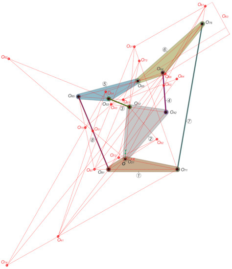
Figure 7. All rotation centers of an eight-bar “double-butterfly” planar linkage.

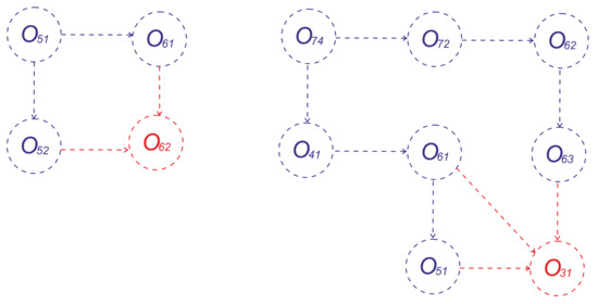
Figure 8. Subgraphs of secondary rotation centers required to solve the “double-butterfly” indeterminate planar linkage.

5. Proof of the Method

This short section presents constructive proof of the method. It should be noted that the number of IRCs is finite, and it is given by:

$$N=\frac{n(n-1)}{2},$$

where N is the number of IRCs, and n is the number of links in the linkage. Since both linkages have eight links, the number of IRCs is also, in both cases, twenty-eight.

• The single-butterfly linkage has nine primary centers. Two additional centers can be obtained by a straightforward application of the Aronhold–Kennedy theorem, $O_{31}$, and $O_{42}$. During the two-step process, the location of the following IRCs, $O_{62}$, $O_{64}$, $O_{72}$, $O_{73}$, $O_{82}$, $O_{83}$, and $O_{84}$, are found. Hence, after the process, the users will know the location of 18 out of 28 centers.
• The double-butterfly has 10 primary centers. During the two-step process, the location of the following IRCs, $O_{31}$, $O_{41}$, $O_{51}$, $O_{52}$, $O_{61}$, $O_{62}$, $O_{63}$, $O_{72}$, and $O_{74}$, are found. Hence, after the process, the users will know the location of 19 out of 28 centers.

Any person with some familiarity with the graphical techniques of the Aronhold–Kennedy theorem would recognize that, most likely, the location of the remaining IRC can be determined by the simple application of the Aronhold–Kennedy theorem. Even if this is not the case, the process can be repeated by choosing another secondary center. The location of all IRCs will be finished after a finite, usually small—no more than two- or three-steps—process. (In the examples shown in this contribution, it was possible to determine all the IRCs. There was no need to repeat the process.)

6. Conclusions

This paper introduced a novel and simpler method to obtain the secondary instantaneous centers of rotation of indeterminate planar linkages. The method only requires the solution and comparison of two quadratic equations or a quadratic equation and a cubic equation. They are simpler than the previous works reported in the literature. In addition, the method does not require the construction of the complete graph of the secondary IRCs, as indicated by Kung and Wang [14]. Motivated by the reviewers’ comments, the authors will embark in the search of a method applicable to indeterminate linkages containing gear pairs and up to 10 links. Finally, the results were verified by carrying out the velocity analyses of the linkages involved and by simulation using Adams©. The verification is not included here due to space considerations. However all the details are included in the M.Sc. thesis of the first author [24].

References

- Aronhold, S. Gründzuge der Kinematischen Geometrie. Verh. Ver. Z. Beförderung des Gewerbefleiss Preuss. 1872, 51, 129–155. [Google Scholar]
- Kennedy, A.B.W. The Mechanics of Machinery; Macmillan: London, UK, 1886; pp. 60–83. [Google Scholar]
- Shigley, J.E.; Uicker, J.J., Jr. Theory of Machines and Mechanisms; McGraw-Hill Inc.: Singapore, 1980. [Google Scholar]
- Klein, A.W. Kinematics of Machinery; Mc-Graw Hill Book Co.: New York, NY, USA, 1917. [Google Scholar]
- Modrey, J. Analysis of Complex Kinematic Chains with Influence Coefficients. J. Appl. Mech. 1959, 26, 184–188. [Google Scholar] [CrossRef]
- Goodman, T.P. Discussion to the paper Analysis of Complex Kinematic Chains with Influence Coefficients. J. Appl. Mech. 1960, 27, 215–216. [Google Scholar] [CrossRef][Green Version]
- Yan, H.S.; Hsu, M.H. An Analytical Method for Locating Instantaneous Velocity Centers. In DE-Vol.47 Flexible Mechanisms, Dynamics and Analysis, Proceedings of the ASME 1992 Design Technical Conferences, 22nd Biennial Mechanisms Conference, Scottsdale, AZ, USA, 13–16 September 1992; Kinzel, G., Reinholtz, C., Eds.; ASME: New York, NY, USA, 1992; pp. 353–359. [Google Scholar]
- Kim, M.; Han, M.S.; Seo, T.; Lee, J.W. A new instantaneous centers analysis methodology for planar closed chains via graphical representation. Int. J. Control Autom. Syst. 2016, 14, 1528–1534. [Google Scholar] [CrossRef]
- Valderrama-Rodríguez, J.I.; Rico, J.M.; Cervantes-Sánchez, J.J. A general method for the determination of the instantaneous screw axes of one-degree-of-freedom spatial mechanisms. Mech. Sci. 2020, 11, 91–99. [Google Scholar] [CrossRef]
- Di Gregorio, R. A novel method for the singularity analysis of planar mechanisms with more than one degree of freedom. Mech. Mach. Theory 2009, 44, 83–102. [Google Scholar] [CrossRef]
- Zarkandi, S. Application of mechanical advantage and instant centers on singularity analysis of single-DOF planar mechanisms. Trans. Mech. Eng. Div. Inst. Eng. Bangladesh 2010, 41, 50–57. [Google Scholar] [CrossRef][Green Version]
- Foster, D.E.; Pennock, G.R. Graphical methods to locate the secondary instant centers of single-degree-of-freedom indeterminate linkages. J. Mech. Des. 2003, 125, 268–274. [Google Scholar] [CrossRef]
- Di Gregorio, R. An algorithm for analytically calculating the positions of the secondary instant centers of indeterminate linkages. J. Mech. Des. 2008, 130, 1–9. [Google Scholar] [CrossRef]
- Kung, C.M.; Wang, L.C.T. Analytical method for locating the secondary instant centers of indeterminate planar linkages. Proc. Inst. Mech. Eng. Part C J. Mech. Eng. Sci. 2009, 223, 491–502. [Google Scholar] [CrossRef]
- Chang, Y.P.; Her, C. Locating instant centers of kinematically indeterminate linkages. J. Mech. Des. 2008, 130, 062304. [Google Scholar] [CrossRef]
- Liu, Z.; Chang, Y.P. The virtual cam method application and verification on locating key instant centers of ten-bars 1-DOF indeterminate linkages. In Proceedings of the ASME 2017 International Mechanical Engineering Congress and Exposition, Tampa, FL, USA, 3–9 November 2017; ASME: New York, NY, USA, 2017. [Google Scholar]
- Liu, Z.; Chang, Y.P. The virtual cam-hexagon method authentication on locating key instant centers of all planar single degree of freedom kinematically indeterminate linkages up to ten-bar. In Proceedings of the ASME 2019 International Mechanical Engineering Congress and Exposition, Pittsburgh, PA, USA, 9–15 November 2017; ASME: New York, NY, USA, 2017. [Google Scholar]
- Valderrama-Rodríguez, J.I.; Rico, J.M.; Cervantes-Sánchez, J.J. A screw theory approach to compute instantaneous rotation axes of indeterminate spherical linkages. Mech. Based Des. Struct. Mach. 2020, 1–41. [Google Scholar] [CrossRef]
- Ball, R.S. A Treatise on the Theory of Screws; Cambridge University Press: Cambridge, UK, 1900. [Google Scholar]
- Rico, J.M.; Gallardo-Alvarado, J.; Duffy, J. Screw theory and higher order kinematic analysis of open serial and closed chains. Mech. Mach. Theory 1999, 34, 559–586. [Google Scholar] [CrossRef]
- Brand, L. Vector and Tensor Analysis; John Wiley and Sons: New York, NY, USA, 1947. [Google Scholar]
- Rico, J.M.; Duffy, J. Orthogonal spaces and screw systems. Mech. Mach. Theory 1992, 27, 451–458. [Google Scholar] [CrossRef]
- Zhang, L.; Zhao, Y.; Ren, J. Screw rolling between moving and fixed axodes traced by lower-mobility parallel mechanism. Mech. Mach. Theory 2021, 163, 104354. [Google Scholar] [CrossRef]
- Valderrama-Rodríguez, J.I. Localización de los Ejes de Tornillos Instantáneos de Mecanismos Espaciales y sus Aplicaciones. Master’s Thesis, Universidad de Guanajuato, Guanajuato, Mexico, December 2018. [Google Scholar]
Publisher’s Note: MDPI stays neutral with regard to jurisdictional claims in published maps and institutional affiliations. |
© 2021 by the authors. Licensee MDPI, Basel, Switzerland. This article is an open access article distributed under the terms and conditions of the Creative Commons Attribution (CC BY) license (https://creativecommons.org/licenses/by/4.0/).