Subradiance Generation in a Chain of Two-Level Atoms with a Single Excitation

Abstract

Studies of subradiance in a chain N two-level atoms in the single excitation regime focused mainly on the complex spectrum of the effective Hamiltonian, identifying subradiant eigenvalues. This can be achieved by finding the eigenvalues N of the Hamiltonian or by evaluating the expectation value of the Hamiltonian on a generalized Dicke state, depending on a continuous variable k. This has the advantage that the sum above N can be calculated exactly, such that N becomes a simple parameter of the system and no longer the size of the Hilbert space. However, the question remains how subradiance emerges from atoms initially excited or driven by a laser. Here we study the dynamics of the system, solving the coupled-dipole equations for N atoms and evaluating the probability to be in a generalized Dicke state at a given time. Once the subradiant regions have been identified, it is simple to see if subradiance is being generated. We discuss different initial excitation conditions that lead to subradiance and the case of atoms excited by switching on and off a weak laser. This may be relevant for future experiments aimed at detecting subradiance in ordered systems.

1. Introduction

Since the seminal paper by Dicke [1], collective spontaneous emission by an ensemble of two-level atoms has been studied by many authors [2,3,4]. In particular subradiance, i.e., inhibited emission due to destructive interference between the emitters, has recently received great attention, both in disordered systems, as in a cloud [5,6,7,8], and in ordered systems, as in atomic chains or 2D and 3D lattices [9,10,11,12,13,14]. The theoretical studies on subradiance have been focused mostly on the study of the eigenvalues of the system [15,16] and in particular on the collective decay rate, which for subradiance is less than the single-atom decay $\Gamma$.

In disordered systems, subradiance has been investigated numerically and experimentally by switching off a continuous detuned laser driving a thermal cloud and calculating the decay rate of the fluorescence light intensity by reporting it in a semi-log plot [5,6,17]. After the initial fast decay, subradiance manifests itself in a slowly decaying fluorescence intensity with a rate below the single-atom decay rate. As a consequence of the existence of a single super-radiant mode and many degenerate subradiant modes, at first the subradiant decay is not purely exponential, since several modes decay simultaneously. For longer times, it then ends up with a pure exponential decay (referred as subradiant decay) when only one long-lived mode dominates. A similar approach can be adopted for ordered systems, such as atoms in a linear chain. Such linear chains have been investigated theoretically by different authors [18,19,20,21,22,23,24,25]. In the single-excitation approximation, subradiance has been studied in the previous literature by calculating the eigenvalues of the system, determined numerically by diagonalizing the finite $N\times N$ matrix associated with the Green operator describing the coupling between the emitters.

Recently, we proposed a different method to study subradiance in a finite linear chain, based on the evaluation of the expectation value of the effective Hamiltonian on a generalized Dicke state, depending on a continuous variable k [14]. This has several advantages: (1) it allows the collective decay rate $\Gamma \left(k\right)$ to be calculated as a function of a continuous parameter, mimicking the exact Fourier spectrum; (2) the sum over N can be calculated exactly, making N a mere parameter of the system and no longer the dimension of the matrix whose eigenvalues are to be evaluated; (3) the study of $\Gamma \left(k\right)$ allows us to identify the subradiant regions of the spectrum. The last point is important, because it can be used to detect how subradiance may be dynamically generated.

In general, little attention has been devoted to the generation of subradiance, from the preparation of the excited atoms or when the atoms are driven by a laser. There are a few exceptions, for instance, ref. [12], where the cooperative subradiant response of a two-dimensional square array of atoms in an optical lattice has been observed. Other experimental demonstrations of subradiance have been reported in [8,26,27]. A detailed description of methods commonly employed to analyze the cooperative responses of atomic arrays and an exploration of some recent developments and potential future applications of planar arrays is contained in ref. [25]. The long subradiant lifetimes may be used for storage and retrieval of quantum information [10,28] and other photonic devices, for instance, nanolasers [29], plasmonic ring nanocavities [30], and ultracold molecules [31].

By solving the coupled-dipole equations for N atoms with given initial conditions or in the presence of a driving laser, it is possible to project the solution at a given time on the generalized Dicke state. The result gives the probability distribution of the state as a function of the continuous variable k. Then, by identifying the subradiant regions of the spectrum, it is possible to see if subradiance has been generated. In particular, we find which is the initial state maximally generating subradiance: this is useful in order to understand the symmetry properties of the subradiant state.

We assume here an ideal chain. In a real experiment, fluctuations in the atomic position may be detrimental for cooperative effects [32,33]. For instance, the role of imperfections of the collective decay in a 1D array has been studied in ref. [23], showing that these phenomena are robust to realistic experimental imperfections.

This paper is organized as follows. In the first part we review the main results of ref. [14], defining the generalized Dicke state and adding the calculation of the collective frequency shift, both in the scalar and vectorial models. The second part is devoted to the generation of subradiance by suitable initial atomic excitations or when atoms are excited by a weak laser field. The dynamics of the system is investigated by solving the N coupled-dipole equations and projecting the single-particle state at the time t over the generalized Dicke state. We show that it is possible to build a maximally subradiant state, which in the limit of an infinite chain gives a vanishing spontaneous decay rate. Finally, we interpret the results in terms of the fluorescence intensity spatial distribution.

2. Modeling Emission from a Chain of Atoms with a Single Excitation

Here we define the collective frequency shift and decay rate as the real and imaginary part of the expectation value of the effective Hamiltonian over the generalized Dicke state. Preliminary results have been previously reported in ref. [14]. The calculations are carried out first for the scalar model and then extended to the vectorial model in Section 2.6.

2.1. Scalar Model

We consider N two-level atoms with ground state $|g_j⟩$ and excited state $|e_j⟩$ ($j=1,\dots ,N$), with atomic transition frequency ${\omega }_0=c{k}_0$, linewidth $\Gamma$, dipole $\mu$, and position ${\mathbf{r}}_j$. We consider here the single-excitation effective Hamiltonian in the scalar approximation [34,35]:

$$\begin{array}{ccc}\hfill \widehat{H}& =& -i{\displaystyle \frac{\hslash }{2}}\sum _{j,m}{G}_{jm}{\widehat{\sigma }}_j^{†}{\widehat{\sigma }}_m,\hfill \end{array}$$

(1)

where ${\widehat{\sigma }}_j=|g_j⟩⟨e_j|$ and ${\widehat{\sigma }}_j^{†}=|e_j⟩⟨g_j|$ are the lowering and raising operators, $G_{jm}$ is the scalar Green function,

$$G_{jm}=\left\{\begin{array}{cc}{\Gamma }_{jm}-i{\Omega }_{jm}\hfill & \mathrm{if}j\ne m,\hfill \\ \Gamma \hfill & \mathrm{if}j=m,\hfill \end{array}\right.$$

(2)

and

$${\Gamma }_{jm}=\Gamma {\displaystyle \frac{\sin \left(k_0{r}_{jm}\right)}{k_0{r}_{jm}}},{\Omega }_{jm}=\Gamma {\displaystyle \frac{\cos \left(k_0{r}_{jm}\right)}{k_0{r}_{jm}}},$$

(3)

where $r_{jm}=|{\mathbf{r}}_j-{\mathbf{r}}_m|$. ${\Gamma }_{jm}$ can be obtained as the angular average of the radiation field propagating between the two atomic positions ${\mathbf{r}}_j$ and ${\mathbf{r}}_m$ with wave-vector $\mathbf{k}=k_0(\sin \theta \cos \varphi ,\sin \theta \sin \varphi ,\cos \theta )$ (see Appendix A),

$${\Gamma }_{jm}={\displaystyle \frac{\Gamma }{2}}{⟨e^{-i\mathbf{k}·({\mathbf{r}}_j-{\mathbf{r}}_m)}+\mathrm{c}.\mathrm{c}.⟩}_{\Omega }$$

(4)

where the angular average is defined as

$${⟨f(\theta ,\varphi )⟩}_{\Omega }={\displaystyle \frac{1}{4\pi }}{\int }_0^{2\pi }d\varphi {\int }_0^{\pi }\sin \theta f(\theta ,\varphi )d\theta .$$

Equation (4) provides a simple interpretation of ${\Gamma }_{jm}$ as the coupling between the jth atom and the mth atom, mediated by the photon shared between the two atoms and averaged over all the vacuum modes. Equation (4) allows ${\Gamma }_{jm}$ to be factorized into the product of two terms, before averaging them over the total solid angle.

We consider N atoms placed along a linear chain with lattice constant d, with ${\mathbf{r}}_j=d(j-1){\widehat{\mathbf{e}}}_z$, with $j=1,\dots ,N$, so that Equation (4) becomes

$${\Gamma }_{jm}={\displaystyle \frac{\Gamma }{4}}{\int }_0^{\pi }\sin \theta \left[e^{-i{k}_{0}d(j-m)\cos \theta }+\mathrm{c}.\mathrm{c}.\right]d\theta .$$

(5)

2.2. Generalized Dicke State

We define the generalized Dicke states [14]:

$$|k⟩={\displaystyle \frac{1}{\sqrt{N}}}\sum _{j=1}^N{e}^{ikd(j-1)}|j⟩$$

(6)

where $|j⟩=|g_1,\dots ,e_j,\dots ,g_N⟩$ and $k\in (-\pi /d,\pi /d)$. This includes for $k=0$ the Dicke state [1] and for $k=k_0$ the timed Dicke state introduced by Scully [36,37]. It satisfies the completeness relation

$${\displaystyle \frac{d}{2\pi }}{\int }_{-\pi /d}^{\pi /d}dk|k⟩⟨k|=1.$$

(7)

As expected, the states $|k⟩$ are not orthogonal for a finite chain, since

$$⟨k^{\prime }|k⟩={\displaystyle \frac{\sin [(k-k^{\prime })dN/2]}{\sin [(k-k^{\prime })d/2]}}{e}^{i(k-k^{\prime })d(N-1)/2},$$

(8)

but they become so for an infinite chain, $⟨k^{\prime }|k⟩\to \delta (k-k^{\prime })$ for $N\to \infty$. So the states $|k⟩$ form an over-completed basis for the single-excitation manifold.

Notice that it is possible to extend the definition of the generalize Dicke state (6) to multi-excitation manifolds. Then, the approach described in the next sections can be straightforwardly extended to the multi-excitation modes. For instance, a two-excitation generalized Dicke state may be defined as

$$|k_1,k_2⟩=\mathcal{C}\sum _{j=1}^N\sum _{{\displaystyle \genfrac{}{}{0pt}{}{m=1}{m\ne j}}}^N{e}^{i{k}_{1}d(j-1)+i{k}_{2}d(m-1)}|j,m⟩$$

(9)

where $|j,m⟩=|g_1,\dots ,e_j,\dots ,e_m,\dots ,g_N⟩$ and $\mathcal{C}$ is a normalization constant. Preliminary results about two-excitation modes have been discussed in ref. [11].

2.3. Collective Frequency Shift and Decay Rate

Taking the expectation value of the effective Hamiltonian (1) over the generalized Dicke state (6) yields

$$-{\displaystyle \frac{2}{\hslash }}⟨k|\widehat{H}|k⟩={\Omega }_N\left(k\right)+i{\Gamma }_N\left(k\right)$$

(10)

where

$${\Omega }_N\left(k\right)={\displaystyle \frac{1}{N}}\sum _{j=1}^N\sum _{{\displaystyle \genfrac{}{}{0pt}{}{m=1}{m\ne j}}}^N{\Omega }_{jm}{e}^{ikd(j-m)}$$

(11)

is the collective frequency shift and

$${\Gamma }_N\left(k\right)={\displaystyle \frac{1}{N}}\sum _{j=1}^N\sum _{m=1}^N{\Gamma }_{jm}{e}^{ikd(j-m)}$$

(12)

is the collective decay rate. By using Equation (5) in Equation (12), we can write

$$\begin{array}{ccc}\hfill {\Gamma }_N\left(k\right)& =& {\displaystyle \frac{\Gamma }{2N}}{\int }_0^{\pi }\sin \theta {\left|F_k\left(\theta \right)\right|}^{2}d\theta \hfill \end{array}$$

(13)

where

$$\begin{array}{ccc}\hfill |F_k{\left(\theta \right)|}^2& =& {\left|\sum _{j=1}^N{e}^{i(k-k_0\cos \theta )d(j-1)}\right|}^2={\displaystyle \frac{{\sin }^2[(k-k_0\cos \theta )dN/2]}{{\sin }^2[(k-k_0\cos \theta )d/2]}}\hfill \end{array}$$

(14)

and

$$\begin{array}{ccc}\hfill {\Gamma }_N\left(k\right)& =& {\displaystyle \frac{\Gamma }{k_{0}dN}}{\int }_{(k-k_0)d/2}^{(k+k_0)d/2}{\displaystyle \frac{{\sin }^2\left(Nt\right)}{{\sin }^{2}t}}dt\hfill \end{array}$$

(15)

where we have changed the integration variable from $\theta$ to $t=(k-k_0\cos \theta )d/2$. For a large N, we can approximate in the integral of Equation (15),

$${\displaystyle \frac{{\sin }^2\left(Nt\right)}{{\sin }^{2}t}}\approx N^2\sum _{m=-\infty }^{+\infty }{\mathrm{sinc}}^2\left[\left(t-m\pi \right)N\right],$$

(16)

where $\mathrm{sinc}\left(x\right)=\sin x/x$, so that

$$\begin{array}{ccc}\hfill {\Gamma }_N\left(x\right)& =& ={\displaystyle \frac{\Gamma N}{a}}\sum _{m=-\infty }^{+\infty }{\int }_{(x-a)/2}^{(x+a)/2}{\mathrm{sinc}}^2\left[\left(t-m\pi \right)N\right]dt.\hfill \end{array}$$

(17)

where $a=k_{0}d$ and $x=kd$, with $x\in (-\pi ,\pi )$. Hence, we have transformed the double sum in Equation (12) into an integral, where N plays the role of a simple parameter of the system. The collective frequency shift takes the form

$${\Omega }_N\left(x\right)={\displaystyle \frac{\Gamma }{N}}\sum _{j=1}^N\sum _{{\displaystyle \genfrac{}{}{0pt}{}{m=1}{m\ne j}}}^N{\displaystyle \frac{\cos \left(a\right[j-m\left|\right)}{a|j-m|}}{e}^{ix(j-m)}.$$

(18)

2.4. Infinite Chain

If the chain is infinite, $N\to \infty$, the solution for the collective decay rate is

$$\begin{array}{ccc}\hfill {\Gamma }_{\infty }\left(x\right)& =& {\displaystyle \frac{\Gamma \pi }{a}}\sum _{m=-\infty }^{+\infty }\Pi [2m\pi -a<x<2m\pi +a]\hfill \end{array}$$

(19)

where $\Pi (a<x<b)$ is the rectangular function, equal to 1 for $a<x<b$ and 0 elsewhere. In the first Brillouin zone, $m=0$, ${\Gamma }_{\infty }\left(x\right)=\Gamma \pi /a$ for $\left|x\right|<a$ and ${\Gamma }_{\infty }\left(x\right)=0$ for $a<\left|x\right|<\pi$. Atomic modes in the region enclosed within the light line $k=\pm k_0$ are generally unguided and radiate into free space. Outside the light line ($\left|k\right|>k_0$), the modes are guided and subradiant, as the electromagnetic field is evanescent in the directions transverse to the chain. For an infinite chain, ${\lim }_{N\to \infty }{\Omega }_N\left(x\right)={\Omega }_{\infty }\left(x\right)$ depends only on the index $\mathcal{l}=j-m$,

$$\begin{array}{ccc}\hfill {\Omega }_{\infty }\left(x\right)& =& \Gamma \sum _{\mathcal{l}=-\infty }^{\infty }{\displaystyle \frac{\cos \left(a\right|\mathcal{l}\left|\right)}{a\left|\mathcal{l}\right|}}{e}^{ix\mathcal{l}}={\displaystyle \frac{\Gamma }{2a}}\sum _{\mathcal{l}=1}^{\infty }{\displaystyle \frac{1}{\mathcal{l}}}\left[e^{i(a+x)\mathcal{l}}+e^{i(a-x)\mathcal{l}}+\mathrm{c}.\mathrm{c}.\right].\hfill \end{array}$$

(20)

Using the expansion

$$\ln (1-z)=-\sum _{n=1}^{\infty }{\displaystyle \frac{z^n}{n}}$$

we write

$$\begin{array}{ccc}\hfill {\Omega }_{\infty }\left(x\right)& =& -{\displaystyle \frac{\Gamma }{2a}}\left\{\ln [1-e^{i(a+x)}]+\ln [1-e^{i(a-x)}]+\mathrm{c}.\mathrm{c}.\right\}\hfill \\ & =& -{\displaystyle \frac{\Gamma }{a}}\ln \left[2|\cos a-\cos x|\right]\hfill \end{array}$$

(21)

The frequency shift has a logarithmic divergence for $x=\pm a$ and three extremes at $x=0,\pm \pi$, with ${\Omega }_{\infty }\left(0\right)=-(2\Gamma /a)\ln \left[2\right|\sin (a/2)\left|\right]$ and ${\Omega }_{\infty }(\pm \pi )=-(2\Gamma /a)\ln \left[2\right|\cos (a/2)\left|\right]$, respectively.

2.5. Finite Chain

If the chain is finite, the collective decay rate ${\Gamma }_N\left(x\right)$ can be calculated by using Equation (17). The collective frequency shift of Equation (18) can be written by transforming the double sum into a single sum on the index $\mathcal{l}=j-m$, with a degenerate factor $g_{\mathcal{l}}=N-\mathcal{l}$:

$$\begin{array}{ccc}\hfill {\Omega }_N\left(x\right)& =& {\displaystyle \frac{2\Gamma }{N}}\sum _{\mathcal{l}=1}^{N-1}(N-\mathcal{l}){\displaystyle \frac{\cos \left(a\mathcal{l}\right)}{a\mathcal{l}}}\cos \left(x\mathcal{l}\right)\hfill \end{array}$$

(22)

2.6. Vectorial Model

We now extend the previous expressions to the vectorial model, taking into account the polarization of the electromagnetic field. The non-Hermitian Hamiltonian is now

$$\begin{array}{ccc}\hfill \widehat{H}& =& -i{\displaystyle \frac{\hslash }{2}}\sum _{\alpha ,\beta }\sum _{j,j^{\prime }}{G}_{\alpha ,\beta }({\mathbf{r}}_j-{\mathbf{r}}_{j^{\prime }}){\widehat{\sigma }}_{j,\alpha }^{†}{\widehat{\sigma }}_{j^{\prime },\beta }.\hfill \end{array}$$

(23)

where $\alpha ,\beta =(x,y,z)$. Here, ${\widehat{\sigma }}_{j,x}=({\widehat{\sigma }}_j^{m_J=1}+{\widehat{\sigma }}_j^{m_J=-1})/2$, ${\widehat{\sigma }}_{j,y}=({\widehat{\sigma }}_j^{m_J=1}-{\widehat{\sigma }}_j^{m_J=-1})/2i$, and ${\widehat{\sigma }}_{j,z}={\widehat{\sigma }}_j^{m_J=0}$, where ${\widehat{\sigma }}_j^{m_J}=|g_j⟩⟨e_j^{m_J}|$ is the lowering operator between the ground state $|g_j⟩$ and the three excited states $|e_j^{m_J}⟩$ of the jth atom with quantum numbers $J=1$ and $m_J=(-1,0,1)$. The vectorial Green function in Equation (23) is

$$G_{\alpha ,\beta }\left(\mathbf{r}\right)={\displaystyle \frac{3\Gamma }{2}}{\displaystyle \frac{e^{i{k}_{0}r}}{i{k}_{0}r}}\left[{\delta }_{\alpha ,\beta }-{\widehat{n}}_{\alpha }{\widehat{n}}_{\beta }+\left({\delta }_{\alpha ,\beta }-3{\widehat{n}}_{\alpha }{\widehat{n}}_{\beta }\right)\left({\displaystyle \frac{i}{k_{0}r}}-{\displaystyle \frac{1}{k_0^2{r}^2}}\right)\right]$$

(24)

with $r=\left|\mathbf{r}\right|$ and ${\widehat{n}}_{\alpha }$ being the components of the unit vector $\widehat{\mathbf{n}}=\mathbf{r}/r$. We consider the linear chain with lattice constant d, i.e., ${\mathbf{r}}_j=d(j-1){\widehat{\mathbf{e}}}_z$, with $j=1,\dots ,N$, and all the dipoles aligned with an angle $\delta$ with respect to the chain’s axis, so that ${\widehat{n}}_{\alpha }={\widehat{n}}_{\beta }=\cos \delta$ and

$$G^{\left(\delta \right)}\left(r_{jm}\right)={\displaystyle \frac{3\Gamma }{2}}{\displaystyle \frac{e^{i{k}_0{r}_{jm}}}{i{k}_0{r}_{jm}}}\left[{\sin }^2\delta +(1-3{\cos }^2\delta )\left({\displaystyle \frac{i}{k_0{r}_{jm}}}-{\displaystyle \frac{1}{k_0^2{r}_{jm}^2}}\right)\right]$$

(25)

where $r_{jm}=d|j-m|$. The decay rate for the vectorial model is given by the real part of $G^{\left(\delta \right)}\left(r_{jm}\right)$,

$$\begin{array}{ccc}\hfill {\Gamma }^{\left(\delta \right)}\left(r_{jm}\right)& =& {\displaystyle \frac{3\Gamma }{2}}\left[{\sin }^2\delta j_0\left(k_0{r}_{jm}\right)+(3{\cos }^2\delta -1){\displaystyle \frac{j_1\left(k_0{r}_{jm}\right)}{k_0{r}_{jm}}}\right]\hfill \end{array}$$

(26)

where $j_0\left(x\right)=\sin x/x$ and $j_1\left(x\right)=\sin x/x^2-\cos x/x$ are the spherical Bessel functions of orders $n=0$ and $n=1$. The frequency shift is given by the negative of the imaginary part of $G^{\left(\delta \right)}\left(r_{jm}\right)$,

$$\begin{array}{ccc}\hfill {\Omega }^{\left(\delta \right)}\left(r_{jm}\right)& =& {\displaystyle \frac{3\Gamma }{2}}\left[{\sin }^2\delta {\displaystyle \frac{\cos \left(k_0{r}_{jm}\right)}{k_0{r}_{jm}}}+(3{\cos }^2\delta -1)\left({\displaystyle \frac{\sin \left(k_0{r}_{jm}\right)}{{\left(k_0{r}_{jm}\right)}^2}}+{\displaystyle \frac{\cos \left(k_0{r}_{jm}\right)}{{\left(k_0{r}_{jm}\right)}^3}}\right)\right]\hfill \end{array}$$

(27)

We note that Equations (26) and (27) reduce to the expressions (3) of the scalar model for ${\cos }^2\delta =1/3$, i.e., for $\delta =54.73°$. Hence the scalar model, generally considered unrealistic for non-dilute systems, in a linear chain can be obtained for a particular orientation of the dipoles. As for the scalar model, we define a collective decay rate, ${\Gamma }_N^{\left(\delta \right)}\left(k\right)=-(2/\hslash )\mathrm{Im}⟨k|\widehat{H}|k⟩$, and a collective frequency shift, ${\Omega }_N^{\left(\delta \right)}\left(k\right)=-(2/\hslash )\mathrm{Re}⟨k|\widehat{H}|k⟩$, where $\widehat{H}$ is defined in Equation (23) and where now $|k⟩=(1/\sqrt{N}){\sum }_{j=1}^N{e}^{ikd(j-1)}|g_1,\dots ,e_j^{\left(\delta \right)},\dots ,g_N⟩$, where $|e_j^{\left(\delta \right)}⟩$ denotes the excited atoms with the combination of the Zeeman sublevels yielding the dipoles oriented with the angle $\delta$ with respect to the chain’s axis. It is possible to demonstrate that the collective decay rate is [14]

$$\begin{array}{ccc}\hfill {\Gamma }_N^{\left(\delta \right)}\left(x\right)& =& {\displaystyle \frac{3\Gamma N}{2a}}\sum _{m=-\infty }^{+\infty }{\int }_{(x-a)/2}^{(x+a)/2}\left[{\sin }^2\delta +{\displaystyle \frac{1}{2}}(1-3{\cos }^2\delta ){\displaystyle \frac{{(x-2t)}^2-a^2}{a^2}}\right]\hfill \\ & \times & {\mathrm{sinc}}^2\left[\left(t-m\pi \right)N\right]dt\hfill \end{array}$$

(28)

(where $x=kd$) while the collective frequency shift is

$$\begin{array}{ccc}\hfill {\Omega }_N^{\left(\delta \right)}\left(x\right)& =& {\displaystyle \frac{2}{N}}\sum _{\mathcal{l}=1}^{N-1}(N-\mathcal{l}){\Omega }^{\left(\delta \right)}\left(a\mathcal{l}\right)\cos \left(x\mathcal{l}\right).\hfill \end{array}$$

(29)

If the chain is infinite, $N\to \infty$,

$$\begin{array}{ccc}\hfill {\Gamma }_{\infty }^{\left(\delta \right)}\left(x\right)& =& {\displaystyle \frac{3\Gamma \pi }{2a}}\sum _{m=-\infty }^{+\infty }\left\{{\sin }^2\delta +{\displaystyle \frac{1}{2}}(1-3{\cos }^2\delta ){\displaystyle \frac{{(x-2\pi m)}^2-a^2}{a^2}}\right\}\hfill \\ & \times & \Pi [2m\pi -a<x<2m\pi +a],\hfill \end{array}$$

(30)

and

$$\begin{array}{ccc}\hfill {\Omega }_{\infty }^{\left(\delta \right)}\left(x\right)& =& 2\sum _{\mathcal{l}=1}^{\infty }{\Omega }^{\left(\delta \right)}\left(a\mathcal{l}\right)\cos \left(x\mathcal{l}\right)\hfill \\ & =& {\displaystyle \frac{3\Gamma }{2a^3}}\mathrm{Re}\left\{-a^2{\sin }^2\delta \left[\ln \left(1-e^{i(x+a)}\right)+\ln \left(1-e^{i(x-a)}\right)\right]+(3{\cos }^2\delta -1)\right.\hfill \\ & \times & \left.\left[-ia{\mathrm{Li}}_2\left(e^{i(x+a)}\right)+ia{\mathrm{Li}}_2\left(e^{i(x-a)}\right)+{\mathrm{Li}}_3\left(e^{i(x+a)}\right)+{\mathrm{Li}}_3\left(e^{i(x-a)}\right)\right]\right\}\hfill \end{array}$$

(31)

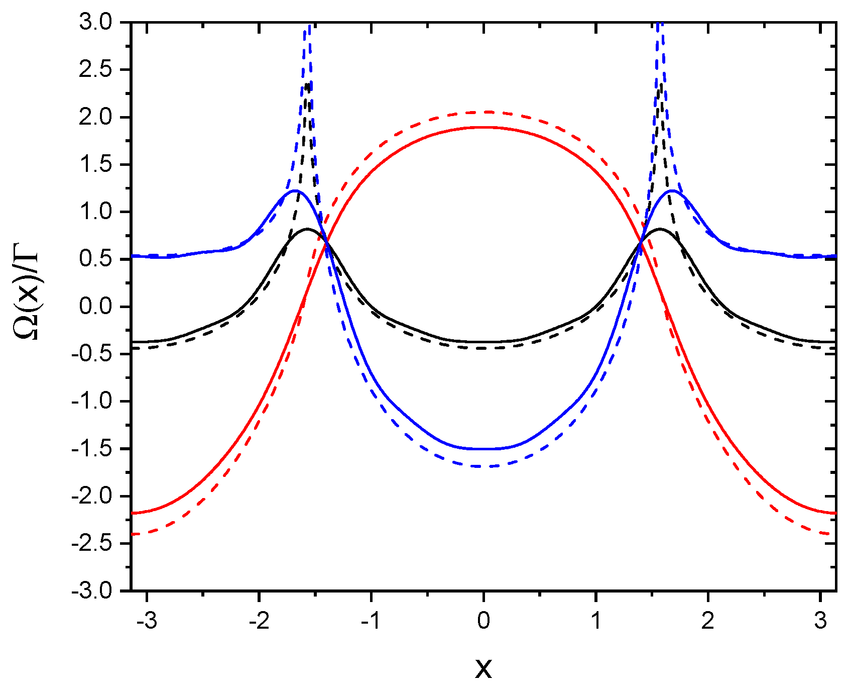
where ${\mathrm{Li}}_{\nu }\left(z\right)={\sum }_{\mathcal{l}=1}^{\infty }{z}^{\mathcal{l}}/{\mathcal{l}}^{\nu }$ is the PolyLog function. Figure 1 and Figure 2 show $\Gamma \left(x\right)/\Gamma$ and $\Omega \left(x\right)/\Gamma$ vs. x for $a=\pi /2$, for an infinite chain (dashed lines) and for a finite chain with $N=10$ (continuous lines). Black lines are for the scalar model, red and blue lines are for the vectorial model, with $\delta =0$ and $\delta =\pi /2$, respectively. For an infinite chain the collective decay rate is zero for $\left|x\right|>a$ (i.e., for $\left|k\right|>k_0$), both for the scalar and the vectorial model. Notice that for $\delta =0$ the phase shift ${\Omega }_{\infty }^{(\delta =0)}\left(x\right)$ is not diverging at $x=\pm a$.

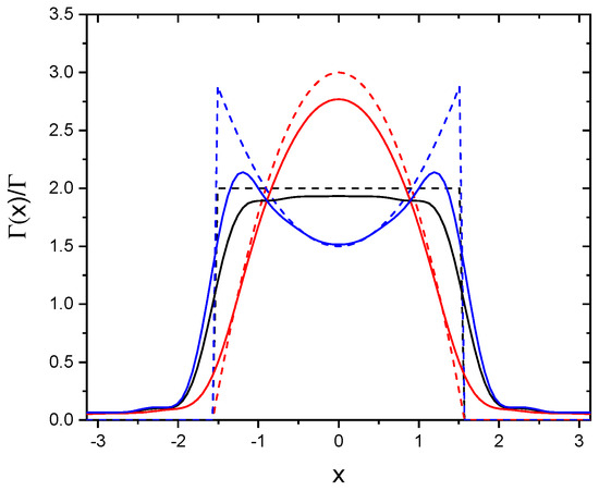
Figure 1. $\Gamma \left(x\right)/\Gamma$ vs. x for $a=\pi /2$. Dashed lines are for an infinite chain, continuous lines for a finite chain with $N=10$. Black lines are for the scalar model, red and blue lines for the vectorial model with $\delta =0$ and $\delta =\pi /2$, respectively.

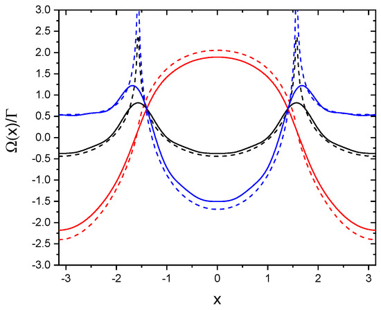
Figure 2. $\Omega \left(x\right)/\Gamma$ vs. x for $a=\pi /2$. Dashed lines are for an infinite chain, continuous lines for a finite chain with $N=10$. Black lines are for the scalar model, red and blue lines for the vectorial model with $\delta =0$ and $\delta =\pi /2$, respectively.

3. Dynamics

Having characterized the properties of the collective decay rate and frequency shift, identifying the subradiant zone $\left|x\right|>a$ where the collective decay rate is less than the single-atom decay rate $\Gamma$, we are interested now to study how subradiance can be generated by properly exciting the atoms. First, we define the probability distribution of the system to be in a given generalized Dicke state $|k⟩$, expressed in terms of the single-particle basis. Then we study the time evolution of this distribution, leading to subradiance. The following expressions are valid for both the scalar and vectorial model, so we omit the suffix $\left(\delta \right)$ where not necessary.

3.1. The Probability Density $P\left(k\right)$

Let us assume that the state of the system is $|\Psi ⟩=\alpha |g_1\dots g_N⟩+|{\Psi }^{\prime }⟩$, where

$$|{\Psi }^{\prime }⟩=\sum _{j=1}^N{\beta }_j|j⟩$$

(32)

describes the state in the single-excitation manifold. By projecting on the generalized Dicke basis (6),

$$|\Psi ⟩={\displaystyle \frac{d}{2\pi }}{\int }_{-\pi /d}^{\pi /d}dk|k⟩⟨k|{\Psi }^{\prime }⟩$$

(33)

where

$$⟨k|{\Psi }^{\prime }⟩={\displaystyle \frac{1}{\sqrt{N}}}\sum _{j=1}^N{e}^{-ikd(j-1)}{\beta }_j={\displaystyle \frac{1}{\sqrt{N}}}{A}_N\left(k\right).$$

(34)

Hence, the probability density to be in a state $|k⟩$ is

$$P\left(k\right)={\displaystyle \frac{dN}{2\pi }}{\displaystyle \frac{|⟨k|{\Psi }^{\prime }⟩{|}^2}{⟨{\Psi }^{\prime }|{\Psi }^{\prime }⟩}}={\displaystyle \frac{d}{2\pi }}{\displaystyle \frac{{\left|{\sum }_{j=1}^N{e}^{-ikd(j-1)}{\beta }_j\left(t\right)\right|}^2}{{\sum }_{j=1}^N{\left|{\beta }_j\right|}^2}}={\displaystyle \frac{|A_N{\left(k\right)|}^2}{{\int }_{-\pi /d}^{\pi /d}{\left|A_N\left(k\right)\right|}^{2}dk}}$$

(35)

with

$${\int }_{-\pi /d}^{\pi /d}P\left(k\right)dk=1.$$

(36)

Equation (35) expresses the probability density in terms of the dipole amplitudes of the single atoms, whose time evolution is described in the following section.

3.2. Dynamics of the Probability Density $P\left(k\right)$

Let us consider the time evolution of the atomic system in the presence of an external driving field in the scalar model. In the linear regime, the probability amplitudes ${\beta }_j\left(t\right)$ evolve with the following coupled-dipole equations:

$${\displaystyle \frac{d{\beta }_j}{dt}}=i{\Delta }_0{\beta }_j-i{\displaystyle \frac{{\Omega }_0}{2}}{e}^{ia(j-1)}-{\displaystyle \frac{\Gamma }{2}}\sum _{m=1}^N{G}_{jm}{\beta }_m$$

(37)

where $G_{jm}$ is defined in Equation (2), and $a=k_{0}d$, ${\Omega }_0$ and ${\Delta }_0$ are the Rabi frequency and the laser-atom detuning of the driving laser field. In the vectorial model and for dipoles all aligned with the same angle $\delta$ with respect to the chain’s axis, the probability amplitudes ${\beta }_j^{\left(\delta \right)}\left(t\right)$ evolve with the equations

$${\dot{\beta }}_j^{\left(\delta \right)}=\left(i{\Delta }_0-{\displaystyle \frac{\Gamma }{2}}\right){\beta }_j^{\left(\delta \right)}-i{\displaystyle \frac{{\Omega }_0^{\left(\delta \right)}}{2}}{e}^{ia(j-1)}-{\displaystyle \frac{1}{2}}\sum _{{\displaystyle \genfrac{}{}{0pt}{}{m=1}{m\ne j}}}^N{G}^{\left(\delta \right)}\left(a\right|j-m\left|\right){\beta }_m^{\left(\delta \right)}$$

(38)

where the driving field has the same polarization as the dipoles and $G^{\left(\delta \right)}\left(x\right)={\Gamma }^{\left(\delta \right)}\left(x\right)-i{\Omega }^{\left(\delta \right)}\left(x\right)$, where ${\Gamma }^{\left(\delta \right)}\left(x\right)$ and ${\Omega }^{\left(\delta \right)}\left(x\right)$ are defined in Equations (26) and (27). We notice that Equations (37) and (38) have the same form, the only difference being the expression of G. In the following we use the same notation for both the scalar and vectorial models.

From Equation (37), it is possible to obtain the equation for the temporal evolution of the probability amplitude $A_N(x,t)$ defined in Equation (34) (where $x=kd$) (see Appendix B):

$$\begin{array}{ccc}\hfill {\displaystyle \frac{\partial A_N(x,t)}{\partial t}}& =& \left(i{\Delta }_0-{\displaystyle \frac{\Gamma }{2}}\right)A_N(x,t)-i{\displaystyle \frac{{\Omega }_0}{2}}{\displaystyle \frac{\sin \left[\right(x-a)N/2]}{\sin \left[\right(x-a)/2]}}{e}^{-i(x-a)(N-1)/2}\hfill \\ & -& {\displaystyle \frac{\Gamma }{a}}\sum _{\mathcal{l}=1}^{N-1}\left[\sin \left(a\mathcal{l}\right)-i\cos \left(a\mathcal{l}\right)\right]{\displaystyle \frac{\cos \left(x\mathcal{l}\right)}{\mathcal{l}}}{A}_{N-\mathcal{l}}(x,t)\hfill \end{array}$$

(39)

For an infinite chain,

$$\underset{N\to \infty }{\lim }{\displaystyle \frac{\sin \left[\right(x-a)N/2]}{\sin \left[\right(x-a)/2]}}=2\pi \delta (x-a)$$

and

$$\begin{array}{ccc}\hfill {\displaystyle \frac{\partial A_{\infty }(x,t)}{\partial t}}& =& \left[i{\Delta }_0+i{\displaystyle \frac{{\Omega }_{\infty }\left(x\right)}{2}}-{\displaystyle \frac{{\Gamma }_{\infty }\left(x\right)}{2}}\right]A_{\infty }(x,t)-i\pi {\Omega }_0\delta (x-a)\hfill \end{array}$$

(40)

where ${\Gamma }_{\infty }$ and ${\Omega }_{\infty }$ are defined in Equations (19) and (21). The solution of Equation (40) is

$$\begin{array}{ccc}\hfill A_{\infty }(x,t)& =& A_{\infty }(x,0)e^{(i{\Delta }_0+i{\Omega }_{\infty }\left(x\right)/2-{\Gamma }_{\infty }\left(x\right)/2)t}\hfill \\ & +& {\displaystyle \frac{2\pi {\Omega }_0\delta (x-a)}{2{\Delta }_0+{\Omega }_{\infty }+i{\Gamma }_{\infty }}}\left(1-e^{(i{\Delta }_0+i{\Omega }_{\infty }\left(x\right)/2-{\Gamma }_{\infty }\left(x\right)/2)t}\right).\hfill \end{array}$$

(41)

4. Generation of Subradiance

Based on the previous expressions, we now discuss how subradiance can be generated, studying the temporal evolution from some initial conditions of the probability amplitudes ${\beta }_j$. The case of excitation by an incident laser field is discussed in Section 4.3.

4.1. Single Excited Atom

As a first example, we consider a chain of $N=100$ atoms with $a=\pi /2$, no driving laser, ${\Omega }_0=0$, and ${\Delta }_0=0$, and a single initially excited atom in the middle of the chain, with ${\beta }_{N/2}=1$ and all the others ${\beta }_j$ equal to zero. From Equation (35), the initial probability to be in the state $|x⟩$ is $P(x,0)=1/\left(2\pi \right)$ (where $x=kd$), i.e., it is uniform. Figure 3 shows $P(x,t)$ vs. x at different times, from $t=0$ until $t=10/\Gamma$, obtained by solving Equation (38) for $\delta =\pi /2$: after a few time units, the probability becomes zero for $\left|x\right|<a$ and different from zero in the subradiant interval $a<\left|x\right|<\pi$.

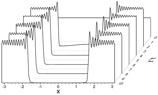
Figure 3. $P(x,t)$ vs. x for $\Gamma t=0,\dots ,10$, $a=\pi /2$, and $N=100$. Initially a single atom is excited in the middle of the chain; obtained from the vectorial model with $\delta =\pi /2$.

For an infinite chain, $|A_{\infty }{(x,t)|}^2=\exp [-{\Gamma }_{\infty }\left(x\right)t]$, where ${\Gamma }_{\infty }\left(x\right)=0$ for $a<\left|x\right|<\pi$. In the limit $t\to \infty$, $P(x,t)\to 0$ for $\left|x\right|<a$ and $P(x,t)\to {\displaystyle \frac{1}{2(\pi -a)}}$ for $a<\left|x\right|<\pi$. Figure 4 shows $P(x,t)$ at $t=10/\Gamma$ and $a=\pi /2$ (blue continuous line), obtained for the same parameters as in Figure 3, together with the value $P(x,\infty )=1/\left[2\right(\pi -a\left)\right]$ obtained for an infinite chain (dashed line).

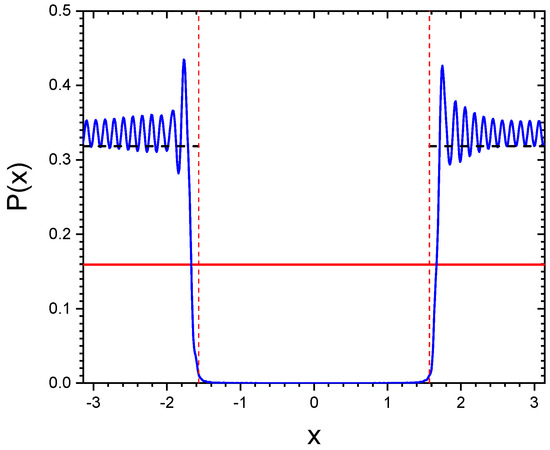
Figure 4. $P(x,t)$ vs. x (blue line) for $\Gamma t=10$ and the same parameters as in Figure 3. Initially a single atom is excited in the middle of the chain. The dashed line is the analytical result $P(x,\infty )=1/\left[2\right(\pi -a\left)\right]$ for an infinite chain, while the red line is the initial value $P(x,0)=1/2\pi$.

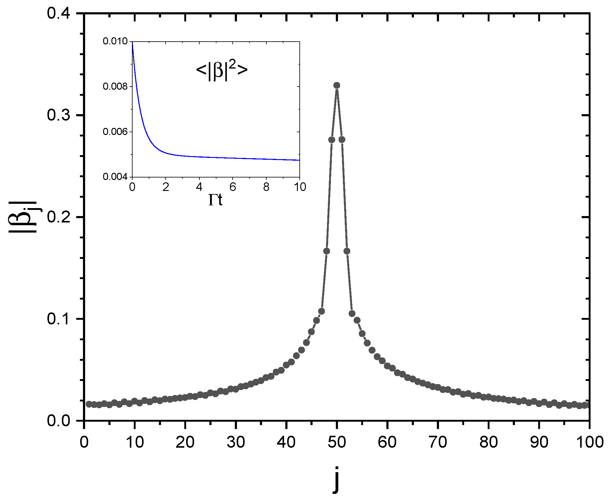
Hence, a single excited atom generates a subradiance state with a probability $P\left(x\right)$, which for an infinite chain is uniform in the subradiance spectral region $a<\left|x\right|<\pi$. It is interesting to see the distribution of the dipole amplitudes for the case in Figure 4: Figure 5 shows $|{\beta }_j|$ vs. j at $t=10/\Gamma$, where the inset shows the average excitation probability $⟨|\beta {|}^2⟩$ vs. time. We see the initial excitation for the atom with $j=N/2$ spreading among the adjacent atoms, to a final distribution generating subradiance. Although not visible in Figure 5, it is expected that the destructive interference among the atoms inhibits the spontaneous decay of the excitation, as discussed in the next section.

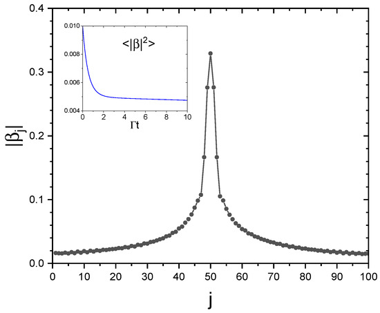
Figure 5. $|{\beta }_j|$ vs. j for $N=100$ and $a=\pi /2$, at $\Gamma t=10$, for the case of Figure 4. The inset shows the average excitation probability $⟨|\beta {|}^2⟩$ vs. time.

4.2. The Most Subradiant State

Since an initial uniform probability $P\left(x\right)$ generates asymptotically a subradiant distribution which is uniform for an infinite chain, as observed in the previous case, we are now interested in obtaining the values of ${\beta }_j$ which generate such a subradiant distribution. We assume

$$A_N\left(x\right)=e^{-ix(N/2-1)}\left\{\begin{array}{ccc}1\hfill & \mathrm{if}a<\hfill & \left|x\right|<\pi \hfill \\ 0\hfill & \mathrm{if}\hfill & \left|x\right|<a.\hfill \end{array}\right.$$

(42)

which describes a subradiant state, with zero probability distribution in the superradiant region $\left|x\right|<a$ and uniform distribution in the subradiant region $a<\left|x\right|<\pi$. Calculating the single-atom probability amplitude ${\beta }_j$, we obtain

$${\beta }_j={\displaystyle \frac{1}{2\pi }}{\int }_{-\pi }^{\pi }{e}^{ix(j-1)}{A}_N\left(x\right)dx=\left\{\begin{array}{ccc}1-{\displaystyle \frac{a}{\pi }}\hfill & \mathrm{if}\hfill & j={\displaystyle \frac{N}{2}}\hfill \\ \hfill & \\ -{\displaystyle \frac{\sin \left[a\right(j-N/2\left)\right]}{\pi (j-N/2)}}\hfill & \mathrm{if}\hfill & j\ne {\displaystyle \frac{N}{2}}\hfill \end{array}\right.$$

(43)

The ${\beta }_j$ defined in Equation (43) reproduces the distribution amplitude (42) only in the limit $N\to \infty$ (see Appendix C), since the states $|k⟩$ are not orthogonal. Figure 6 shows the probability density distribution $P(x,t)$ at $t=0$ (black dashed line) and at $\Gamma t=10$ (blue continuous line), obtained by solving Equation (38) with the initial condition (43), $N=100$, $a=\pi /2$, and $\delta =\pi /2$. For an infinite chain, $P\left(x\right)=1/\left[2\right(\pi -a\left)\right]$ for $a<\left|x\right|<\pi$ and zero for $\left|x\right|<a$, as obtained from Equation (42) (red line in Figure 7). Notice the similarities between Figure 4 for the single initially excited atom and Figure 6 for the initial state (43). We conclude that the state described by Equation (43) represents the ’most subradiant’ state for a finite chain of N atoms, with a purely subradiant spectrum in the limit of an infinite chain.

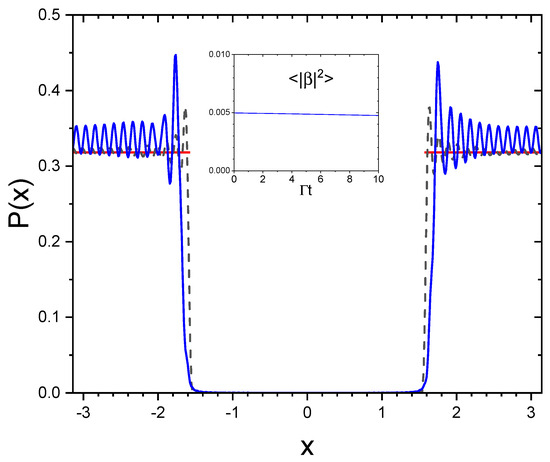
Figure 6. Probability density distribution $P(x,t)$ at $t=0$ (black dashed line) and at $\Gamma t=10$ (blue line), for $N=100$, $a=\pi /2$, and $\delta =\pi /2$, obtained by numerically solving Equation (37) with the initial condition (43). The red line is the case of an infinite chain. The inset shows that the average excitation probability $⟨|\beta {|}^2⟩$ is almost constant.

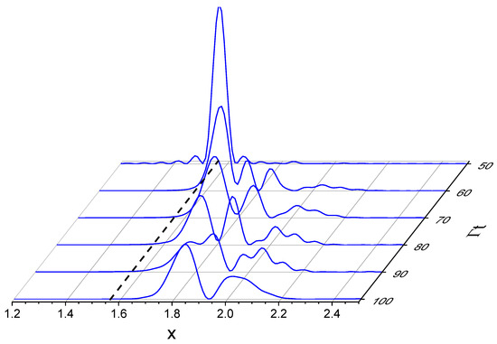
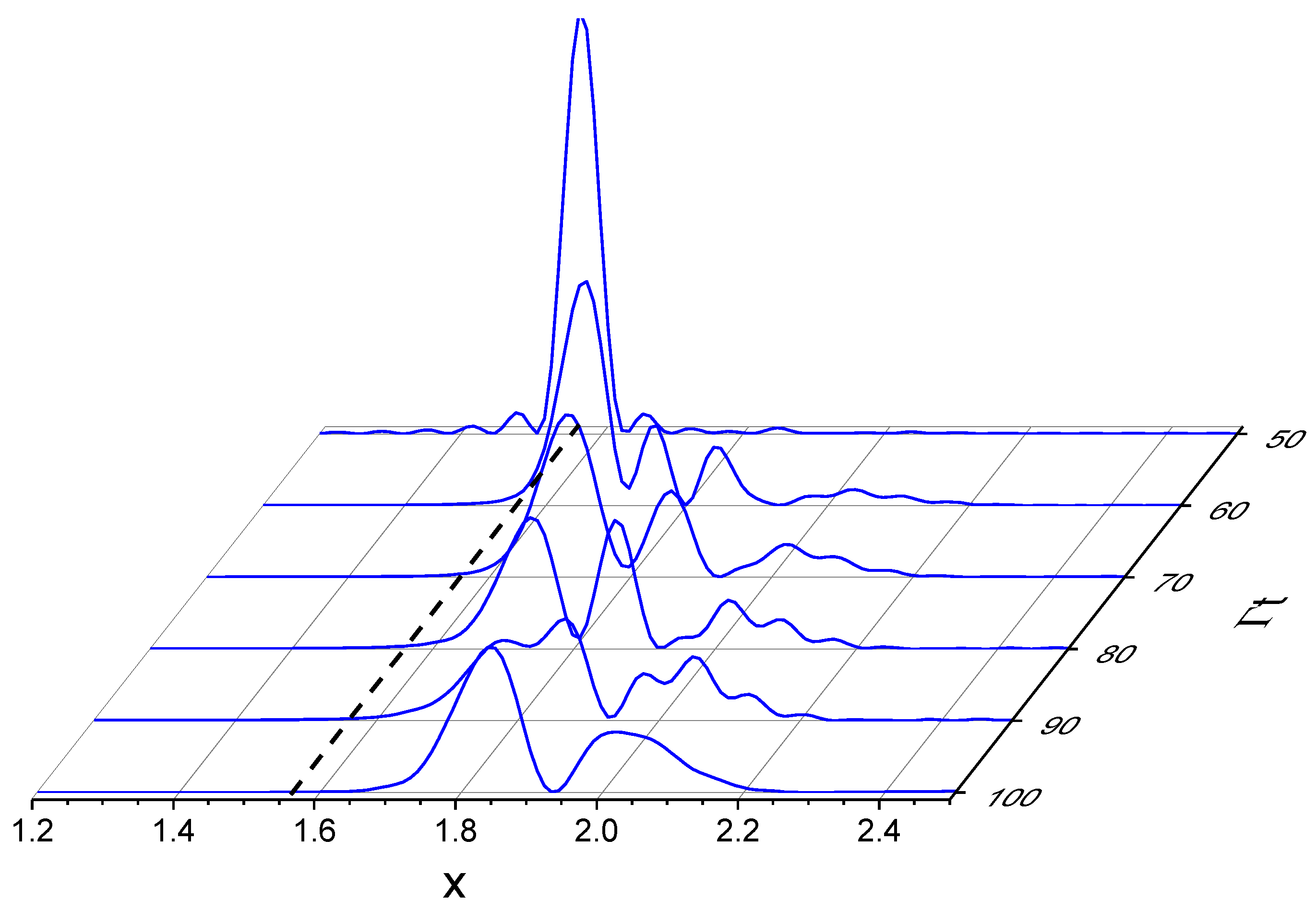
Figure 7. $P(x,t)$ vs. x at different times after the laser has been switched off, for a chain of $N=100$, $a=\pi /2$, and $\delta =\pi /2$, driven by a detuned laser with ${\Omega }_0=0.1\Gamma$ and ${\Delta }_0=10\Gamma$. The dashed line is the value $x=a$. The laser is switched off at $\Gamma t=50$.

4.3. Atoms Driven by a Laser

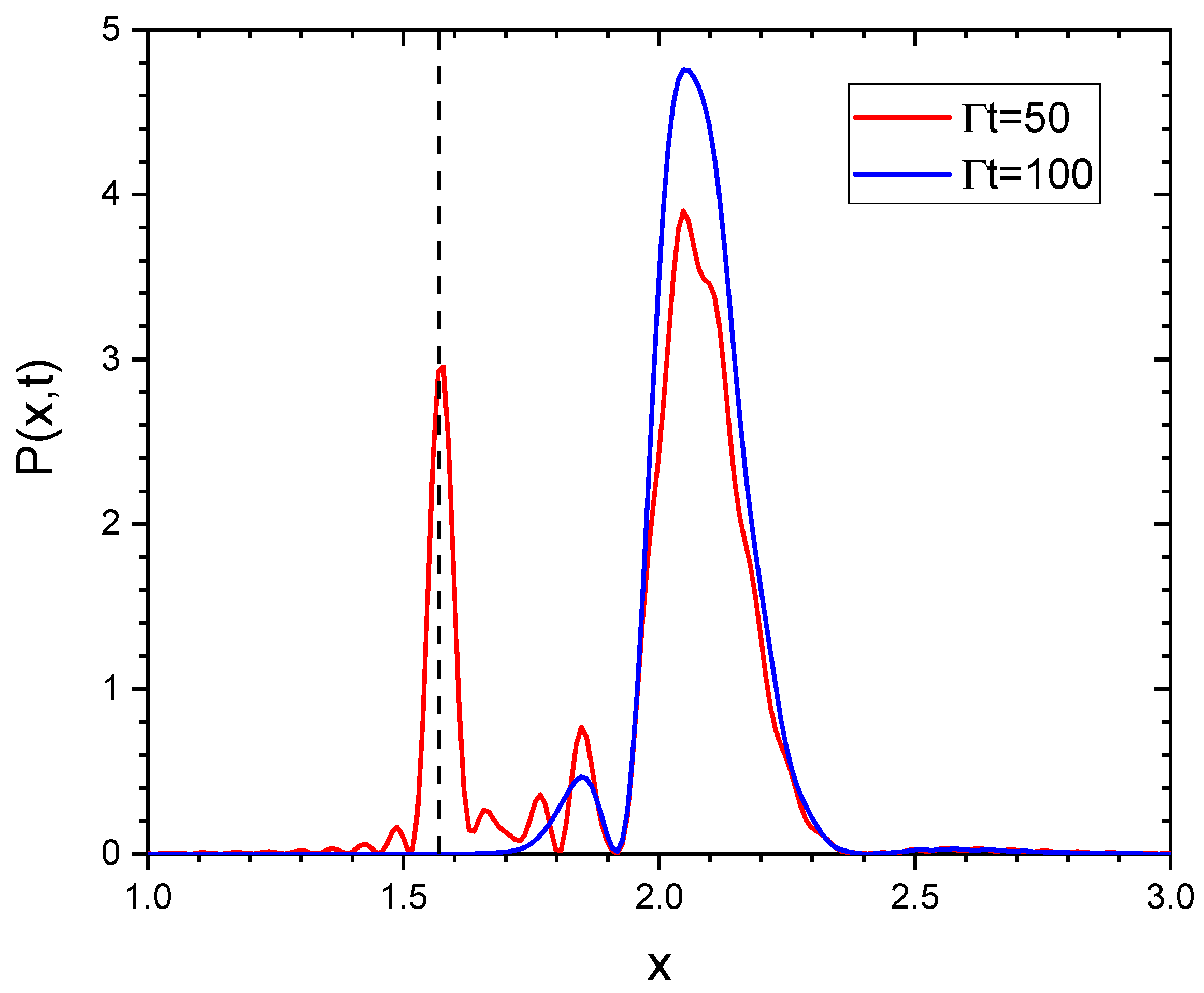
We now study the subradiance generation when the atoms are excited by an external laser field and then switched off. As an example, we consider a chain of $N=100$ atoms with $a=\pi /2$ and $\delta =\pi /2$, weakly driven by a detuned laser, with ${\Omega }_0=0.1\Gamma$ and ${\Delta }_0=10\Gamma$. The atoms, initially unexcited (i.e., ${\beta }_j\left(0\right)=0$ for $j=1,\dots ,N$), are driven by the laser up to $t_0=50/\Gamma$, after which the laser is switched off. Figure 7 shows $P(x,t)$ vs. x and at different times t after the laser is switched off, obtained by solving the vectorial model of Equation (38).

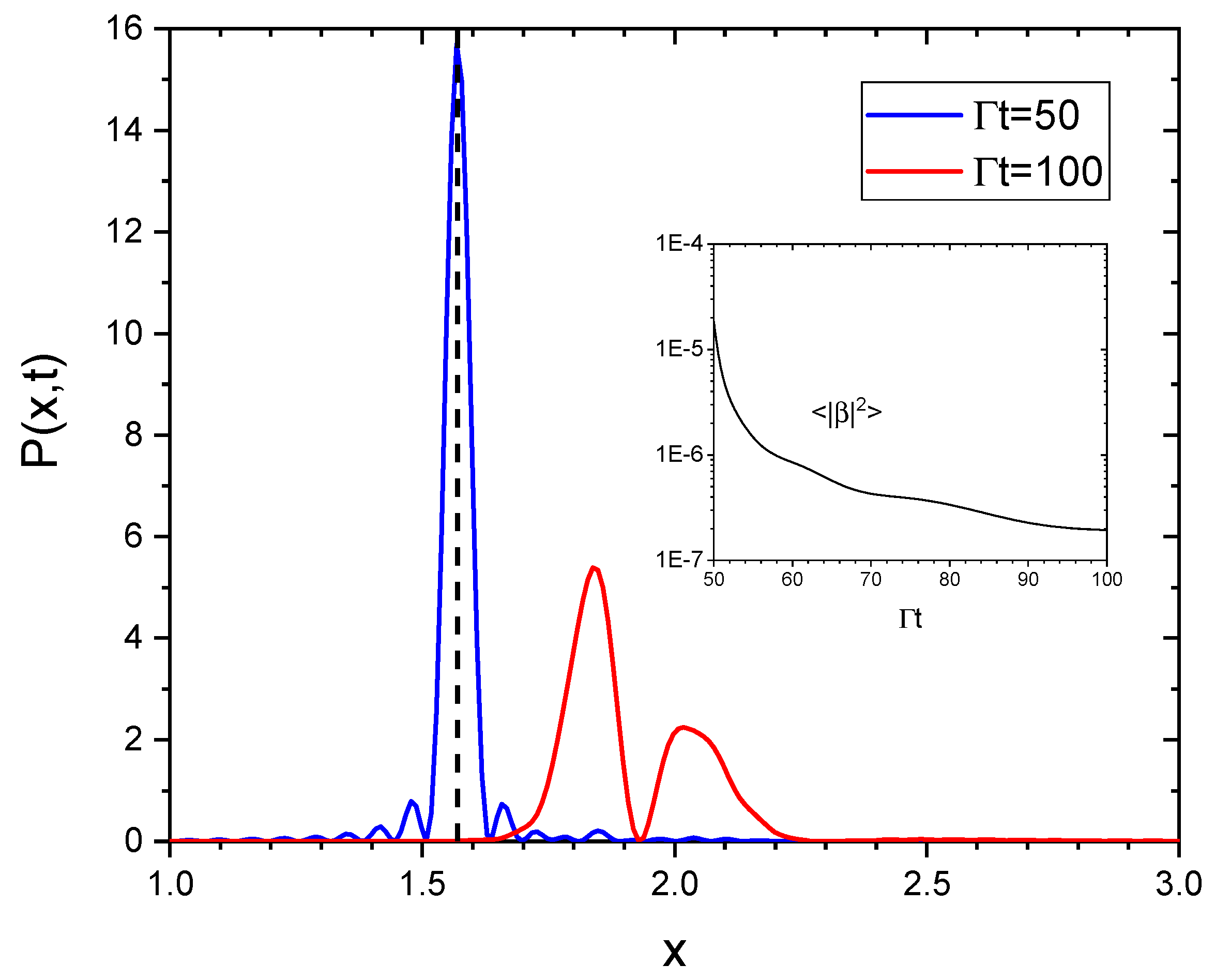
The distributions $P(x,t)$ at the laser switch-off time $t=50/\Gamma$ (blue continuous line) and at $t=100/\Gamma$ (red line) are shown in Figure 8; we see that the driving laser on brings the atoms close to a timed Dicke state, $|k_0⟩$ [36] (dashed line $x=a$ in Figure 8), with a width inversely proportional to the chain’s length $dN$. The inset of Figure 8 shows that, after the initial fast decay, subradiance manifests itself in a slow decay of the excitation. At first, the subradiant decay is not purely exponential, since several modes decay simultaneously. For longer times, it then ends up with a pure exponential decay when only one long-lived mode dominates. However, the precise evaluation of the decay rate can be problematic due to the general non-exponential decay. In our approach, we determine the precise distribution of the subradiant modes; as can be observed from the red line in Figure 8, at later times, after the laser switch-off, the distribution $P(x,t)$ is mostly in the subradiant region, $x>a$. The distribution is broad, so there is not a single subradiant mode dominating. As a consequence, the decay is not purely exponential.

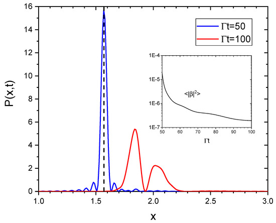
Figure 8. $P(x,t)$ vs. x at the switch-off time $\Gamma t=50$ (blue line) and at $\Gamma t=100$ (red line), for the same parameters as in Figure 8. The vertical dashed line indicates the value $x=a=\pi /2$. The black dashed line is at $x=a$. The inset shows the average excitation probability $⟨|\beta {|}^2⟩$ vs. time.

In the case of an infinite chain, Equation (41) gives

$$|A_{\infty }{(x,\infty )|}^2={\displaystyle \frac{2N{\left(\pi {\Omega }_0\right)}^2}{{(2{\Delta }_0+{\Omega }_{\infty })}^2+{\Gamma }_{\infty }^2}}\delta (x-a),$$

(44)

where we use the relation

$$\underset{N\to \infty }{\lim }{\displaystyle \frac{{\sin }^2[(x-a)N/2]}{{\sin }^2[(x-a)/2]}}=\pi N\delta (x-a).$$

Hence, for a driven infinite chain the asymptotic spectrum is $P(x,\infty )\propto \delta (x-a)$ and no subradiance occurs. To observe subradiance, we need a finite chain, as seen in Figure 7 and Figure 8; in the detuned case, the finite width of the driving term (second term on the right-hand side of Equation (39) and blue line in Figure 8) is proportional to $1/N$ and is responsible for the subradiant components of the spectrum until the laser is on; these subsequently evolve without reaching a steady-state value. From the above analysis, the possibility of having access to the full spectral distribution of the subradiant modes is clearly more advantageous than observing the time-decaying excitation to obtain the subradiant decay rate, as, for instance, in refs. [5,6].

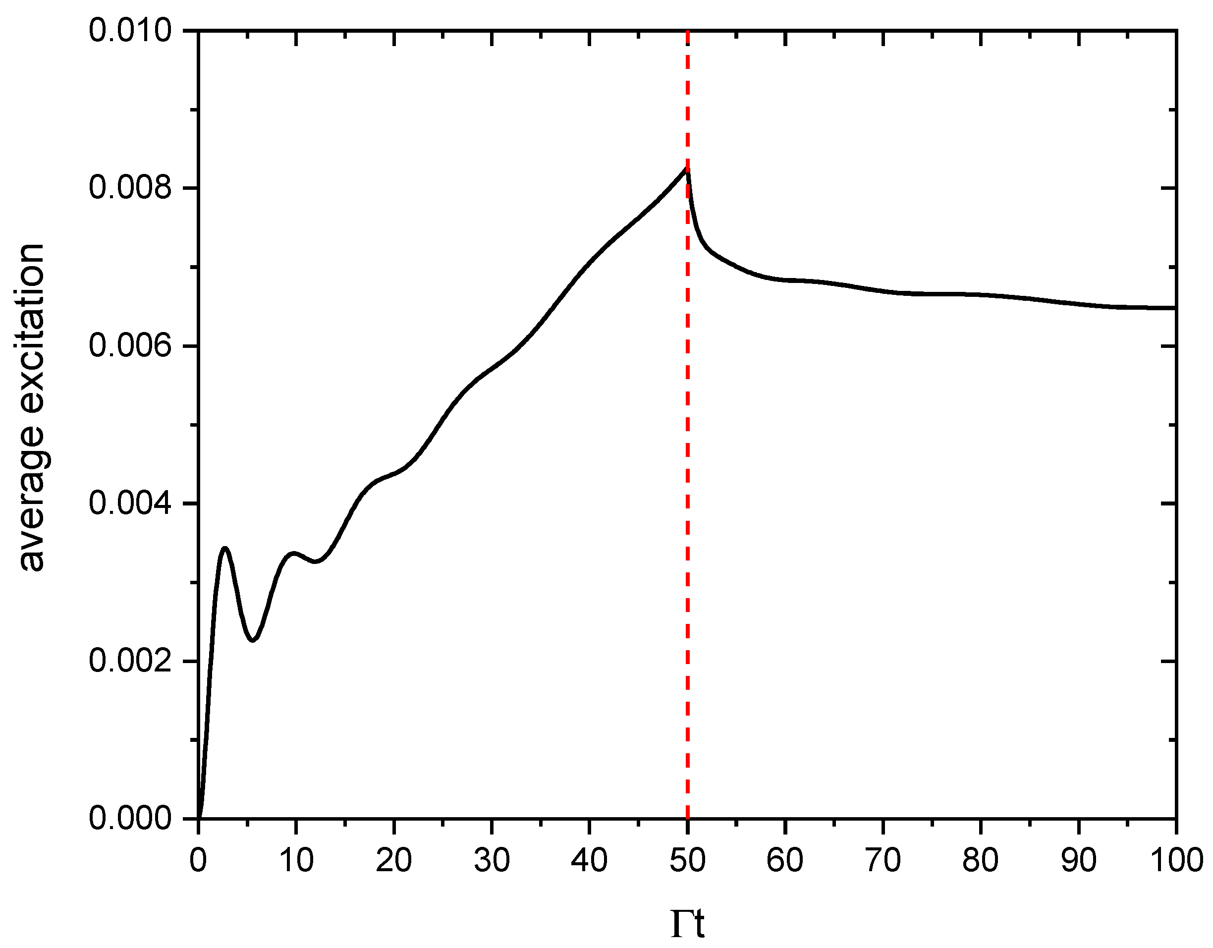
We now consider again the same chain of $N=100$ atoms with $a=\pi /2$, but driven by a resonant laser, with ${\Omega }_0=0.1$ and ${\Delta }_0=0$. The most interesting case is that of the scalar model, obtained by assuming $\delta =54.37°$ in the vectorial Equation (38); Figure 9 shows the average excitation, $⟨|\beta {|}^2⟩$ vs. $\Gamma t$, where the drive field is switched off at $\Gamma t=50$ (vertical dashed line). The average excitation grows almost linearly when the laser is turned on, typical for a diffusive regime [38,39]. After the laser is off, the excitation decays very slowly, showing that the excitation remains trapped in the atomic chain. We can understand this peculiar behavior by observing the probability density $P(x,t)$ in Figure 10 at $t=50/\Gamma$ (laser switch-off time, red line) and at $t=100/\Gamma$ (blue line). Contrarily to the detuned case, at resonance the subradiant region of the spectrum is already populated when the laser is on (red line of Figure 10). After the laser has been switched off, $P(x,t)$ remains almost the same, with only the radiating components, for $x<a$, decayed at $\Gamma t=100$ (blue line in Figure 10). Since now the spectrum is completely in the subradiant region $x>a$, the decay rate is almost zero and the atoms remain excited for a sufficiently long time.

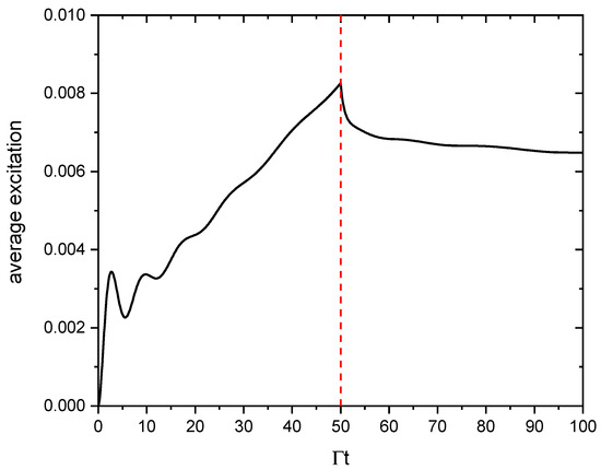
Figure 9. Average excitation, $⟨|\beta {|}^2⟩$, vs. $\Gamma t$ of a chain of $N=100$ with $a=\pi /2$, driven by a continuous resonant laser field, with ${\Omega }_0=0.1$ and ${\Delta }_0=0$, switched off at $\Gamma t=50$ (vertical dashed line).

Figure 10. $P(x,t)$ vs. x at $t=50/\Gamma$ (laser switch-off time, red line) and at $t=100/\Gamma$ (blue line), for $a=\pi /2$, $N=100$, ${\Omega }_0=0.1$, and ${\Delta }_0=0$. The dashed line is the value $x=a$.

5. Radiated Intensity

The following important question arises: May the probability $P(x,t)$ be determined by measuring the scattered intensity at a certain angle $\theta$ with respect to the chain’s axis? We know that the scattered field appears as a sum of wavelets radiated by the atomic dipoles, with the polarization component of the electric field

$$E_{\alpha }(\mathbf{r},t)={\displaystyle \frac{\hslash }{ie\mu }}\sum _{\beta }\sum _{j=1}^N{G}_{\alpha ,\beta }(k_0|\mathbf{r}-{\mathbf{r}}_j\left|\right){\beta }_j\left(t\right)$$

(45)

where $G_{\alpha ,\beta }\left(\mathbf{r}\right)$ is defined by Equation (25). In the far-field limit, one has $k_0|\mathbf{r}-{\mathbf{r}}_j|\approx k_{0}r-\mathbf{k}·{\mathbf{r}}_j$, where $\mathbf{k}=k_0(\sin \theta \cos \varphi ,\sin \theta \sin \varphi ,\cos \theta )$ and ${\mathbf{r}}_j=d(j-1){\widehat{\mathbf{e}}}_z$, so the field of Equation (45) radiated in a direction $\widehat{\mathbf{n}}$ reads

$$\mathbf{E}(\theta ,t)\approx {\displaystyle \frac{3\hslash \Gamma }{2e\mu }}\widehat{\mathbf{n}}\times (\widehat{\mathbf{n}}\times \widehat{\mathbf{e}}){\displaystyle \frac{e^{i{k}_{0}r}}{k_{0}r}}\sum _{j=1}^N{e}^{-i{k}_{0}d\cos \theta (j-1)}{\beta }_j\left(t\right)$$

(46)

where $\widehat{\mathbf{e}}$ is the unit polarization vector of the dipoles, and the scattered intensity is

$$I_s(\theta ,t)\propto {\left|\sum _{j=1}^N{e}^{-i{k}_{0}d\cos \theta (j-1)}{\beta }_j\left(t\right)\right|}^2\propto P(k_z,t)$$

(47)

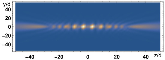
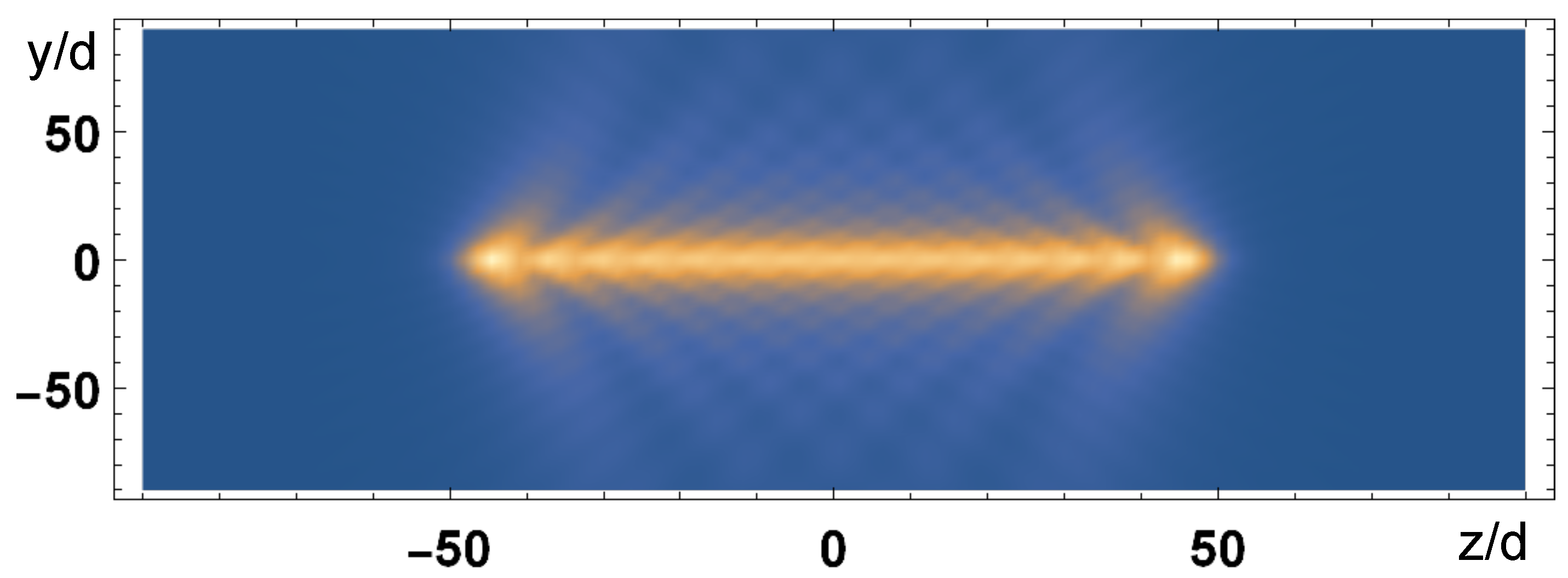
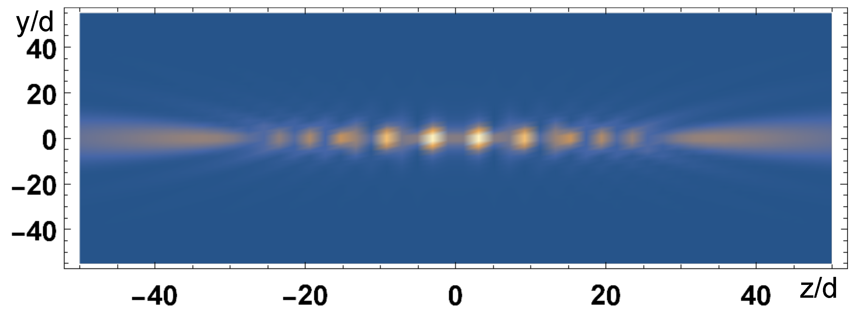
where $k_z=k_0\cos \theta$. Hence, the atoms radiate out of the chain’s axis for $|k_z|<k_0$. The subradiant region $|k_z|>k_0$ is not accessible by the scattered field, since it would be $\cos \theta >1$ and the electromagnetic field is evanescent in the directions transverse to the chain, since $k_{\perp }=i{k}_0\sqrt{{\cos }^2\theta -1}=i\xi$. Very few photons are emitted outside the chain’s axis direction (none in the case of an infinite chain). However, from the radiated intensity it is possible to see if the atomic state is subradiant or not, observing if the atoms are emitting in a direction out of the axis’ chain. This can be seen in Figure 11 and Figure 12, where we plot the field intensity $I_s\propto {\left|E_{\alpha }\right|}^2$ (where $E_{\alpha }$ is determined by Equation (45)) in the plane $x=5d$, emitted by a chain of $N=50$ atoms with $kd=1$, centered at $x=y=0$, for two different atomic distributions. Figure 11 shows a case of uniform excitation, with ${\beta }_j=1/\sqrt{N}$ such that $P\left(k_z\right)\propto N{\mathrm{sinc}}^2(k_{z}dN/2)$ and the probability distribution is peaked around $k_z=0$; in this case the atoms emit out of the chain’s axis. Figure 12 shows the emission from the most subradiant state, with ${\beta }_j$ given by Equation (43), such that $P\left(k_z\right)\approx 0$ for $k_z<k_0$; the field is evanescent and does not propagate out of the chain, remaining confined along the chain; since the chain is finite, most of the energy is radiated out at the ends of the chain [11].

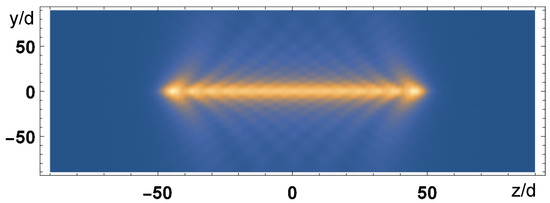
Figure 11. Field intensity (arb. units) in the plane $(y/d,z/d)$ at $x=5d$ emitted by a chain of $N=50$ atoms, with $kd=1$, along the z-axis, centered at $x=y=0$ and uniformly excited, ${\beta }_j=1/\sqrt{N}$. We observe that the field is radiated transversely to the chain.

Figure 12. Same as in Figure 11 but for the ${\beta }_j$ given by Equation (43), referred as the ‘most subradiant state’. We observe that the field is largely evanescent transverse to the chain, while most of the energy is radiated out at the ends of the chain.

6. Conclusions

In conclusion, we have discussed analytically and numerically how subradiance can emerge from the evolution of the dynamics of N two-level atoms in the single-excitation configuration along a linear chain. In the first part, we have characterized the spectrum of the decay rates and frequency shifts of the system, identifying the regions of the spectrum where spontaneous emission is enhanced or inhibited, up to a complete suppression in the case of an infinite chain. We proceeded first by obtaining a relation between the spectrum of emission and the single-particle amplitudes, whose evolution can be determined by solving the coupled-dipole equations. Then we have studied how different initial excitations evolve toward a subradiant state. A single-excited atom leads to an almost uniform population of subradiant modes. This suggested the idea that the atomic configuration leading to this uniform population can be calculated directly, obtaining what we named the ’most subradiant state’. Then, we investigated how subradiance may be induced by a driving laser, which excites the atoms and subsequently is switched off, such that the long-lived subradiant modes survive for a long time. Finally, we found the relation between spontaneous emitted intensity and subradiance. Subradiance is characterized by a suppression of the emission in the direction transverse to the chain axis. This analysis may be useful to envisage strategies to detect subradiance in ordered systems by measuring the radiation out of the lattice. The results obtained here for a linear chain can be extended to 2D and 3D lattices.

References

- Dicke, R.H. Coherence in spontaneous radiation processes. Phys. Rev. 1954, 93, 99. [Google Scholar] [CrossRef]
- Lehmberg, R.H. Radiation from an N-Atom system, I. General formalism. Phys. Rev. A 1970, 2, 883. [Google Scholar] [CrossRef]
- Bonifacio, R.; Schwendimann, P.; Haake, F. Quantum Statistical Theory of Superradiance I. Phys. Rev. A 1971, 4, 302. [Google Scholar] [CrossRef]
- Gross, M.; Haroche, S. Superradiance: An Essay on the Theory of Collective Spontaneous Emission. Phys. Rep. 1982, 93, 301. [Google Scholar] [CrossRef]
- Bienaimé, T.; Piovella, N.; Kaiser, R. Controlled Dicke subradiance from a large cloud of two-level systems. Phys. Rev. Lett. 2012, 108, 123602. [Google Scholar] [CrossRef]
- Guerin, W.; Araùjo, M.O.; Kaiser, R. Subradiance in a large cloud of cold atoms. Phys. Rev. Lett. 2016, 116, 083601. [Google Scholar] [CrossRef] [PubMed]
- Das, D.; Lemberger, B.; Yavuz, D.D. Subradiance and Superradiance-to-Subradiance Transition in Dilute Atomic Clouds. Phys. Rev. A 2020, 102, 043708. [Google Scholar] [CrossRef]
- Ferioli, G.; Glicenstein, A.; Henriet, L.; Ferrier-Barbut, I.; Browaeys, A. Storage and release of subradiant excitations in a dense atomic cloud. Phys. Rev. X 2021, 11, 021031. [Google Scholar] [CrossRef]
- Bettles, R.J.; Gardiner, S.A.; Adams, C.S. Cooperative eigenmodes and scattering in one-dimensional atomic arrays. Phys. Rev. A 2016, 94, 043844. [Google Scholar] [CrossRef]
- Facchinetti, G.; Jenkins, S.D.; Ruostekoski, J. Storing light with subradiant correlations in arrays of atoms. Phys. Rev. Lett. 2016, 117, 243601. [Google Scholar] [CrossRef]
- Asenjo-Garcia, A.; Moreno-Cardoner, M.; Albrecht, A.; Kimble, H.J.; Chang, D.E. Exponential improvement in photon storage fidelities using subradiance and “selective radiance” in atomic arrays. Phys. Rev. X 2017, 7, 031024. [Google Scholar] [CrossRef]
- Rui, J.; Wei, D.; Rubio-Abadal, A.; Hollerith, S.; Zeiher, J.; Stamper-Kurn, D.M.; Gross, C.; Bloch, I. A Subradiant Optical Mirror Formed by a Single Structured Atomic Layer. Nature 2020, 583, 369. [Google Scholar] [CrossRef]
- Cech, M.; Lesanovsky, I.; Olmos, B. Dispersionless subradiant photon storage in one-dimensional emitter chains. Phys. Rev. A 2023, 108, L051702. [Google Scholar] [CrossRef]
- Piovella, N. Cooperative Decay of an Ensemble of Atoms in a One-Dimensional Chain with a Single Excitation. Atoms 2024, 12, 43. [Google Scholar] [CrossRef]
- Bellando, L.; Gero, A.; Akkermans, E.; Kaiser, R. Cooperative effects and disorder: A scaling analysis of the spectrum of the effective atomic Hamiltonian. Phys. Rev. A 2014, 90, 063822. [Google Scholar] [CrossRef]
- Cottier, F.; Kaiser, R.; Bachelard, R. Role of disorder in super- and subradiance of cold atomic clouds. Phys. Rev. A 2018, 98, 013622. [Google Scholar] [CrossRef]
- Fofanov, Y.A.; Sokolov, I.M.; Kaiser, R.; Guerin, W. Subradiance in dilute ensembles: Role of pairs and multiple scattering. Phys. Rev. A 2021, 104, 023705. [Google Scholar] [CrossRef]
- Nienhuis, G.; Schuller, F. Spontaneous emission and light scattering by atomic lattice models. J. Phys. B Atom. Mol. Phys. 1987, 20, 23. [Google Scholar] [CrossRef]
- Zoubi, H.; Ritsch, H. Metastability and Directional Emission Characteristics of Excitons in 1D Optical Lattices. Europhys. Lett. 2010, 90, 23001. [Google Scholar] [CrossRef]
- Jenkins, S.D.; Ruostekoski, J. Controlled manipulation of light by cooperative response of atoms in an optical lattice. Phys. Rev. A 2012, 86, 031602. [Google Scholar] [CrossRef]
- Bettles, R.J.; Gardiner, S.A.; Adams, C.S. Cooperative Ordering in Lattices of Interacting Two-Level Dipoles. Phys. Rev. A 2015, 92, 063822. [Google Scholar] [CrossRef]
- Needham, J.A.; Lesanovsky, I.; Olmos, B. Subradiance-protected excitation transport. New J. Phys. 2019, 21, 073061. [Google Scholar] [CrossRef]
- Masson, S.J.; Ferrier-Barbut, I.; Orozco, L.A.; Browaeys, A.; Asenjo-Garcia, A. Many-Body Signature of Collective Decay in Atomic Chains. Phys. Rev. Lett. 2020, 125, 263601. [Google Scholar] [CrossRef] [PubMed]
- Masson, S.J.; Asenjo-Garcia, A. Universality od Dicke superradiance in arrays of quantum emitters. Nat. Commun. 2022, 13, 2285. [Google Scholar] [CrossRef] [PubMed]
- Ruostekoski, J. Cooperative quantum-optical planar arrays of atoms. Phys. Rev. A 2023, 108, 030101. [Google Scholar] [CrossRef]
- Jenkins, S.D.; Ruostekoski, J.; Papasimakis, N.; Savo, S.; Zheludev, N.I. Many-Body Subradiant Excitations in Metamaterial Arrays: Experiment and Theory. Phys. Rev. Lett. 2017, 119, 05390. [Google Scholar] [CrossRef] [PubMed]
- Solano, P.; Barberis-Blostein, P.; Fatemi, F.K.; Orozco, L.A.; Rolston, S.L. Super-radiance reveals infinite-range dipole interactions through a nanofiber. Nat. Commun. 2017, 8, 1857. [Google Scholar] [CrossRef]
- Jen, H.H.; Chang, M.-S.; Chen, Y.-C. Cooperative single photon subradiant states. Phys. Rev. A 2016, 94, 013803. [Google Scholar] [CrossRef]
- Holzinger, R.; Plankensteiner, D.; Ostermann, L.; Ritsch, H. Nanoscale Coherent Light Source. Phys. Rev. Lett. 2020, 124, 253603. [Google Scholar] [CrossRef]
- Sonnefraud, Y.; Verellen, N.; Sobhani, H.H.; Vandenbosch, G.A.E.; Moshchalkov, V.V.; Dorpe, P.V.; Nordlander, P.; Maier, S.A. Experimental realization of subradiant, superradiant, and Fano resonances in ring/disk plasmonic nanocavities. ACS Nano 2010, 4, 1664. [Google Scholar] [CrossRef]
- McGuyer, B.H.; McDonald, M.; Iwata, G.Z.; Tarallo, M.G.; Skomorowski, W.; Moszynski, R.; Zelevinsky, T. Precise study of asymptotic physics with subradiant ultracold molecules. Nat. Phys. 2015, 11, 32. [Google Scholar] [CrossRef]
- Morsch, O.; Oberthaler, M. Dynamics of Bose-Einstein condensates in optical lattices. Rev. Mod. Phys. 2006, 78, 179. [Google Scholar] [CrossRef]
- Hadzibabic, Z.; Stock, S.; Battelier, B.; Bretin, V.; Dalibard, J. Interference of an Array of Independent Bose-Einstein Condensates. Phys. Rev. Lett. 2004, 93, 180403. [Google Scholar] [CrossRef] [PubMed]
- Akkermans, E.; Gero, A.; Kaiser, R. Photon localization and Dicke superradiance in atomic gases. Phys. Rev. Lett. 2008, 101, 103602. [Google Scholar] [CrossRef] [PubMed]
- Bienaimé, T.; Bachelard, R.; Piovella, N.; Kaiser, R. Cooperativity in light scattering by cold atoms. Fortschritte Phys. 2013, 61, 377. [Google Scholar] [CrossRef]
- Scully, M.O.; Fry, E.; Ooi, C.H.R.; Wodkiewicz, K. Directed Spontaneous Emission from an Extended Ensemble of N Atoms: Timing Is Everything. Phys. Rev. Lett. 2006, 96, 010501. [Google Scholar] [CrossRef]
- Scully, M.O. Single photon subradiance: Quantum control of spontaneous emission and ultrafast readout. Phys. Rev. Lett. 2015, 115, 243602. [Google Scholar] [CrossRef]
- Holstein, T. Imprisonment of Resonance Radiation in Gases. Phys. Rev. 1947, 72, 1212. [Google Scholar] [CrossRef]
- Labeyrie, G.; Vaujour, E.; Müller, C.; Delande, C.; Miniatura, C.; Wilkowski, D.; Kaiser, R. Slow diffusion of light in a cold atomic cloud. Phys. Rev. Lett. 2003, 91, 223904. [Google Scholar] [CrossRef]
Disclaimer/Publisher’s Note: The statements, opinions and data contained in all publications are solely those of the individual author(s) and contributor(s) and not of MDPI and/or the editor(s). MDPI and/or the editor(s) disclaim responsibility for any injury to people or property resulting from any ideas, methods, instructions or products referred to in the content. |
© 2025 by the author. Licensee MDPI, Basel, Switzerland. This article is an open access article distributed under the terms and conditions of the Creative Commons Attribution (CC BY) license (https://creativecommons.org/licenses/by/4.0/).