Performance Tests and Improvements on the rmcdhf and rci Programs of GRASP

Abstract

The latest published version of GRASP (General-purpose Relativistic Atomic Structure Package), i.e., GRASP2018, retains a few suboptimal subroutines/algorithms, which reflect the limited memory and file storage of computers available in the 1980s. Here we show how the efficiency of the relativistic self-consistent-field (SCF) procedure of the multiconfiguration-Dirac–Hartree–Fock (MCDHF) method and the relativistic configuration-interaction (RCI) calculations can be improved significantly. Compared with the original GRASP codes, the present modified version reduces the CPU times by factors of a few tens or more. The MPI performances for all the original and modified codes are carefully analyzed. Except for diagonalization, all computational processes show good MPI scaling.

1. Introduction

Atomic energy levels, oscillator strengths, transition probabilities and energies are essential parameters for abundance analysis and diagnostics in astrophysics and plasma physics. In the past decade, the atomic spectroscopy group of Fudan University carried out two projects to calculate transition characteristics with high accuracy in collaboration with other groups. One project focused on the ions with $Z\lesssim 30$, which are generally of astrophysical interest, and the other on tungsten ions ($Z=74$), which are relevant in the research of magnetic confinement fusion. Employing the multiconfiguration Dirac–Hartree–Fock (MCDHF) approach [1,2,3,4,5], implemented within the GRASP2K package [6], and/or the relativistic many-body perturbation theory (RMBPT) [7], implemented within the FAC package [8,9,10], we performed a series of systematic and large-scale calculations of radiative atomic data for ions of low and medium Z-values belonging to the He I [11], Be I-Ne I [12,13,14,15,16,17,18,19,20,21,22], Si I-Cl I [23,24,25,26,27] isoelectronic sequences, and for the highly-charged isonuclear sequence ions of tungsten [28,29,30,31,32,33]. A large amount of atomic data, including level energies, transition wavelengths, line strengths, oscillator strengths, transition probabilities and lifetimes, were obtained. Their uncertainties were comprehensively assessed by cross-validations between the MCDHF and RMBPT results and by detailed comparisons with observations. It showed that spectroscopic accuracy was achieved for the computed excitation and transition energies in most of the ions concerned due to the fact that electron correlation was treated at a high level of approximation by using a very large expansion of configuration state functions (CSF) based on extended sets of one-electron orbitals. To make these large-scale calculations feasible and tractable, many efforts were devoted to improving the performance and stability of the codes used. Here, we describe some improvements made in the last two years for the rmcdhf and rci programs, which have not yet been included in the latest published version of GRASP, i.e., GRASP2018 [34].

The GRASP2018 package is an updated Fortran 95 version of recommended programs from GRASP2K Version 1_1 [6], providing improvements in accuracy and efficiency in addition to the translation from Fortran 77 to Fortran 95 [34]. However, it has retained some original subroutines/algorithms that reflect the limited memory and file storage capacities of computers in the 1980s, when the first versions of GRASP were released [2]. For example, the spin-angular coefficients, which are used to build the Hamiltonian matrix and the potentials, are stored on disks in unformatted files. During the iterations of the self-consistent-field (SCF) calculations, aiming to optimize the one-electron radial functions, the spin-angular coefficients are read from disks again and again. The calculations using expansions of hundreds of thousands of CSFs are very time-consuming, as the disk files easily exceed over 10 GB. This kind of inefficiency, which was considered a major bottleneck of the GRASP package for a long time, was removed very recently by one of the authors (GG) through two programs, rmcdhf_mem and rmcdhf_mem_mpi, which have been uploaded to the GRASP depository [35]. The new feature of these two programs is that the spin-angular coefficients, once they are read from disk files, are stored in memory by using arrays. In the present work, we show that these codes can be further improved by redesigning the procedure to obtain the direct and exchange potentials and the Lagrange multipliers, which are used to update the radial orbitals (large and small components) during the SCF procedure.

Once the radial functions have been determined by an MCDHF calculation based on the Dirac–Coulomb Hamiltonian, subsequent relativistic configuration-interaction (RCI) calculations are often performed to include the transverse photon interaction (which reduces to the Breit interaction at the low-frequency limit) and the leading quantum electrodynamics (QED) corrections. At this stage, the CSFs expansions are usually considerably enlarged to capture additional electron correlation effects. For example, our recent MCDHF calculations on C-like ions [16] were performed using an expansion of about two-million CSFs, which were generated by single and double (SD) excitations from the outer subshells of the multi-reference (MR) configurations, taking only the valence–valence correlation into account. The subsequent RCI calculations were based on approximately 20 million CSFs to adequately account for the additional core-valence (CV) electron correlation effects.

MCDHF and RCI calculations, using large CSFs expansions, require a lot of computing resources. Firstly, the construction of the Hamiltonian matrix is very time-consuming. The spin-angular integration of the Hamiltonian between pairs of CSFs has to be performed $N(N+1)/2$ times, where N is the order of the interaction matrix, i.e., the size of CSFs expansion for the block of given J and parity. Fortunately, we recently implemented a computational methodology based on configuration state function generators (CSFGs) that relaxes the above scaling. Instead of having to perform the spin-angular integration for each of the elements in the Hamiltonian matrix, the use of generators makes it possible to restrict the integration to a limited number of cases and then directly infer the spin-angular coefficient for all matrix elements between groups of CSFs spanned by the generators, which takes advantage of the fact that spin-angular expressions are independent of the principal quantum number [36]. Secondly, the time for solving the eigenvalue problem in MCDHF and RCI may also be significant, especially if many eigenpairs are required, as is normally the case in spectrum calculations for complex systems [16,23,24,25,26,27].

The present paper, which reports on improvements both for MCDHF and RCI, is organized as follows:

• In Section 2, we show how the diagonalization procedure in MCDHF and RCI calculations can be improved by further parallelization.
• In Section 3, we discuss the improvements in the MCDHF program resulting from the new management of spin-angular coefficients in memory and from the redesign of the procedures for calculating the potentials and Lagrange multipliers. Results are reported from a number of performance tests.
• In Section 4, we study the improvements in RCI performances thanks to the use of CSFGs. We also investigate the time ratios for constructing and diagonalizing the Hamiltonian matrix to determine the desired eigenpairs.
• Finally, in Section 5, we summarize the results of the performance tests and identify the remaining bottlenecks. This is followed by a discussion on how the latter could be circumvented in future developments.

2. Additional Parallelization for the DVDRC Library of GRASP

In the DVDRC library of GRASP, the Davidson algorithm [37], as implemented in [38], is used to extract the eigenpairs of interest from the interaction matrix. Assuming that the K lowest eigenpairs are required of a large, sparse, real and symmetric matrix $\mathit{A}$ of order N, the original Davidson algorithm can be described as shown in Algorithm 1, in which the upper limit of P, the order of the expanding basis, is defined by the variable $\mathrm{LIM}=2K+80$ in GRASP2018 [34]. The matrix-vector multiplication (6), which is the most time-consuming step, has already been parallelized in GRASP using message passing interface (MPI) by calling upon one of the three subroutines named DNICMV, SPODMV, and SPICMVMPI, depending on if the interaction matrix is sparse or dense, and stored in memory or on disk.

Algorithm 1: Davidson algorithm.

(0) Set $P=K$. Compute the initial Basis $\mathit{B}=\{{\mathit{b}}_1,\cdots ,{\mathit{b}}_P\}\in {\mathbb{R}}^{N\times P}$, $\mathit{D}=\mathit{AB}=\{{\mathit{d}}_1,\cdots ,{\mathit{d}}_P\}\in {\mathbb{R}}^{N\times P}$, and the projection $\mathit{S}={\mathit{B}}^T\mathit{AB}={\mathit{B}}^T\mathit{D}\in {\mathbb{R}}^{P\times P}$.     Repeat until converged steps (1) through (8):     (1) Solve the symmetric eigenvalue problem: $\mathit{SC}=\mathit{CU}$ (size $P\times P$).     (2) Target one of the K sought eigenpairs, say ($u,\mathit{c}$), $\mathit{c}\in {\mathbb{R}}^P$.     (3) If the basis size is maximal, restart: $\mathit{D}\leftarrow \mathit{DC}$, $\mathit{B}\leftarrow \mathit{BC}$, $\mathit{C}={\mathit{I}}_K$, $\mathit{S}=\mathit{U}$, $P=K$.     (4) Compute $\mathit{R}={(diag\left(\mathit{A}\right)-u\mathit{I})}^{-1}(\mathit{D}-u\mathit{B})\mathit{c}$.     (5) Orthogonalize: ${\mathit{b}}_{new}=\mathit{R}-\sum {\mathit{b}}_i{\mathit{b}}_i^T\mathit{R}$, normalize: ${\mathit{b}}_{new}\leftarrow {\mathit{b}}_{new}/\parallel {\mathit{b}}_{new}\parallel$.     (6) Matrix-vector multiplication: ${\mathit{d}}_{new}={\mathit{Ab}}_{new}$.     (7) Include ${\mathit{b}}_{new}$ in $\mathit{B}$ and ${\mathit{d}}_{new}$ in $\mathit{D}$. Increase P.     (8) Compute the new column of $\mathit{S}$: ${\mathit{S}}_{i,P}={\mathit{b}}_i^T{\mathit{d}}_P,i=1,\cdots ,P$.

It should be pointed out that the subroutines of the library in GRASP2018 [34] performing the remaining calculations, except for step (6) of the Davidson algorithm, are all serial. Step (1), solving the small symmetric eigenvalue problem of order P, which is generally smaller than 500, is very fast as it calls upon the DSPEVX routine from the LAPACK library. However, in steps (3)–(5) and (7)–(8), the matrix-vector, matrix–matrix multiplication and inner-products involve vectors of size N, such as all the column vectors of $\mathit{B}$ and $\mathit{D}$. In the MCDHF and RCI calculations, when N, the size of the CSFs expansion of a given J and parity, is large enough, and meanwhile, dozens of eigenpairs or more are searched, steps (3)–(5) and (7)–(8) can be as time-consuming as step (6). Hence, we have parallelized all the possibly time-consuming routines of the DVDRC library for these steps by using MPI, such as MULTBC, NRM_MGS, NEWVEC, ADDS, etc. We show in Section 3 and Section 4 that the CPU time for diagonalization can be significantly reduced by factors of about three in relatively large-scale calculations.

3. Improvements for MCDHF

3.1. Outline of the MCDHF Method

The theory of MCDHF has been comprehensively described in the literature; for examples, see [1,2,3,4,5]. Here it is outlined to explain the modifications of the original GRASP2018 codes. Atomic units are used throughout except for those given explicitly.

In MCDHF calculations with GRASP, only the Dirac–Coulomb Hamiltonian (${\mathcal{H}}_{\mathrm{D}\mathrm{C}}$) is taken into account. The Dirac one-electron orbital a is given by

$$u_a\left(\mathit{r}\right)=\frac{1}{r}\left(\begin{array}{c}{P}_{nlj}\left(r\right){\Omega }_{\kappa m}(\theta ,\varphi )\\ \mathrm{i}{Q}_{nlj}\left(r\right){\Omega }_{-\kappa m}(\theta ,\varphi )\end{array}\right),$$

(1)

in which P and Q are the radial functions, and $\Omega$ is the usual spherical spinor, i.e., the spin-angular function, $\kappa =-2(j-l)(j+1/2)$, $a\equiv (n,l,s,j,m)\equiv (n,\kappa ,m)$. For a state $\alpha$ of given total angular momentum J, total magnetic quantum number $M_J$, and parity $\pi$, the atomic state function (ASF) is formed by a linear combination of CSFs

$$\Psi \left(\alpha J{M}_J\pi \right)\equiv |\alpha J{M}_J\pi ⟩=\sum _{r=1}^{N_{CSF}}{c}_{\alpha ;r}\Phi \left({\gamma }_{r}J{M}_J\pi \right).$$

(2)

$N_{CSF}$ is the number of CSFs used in the expansion. Each CSF, $\Phi \left({\gamma }_{r}J{M}_J\pi \right)$, is constructed on four-component spinor orbital functions (1). The label ${\gamma }_r$ contains all the needed information on its structure, i.e., the constituent subshells with their symmetry labels and the way their angular momenta are coupled to each other in $jj$-coupling. The level energy $E_{\alpha }$ and the vector of expansion coefficients ${\mathit{c}}_{\alpha }$ are solved from the following secular equation:

$$(\mathit{H}-E_{\alpha }\mathit{I}){\mathit{c}}_{\alpha }=\mathbf{0},$$

(3)

with

$$E_{\alpha }=⟨\alpha J{M}_J\pi |{\mathcal{H}}_{\mathrm{D}\mathrm{C}}|\alpha J{M}_J\pi ⟩=\frac{1}{\sqrt{2J+1}}⟨\alpha J\pi \parallel {\mathcal{H}}_{\mathrm{D}\mathrm{C}}\parallel \alpha J\pi ⟩$$

(4)

where the reduced matrix element (RME) $⟨\alpha J\pi \parallel {\mathcal{H}}_{\mathrm{D}\mathrm{C}}\parallel \alpha J\pi ⟩$ is defined from Edmond’s formulation of the Wigner–Eckart theorem [39]. This RME can be developed in terms of RMEs in the CSF basis, $H_{rs}=⟨{\Phi }_r\left({\gamma }_{r}J\right)\parallel {\mathcal{H}}_{\mathrm{D}\mathrm{C}}\parallel {\Phi }_s\left({\gamma }_{s}J\right)⟩$, which are generally expressed as

$$H_{rs}=\sum _{ab}{t}_{ab}^{rs}I(a,b)+\sum _{abcdk}{v}_{abcd;k}^{rs}{R}^k(ab,cd).$$

(5)

The radial integrals $I(a,b)$ and $R^k(ab,cd)$ are, respectively, relativistic kinetic-energy and Slater integrals, $t_{ab}^{rs}$ and $v_{abcd;k}^{rs}$ are the corresponding spin-angular coefficients, and k is the tensor rank.

The radial functions of the orbitals are unknown and should be determined on a grid. The stationary condition with respect to variations in the radial functions, in turn, gives the following MCDHF integro-differential equations for each orbital a [1,2,3,4]:

$$\left\{\begin{array}{c}\hfill \left(\frac{d}{dr}+\frac{{\kappa }_a}{r}\right)P_a-\left(2c-\frac{{ϵ}_a}{c}-\frac{V_{\mathrm{nuc}}}{c}+\frac{Y_a}{cr}\right)Q_a=-\frac{1}{c{\overline{q}}_a}\sum _{b\ne a}^{n_w}{\delta }_{{\kappa }_a{\kappa }_b}{ϵ}_{ab}{Q}_b-\frac{X_a^{\left(P\right)}}{r},\\ \hfill \left(\frac{d}{dr}-\frac{{\kappa }_a}{r}\right)Q_a+\left(-\frac{{ϵ}_a}{c}-\frac{V_{\mathrm{nuc}}}{c}+\frac{Y_a}{cr}\right)P_a=\frac{1}{c{\overline{q}}_a}\sum _{b\ne a}^{n_w}{\delta }_{{\kappa }_a{\kappa }_b}{ϵ}_{ab}{P}_b+\frac{X_a^{\left(Q\right)}}{r},\end{array}\right.$$

(6)

in which the Lagrange multipliers ${ϵ}_a$ and ${ϵ}_{ab}$ ensure that the $n_w$ orbitals of $\{a,b,\cdots \}$ form an orthonormal set. The direct potential $Y_a\left(r\right)$ arising from the two-body interactions, summing over the allowed tensor rank k, is given by

$$Y_a\left(r\right)=-\sum _{b=1}^{n_w}\sum _k{y}^k\left(ab\right)Y^k(bb;r)-\sum _k\sum _{b,d}{y}^k\left(abad\right)Y^k(bd;r),$$

(7)

with $Y^k(;r)$ being the relativistic one-dimensional radial integrals [1,2,3,4], and

$$\overline{q}\left(a\right)y^k\left(ab\right)/(1+{\delta }_{ab})=\sum _r{d}_{rr}{f}_r^k\left(ab\right),$$

(8)

$$\overline{q}\left(a\right)y^k\left(abad\right)=\sum _{r,s}{d}_{rs}{v}_{abad;k}^{rs},$$

(9)

where $f_r^k\left(ab\right)\equiv v_{abab;k}^{rr}$ and $v_{abad;k}^{rs}$ are the spin-angular coefficients. The exchange potentials $X_a\left(r\right)$ in Equation (6) are given by

$$\begin{array}{cc}\hfill & X_a^{\left(P\right)}\left(r\right)=\frac{1}{c}\left[\sum _{b\ne a}^{n_w}\sum _k{x}^k\left(ab\right)Y^k(ab;r)Q_b+\sum _{bcd,c\ne a}\sum _k{x}^k\left(abcd\right)Y^k(bd;r)Q_c\right],\hfill \\ \hfill & X_a^{\left(Q\right)}\left(r\right)=\frac{1}{c}\left[\sum _{b\ne a}^{n_w}\sum _k{x}^k\left(ab\right)Y^k(ab;r)P_b+\sum _{bcd,c\ne a}\sum _k{x}^k\left(abcd\right)Y^k(bd;r)P_c\right],\hfill \end{array}$$

(10)

with

$$\overline{q}\left(a\right)x^k\left(ab\right)=\sum _r{d}_{rr}{g}_r^k\left(ab\right),$$

(11)

$$\overline{q}\left(a\right)x^k\left(abcd\right)=\sum _{rs}{d}_{rs}{v}_{abcd;k}^{rs},$$

(12)

where $g_r^k\left(ab\right)\equiv v_{abba;k}^{rr}$ and $v_{abcd;k}^{rs}$ are also the spin-angular coefficients. The coefficients $d_{rs}$ are the generalized weights

$$d_{rs}=\sum _{\alpha =1}^{n_L}{g}_{\alpha }{c}_{\alpha ;r}{c}_{\alpha ;s}$$

(13)

in which $g_{\alpha }$ is the weight attributed to level $\alpha$, and $n_L$ is the number of targeted levels. In the extended optimal level (EOL) calculation of GRASP, the MCDHF optimization procedure ensures that the average energy weighted by $g_{\alpha }$, i.e., $\overline{E}=\sum g_{\alpha }{E}_{\alpha }$, is stationary with respect to small changes of the orbitals and expansion mixing coefficients. In all of the above equations, $\overline{q}\left(a\right)$ is the generalized occupation number of orbital a:

$$\overline{q}\left(a\right)=\sum _r{d}_{rr}{q}_r\left(a\right),$$

(14)

where $q_r\left(a\right)$ is the occupation number for orbital a of CSF r. The resulting direct and exchange potentials are also used to determine the Lagrange multipliers [1].

It should be mentioned that $b,c,d\ne a$ is assumed in both Equations (9) and (12), whose left-hand sides should be multiplied by some adequate factors if $b=a$ and/or $d=a$, as given in Equation (8). In addition, the contributions to the exchange potential arising from off-diagonal one-body integrals $I(a,b)$${\delta }_{{\kappa }_a,{\kappa }_b}$ are not presented here, but they have been included since the GRASP92 version [40].

Spin-angular coefficients $f_r^k\left(ab\right)$ and $g_r^k\left(ab\right)$ are known in closed forms [1,2] and calculated during the constructions of potentials and the Hamiltonian matrix, whereas $v_{abcd;k}^{rs}$, as well as $t_{ab}^{rs}$ involving a one-body integral $I(a,b)$, are obtained from the unformatted disk files, namely mcp.XXX, which are generated by the rangular program [41,42,43] of GRASP.

3.2. Redesigning the Calculations of Potentials

The MCDHF calculations are generally divided into two parts, i.e., (i) searching the concerned eigenpairs from solving Equation (3) for a given set of one-electron orbitals and (ii) updating the orbitals from iteratively solving the orbital equations Equation (6) for a given set of mixing coefficients. In addition to the additional parallelization for the DVDRC Library of GRASP mentioned in Section 2, the computational task can be reduced significantly by redesigning the calculations of potentials.

The general MCDHF procedure used in rmcdhf or rmcdhf_mpi programs of GRASP2018 [34] is illustrated in Algorithm 2. The notes integrated in the description of the SCF procedure outline the modifications provided in the memory-version rmcdhf_mem and rmcdhf_mem_mpi [35], and the present modified version referred to as rmcdhf_mpi_FD for convenience. Only the parallel versions are referred to hereinafter, as we focus on large-scale MCDHF calculations.

Algorithm 2: SCF procedure.

(0.0) Load all of the mcp.XXX files into arrays. Note: This step is added in both rmcdhf_mem_mpi and rmcdhf_mpi_FD.     (0.1) Initialize the orbitals, read CSFs expansion, perform any other needed initialization.     (0.2) Determine NEC, the number (NEC) of needed off-diagonal Lagrange multipliers ${ϵ}_{ab}$ with $a\ne b$ and ${\kappa }_a={\kappa }_b$, and subshells a and/or b are partially occupied. Labels a and b recorded.     (0.3) Call MATRIXmpi and then MANEIGmpi, set H-matrix and solve Equation (6) to obtain $E_{\alpha }^{\left(0\right)}$ and ${\mathit{c}}_{\alpha }^{\left(0\right)}$, $\alpha =1,\cdots ,n_L$, calculate ${\overline{q}}^{\left(0\right)}$ for all orbitals and ${\overline{E}}^{\left(0\right)}$. Note: Additional parallelizations for the DVDRC library presented in Section 2 are included in rmcdhf_mpi_FD.     (0.4) For each orbital a involved in the NEC off-diagonal Lagrange multipliers, construct the sorted NYA and NXA arrays storing the unique and packed labels to identify the possible direct and exchange contributions in Equations (7) and (10), respectively. Note: This step is added in rmcdhf_mpi_FD.     Start the SCF procedure, repeat until $\overline{E}$ converged, in the ith loop:     (1.0) For all orbitals a involved in the calculations of NEC off-diagonal Lagrange multipliers, update the $y^k$ and $x^k$ coefficients needed in Equations (7) and (10), respectively, by using Equations (8) and (9) or by Equations (11) and (12) in which ${\overline{q}}^{(i-1)}$ is used. The eigenvector matrix ${\mathit{c}}^{(i-1)}$ is used in Equation (13). The results are saved in YA and XA arrays in the same order of NYA and NXA arrays. Note: This step is added in rmcdhf_mpi_FD.     (1.1) Call routine SetLAGmpi to determine the needed NEC off-diagonal Lagrange multipliers ${ϵ}_{ab}$              (a1) For orbital a, call routine SETCOF to build unsorted NYA and NXA arrays, sequentially update the needed $y^k$ and $x^k$ coefficients. Note: This step is removed in rmcdhf_mpi_FD as the needed data have been obtained in steps (0.4) and (1.0).              (a2) Build the potentials for orbital a by calling routines YPOT, XPOT and DACON. Note: Routines YPOT and XPOT have been parallelized using MPI in rmcdhf_mpi_FD.              (b1) As done in (a1) but for orbital b. Note: This step is removed in rmcdhf_mpi_FD.              (b2) As done in (a2) but for orbital b.              (c1) Calculate ${ϵ}_{ab}$ from the equations given in [1].     (2) Call routine IMPROVmpi to update the orbitals by solving Equation (6), update the potentials for each varied orbital by calls of SETCOF, YPOT, XPOT, etc. Note: The inside calling routine SETCOF is removed in rmcdhf_mpi_FD.     (3) As done in step (0.3) but using the updated orbitals, obtain $E_{\alpha }^{\left(i\right)}$, ${\mathit{c}}_{\alpha }^{\left(i\right)}$, ${\overline{E}}^{\left(i\right)}$ and ${\overline{q}}^{\left(i\right)}$, etc.

We describe some of the modifications in detail below:

• One routine SETMCP_MEM is added in rmcdhf_mem_mpi and retained in rmcdhf_mpi_FD to read the $t_{ab}^{rs}$ and $v_{abcd;k}^{rs}$ spin-angular coefficients together with the corresponding packed orbital labels from mcp.XXX disk-files into arrays. When needed, the data are fetched from memory in rmcdhf_mem_mpi and rmcdhf_mpi_FD, whereas rmcdhf_mpi reads the mcp.XXX disk-files in steps (0.3), (a1), (b1), (2) and (3) of Algorithm 2.
• The most time-consuming SETCOF subroutine of rmcdhf_mpi is split into two routines, i.e., SETTVCOF and SETALLCOF in rmcdhf_mpi_FD.

  -

  During the first call just before the SCF iterations start, SETTVCOF records the Slater integrals $R^k(ab,cd)$ contributing to the NEC off-diagonal Lagrange multipliers, the packed labels, i.e., $LABV=\left(\right(IA\times KEY+IB)\times KEY+IC)\times KEY+ID$ with $KEY=215$ (and $n_w\le 214$, which is the maximum value allowing for that LABV variable that may be stored as an integer of 4 bytes), and the corresponding tensor rank k are saved into arrays. $IA,IB,IC,ID$ are, respectively, the positions of $a,b,c,d$ in the set consisting of $n_w$ orbitals. There are many identical Slater integrals $R^k(ab,cd)$ arising from different $J^{\pi }$ blocks.

  -

  During the SCF procedure, SETTVCOF only performs all the summations of Equations (9) and (12) within one entrance for each iteration.

  -

  Within the first entrance just before the SCF iterations start, SETALLCOF constructs the $NYA(:,a)$ and $NXA(:,a)$ arrays for all the orbitals involved in the calculations of all off-diagonal Lagrange multipliers. The diagonal Slater integrals $R^k(ab,ab)$ or $R^k(ab,ba)$ of the Hamiltonian matrix involved in the calculations for $y^k$ and $x^k$ (see Equations (8) and (11)), and those $R^k(ab,cd)$, recorded by SETTVCOF and involved in Equations (9) and (12), are considered. The labels $LABYk$ ($=(IB\times KEY+ID)\times KEY+k$) and $LABXk$ packed by $\left(\right((IC\times KEY+IB)\times KEY+ID)\times KEY)+k$ are sorted and saved into $NYA(:,a)$ and $NXA(:,a)$ arrays, respectively. Hence, $NYA(:,a)$ and $NXA(:,a)$ are sorted lists with distinct elements. All MPI processes are modified to have the same $NYA$ and $NXA$ arrays. The $y^k$ and $x^k$ coefficients, arising from the same Slater integrals but from different $J^{\pi }$ blocks, are accumulated, respectively, according to the $LABYk$ and $LABXk$ values stored in $NYA(:,a)$ and $NXA(:,a)$.

  -

  During SCF iterations, SETALLCOF only accumulates all the needed coefficients in Equations (7) and (10) across different $J^{\pi }$ blocks, employing a binary search strategy (with time complexity of $O(lo{g}_2\left(n\right)$) to match the $LABYk$ and $LABXk$ values with those stored in the $NYA$ and $NXA$ arrays, respectively. The accumulated $y^k$ and $x^k$ coefficients are saved into YA and XA arrays at the same positions as those of $LABYk$ and $LABXk$ in $NYA$ and $NXA$ arrays. This accumulation scheme significantly reduces the computation efforts for the relativistic one-dimensional radial integrals $Y^k(;r)$ in Equations (7) and (10).

  -

  In both SETTVCOF and SETALLCOF routines, the computation efforts are significantly reduced by taking advantage of the symmetry properties of Equations (8), (9), (11) and (12). Their right-hand sides, i.e., the summations, are the same for all the involved orbitals and performed only once within the individual SCF loop. For example, given $a\ne b\ne c\ne d$, the corresponding $R^k(ab,cd)$ contributes to the exchange parts of the four orbitals, and the associated four $x^k$ coefficients can be obtained simultaneously by considering their generalized occupation number.

  -

  In the SETCOF routine of rmcdhf_mpi, the symmetry properties are not yet considered. The $NYA$ and $NXA$ arrays are constructed again and again in each entrance and have repetitious labels for which the sequential search method (with time complexity of $O\left(n\right)$), used to accumulate the corresponding $y^k$ and $x^k$ coefficients, is inefficient. In MCDHF calculations using many orbitals, the number of labels $LABXk$ can easily exceed hundreds of thousands or even more. This inefficiency of rmcdhf_mpi significantly slows down the computations.

• In rmcdhf_mpi_FD, the subroutines YPOT and XPOT are parallelized by using MPI, whereas they are serial in both rmcdhf_mpi and rmcdhf_mem_mpi.
• Obviously, compared with rmcdhf_mpi and rmcdhf_mem_mpi, the new code rmcdhf_mpi_FD is more memory-consuming since many additional arrays possibly of large size are maintained during the SCF procedure, and dozens of additional GB of memory are needed if the number of labels $LABXk$ reaches several million.

3.3. Performance Tests for MCDHF

In the present section, we would like to compare the relative performances of the three available codes, rmcdhf_mpi, rmcdhf_mem_mpi and rmcdhf_mpi_FD, to perform MCDHF calculations. Here we choose two examples, i.e., Mg VII and Be I, to illustrate and discuss the improvements in efficiency obtained with the two new codes, i.e., rmcdhf_mem_mpi and rmcdhf_mpi_FD. The calculations are all performed using the Linux server with two Intel(R) Xeon(R) Gold 6 278C CPU (2.60 GHz) and 52 cores, except in some cases for which the used CPU is explicitly given. In this comparative work, we carefully checked that the results obtained with the three codes were identical. Throughout the present work, the reported CPU times are all wall-clock times, as they are more meaningful for the end-users.

3.3.1. Mg VII

In our recent work on C-like ions [16], large-scale MCDHF-RCI calculations were performed for the $n\le 5$ states in C-like ions from O III to Mg VII. Electron correlation effects were accounted for by using large configuration state function expansions, built from the orbital sets with principal quantum numbers $n\le 10$. A consistent atomic data set including both energies and transition data with spectroscopic accuracy was produced for the lowest hundreds of states of C-like ions from O III to Mg VII. Here we take Mg VII as an example to investigate the performances of rmcdhf_mpi, rmcdhf_mem_mpi and rmcdhf_mpi_FD programs.

In the MCDHF calculations of [16] aiming at the orbital optimisation, the CSF expansions were generated by SD-excitations up to $10\left(spdfghi\right)$ orbitals from all possible $\left(1s^2\right)2l^3{n}^{\prime }{l}^{\prime }$ with $2\le n^{\prime }\le 5$ configurations. (More details can be found in [16].) The MCDHF calculations were performed layer by layer using the following sequence of active sets (AS):

$$\begin{array}{cc}\hfill A{S}_1& =\{6s,6p,6d,6f,6g,6h\},\hfill \\ \hfill A{S}_2& =\{7s,7p,7d,7f,7g,7h,7i\},\hfill \\ \hfill A{S}_3& =\{8s,8p,8d,8f,8g,8h,8i\},\hfill \\ \hfill A{S}_4& =\{9s,9p,9d,9f,9g,9h,9i\},\hfill \\ \hfill A{S}_5& =\{10s,10p,10d,10f,10g,10h,10i\}.\hfill \end{array}$$

Here the test calculations are carried out only for the even states with J = 0–3. The CSF expansions using the above AS orbitals, as well as the number of targeted levels for each block, are listed in Table 1. To keep the calculations tractable, only two SCF iterations are performed, taking the converged radial functions from [16] as the initial estimation. The zero- and first-order partition techniques [4,44], often referred to as ‘Zero-First’ methods [45], are employed. The zero-space contains the CSFs with orbitals up to $5\left(spdfg\right)$, the numbers of which are also reported in Table 1. The corresponding sizes of mcp.XXX files are, respectively, about 5.2, 11, 19, 29, and 41 GB in the $A{S}_1$ through $A{S}_5$ calculations.

Table 1. MCDHF calculations for the even states of Mg VII. For each J-block, the number of targeted levels (eigenpairs) and sizes (number of CSFs) of the zero-space and CSF-expansions for the different orbital active sets are listed.

	J = 0	J = 1	J = 2	J = 3
Eigenvalues	23	47	54	36
Zero space	3 931	11 060	15 487	16 089
AS1	9 912	31 046	45 779	49 053
AS2	19 449	65 099	99 824	109 618
AS3	32 534	113 193	177 519	197 601
AS4	49 167	175 328	278 864	313 002
AS5	69 348	251 504	403 859	455 821

The CPU times for these MCDHF calculations using the $A{S}_3$ and $A{S}_5$ orbital sets are reported in Table 2 and Table 3, respectively. To show the MPI performance, the calculations are carried out using various numbers of MPI processes (np) ranging from 1 to 48. The rmcdhf_mpi and rmcdhf_mem_mpi MPI calculations using the $A{S}_5$ orbitals set are only performed with $np\ge 8$, as the calculations with smaller $np$-values are too time-consuming. The CPU times are presented in the time sequence of Algorithm 2. For MCDHF calculations limited to two iterations, the eigenpairs are searched three times, i.e., once at step (0.3) and twice at step (3). The three rows with label “SetH&Diag” in Table 2 and Table 3 report the corresponding CPU times for setting the Hamiltonian matrix (routine MATRIXmpi) and for its diagonalization (routine MANEIGmpi), whereas the row with “Sum(SetH&Diag)” reports their sum. Steps (1.1) and (2) of Algorithm 2 are carried out twice in all calculations, as well as step (1.0) in rmcdhf_mpi_FD calculations. The rows labeled by “SetCof + LAG” and “IMPROV” report, respectively, the CPU times for routines SETLAGmpi and IMPROVmpi, i.e., for steps (1.1) and (2) of Algorithm 2, while the row “Update” gives their sum. The rows labeled “Sum(Update)” display the total CPU times needed to update the orbitals twice. The rows “Walltime” represent the total code execution times. The differences between the summed value “Sum(Update)” + “Sum(SetH&Diag)” and the “Walltime” ones represent the CPU times that are not monitored by the former two. It can be seen that these differences are relatively small in cases of rmcdhf_mpi and rmcdhf_mem_mpi, implying that most of the time-consuming parts of the codes have been included in the tables, while the relatively large differences in the case of rmcdhf_mpi_FD could be reduced if the CPU times needed for constructing the sorted NXA and NYA arrays in step (0.4) of Algorithm 2 would be taken into account.

Table 2. CPU times (in s) for the Mg VII AS₃ SCF calculations using the rmcdhf_mpi, rmcdhf_mem_mpi and rmcdhf_mpi_FD codes as a function of the number of MPI processes ($np$). See text for the label meanings.

np	1	2	4	8	16	24	32	40	48
					rmcdhf_mpi
SetH&Diag	1 001.71	752.79	608.58	565.55	522.02	546.13	576.30	648.67	759.93
					Iteration 1
SetCof + LAG	8 366.72	4 960.48	2 614.34	1 604.33	815.48	571.63	449.01	378.51	320.42
IMPROV	1 727.39	947.32	541.60	332.96	167.40	116.33	90.86	76.15	63.73
Update	10 094.10	5 907.80	3 155.94	1 937.29	982.89	687.96	539.88	454.66	384.15
SetH&Diag	165.64	88.89	50.55	35.02	24.23	18.59	21.29	21.08	21.49
					Iteration 2
SetCof + LAG	8 291.35	4 965.60	2 615.25	1 603.00	815.35	571.02	448.73	378.33	320.51
IMPROV	1 707.80	944.99	540.88	332.16	167.28	116.17	90.84	76.11	63.65
Update	9 999.14	5 910.59	3 156.13	1 935.16	982.63	687.18	539.57	454.45	384.15
SetH&Diag	167.34	83.26	47.78	29.61	22.60	19.88	18.23	21.88	18.68
Sum(SetH&Diag)	1 334.69	924.94	706.91	630.18	568.85	584.60	615.82	691.63	800.10
Sum(Update)	20 093.24	11 818.39	6 312.07	3 872.45	1 965.52	1 375.14	1 079.45	909.11	768.30
Walltime	21 467	12 773	7 044	4 528	2 554	1 978	1 714	1 619	1 587
					rmcdhf_mem_mpi
SetH&Diag	983.97	723.53	600.12	559.52	515.09	544.02	570.96	649.47	760.98
					Iteration 1
SetCof + LAG	3 152.54	1 858.49	1 205.67	833.63	454.55	312.74	252.01	214.02	170.87
IMPROV	644.27	381.98	246.99	171.34	91.89	62.32	49.69	41.80	33.40
Update	3 796.81	2 240.47	1 452.66	1 004.96	546.44	375.06	301.69	255.82	204.27
SetH&Diag	118.09	64.93	38.78	28.84	21.23	16.26	19.59	18.80	20.19
					Iteration 2
SetCof + LAG	3 028.23	1 859.01	1 205.41	833.44	454.53	312.95	251.81	214.09	171.05
IMPROV	616.07	381.84	246.87	171.41	91.94	62.29	49.69	41.79	33.39
Update	3 644.30	2 240.85	1 452.28	1 004.85	546.47	375.24	301.50	255.89	204.44
SetH&Diag	116.69	59.44	35.83	23.42	19.38	17.62	16.54	19.51	17.40
Sum(SetH&Diag)	1 218.75	847.90	674.73	611.78	555.70	577.90	607.09	687.78	798.57
Sum(Update)	7441.11	4 481.32	2 904.94	2 009.81	1 092.91	750.30	603.19	511.71	408.71
Walltime	8 822	5 420	3 636	2 662	1 677	1 353	1 233	1 221	1 228
					rmcdhf_mpi_FD
SetH&Diag	962.78	548.74	342.01	246.59	202.29	210.55	222.01	259.01	296.04
NXA&NYA	33.62	17.15	9.22	5.11	2.90	2.09	1.89	1.78	1.80
					Iteration 1
SetTVCof	130.05	68.21	38.31	23.73	11.84	7.96	6.18	5.09	4.39
WithoutMCP	125.65	32.55	12.06	6.72	3.07	2.08	1.26	1.02	0.80
WithMCP	0.41	0.41	0.40	0.41	0.43	0.42	0.42	0.42	0.43
SetLAG	4.61	2.33	4.06	0.64	0.69	0.47	0.53	0.33	0.24
SetCof + LAG	261.89	104.06	55.15	31.68	16.12	10.99	8.44	6.92	5.90
IMPROV	0.63	0.32	0.17	0.09	0.05	0.04	0.03	0.03	0.03
Update	262.52	104.38	55.32	31.77	16.16	11.03	8.47	6.94	5.93
SetH&Diag	118.26	67.76	37.13	25.90	18.96	15.28	13.52	17.35	20.45
					Iteration 2
SetTVCof	130.01	68.20	38.34	23.67	11.82	7.95	6.16	5.06	4.35
WithoutMCP	125.13	32.73	12.06	6.72	3.06	2.08	1.25	1.01	0.79
WithMCP	0.41	0.41	0.40	0.41	0.43	0.42	0.42	0.42	0.43
SetLAG	4.61	2.33	4.00	0.84	0.67	0.44	0.51	0.33	0.27
SetCof + LAG	261.28	104.23	55.11	31.83	16.08	10.95	8.39	6.86	5.88
IMPROV	0.63	0.32	0.17	0.09	0.05	0.04	0.03	0.03	0.03
Update	261.91	104.55	55.28	31.92	16.12	10.98	8.42	6.88	5.91
SetH&Diag	112.99	63.32	35.53	22.23	16.77	14.37	15.57	16.98	17.19
Sum(SetH&Diag)	1 194.03	679.82	414.67	294.72	238.02	240.20	251.10	293.34	333.68
Sum(Update)	524.43	208.93	110.60	63.69	32.28	22.01	16.89	13.82	11.84
Walltime	1 915	997	591	404	301	289	292	331	369

Table 3. CPU times (in s) for the Mg VII AS₅ SCF calculations using the rmcdhf_mpi, rmcdhf_mem_mpi and rmcdhf_mpi_FD codes as a function of the number of MPI processes ($np$). See text for the label meanings.

	rmcdhf_mpi			rmcdhf_mem_mpi			rmcdhf_mpi_FD
np	16	32	48	16	32	48	16	32	48
SetH&Diag	1 299.62	1 605.74	2 478.68	1 290.83	1 598.93	2 475.46	452.67	595.13	944.78
NXA&NYA							6.52	4.51	4.26
					Iteration 1
SetTVCof							28.25	13.82	9.90
WithoutMCP							22.14	9.55	7.15
WithMCP							1.19	1.19	1.13
SetLAG							10.32	3.38	1.79
SetCof + LAG	3 172.04	1 575.54	1 209.01	1 999.94	986.68	761.89	62.09	28.06	20.07
IMPROV	461.45	222.55	168.86	288.38	135.88	103.19	0.07	0.04	0.04
Update	3 633.49	1 798.09	1 377.87	2 288.32	1 122.56	865.08	62.16	28.10	20.11
SetH&Diag	54.67	59.44	55.03	47.39	55.00	51.87	58.24	41.64	48.01
					Iteration 2
SetTVCof							28.09	13.80	9.82
WithoutMCP							25.32	9.76	7.09
WithMCP							1.09	1.18	1.14
SetLAG							7.59	3.18	1.83
SetCof + LAG	3 174.72	1 576.07	1 207.94	2 000.64	986.54	761.64	62.27	28.02	19.95
IMPROV	461.71	222.33	168.74	288.50	135.88	103.11	0.07	0.04	0.04
Update	3 636.44	1 798.41	1 376.68	2 289.14	1 122.43	864.75	62.34	28.06	19.99
SetH&Diag	54.00	40.46	59.74	46.67	38.17	56.65	43.45	32.79	40.38
Sum(SetH&Diag)	1 408.29	1 705.64	2 593.45	1 384.89	1 692.10	2 583.98	554.36	669.56	1 033.17
Sum(Update)	7 269.93	3 596.50	2 754.55	4 577.46	2 244.99	1 729.83	124.50	56.16	40.10
Walltime	8 728	5 344	5 391	6 030	3 987	4 366	754	782	1 129

In the rmcdhf_mpi_FD calculations, five kinds of CPU times are additionally recorded, labeled, respectively, “NXA&NYA”, “SetTVCof”, “WithoutMCP”, “WithMCP”, and “SetLAG”. Row “NXA&NYA” reports the CPU times to construct the sorted NXA and NYA arrays. The “SetTVCof” displays the CPU times required to perform all the summations of Equations (9) and (12) in the newly added routine SETTVCOF. The “WithoutMCP” and “WithMCP” rows report the CPU times spent in the added routine SETALLCOF to accumulate the $y^k$ and $x^k$ coefficients using Equations (8) and (11), and Equations (9) and (12), respectively. These three contributions—“SetTVCof”, “WithoutMCP” and “WithMCP”, correspond to the computation effort associated with step (1.0) of Algorithm 2. The “SetLAG” row represents the CPU times required to calculate the off-diagonal Lagrange multipliers ${ϵ}_{ab}$ in routine SETLAGmpi using the calculated $y^k$ and $x^k$ coefficients. The “SetCof + LAG” CPU time values correspond approximately to the sum of the four tasks “SetTVCof” + “WithoutMCP” + “WithMCP” + “SetLAG”, as the calculations involving the one-body integral contributions are generally very fast. The “Update” row reports the summed value of “SetCof + LAG” and “IMPROV”, as done above for rmcdhf_mpi and rmcdhf_mem_mpi. (The CPU times with the same labels for the different codes can be compared because they are recorded for the same computation tasks.)

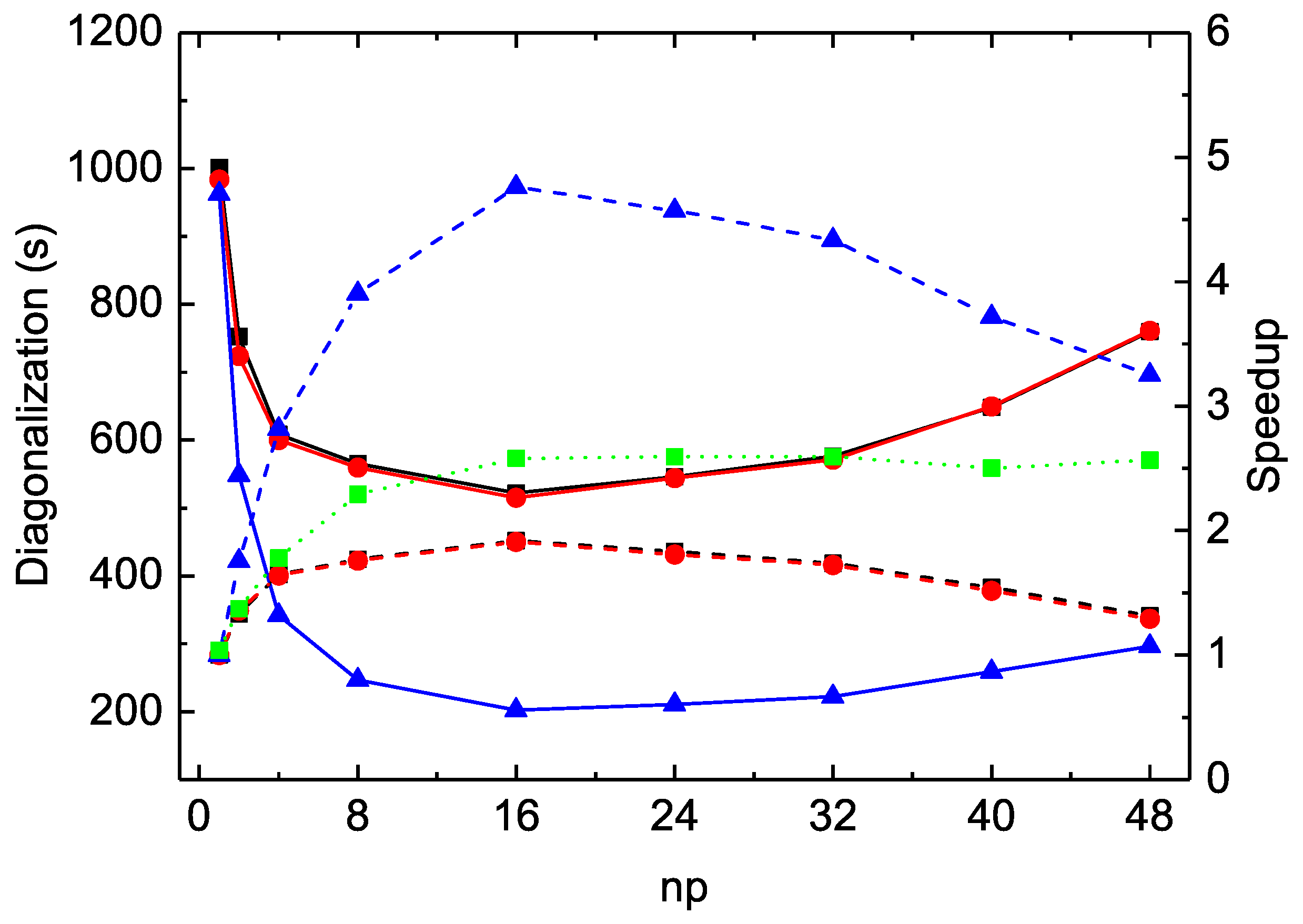
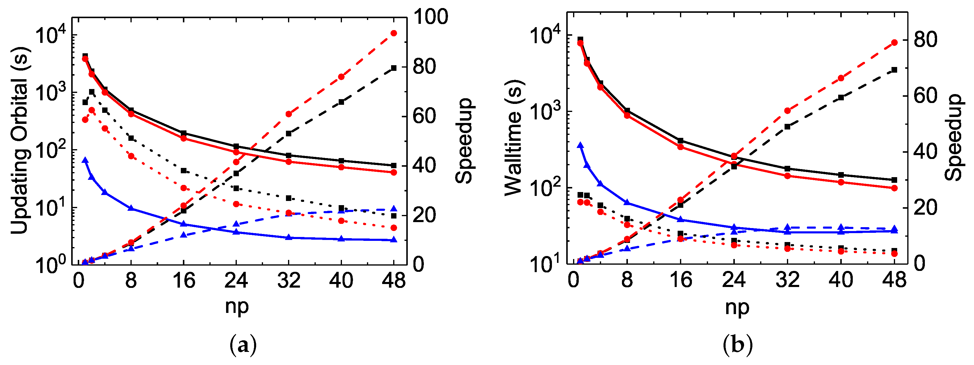
Based on the CPU times reported in Table 2 and Table 3, some comparisons are illustrated in Figure 1, Figure 2, Figure 3 and Figure 4. We discuss below the relative performances of the three codes.

Figure 1. MPI performances of the first diagonalization in the Mg VII $A{S}_3$-SCF calculations. Solid lines (left y axis): CPU times (T in s) of rmcdhf_mpi (squares), rmcdhf_mem_mpi (circles), and rmcdhf_mpi_FD (triangles) codes versus the number of MPI processes ($np$) (also listed in the first “SetH&Diag” line for each code of Table 2). Dashed lines (right y axis): speed-up factors for the three codes, with the same corresponding symbols, estimated from the ratios of $T(np=1)$ to others. Dotted line (right y axis) (square symbols): speed-up of rmcdhf_mpi_FD relative to rmcdhf_mpi, calculated as T(rmcdhf_mpi)/T(rmcdhf_mpi_FD).

Figure 2. MPI performances for updating orbitals in the Mg VII $A{S}_3$-SCF calculations. (a) Solid lines (left y axis): orbital updating CPU times (T in s) of rmcdhf_mpi (squares), rmcdhf_mem_mpi(circles), and rmcdhf_mpi_FD (triangles) codes versus the number of MPI processes ($np$) (also listed in the second “Update” line for each code of Table 2). Dashed lines (right y axis): speed-up factors for the three codes, with the same corresponding symbols, estimated from the ratios of $T(np=1)$ to others. (b) Speed-up factors of rmcdhf_mpi_FD relative to rmcdhf_mpi (squares) and to rmcdhf_mem_mpi (circles) calculated as T(rmcdhf_mpi)/T(rmcdhf_mpi_FD) and T(rmcdhf_mem_mpi)/T(rmcdhf_mpi_FD), respectively. Speed-up factors of rmcdhf_mem_mpi relative to rmcdhf_mpi (stars) calculated as T(rmcdhf_mpi)/T(rmcdhf_mem_mpi).

Figure 3. MPI performances for the code running times in the Mg VII $A{S}_3$-SCF calculations. (a) Solid (left y axis): walltimes (in s) for rmcdhf_mpi (squares), rmcdhf_mem_mpi (circles), and rmcdhf_mpi_FD (triangles) codes versus the number of MPI processes ($np$). Dashed lines (right y axis): speed-up factors for the three codes, with the same corresponding symbols, estimated from the ratios of $T(np=1)$ to others. (b): Speed-up factors of rmcdhf_mpi_FD relative to rmcdhf_mpi (squares) and to rmcdhf_mem_mpi (circles), respectively. Speed-up factors of rmcdhf_mem_mpi relative to rmcdhf_mpi (stars).

Figure 4. MPI performances of the codes for the Mg VII $A{S}_5$-SCF calculations. (a) Solid lines (left y axis): walltimes (in s) for rmcdhf_mpi (squares), rmcdhf_mem_mpi (circles) and rmcdhf_mpi_FD (triangles) codes versus the number of MPI processes ($np$). Dashed line (right y axis): speed-up factors for rmcdhf_mpi_FD (triangles) calculated as the ratios of $T(np=1)$ to others. Dotted lines (right y axis): speed-up factors for rmcdhf_mpi_FD relative to rmcdhf_mpi (squares) and to rmcdhf_mem_mpi (circles), respectively. (b) Solid lines (left y axis): orbital updating CPU times (T in s) for rmcdhf_mpi (squares), rmcdhf_mem_mpi (circles) and rmcdhf_mpi_FD (triangles) calculations. Dashed line (right y axis): speed-up factors (triangles) for rmcdhf_mpi_FD estimated from the ratios of $T(np=1)$ to others. The second “Update” times given in Table 3 are shown here. Dotted lines (right y axis): speed-up factors of rmcdhf_mpi_FD relative to rmcdhf_mpi (squares) and to rmcdhf_mem_mpi (circles), respectively.

As seen in Table 2 and Figure 1 for the $A{S}_3$ calculations, the MPI performances for diagonalization are unsatisfactory for all three codes. The largest speed-up factors are about $1.9$ for rmcdhf_mpi and rmcdhf_mem_mpi, and $4.7$ for rmcdhf_mpi_FD. The optimal numbers of MPI processes used for diagonalization are all around $np=16$ and the MPI performances deteriorate when $np$ exceeds 24. The CPU times of rmcdhf_mem_mpi and rmcdhf_mpi are very similar. Compared to these two codes, the CPU time of rmcdhf_mpi_FD is reduced by a factor of ≃2.5 with $np\ge 16$, thanks to the additional parallelization described in Section 2. 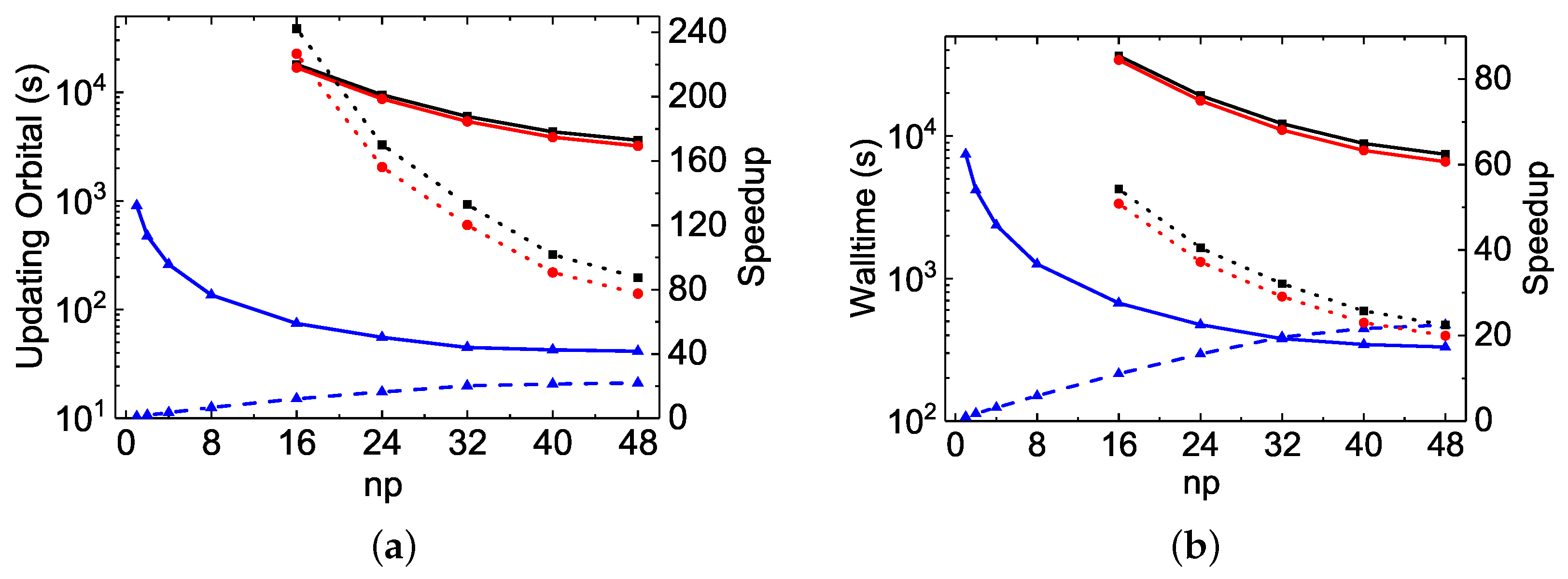The speed-up efficiency of rmcdhf_mpi_FD relative to rmcdhf_mpi increases slightly with the size of the CSF expansion. As seen from the first line of Table 3, the CPU time gain factor reaches $\approx 3$ for the calculations using the $A{S}_5$ orbital set. It should be noted that the CPU times to set the Hamiltonian matrix are negligible in all three codes, being tens of times shorter than those for the first search of eigenpairs. The eigenpairs are searched three times, and the corresponding CPU times are included in the three rows labeled “SetH&Diag”. As seen in Table 3, the first “SetH&Diag” CPU time is 945 s in the rmcdhf_mpi_FD $A{S}_5$ calculation with $np=48$, consisting of 14 and 931 s, respectively, for the matrix construction and diagonalization. For the subsequent two “SetH&Diag”, the matrix construction CPU times are still about 14 s, whereas those for diagonalization are, respectively, reduced to 34 and 26 s because the mixing coefficients are already converged. If the present calculations would be initialized by Thomas–Fermi or hydrogen-like approximations, these CPU times should reach about 900 s.

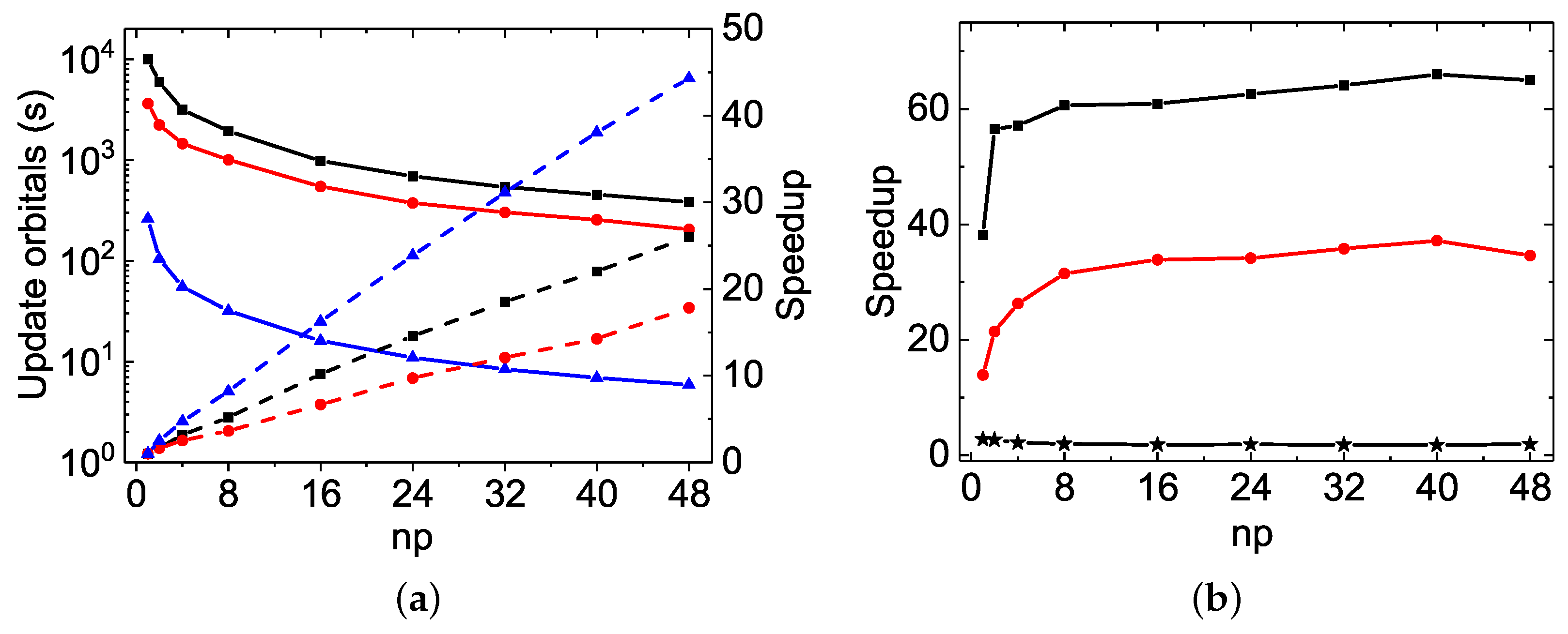
As far as the orbital updating process is concerned, the MPI performances of the three codes scale very well. The linearity is indeed attained even with $np=48$ or more, as seen in Figure 2a and Figure 4b. The speed-up factors with $np=48$ are, respectively, 26.0, 17.8 and 44.3 for the rmcdhf_mpi, rmcdhf_mem_mpi and rmcdhf_mpi_FD$A{S}_3$ calculations, while it is 43.2 for the $A{S}_5$ calculation using rmcdhf_mpi_FD. The slopes obtained by a linear fit of the speed-up factors as a function of np are, respectively, $0.53$, $0.35$, and $0.93$ for the rmcdhf_mpi, rmcdhf_mem_mpi, and rmcdhf_mpi_FD$A{S}_3$ calculations, while it reaches 0.91 for the rmcdhf_mpi_FD$A{S}_5$ calculation. In the $A{S}_3$ calculations, compared to rmcdhf_mpi and rmcdhf_mem_mpi, the rmcdhf_mpi_FD CPU times for updating the orbitals with $np\ge 8$ are, respectively, reduced by factors $(60-65)$ and $(31-37)$, as seen in Figure 2b. The corresponding reduction factors are $(57-69)$ and $(36-43)$ for the $A{S}_5$ calculations, as seen in Figure 4b. These large CPU time-saving factors result from the new strategy developed to calculate the potentials, as implemented in rmcdhf_mpi_FD, and described in Section 3.2. Unlike the diagonalization part, the memory version rmcdhf_mem_mpi brings about some interesting improvements over rmcdhf_mpi: the orbital updating CPU times are indeed reduced by a factor of 2 and 1.6 for the $A{S}_3$ and $A{S}_5$ calculations, respectively.

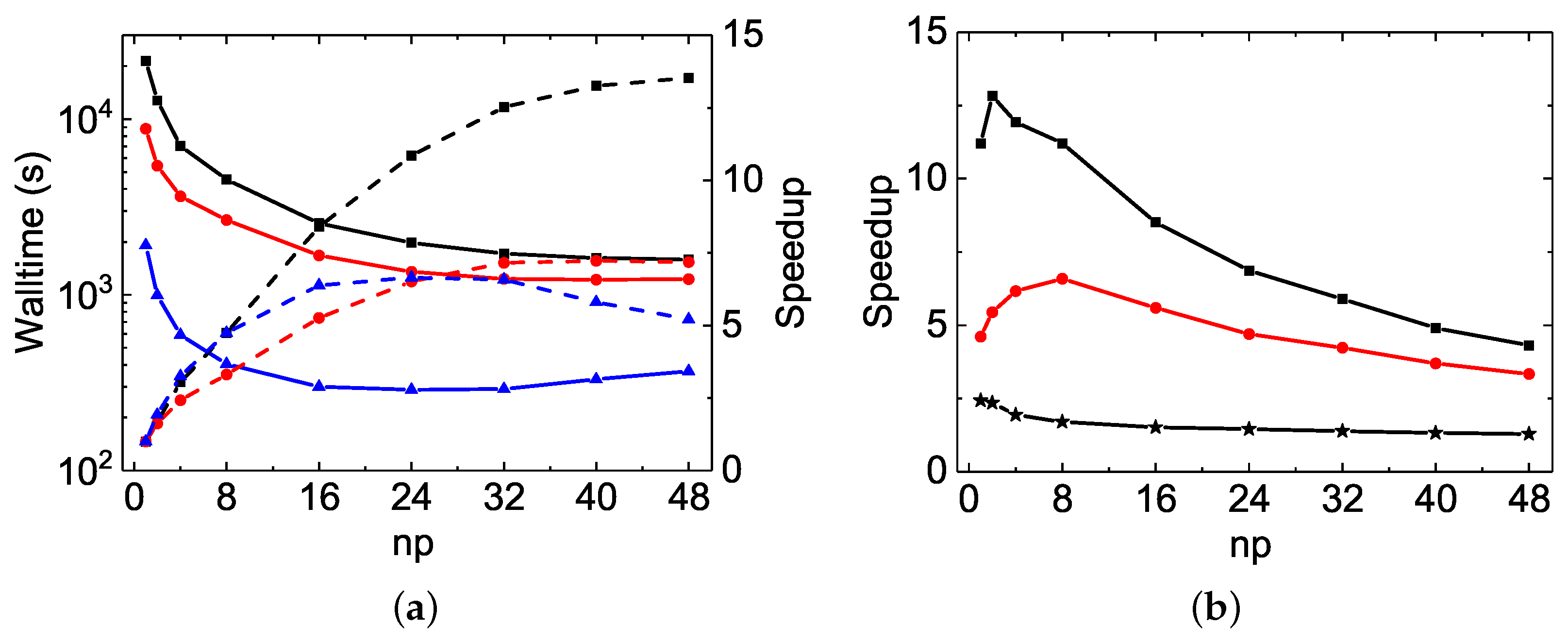
The MPI performances for the “walltimes” are different from each other among the three codes. As seen in Table 2 and Table 3, the orbital updating CPU times are predominant in most of the rmcdhf_mpi and rmcdhf_mem_mpi MPI calculations, whereas the diagonalization CPU times dominate in all rmcdhf_mpi_FD MPI calculations for all np values. Hence, as seen in Figure 3a and Figure 4a, the global MPI performance of rmcdhf_mpi_FD is similar to the one achieved for diagonalization. The maximum speed-up factors are, respectively, about 6.6 and 7.3 for the $A{S}_3$ and $A{S}_5$ calculations, both with $np$ = 16–32, though the “Update” CPU times could be reduced by factors of 44 or 43 with $np=48$, as shown above. The speed-ups increase along with np in the rmcdhf_mpi and rmcdhf_mem_mpi$A{S}_3$ calculations, being, respectively, about 13.5 and 7.2 with $np=48$. As shown in Figure 3b, comparing to rmcdhf_mpi, the walltimes are, respectively, reduced by a factor of 11.2 and 4.3 in rmcdhf_mpi_FD $A{S}_3$ calculations using $np=8$ and $np=48$, while the reduction factors are, respectively, 15 and 4.8 for the $A{S}_5$ calculations, as shown in Figure 4a. The corresponding speed-up factors of rmcdhf_mpi_FD relative to rmcdhf_mem_mpi are smaller by a factor of 1.5, as rmcdhf_mem_mpi is 1.5 times faster than rmcdhf_mpi, as seen in Figure 3b.

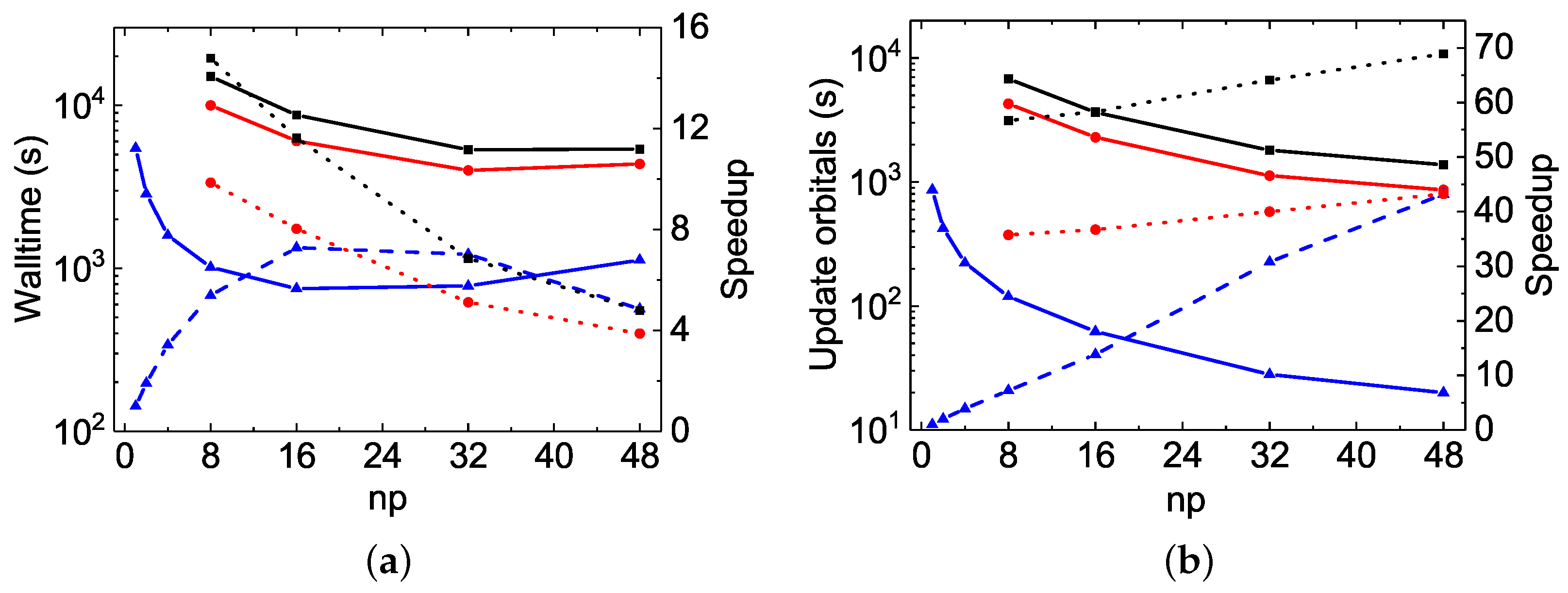
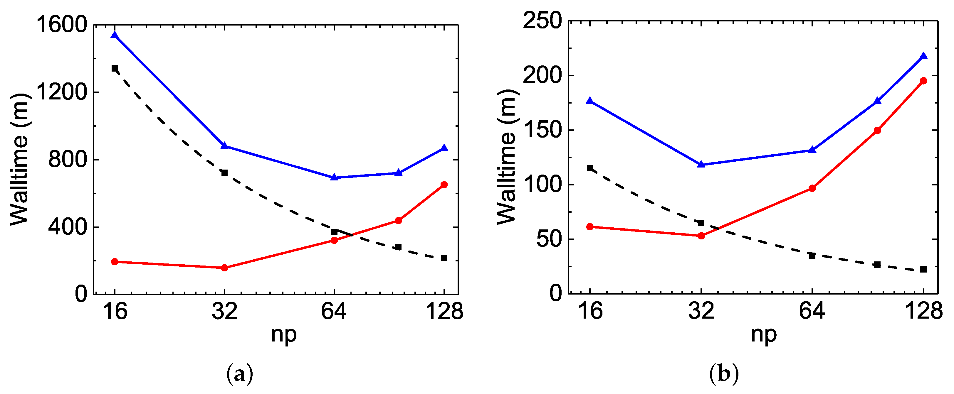
As mentioned above, the total CPU times for diagonalization reported in Table 2 and Table 3 (see rows labeled “Sum(SetH&Diag)”) are dominated by the first diagonalization, as the initial radial functions are taken from the converged calculations. In SCF calculations initialized by Tomas–Fermi or screened Hydrogenic approximations, more computation efforts have to be devoted to subsequent diagonalization during the SCF iterations. It is obvious that the limited MPI performance for diagonalization is the bottleneck in rmcdhf_mpi_FD calculations. As seen in Table 2 and Table 3 and Figure 3a and Figure 4a, more CPU time is required if np exceeds the optimal number of cores for diagonalization, which is generally in the range of 16–32. In rmcdhf_mpi and rmcdhf_mem_mpi calculations, the inefficiency of the orbital-updating procedure is another bottleneck, though this limitation may be alleviated by using more cores to perform the SCF calculations. However, this kind of alleviation would be eventually prohibited by the limited MPI performance of diagonalization. As seen in Table 3 and Figure 4a for the rmcdhf_mpi and rmcdhf_mem_mpi $A{S}_5$ calculations, the walltimes with $np=48$ are longer than those with $np=32$, though the CPU times for updating the orbitals are still reduced significantly in the former calculation.

3.3.2. Be I

To further understand the inefficiency of the orbital updating process in both rmcdhf_mpi and rmcdhf_mem_mpi codes, the second test case is carried out for a rather simple system, i.e., Be I. The calculations are performed to target the lowest 99 levels arising from the configurations $\left(1s^2\right)2l{n}^{\prime }{l}^{\prime }$ with $n^{\prime }\le 7$. The 99 levels are distributed over 15 $J^{\pi }$ blocks, i.e., $0^{+},0^{-},\cdots ,7^{+}$, with the largest numbers of 12 for $1^{-}$ and $2^{+}$ blocks. The MCDHF calculations are performed simultaneously for both even and odd parity states. The largest CSF space contains 55 166 CSFs formed by SD excitation up to $15\left(spdfg\right)14\left(hi\right)13\left(kl\right)$ orbitals from all the targeted states distributed over the above 15 $J^{\pi }$ blocks, with the largest size of 4 868 for $4^{+}$. The orbitals are also optimized with a layer-by-layer strategy. The CPU times recorded for the calculations using $9\left(spdfghikl\right)$ and $15\left(spdfg\right)14\left(hi\right)13\left(kl\right)$ orbital sets are given in Table 4 and Table 5. These calculations are hereafter labeled $n=9$ and $n=15$. The corresponding sizes of mcp.XXX files are, respectively, 760 MB and 19 GB. As the rmcdhf_mpi and rmcdhf_mem_mpi $n=15$ calculations are time-consuming, they are only performed with $np\ge 16$.

Table 4. CPU times (in s) for the Be I $n=9$ SCF calculations using the rmcdhf_mpi, rmcdhf_mem_mpi and rmcdhf_mpi_FD codes as a function of the number of MPI processes ($np$). See text for the label meanings.

np	1	2	4	8	16	24	32	40	48
				rmcdhf_mpi
SetH&Diag	73.43	42.57	25.77	15.98	9.61	8.20	7.13	7.34	7.83
				Iteration 1
SetCof + LAG	3 441.24	1 858.12	905.13	386.56	153.14	89.56	61.99	50.20	41.14
IMPROV	821.38	454.10	225.33	100.92	41.49	25.73	18.21	14.76	12.38
Update	4 262.62	2 312.22	1 130.46	487.48	194.63	115.29	80.20	64.96	53.51
SetH&Diag	71.50	40.70	23.85	14.23	7.73	6.30	5.32	5.20	5.38
				Iteration 2
SetCof + LAG	3 440.46	1 857.90	903.92	386.53	153.12	89.48	61.97	49.95	41.20
IMPROV	821.16	453.98	225.12	100.91	41.45	25.72	18.20	14.76	12.37
Update	4 261.62	2 311.88	1 129.04	487.43	194.57	115.20	80.18	64.71	53.57
SetH&Diag	71.67	40.72	23.82	14.03	7.72	6.07	5.30	5.20	5.44
Sum(SetH&Diag)	216.60	123.99	73.44	44.24	25.06	20.57	17.75	17.74	18.65
Sum(Update)	8 524.24	4 624.10	2 259.50	974.91	389.20	230.49	160.38	129.67	107.08
Walltime	8 741	4 748	2 333	1 019	414	251	178	147	126
				rmcdhf_mem_mpi
SetH&Diag	70.68	41.05	24.64	15.57	8.97	7.99	7.35	7.29	7.43
				Iteration 1
SetCof + LAG	3 065.84	1 656.84	795.63	329.83	123.75	70.08	47.42	37.94	30.53
IMPROV	741.20	410.89	201.45	88.74	35.15	21.54	15.06	12.19	10.10
Update	3 807.03	2 067.72	997.09	418.56	158.90	91.62	62.48	50.12	40.63
SetH&Diag	69.06	39.42	23.04	13.68	7.49	5.93	5.22	5.12	5.32
				Iteration 2
SetCof + LAG	3 065.78	1 656.36	795.29	329.60	123.63	69.96	47.37	37.91	30.56
IMPROV	741.54	410.94	201.15	88.73	35.14	21.51	15.06	12.18	10.10
Update	3 807.32	2 067.29	996.44	418.33	158.77	91.47	62.43	50.09	40.66
SetH&Diag	69.10	39.31	22.92	13.67	7.49	5.91	5.19	5.07	5.40
Sum(SetH&Diag)	208.84	119.78	70.60	42.92	23.95	19.83	17.76	17.48	18.15
Sum(Update)	7 614.35	4 135.01	1 993.53	836.89	317.67	183.09	124.91	100.21	81.29
Walltime	7 833	4 260	2 068	881	342	203	143	118	99
				rmcdhf_mpi_FD
SetH&Diag	68.82	39.33	23.11	13.82	8.92	7.43	6.83	7.14	7.30
NXA&NYA	10.98	7.52	5.03	3.21	2.45	2.34	2.48	2.84	3.29
				Iteration 1
SetTVCof	2.21	1.17	0.62	0.32	0.16	0.11	0.08	0.07	0.06
WithoutMCP	1.69	0.50	0.26	0.14	0.08	0.05	0.04	0.03	0.03
WithMCP	7.39	4.43	2.93	1.70	0.96	0.70	0.53	0.44	0.39
SetLAG	43.21	21.89	11.50	5.96	3.16	2.29	1.85	1.79	1.75
SetCof + LAG	54.64	28.01	15.33	8.13	4.38	3.18	2.55	2.38	2.29
IMPROV	10.10	5.09	2.70	1.39	0.73	0.54	0.44	0.43	0.42
Update	64.74	33.10	18.03	9.52	5.11	3.72	2.98	2.81	2.71
SetH&Diag	67.71	38.12	22.05	12.76	7.71	6.02	5.20	5.08	5.30
				Iteration 2
SetTVCof	2.21	1.17	0.62	0.31	0.16	0.11	0.08	0.07	0.06
WithoutMCP	1.69	0.50	0.26	0.14	0.08	0.05	0.04	0.03	0.03
WithMCP	7.42	4.43	2.93	1.70	0.96	0.70	0.53	0.44	0.39
SetLAG	43.33	21.86	11.52	5.96	3.15	2.28	1.85	1.79	1.75
SetCof + LAG	54.71	27.97	15.35	8.12	4.37	3.17	2.53	2.38	2.29
IMPROV	10.13	5.09	2.70	1.38	0.73	0.54	0.43	0.42	0.41
Update	64.84	33.06	18.05	9.51	5.10	3.71	2.97	2.80	2.70
SetH&Diag	67.75	38.11	22.11	12.68	7.64	6.01	5.20	5.08	5.25
Sum(SetH&Diag)	204.28	115.56	67.27	39.26	24.27	19.46	17.23	17.30	17.85
Sum(Update)	129.58	66.16	36.08	19.03	10.21	7.43	5.95	5.61	5.41
Walltime	354	194	111	63	38	30	26	26	27

Table 5. CPU times (in s) for the Be I $n=15$ SCF calculations using the rmcdhf_mpi, rmcdhf_mem_mpi and rmcdhf_mpi_FD codes as a function of the number of MPI processes ($np$). See text for the label meanings.

	rmcdhf_mpi			rmcdhf_mem_mpi			rmcdhf_mpi_FD
np	16	32	48	16	32	48	16	32	48
SetH&Diag	153.13	89.00	74.25	147.02	85.08	72.15	150.04	85.14	72.63
NXA&NYA							80.17	52.07	57.96
					Iteration 1
SetTVCof							3.81	1.95	1.29
WithoutMCP							1.21	0.61	0.43
WithMCP							18.86	10.77	7.92
SetLAG							46.19	28.35	28.12
SetCof + LAG	16 363.36	5 402.80	3 235.58	15 296.31	4 869.14	2 850.56	70.75	42.75	39.52
IMPROV	1 662.70	569.32	390.06	1 578.91	527.69	360.42	3.76	2.29	2.24
Update	18 026.06	5 972.12	3 625.64	16 875.21	5 396.83	3 210.99	74.51	45.04	41.76
SetH&Diag	138.23	71.42	55.28	132.74	68.96	53.04	136.68	70.91	54.79
					Iteration 2
SetTVCof							3.81	1.94	1.31
WithoutMCP							1.21	0.61	0.42
WithMCP							18.86	10.78	7.93
SetLAG							46.19	28.29	28.00
SetCof + LAG	16 364.56	5 403.63	3 234.71	15 295.55	4 870.41	2 849.64	70.63	42.61	39.19
IMPROV	1 662.93	569.19	389.98	1 578.93	527.58	360.37	3.77	2.29	2.25
Update	18 027.48	5 972.82	3 624.69	16 874.48	5 397.99	3 210.00	74.40	44.90	41.44
SetH&Diag	137.86	71.35	55.03	132.37	68.86	52.82	136.66	70.62	54.62
Sum(SetH&Diag)	429.22	231.77	184.56	412.13	222.90	178.01	423.38	226.67	182.04
Sum(Update)	36 053.54	11 944.94	7 250.33	33 749.69	10 794.82	6 420.99	148.91	89.94	83.20
Walltime	36 484	12 177	7 435	34 181	11 028	6 606	672	379	331

In comparison to the Mg VII test case considered in Section 3.3.1 (see Table 1), the CSF expansions for Be I are much smaller, and fewer levels are targeted. Hence, fewer computational efforts are expected for the construction of a Hamiltonian matrix and the subsequent diagonalization. This is true for the diagonalization parts of all the calculations using various $np$ MPI processes. For example, the CPU times for searching for eigenpairs are tens of times smaller than those for building the Hamiltonian matrix, representing 14s out of 150s, as reported by the first “SetH&Diag” value given in Table 5 for the rmcdhf_mpi_FD calculation with $np=16$. These CPU times are negligible (<1 s) for the following two diagonalizations. Unlike the cases considered for Mg VII, the CPU times for setting the Hamiltonian matrix predominate in the three “SetH&Diag” values, being all around 136s in the $n=15$ calculations using $np=16$, as shown in Table 5. These large differences in CPU time distributions between our Mg II and Be I test cases arise from the fact that the $n=15$ expansion in Be I is built on a rather large set of orbitals, consisting of 171 Dirac one-electron orbitals, whereas the $A{S}_5$ expansion in Mg VII involves only 88 ones. The number of Slater integrals $R^k(ab,cd)$ possibly contributing to matrix elements is, therefore, much larger in Be I (95 451 319) than in Mg VII (6 144 958). Consequently, the three codes report very similar “SetH&Diag” and “Sum(SetH&Diag)” CPU times and all attain the maximum speed-up factors of about 10 around $np=32$, as seen in Table 4.

The MPI performances of the Be I $n=9$ calculations are shown in Figure 5. In general, a perfect MPI scaling is a speed-up factor equal to $np$. With respect to this, the speed-up factors observed in rmcdhf_mpi and rmcdhf_mem_mpi are unusual, being much larger than the corresponding $np$ values. For example, the speed-up factors of rmcdhf_mpi and rmcdhf_mem_mpi for the orbital updating calculations are 79.5 and 93.6 at $np=48$, while the corresponding slopes obtained from the linear fit of the speed-up factors as a function of $np$ are about 1.7 and 2.0, respectively. The corresponding reductions at $np=48$ for the code running times are 69.4 and 79.1, while the slopes are about 1.5 and 1.7, respectively. These reductions should be even larger for the $n=15$ calculations. A detailed analysis shows that the inefficiency of the sequential search method largely accounts for the above unexpected MPI performances. As mentioned in Section 3.2, the labels LABYk and LABXk are constructed and stored sequentially in NYA(:,a) and NXA(:,a) arrays, respectively. In the subsequent accumulations of the $y^k$ and $x^k$ coefficients, the sequential search method is employed to match the labels. As mentioned above, a large number of Slater integrals contribute to the Hamiltonian matrix elements in calculations using a large set of orbitals. They are also involved in the calculations of the potential. In general, the number of $x^k$ terms is much larger than the number of $y^k$ terms. For example, the largest number of the former is 196 513 for all the $n{g}_{9/2}$ orbitals while there are at most 3 916 $y^k$ terms for all the $n{i}_{11/2}$ orbitals in the $n=9$ calculations. Similarly, for the $n=15$ calculations, there are at most 2 191 507 $x^k$ terms and 17 328 $y^k$ terms, both for the $n{g}_{9/2}$ orbitals. These values correspond to the largest sizes of the one-dimension vectors NXA(:,a) and NYA(:,a). The sequential search from a large list is obviously more inefficient than from a small list, as the time complexity is $O\left(n\right)$. In the MPI calculations with small np values, for example $np=1$, the sequential search of the LABXk from the NXA(:,a) lists of over two million elements is very time-consuming. It is obvious that the sizes of NXA(:,a) in each MPI process decrease as $np$ increases, alleviating the inefficiency of the sequential search method, as also shown in Mg VII calculations. For example, when $np=48$, the size of $NXA(:,n{g}_{9/2})$ in each MPI process is reduced to 528 802 in the $n=15$ calculations, and consequently, the unusually high speed-up factors are attained with both rmcdhf_mpi and rmcdhf_mem_mpi.

Figure 5. MPI performances for the Be I 9($spdfghikl$)-SCF calculations. (a) Solid (left y axis): orbital updating CPU times (T in s) for rmcdhf_mpi (squares), rmcdhf_mem_mpi (circles), and rmcdhf_mpi_FD (triangles) codes versus the number of MPI processes ($np$). Dashed line (right y axis): speed-up factors of the three codes (with the same corresponding symbols) estimated as the ratios of $T(np=1)$ to others. Dotted line (right y axis): speed-up factors of rmcdhf_mpi_FD relative to rmcdhf_mpi (squares) and to rmcdhf_mem_mpi (circles), calculated as T(rmcdhf_mpi)/T(rmcdhf_mpi_FD) and T(rmcdhf_mem_mpi)/T(rmcdhf_mpi_FD), respectively. (b) Same as in (a), but for the walltimes.

In rmcdhf_mpi_FD, the above inefficiency is removed by using the binary search strategy from the sorted arrays NXA(:,a) and NYA(:,a), and this code benefits from some other improvements, as discussed in Section 3.2. As seen in Figure 5a and Figure 6a, the speed-up factors for updating the orbitals increase slightly along with $np$ and attain the value of about 22 for both the $n=9$ and $n=15$rmcdhf_mpi_FD calculations with $np=48$, while the corresponding reductions for the code running times are, respectively, 12.5 and 22.5, as seen in Figure 5b and Figure 6b. It should be mentioned that in the rmcdhf_mpi and rmcdhf_mem_mpi calculations, the “Sum(SetH&Diag)” CPU time values are all less than the “Sum(Update)” ones, as seen in Table 4 and Table 5. However, it is the opposite for the rmcdhf_mpi_FD calculations, with all “Sum(SetH&Diag)” CPU time values still larger than the “Sum(Update)” ones, as in Mg VII calculations. Comparing to rmcdhf_mpi, the code rmcdhf_mpi_FD reduces the CPU times required for updating the orbitals by a factor lying in the range of 38–20, with $np$ = 16–48 for the $n=9$ MCDHF calculations, while for the $n=15$ calculations, the corresponding reduction factors are in the range of 242–287. The corresponding reduction factor ranges for the code running times are, respectively, 11–4.7 and 54–22.5, as seen in Figure 5b and Figure 6b. One can conclude that the larger the scale of the calculations, the larger the CPU time reduction factors. Moreover, the lower the number of cores used, the larger the reduction factors obtained with rmcdhf_mpi_FD. These features become highly relevant for extremely large-scale MCDHF calculations if they have to be performed using a small number of cores due to the limited performance of diagonalization, as discussed in the above section.

Figure 6. MPI performances for the Be I 15($spdfg$)14($hi$)13($kl$)-SCF calculations. (a) Solid (left y axis): orbital updating CPU times (T in s) for rmcdhf_mpi (squares), rmcdhf_mem_mpi (circles), and rmcdhf_mpi_FD (triangles) codes versus the number of MPI processes ($np$). Dashed line (right y axis): speed-up factors of rmcdhf_mpi_FD (triangles) calculated as the ratios of $T(np=1)$ to others. Dotted line (right y axis): speed-up factors of rmcdhf_mpi_FD relative to rmcdhf_mpi (squares) and to rmcdhf_mem_mpi (circles), calculated as T(rmcdhf_mpi)/T(rmcdhf_mpi_FD) and T(rmcdhf_mem_mpi)/T(rmcdhf_mpi_FD), respectively. (b) Same as in (a), but for the walltimes.

3.3.3. Possible Further Improvements for rmcdhf_mpi_FD

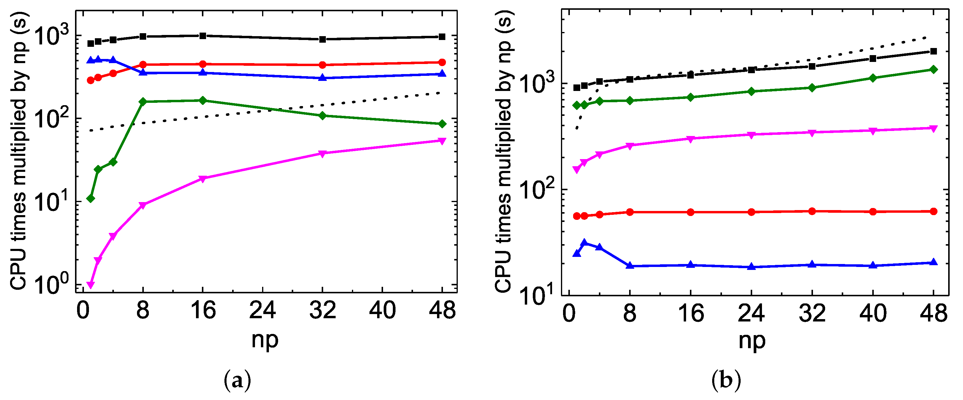
As discussed above, the MPI performances of rmcdhf_mpi_FD for updating orbitals scale well in Mg VII calculations. The speed-up factors roughly follow a scaling law of ≃$0.9np$ (see Figure 2b and Figure 4b). For the Be I calculations, however, as illustrated by Figure 5a and Figure 6a, the speed-up factor increases slightly with $np$ to attain a maximum value of 22. The partial CPU times for the orbital updating process, labeled “SetTVCof”, “WithoutMCP”, “WithMCP”, and “SetLAG”, are plotted in Figure 7, together with the total updating time labeled “Update”, for the Mg VII $A{S}_5$ and for the Be I $n=15$ calculations (these labels have been explained in Section 3.3.1.). The partial CPU times labeled “IMPROV” are not reported here, as they are generally negligible. It can be seen that the “SetTVCof” and “WithoutMCP” partial times dominate the total CPU times required for updating orbitals in Mg VII $A{S}_5$ calculations, and they all scale well along with $np$. In the Be I $n=15$ calculations, the partial “SetLAG” CPU times are predominant, and the remaining partial CPU times scale well. However, the scaling for both the partial “SetLAG” and total CPU times is worse than in Mg VII. Extra speed-up for “SetLAG” in Mg VII $A{S}_5$ calculations is observed. These different scalings can again be attributed to the fact that there is a large amount of $x^k$ terms contributing to the exchange potentials in Be I $n=15$ calculations, as mentioned above. For each $x^k\left(abcd\right)$ term, calculations of relativistic one-dimensional radial integrals $Y^k(bd;r)$ are performed on the grid with hundreds of r values. All these calculations are serial and are often repetitious for the same $Y^k(bd;r)$ integral associated with different $x^k\left(abcd\right)$ terms which differ from each other only by a and/or c orbitals. This kind of inefficiency could be improved by calculating all the needed $Y^k(bd;r)$ integrals in advance and storing them in arrays. This will be implemented in future versions of rmcdhf_mpi_FD codes.

Figure 7. MPI performances for the partial and total CPU times for updating the orbitals in (a) Mg VII $A{S}_5$ and (b) Be I $n=15$ calculations. Solid curves are the CPU times (in s) labeled “Update” (squares), “SetTVCof” (circles), “WithoutMCP” (up-triangles), “WithMCP” (down-triangles), and “SetLAG” (diamonds), respectively, for the first iteration of the rmcdhf_mpi_FD SCF calculations. (Some of them are also listed in Table 3 and Table 5). In addition, the “NXA&NYA” CPU times are also shown as the dotted line.

The MPI performances of the construction of $NYA$ and $NXA$ arrays are also displayed as dotted lines in Figure 7. As the distributed $LABYk$ and $LABXk$ values obtained by different MPI processes have to be collected, sorted and then re-distributed, the linear scaling begins to deteriorate at about 32 cores for the Be I $n=15$ calculations. Fortunately, this construction is realized only once, just before the SCF iterations. This slightly poor MPI performances should not be the bottleneck in large-scale MCDHF calculations.

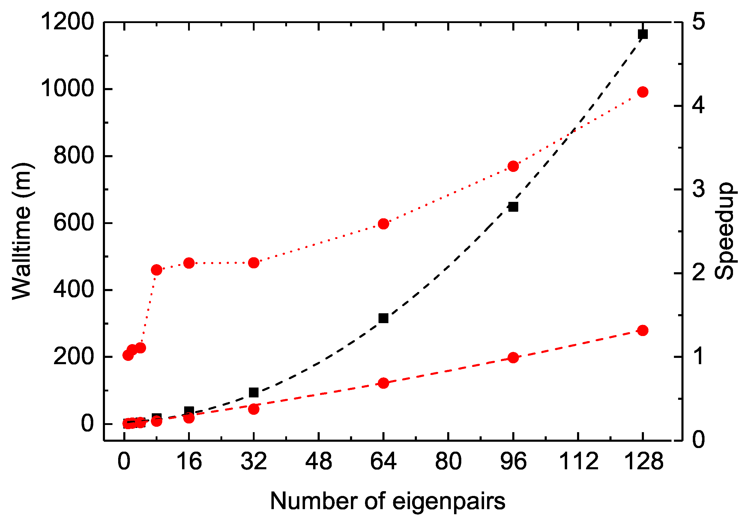
After a deep investigation of the procedures that could affect the MPI performances of rmcdhf_mpi_FD, one concludes that the poor performances of diagonalization could be the bottleneck for MCDHF calculations based on relatively large expansions consisting of hundreds of thousands of CSFs and targeting dozens of eigenpairs. We will discuss this issue in the next section.

4. Performance Tests for RCI Codes

The MCDHF calculations are generally followed by RCI calculations employing the GRASP rci and rci_mpi codes. In these calculations, larger CSF expansions than those considered in MCDHF calculations are used to capture higher-order electron correlation effects. Corrections to the Dirac–Coulomb Hamiltonian, such as the transverse photon interaction and the leading QED corrections, are also taken into account in this configuration interaction step, without affecting the one-electron orbitals. As mentioned in Section 1, we recently implemented in GRASP2018 [36] the original computational methodology based on configuration state function generators (CSFG) to build the Hamiltonian matrix. This strategy takes full advantage of the fact that the spin-angular integrals, such as the coefficients in Equation (5), are independent of the principal quantum numbers. In this approach, the CSFs space is divided into two parts, i.e., the labeling space and correlation space. The former typically accounts for the major correlation effects due to close degenerate and long-range rearrangements, while the latter typically accounts for short-range interactions and dynamical correlation. The orbitals set is also divided into two parts, i.e., a subset of labeling-ordered (LO) orbitals and a subset of symmetry-ordered (SO) orbitals [36]. The labeling CSFs are built with the LO orbitals only, generated by electron excitations (single (S), double (D), tripe (T), quadruple (Q), etc.) from an MR. The correlation CSFs are built with the LO orbitals together with SO orbitals, generated by only SD excitations also from the given MR. In the present implementation, two electrons at most are allowed to occupy the SO orbitals.

A CSFG of a given type is a correlation CSF in which one or two electrons occupy the SO orbitals with the highest principal quantum number allowed. Given a CSFG, a group of correlation CSFs can be generated by orbital de-excitations, within the SO orbitals set, that preserve the spin-angular coupling. The generated CSFs within the same group differ from each other only by the principal quantum numbers. The use of CSFGs makes it possible to restrict the spin-angular integration to a limited number of cases rather than being performed for each of the elements in the Hamiltonian matrix. Compared to ordinary RCI calculations employing rci_mpi, the CPU times are demonstrated to be reduced by factors of ten with the newly developed code, referred hereafter to as rci_mpi_CSFG. It is also found that the Breit contributions involving high orbital angular momentum (l) can be safely discarded. An efficient a priori condensation technique is also developed by using CSFG to significantly reduce the expansion sizes, with negligible changes to the computed transition energies. Some test calculations are presented for a number of atomic systems and correlation models with increasing sets of one-electron orbitals in [36]. Compared to the original GRASP2018 rci_mpi program, the larger the scale of the calculations, the larger the CPU time reduction factors will be with rci_mpi_CSFG. The latter is, therefore, very suitable for extremely large-scale calculations. Here we focus on the MPI performances of rci_mpi_CSFG and rci_mpi.

The MPI performance test calculations are performed for the $2^{+}$ block in Ne VII using the $A{S}_5$ orbitals set, i.e., $10\left(spdfghi\right)$. As in the MCDHF calculations, all the possible $\left(1s^2\right)2l^3{n}^{\prime }{l}^{\prime }$ with $2\le n^{\prime }\le 5$ configurations define the MR. The correlation CSFs are formed by SD excitations from this MR, allowing at most one electron excitation from the 1s subshell. These CSF expansions model both the VV and CV electron correlation. The number of resulting CSFs is $n_c$ = 2 112 922. This expansion is used in the rci_mpi calculation.

In the rci_mpi_CSFG calculation, all the $n\le 5$ orbitals are treated as LO orbitals, while the others are regarded as SO orbitals. The CSFs are generated as in the rci_mpi calculation. The labeling space contains 95 130 CSFs, while there are 197 480 CSFGs within the correlation space spanning 2 017 792 correlation CSFs. The total number of the original CSF expansion, $n_c$ is reproduced by adding the sizes of the labeling and correlation spaces, i.e., 95 130 + 2 017 792 = 2 112 922, as it should be. However, the program rci_mpi_CSFG reads a file of only $n_c^{\prime }$ = 292 610 CSFs, corresponding to the total of the labeling CSFs (95 130) and CSFGs (197 480). The size is reduced by the ratio $R=n_c/n_c^{\prime }\simeq 7$, compared to the file containing all the $n_c$ CSFs treated by rci_mpi. This ratio is very meaningful, being related to the performance enhancement of rci_mpi_CSFG, as the numbers of spin-angular integrations are, respectively, $n_c(n_c+1)/2$ and about $n_c^{\prime }(n_c^{\prime }+1)/2$ in the rci_mpi and rci_mpi_CSFG calculations. Ideally, relative to the former, a speed-up factor of $R^2$ is expected for the latter. It is obvious that this kind of outperformance is impossible to achieve because the spin-angular integration is not the whole computation load of RCI calculations.

The MPI performances of the rci_mpi and rci_mpi_CSFG can be realized from Table 6. All the MPI calculations are performed for the lowest 54 levels of $2^{+}$ in Ne VII, but using various $np$ cores in the range of 16–128 within a Linux server with two AMD EPYC 7763 64-Core Processors. Rather than using the zero-first approximation as in the above MCDHF calculations, here, all the matrix elements are calculated and taken into account in the RCI calculation. The disk space taken by the nonzero matrix elements is about 173 GB. The CPU times for building the Hamiltonian matrix, searching eigenpairs, and the sums are also shown in Figure 8. The former can be precisely reproduced by allometric scaling, i.e., $1121\times n{p}^{-0.822}$ and 16 005 $\times n{p}^{-0.894}$ both in minutes, respectively, for rci_mpi_CSFG and rci_mpi. This means that the CPU times for the matrix construction can be, respectively, reduced by factors of 1.77 and 1.86 if using double cores, implying that both rci_mpi and rci_mpi_CSFG have good MPI scaling to build the Hamiltonian matrix. However, the poor MPI scaling is again seen for diagonalization. The optimal $np$ values for the two codes are both around 32. The CPU times increase significantly with $np>32$. The rci_mpi and rci_mpi_CSFG diagonalization with $np=128$ is longer than with $np=32$ by factors of about 4.1 and 3.7, respectively. The different MPI scalings for the matrix construction and diagonalization are not unexpected. For the former, after each MPI process obtains the CSFs expansion, communications between different processes are not needed anymore. However, during the diagonalization procedure, a large amount of MPI communications are needed to ensure that each process has the same approximated eigenvector after every matrix-vector multiplication.

Table 6. CPU times (in s) for the construction of the Hamiltonian matrix (H), its diagonalization (D), and for the cumulated tasks (Sum) using rci_mpi and rci_mpi_CSFG for the $2^{+}$ block Mg VII calculations, as a function of the number of MPI processes ($np$).

	rci_mpi			rci_mpi_CSFG
np	H	D	Sum	H	D	Sum
16	1 342.08	194.87	1 536.95	114.97	61.45	176.42
32	722.68	158.54	881.22	64.98	53.11	118.09
64	370.86	321.84	692.70	34.85	96.66	131.51
96	281.45	439.48	720.93	26.80	149.45	176.25
128	216.50	651.80	868.30	22.42	195.08	217.50

Figure 8. MPI performances of rci_mpi and rci_mpi_CSFG. (a) CPU times (in min) for the construction of the Hamiltonian matrix (squares), its diagonalization (circles), and their sum (triangles) versus the number of MPI processes ($np$) for the $2^{+}$ block in Mg VII calculations with rci_mpi. The dashed curve is reproduced by an allometric fit, see text. (b) Same as in (a), but for calculations with rci_mpi_CSFG.

Consequently, considering both tasks (matrix construction and diagonalization), as seen in Table 6 and Figure 8, the optimal $np$ values for the whole code running times are in the ranges of 64–96 and 32–64 for rci_mpi and rci_mpi_CSFG, respectively. The latter outperforms the former by factors of 8.7 and 4.0 for the calculations using 16 and 128 cores, respectively. The best performance of rci_mpi_CSFG is 118 m using 32 cores, while it is 693 m using 64 cores for rci_mpi. The CPU time is reduced by a factor of 5.9 for rci_mpi_CSFG, but we should keep in mind that it uses half of the cores used by rci_mpi. This is more interesting for public servers. The outperformance of rci_mpi_CSFG is obviously due to the improvements in matrix construction and diagonalization, i.e., thanks to the implementation of CSFG and the additional parallelization, as discussed above. The CPU times needed for these two tasks are averagely reduced by about a factor of 10 and 3, respectively.

The scalability of the codes is also of interest if more and more eigenpairs are searched from a given Hamiltonian matrix. In Figure 9, the diagonalization CPU times are plotted versus $n_L$, the number of searched eigenpairs. These calculations were also performed for the $2^{+}$ block in Ne VII using 16 cores. We observe that the reported CPU times, $T\left(n_L\right)$ in minutes, with large enough $n_L$-values, can be well reproduced by a quadratic polynomial fit as $T\left(n_L\right)=5.20+0.519n_L+0.0662n_L^2$ and $T\left(n_L\right)=-3.46+1.54n_L+0.00538n_L^2$ for calculations with rci_mpi and rci_mpi_CSFG, respectively. For the latter, $T\left(n_L\right)$ is approximately linear in $n_L$ and the quadratic term is smaller by over one order of magnitude for this code than for rci_mpi. Consequently, the rci_mpi_CSFG outperforms rci_mpi more significantly as $n_L$ increases, reducing the diagonalization CPU times by a factor of 4.2 for $n_L=128$. This feature of rci_mpi_CSFG code is very helpful for large-scale spectrum calculation involving hundreds of levels.

Figure 9. CPU times (in min) for searching different numbers of eigenpairs of the $2^{+}$ block in Mg VII. Dashed lines: CPU times for rci_mpi (squares) and rci_mpi_CSFG (circles). The lines are reproduced by a quadratic polynomial fit. Dotted line (right y axis): speed-up factors of rci_mpi_CSFG relative to rci_mpi (circles).

5. Conclusions

In summary, the computation load of MCDHF calculations employing the GRASP rmcdhf_mpi code is generally divided into the orbital-updating process and the matrix diagonalization. The inefficiency found in the former part has been removed by redesigning the calculation of direct and exchange potentials, as well as Lagrange multipliers. Consequently, the CPU times may be significantly reduced by one or two orders of magnitude. For the second part, the additional parallelization of the diagonalization procedure may reduce the CPU times by about a factor of 3. The computation load of RCI calculations employing GRASP rci_mpi can also be divided into the Hamiltonian matrix construction and its diagonalization. In addition to the additional parallelization that improves the efficiency of the latter, the load of the former is reduced by a factor of ten or more thanks to the recently implemented computational methodology based on CSFG. Compared to the original rmcdhf_mpi and rci_mpi codes, the present modified versions, i.e., rmcdhf_mpi_FD and rci_mpi_CSFG cut down the whole computation loads of MCDHF and RCI calculations by several or tens of times, a factor that depends on the calculation scale governed by (i) the size of the CSF expansion, (ii) the size of the orbital set, (iii) the number of desired eigenpairs and (iv) the number of MPI processes used. In general, the larger the first three, the larger the CPU time reduction factors obtained with rmcdhf_mpi_FD and rci_mpi_CSFG. On the other hand, the smaller the number of used cores, the larger the reduction factors observed. These features make the rmcdhf_mpi_FD and rci_mpi_CSFG codes very suitable for extremely large-scale MCDHF and RCI calculations.

The MPI performances of the above four codes, as well as the memory version of rmcdhf_mpi, i.e., rmcdhf_mem_mpi, are carefully investigated. All codes have a good MPI scaling for the orbital updating process and the matrix construction step, respectively, in MCDHF and RCI calculations, whereas the MPI scaling for diagonalization is poor. If few eigenpairs are searched or very small CSFs expansions are employed, the MPI calculations may be performed using as many cores as possible. To obtain the best performance for large-scale calculation using hundreds of thousands or millions of CSFs expansion and targeting dozens of levels or more, the relative computation loads of diagonalization versus orbital update and matrix construction should be considered. As the latter two are, respectively, reduced significantly by rmcdhf_mpi_FD and rci_mpi_CSFG codes, the diagonalization computation load will often dominate. For such cases, the MPI calculations should be performed using the optimal number of cores for diagonalization, generally being around 32. The poor MPI scaling of diagonalization is obviously the bottleneck of rmcdhf_mpi_FD and rci_mpi_CSFG codes for precise spectrum calculations involving hundreds of levels. The way to improve the MPI scaling for diagonalization is unclear to us. An MPI/OpenMP hybridization might be helpful. By now, a temporary method is provided for large-scale RCI calculations. Firstly, the Hamiltonian matrix is calculated using as many cores as possible. The files storing the nonzero matrix elements are then re-distributed by a program to match the optimal diagonalization performances.

References

- Dyall, K.G.; Grant, I.P.; Johnson, C.T.; Parpia, F.A.; Plummer, E.P. Grasp—A General-purpose Relativistic Atomic-structure Program. Comput. Phys. Commun. 1989, 55, 425–456. [Google Scholar] [CrossRef]
- Grant, I.P.; McKenzie, B.J.; Norrington, P.H.; Mayers, D.F.; Pyper, N.C. An atomic multiconfigurational Dirac-Fock package. Comput. Phys. Commun. 1980, 21, 207–231. [Google Scholar] [CrossRef]
- Grant, I.P. Relativistic Quantum Theory of Atoms and Molecules. Theory and Computation (Atomic, Optical and Plasma Physics); Springer Science and Business Media, LLC: New York, NY, USA, 2007. [Google Scholar] [CrossRef]
- Froese Fischer, C.; Godefroid, M.; Brage, T.; Jönsson, P.; Gaigalas, G. Advanced multiconfiguration methods for complex atoms: I. Energies and wave functions. J. Phys. B At. Mol. Opt. Phys. 2016, 49, 182004. [Google Scholar] [CrossRef]
- Jönsson, P.; Godefroid, M.; Gaigalas, G.; Ekman, J.; Grumer, J.; Li, W.; Li, J.; Brage, T.; Grant, I.P.; Bieroń, J.; et al. An Introduction to Relativistic Theory as Implemented in GRASP. Atoms 2023, 11, 7. [Google Scholar] [CrossRef]
- Jönsson, P.; Gaigalas, G.; Bieroń, J.; Froese Fischer, C.; Grant, I.P. New version: Grasp2K relativistic atomic structure package. Comput. Phys. Commun. 2013, 184, 2197–2203. [Google Scholar] [CrossRef]
- Lindgren, I. The Rayleigh-Schrodinger perturbation and the linked-diagram theorem for a multi-configurational model space. J. Phys. B At. Mol. Phys. 1974, 7, 2441–2470. [Google Scholar] [CrossRef]
- Gu, M.F. The flexible atomic code. Can. J. Phys. 2008, 86, 675–689. [Google Scholar] [CrossRef]
- Gu, M.F. Energies of 1s22lq (1 ≤ q ≤ 8) states for Z ≤ 60 with a combined configuration interaction and many-body perturbation theory approach. At. Data Nucl. Data Tables 2005, 89, 267–293. [Google Scholar] [CrossRef]
- Gu, M.F.; Holczer, T.; Behar, E.; Kahn, S.M. Inner-Shell Absorption Lines of Fe VI-Fe XVI: A Many-Body Perturbation Theory Approach. Astrophys. J. 2006, 641, 1227–1232. [Google Scholar] [CrossRef]
- Si, R.; Guo, X.; Wang, K.; Li, S.; Yan, J.; Chen, C.; Brage, T.; Zou, Y. Energy levels and transition rates for helium-like ions with Z= 10–36. Astron. Astrophys. 2016, 592, A141. [Google Scholar] [CrossRef]
- Wang, K.; Chen, Z.B.; Zhang, C.Y.; Si, R.; Jönsson, P.; Hartman, H.; Gu, M.F.; Chen, C.Y.; Yan, J. Benchmarking Atomic Data for Astrophysics: Be-like Ions between B II and Ne VII. Astrophys. J. Suppl. Ser. 2018, 234, 40. [Google Scholar] [CrossRef]
- Wang, K.; Guo, X.; Liu, H.; Li, D.; Long, F.; Han, X.; Duan, B.; Li, J.; Huang, M.; Wang, Y.; et al. Systematic calculations of energy levels and transition rates of Be-like ions with Z= 10–30 using a combined configuration interaction and many-body perturbation theory approach. Astrophys. J. Suppl. Ser. 2015, 218, 16. [Google Scholar] [CrossRef]
- Wang, K.; Song, C.X.; Jönsson, P.; Ekman, J.; Godefroid, M.; Zhang, C.Y.; Si, R.; Zhao, X.H.; Chen, C.Y.; Yan, J. Large-scale Multiconfiguration Dirac–Hartree–Fock and Relativistic Configuration Interaction Calculations of Transition Data for B-like S xii. Astrophys. J. 2018, 864, 127. [Google Scholar] [CrossRef]
- Si, R.; Zhang, C.; Cheng, Z.; Wang, K.; Jönsson, P.; Yao, K.; Gu, M.; Chen, C. Energy Levels, Transition Rates and Electron Impact Excitation Rates for the B-like Isoelectronic Sequence with Z= 24–30. Astrophys. J. Suppl. Ser. 2018, 239, 3. [Google Scholar] [CrossRef]
- Li, J.; Zhang, C.; Del Zanna, G.; Jönsson, P.; Godefroid, M.; Gaigalas, G.; Rynkun, P.; Radžiūtė, L.; Wang, K.; Si, R.; et al. Large-scale Multiconfiguration Dirac–Hartree–Fock Calculations for Astrophysics: C-like Ions from O iii to Mg vii. Astrophys. J. Suppl. Ser. 2022, 260, 50. [Google Scholar] [CrossRef]
- Wang, K.; Si, R.; Dang, W.; Jönsson, P.; Guo, X.L.; Li, S.; Chen, Z.B.; Zhang, H.; Long, F.Y.; Liu, H.T.; et al. Calculations with spectroscopic accuracy: Energies and transition rates in the nitrogen isoelectronic sequence from Ar XII to Zn XXIV. Astrophys. J. Suppl. Ser. 2016, 223, 3. [Google Scholar] [CrossRef]
- Wang, K.; Jönsson, P.; Ekman, J.; Gaigalas, G.; Godefroid, M.; Si, R.; Chen, Z.; Li, S.; Chen, C.; Yan, J. Extended calculations of spectroscopic data: Energy levels, lifetimes, and transition rates for O-like ions from Cr XVII to Zn XXIII. Astrophys. J. Suppl. Ser. 2017, 229, 37. [Google Scholar] [CrossRef]
- Song, C.; Zhang, C.; Wang, K.; Si, R.; Godefroid, M.; Jönsson, P.; Dang, W.; Zhao, X.; Yan, J.; Chen, C. Extended calculations with spectroscopic accuracy: Energy levels and radiative rates for O-like ions between Ar XI and Cr XVII. At. Data Nucl. Data Tables 2021, 138, 101377. [Google Scholar] [CrossRef]
- Si, R.; Li, S.; Guo, X.; Chen, Z.; Brage, T.; Jönsson, P.; Wang, K.; Yan, J.; Chen, C.; Zou, Y. Extended calculations with spectroscopic accuracy: Energy levels and transition properties for the fluorine-like isoelectronic sequence with Z= 24–30. Astrophys. J. Suppl. Ser. 2016, 227, 16. [Google Scholar] [CrossRef]
- Li, J.; Zhang, C.; Si, R.; Wang, K.; Chen, C. Calculations of energies, transition rates, and lifetimes for the fluorine-like isoelectronic sequence with Z= 31- 35. At. Data Nucl. Data Tables 2019, 126, 158–294. [Google Scholar] [CrossRef]
- Wang, K.; Chen, Z.B.; Si, R.; Jönsson, P.; Ekman, J.; Guo, X.L.; Li, S.; Long, F.Y.; Dang, W.; Zhao, X.H.; et al. Extended relativistic configuration interaction and many-body perturbation calculations of spectroscopic data for the n ≤ 6 configurations in Ne-like ions between Cr XV and Kr XXVII. Astrophys. J. Suppl. Ser. 2016, 226, 14. [Google Scholar] [CrossRef]
- Zhang, X.; Del Zanna, G.; Wang, K.; Rynkun, P.; Jönsson, P.; Godefroid, M.; Gaigalas, G.; Radžiūtė, L.; Ma, L.; Si, R.; et al. Benchmarking Multiconfiguration Dirac–Hartree–Fock Calculations for Astrophysics: Si-like Ions from Cr xi to Zn xvii. Astrophys. J. Suppl. Ser. 2021, 257, 56. [Google Scholar] [CrossRef]
- Wang, K.; Jönsson, P.; Gaigalas, G.; Radžiūtė, L.; Rynkun, P.; Del Zanna, G.; Chen, C. Energy levels, lifetimes, and transition rates for P-like ions from Cr X to Zn XVI from large-scale relativistic multiconfiguration calculations. Astrophys. J. Suppl. Ser. 2018, 235, 27. [Google Scholar] [CrossRef]
- Song, C.; Wang, K.; Del Zanna, G.; Jönsson, P.; Si, R.; Godefroid, M.; Gaigalas, G.; Radžiūtė, L.; Rynkun, P.; Zhao, X.; et al. Large-scale Multiconfiguration Dirac–Hartree–Fock Calculations for Astrophysics: n = 4 Levels in P-like Ions from Mn xi to Ni xiv. Astrophys. J. Suppl. Ser. 2020, 247, 70. [Google Scholar] [CrossRef]
- Wang, K.; Song, C.X.; Jönsson, P.; Del Zanna, G.; Schiffmann, S.; Godefroid, M.; Gaigalas, G.; Zhao, X.H.; Si, R.; Chen, C.Y.; et al. Benchmarking atomic data from large-scale multiconfiguration Dirac–Hartree–Fock calculations for astrophysics: S-like ions from Cr ix to Cu xiv. Astrophys. J. Suppl. Ser. 2018, 239, 30. [Google Scholar] [CrossRef]
- Wang, K.; Jönsson, P.; Del Zanna, G.; Godefroid, M.; Chen, Z.; Chen, C.; Yan, J. Large-scale Multiconfiguration Dirac–Hartree–Fock Calculations for Astrophysics: Cl-like Ions from Cr viii to Zn xiv. Astrophys. J. Suppl. Ser. 2019, 246, 1. [Google Scholar] [CrossRef]
- Zhang, C.Y.; Wang, K.; Godefroid, M.; Jönsson, P.; Si, R.; Chen, C.Y. Benchmarking calculations with spectroscopic accuracy of excitation energies and wavelengths in sulfur-like tungsten. Phys. Rev. A 2020, 101, 032509. [Google Scholar] [CrossRef]
- Zhang, C.Y.; Wang, K.; Si, R.; Godefroid, M.; Jönsson, P.; Xiao, J.; Gu, M.F.; Chen, C.Y. Benchmarking calculations with spectroscopic accuracy of level energies and wavelengths in W LVII–W LXII tungsten ions. J. Quant. Spectrosc. Radiat. Transf. 2021, 269, 107650. [Google Scholar] [CrossRef]
- Zhang, C.Y.; Li, J.Q.; Wang, K.; Si, R.; Godefroid, M.; Jönsson, P.; Xiao, J.; Gu, M.F.; Chen, C.Y. Benchmarking calculations of wavelengths and transition rates with spectroscopic accuracy for W xlviii through W lvi tungsten ions. Phys. Rev. A 2022, 105, 022817. [Google Scholar] [CrossRef]
- Guo, X.; Li, M.; Zhang, C.; Wang, K.; Li, S.; Chen, Z.; Liu, Y.; Zhang, H.; Hutton, R.; Chen, C. High accuracy theoretical calculation of wavelengths and transition probabilities in Se-through Ga-like ions of tungsten. J. Quant. Spectrosc. Radiat. Transf. 2018, 210, 204–216. [Google Scholar] [CrossRef]
- Guo, X.; Li, M.; Si, R.; He, X.; Wang, K.; Dai, Z.; Liu, Y.; Zhang, H.; Chen, C. Accurate study on the properties of spectral lines for Br-like W39+. J. Phys. At. Mol. Opt. Phys. 2017, 51, 015002. [Google Scholar] [CrossRef]
- Guo, X.; Grumer, J.; Brage, T.; Si, R.; Chen, C.; Jönsson, P.; Wang, K.; Yan, J.; Hutton, R.; Zou, Y. Energy levels and radiative data for Kr-like W38+ from MCDHF and RMBPT calculations. J. Phys. At. Mol. Opt. Phys. 2016, 49, 135003. [Google Scholar] [CrossRef]
- Froese Fischer, C.; Gaigalas, G.; Jönsson, P.; Bieroń, J. GRASP2018—A Fortran 95 version of the general relativistic atomic structure package. Comput. Phys. Commun. 2019, 237, 184–187. [Google Scholar] [CrossRef]
- Gaigalas, G. Commits on Feb 2, 2022, commit/77aa600ab02b58718b9c5a82ce9e6c638cc09921. Available online: https://www.github.com/compas/grasp2018 (accessed on 20 November 2022).
- Li, Y.T.; Wang, K.; Si, R.; Godefroid, M.; Gaigalas, G.; Chen, C.Y.; Jönsson, P. Reducing the Computational Load—Atomic Multiconfiguration Calculations based on Configuration State Function Generators. Comput. Phys. Commun. 2022, 283, 108562. [Google Scholar] [CrossRef]
- Davidson, E.R. Iterative Calculation of A Few of Lowest Eigenvalues and Corresponding Eigenvectors of Large Real-symmetric Matrices. J. Comput. Phys. 1975, 17, 87–94. [Google Scholar] [CrossRef]
- Stathopoulos, A.; Froese Fischer, C. A Davidson program for finding a few selected extreme eigenpairs of a large, sparse, real, symmetric matrix. Comput. Phys. Commun. 1994, 79, 268–290. [Google Scholar] [CrossRef]
- Edmonds, A. Angular Momentum in Quantum Mechanics; Princeton University Press: Princeton, NJ, USA, 1957. [Google Scholar]
- Parpia, F.A.; Froese Fischer, C.; Grant, I.P. GRASP92: A package for large-scale relativistic atomic structure calculations. Comput. Phys. Commun. 1996, 94, 249–271. [Google Scholar] [CrossRef]
- Gaigalas, G.; Rudzikas, Z.; Froese Fischer, C. An efficient approach for spin - angular integrations in atomic structure calculations. J. Phys. B At. Mol. Opt. Phys. 1997, 30, 3747. [Google Scholar] [CrossRef]
- Gaigalas, G.; Fritzsche, S.; Grant, I.P. Program to calculate pure angular momentum coefficients in jj-coupling. Comput. Phys. Commun. 2001, 139, 263–278. [Google Scholar] [CrossRef]
- Gaigalas, G. A Program Library for Computing Pure Spin-Angular Coefficients for One- and Two-Particle Operators in Relativistic Atomic Theory. Atoms 2022, 10, 129. [Google Scholar] [CrossRef]
- Gustafsson, S.; Jönsson, P.; Froese Fischer, C.; Grant, I.P. Combining multiconfiguration and perturbation methods: Perturbative estimates of core–core electron correlation contributions to excitation energies in Mg-like iron. Atoms 2017, 5, 3. [Google Scholar] [CrossRef]
- Gaigalas, G.; Rynkun, P.; Radžiūtė, L.; Kato, D.; Tanaka, M.; Jönsson, P. Energy Level Structure and Transition Data of Er2+. Astrophys. J. Suppl. Ser. 2020, 248, 13. [Google Scholar] [CrossRef]
Disclaimer/Publisher’s Note: The statements, opinions and data contained in all publications are solely those of the individual author(s) and contributor(s) and not of MDPI and/or the editor(s). MDPI and/or the editor(s) disclaim responsibility for any injury to people or property resulting from any ideas, methods, instructions or products referred to in the content. |
© 2023 by the authors. Licensee MDPI, Basel, Switzerland. This article is an open access article distributed under the terms and conditions of the Creative Commons Attribution (CC BY) license (https://creativecommons.org/licenses/by/4.0/).