Abstract
The strong-field approximation (SFA) has been widely applied in the literature to model the ionization of atoms and molecules by intense laser pulses. A recent re-formulation of the SFA in terms of partial waves and spherical tensor operators helped adopt this approach to account for realistic atomic potentials and pulses of different shape and time structure. This re-formulation also enables one to overcome certain limitations of the original SFA formulation with regard to the representation of the initial-bound and final-continuum wave functions of the emitted electrons. We here show within the framework of Jac, the Jena Atomic Calculator, how the direct SFA ionization amplitude can be readily generated and utilized in order to compute above-threshold ionization (ATI) distributions for many-electron targets and laser pulses of given frequency, intensity, polarization, pulse duration and carrier–envelope phase. Examples are shown for selected ATI energy, angular as well as momentum distributions in the strong-field ionization of atomic krypton. We also briefly discuss how this approach can be extended to incorporate rescattering and high-harmonic processes into the SFA amplitudes.
1. Introduction
During the past decades, strong-field ionization measurements in atoms and molecules have led to numerous insights into the electron dynamics on short time scales. In particular, several nonlinear optical processes, such as the above-threshold ionization (ATI, [1,2]), tunneling ionization, high-order harmonic generation (HHG, [3,4]), or the nonsequential double ionization (NSDI, [5]) have attracted much interest and can be readily controlled by tailoring the temporal shape and duration of ultrashort laser pulses. In ATI, for example, the energy and momentum distributions of photoelectrons are often recorded for different targets and (short) laser pulses of different frequency , intensity I, polarization , pulse duration (i.e., number of laser cycles, ), or by even steering the carrier–envelope phase . In contrast to the detailed modeling of the driving laser pulse, however, the target atoms are typically described in rather a simplified manner, and especially the initial state of the active electron is often just taken as a hydrogenic state [6,7]. Because of this and further simplifications in modeling the target atoms, many observations are still understood only qualitatively so far.
Figure 1a displays the prototypical geometry and observables of an ATI experiment. Here, atoms are exposed to an intense driving laser pulse with given intensity I, wavelength , ellipticity or, perhaps, even a superposition of such light fields. A detector D records the photoelectrons that are emitted due to the interaction of laser pulse with the target atoms. Routinely, the photoelectron energy distributions are recorded at a fixed detector position within the polarization plane (Figure 1b). The observed photoelectron energy spectra then exhibit ATI peaks that are spaced by the photon energy. If the detector position is varied within the polarization plane, azimuthal angular distributions can be recorded for photoelectrons of selected energy (Figure 1c). These angular distributions strongly depend not only on the shape of the driving laser pulse but also on the outgoing electron wave in the potential of the photoion. In addition, the full photoelectron momentum distributions are often measured within the polarization plane as shown in Figure 1d.
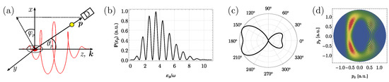
Figure 1.
ATI experiment and typical observables. (a) geometry of an ATI experiment: An atom is irradiated by a strong laser pulse (red) of intensity I and wavelength that propagates along the z-axis and is polarized with ellipticity within the plane. Due to the interaction with the laser field, a photoelectron is emitted with momentum in spherical coordinates and measured at the detector D. (b) For a given position of the detector within the polarization plane, the measured photoelectron energy distributions exhibit several ATI peaks that are just spaced by the photon energy. (c) For a few-cycle driving laser pulse, the angular distribution of photoelectrons with fixed energy reveals an asymmetry which encodes details of the pulse structure and the electron continuum. (d) In addition, full photoelectron momentum distributions are often recorded within the polarization plane.
While any reliable theory of the strong-field (ionization) processes from above must have its roots in the time-dependent Schrödinger equation, a direct (numerical) integration of this equation becomes unfeasible already for the three-dimensional motion of a single (active) electron in a static soft-core potential, not to speak about the many-electron nature of most targets [8]. Therefore, a number of analytical methods have been developed as well and nowadays provide good insights into the underlying electron dynamics. In particular, the strong-field approximation (SFA) [9,10,11] provides an efficient single-electron treatment and has become, despite several limitations in its original form, a very valuable tool for computing the ATI and HHG spectra for a wide range of laser parameters and targets [12,13,14]. Here, however, a re-formulation of the SFA in terms of partial waves and spherical tensors [15] is applied and help adopt this method towards modern strong-field measurements. This re-formulation enables one to incorporate all central features of the incident laser pulse as well as the electronic structure of the target atoms.
To support the analysis of different strong-field measurements, this work reports an implementation of the (direct) SFA amplitude in its partial-wave representation within the framework of Jac, the Jena Atomic Calculator [16]. This toolbox, which facilitates the (relativistic) computation of atomic structures and processes [17,18], has been expanded here in order to model the initial-bound and final-Volkov states in the computation of strong-field amplitudes. Apart from the active-electron waves, however, our implementation below is flexible also in choosing the polarization, shape (envelope) and even the CEP phase of the driving laser pulse. Indeed, all these features have been found to be (very) crucial to further adopt the theoretical modeling of strong-field ionization processes to ongoing experiments.
The paper is structured as follows: After a brief discussion of the SFA and the direct amplitude in terms of partial waves in Section 2, emphasis is placed on the implementation within the framework of Jac as well as the role of appropriate data structures for simplifying the communication with and within the program. Section 3 then explains and discusses how the different energy, angular and momentum distributions can be obtained quite readily by just specifying the initial and final levels of the target atom as well as the parameters of the laser pulse. This includes the choice of atomic potential and the Volkov states in the evaluation of the amplitudes. Finally, a short summary and conclusions are given in Section 4, with emphasis on possible extensions of the code towards rescattering phenomena, or the computation of harmonic spectra.
2. Strong-Field Amplitudes and Probabilities
2.1. Brief Account of the Strong-Field Approximation
The SFA has been known as perhaps the most straight avenue for modeling strong-field ionization processes and for analyzing most of the associated ATI spectra and momentum distributions. In this approximation, a (so-called) active electron is assumed to undergo a transition from its initial bound state into the laser-dressed continuum owing to its interaction with the laser pulse (cf. Figure 1a), while the motion of all other electrons of the target is typically assumed to be unaffected. Not much need to be said here about the basic SFA theory, which can be found in various texts [12,13]. In this approximation, the probability for the strong-field ionization of atoms and for finding a photoelectron with asymptotic momentum at the detector,
can then be expressed in terms of transition amplitudes as [6]
and where refers to the laser–electron interaction, the time evolution and to the atomic potential as seen by the outgoing electron.
Indeed, the two (strong-field) amplitudes and can be readily interpreted in terms of a (re-) scattered photoelectron and are often referred to as the direct and rescattering amplitudes, respectively. In this work, we shall focus especially on the direct amplitude that describes those photoelectrons which are directly released from the target atom by the laser potential, , and then freely propagate within the laser field as Volkov solution , until they reach the detector. Indeed, this amplitude often provides a good approximation for most strong-field ionization processes and, in particular, if the laser field is not linearly polarized. Typically, the following assumptions are made to further simplify the amplitude (2):
- The initial-bound state is entirely determined by the atomic potential and is not affected by the laser field.
- The photoelectron with asymptotic momentum arrives as plane-wave at the detector, i.e., .
- Once the electron is released from the atom, the atomic potential does not affect its (electronic) motion within the continuum.
Often, moreover, a Coulomb potential has been applied, in line with the ionization potential of the target atoms, and the initial state has been taken just as ground state orbital in this (Coulomb) potential. With these assumptions in mind, the momentum distribution of the photoelectrons can then be expressed by a closed (analytical) formula. Obviously, however, these assumptions neglect both a proper representation of the initial state of the atoms as well as the (static) potential of the photoion upon the outgoing electron wave (continuum) and, hence, quite major parts of the electronic structure of the target atoms.
Several, if not most, of these assumptions can be easily released, if the initial and final states are consequently expressed in terms of partial waves as typical for atomic structure theory [15]. In such a partial wave expansion, the representation of the initial bound and (Volkov) continuum states can be incorporated along with the parameterization of the short an intense laser pulses. It is this representation of the (direct) transition amplitude on which we shall focus in the implementation below and which paves the way for extending the strong-field theory towards the study of non-dipole contributions in light-atom interactions as well as towards many-particle correlations in strong-field ionization processes.
2.2. Partial-Wave Representation of Strong-Field Amplitudes
In the derivation of the SFA amplitude ((2) and (3)), indeed, no additional assumptions have to be made about the form of the atomic potential or about the potentials and of the driving laser field, but which—of course—affect the Volkov states . If, for the coupling of the radiation field, we restrict ourselves to the dipole approximation [] and the velocity gauge [], the vector potential of an elliptically-polarized laser pulse can be written in terms of its spherical tensor components as
and where denotes the (real-valued) amplitude, the pulse envelope, the fundamental frequency, and where refers to the carrier–envelope phase of the laser pulse. In this notation, moreover, the (complex) polarization unit vector
defines the orientation of the polarization ellipse in terms of the ellipticity . The vector potential (4) therefore implies already all the properties and of the laser field which can be controlled experimentally.
A partial-wave representation of the amplitudes ((2) and (3)) also enables one to adapt both the initial bound state and the final continuum state to the target potential of interest [15,19]. This is readily achieved, for instance, by using (self-consistent) solutions from atomic structure theory. For the outgoing photoelectron
moreover, one only needs to replace the partial wave in the expansion of a plane-wave Volkov state by the corresponding solutions of either a Coulomb–Volkov or distorted-Volkov state in order to account for a realistic potential of the target, including the associated Coulombic and non-Coulombic phase shifts [20,21]. Here, we shall provide only a brief discussion of the theory, just enough to follow our implementation below, while all further details are given in Refs. [15,19].
For the direct SFA transition amplitude (2), Equations (23) and (24) of reference [15] display a rather lengthy formula that is written in a basis of well-defined total angular momenta for the initially bound and the final (photo-) electron. This expression depends explicitly on the Volkov phase and all the parameters of the driving laser pulse, and it also accounts for the spatial dependence of the active electron in terms of the reduced one-particle matrix elements of the momentum operator, as typical for atomic structure theory. The advantage of such an expression in a spherical basis arises from the—prior and separate—integration over all radial and spherical coordinates. This expression therefore also enables one to readily incorporate and discuss different contributions from the electron–photon interaction and the representation of the active electron without any need to re-derive the transition amplitude(s) for every target potential and/or laser (pulse) configuration separately. Below, we shall focus especially upon realistic (single-electron) initial states and the improved representation of the continuum for the outgoing photoelectron. It is this partial-wave representation of the direct SFA amplitude which makes the present extension an integral part of the Jac toolbox and which goes well beyond of what has been used originally in the SFA. However, since the expression in Ref. [15] is still restricted to the electric-dipole approximation, it neither accounts for the magnetic field nor any spatial dependence of the electric field, though this can likely be done as well (cf. Section 4).
2.3. Implementation of the (Direct) Strong-Field Amplitude
Like in atomic structure theory, a partial-wave representation of all (strong-field) amplitudes enables one to deal quite independently with atomic potentials, the Volkov state for the outgoing electron or the laser–electron interaction in terms of the given laser parameters. Such a representation also helps identify the building blocks for computing the photoelectron spectra and/or momentum distributions, as they are observed experimentally. In the Jac toolbox, we therefore aim to distinguish between the target and laser parameters as the input of a computations, and the generated observables (spectra) as output. A simple access to all individual input parameters will enable us to compute the strong-field ionization amplitudes in quite different approximations. Although the current implementation is still restricted to the direct SFA amplitude in velocity gauge, the same or very similar building blocks will occur if other amplitudes or gauges are to be considered in the future. The use of partial waves and spherical tensors even ensures that these amplitudes can be readily combined with atomic structure codes to further include electronic correlations and relativistic contributions to the strong-field ionization studies.
Not much need to be said about Jac itself, the Jena Atomic Calculator [16] that supports atomic (structure) calculations of different kind and complexity and that has been summarized at various places [22,23,24]. Apart from energies and wave functions for open-shell atoms and ions, this toolbox also helps compute a good number of their excitation and decay processes. With the design and implementation of Jac [25], we moreover aim for establishing a descriptive language that (i) is simple enough for both, a seldom or more frequent use of this toolbox, (ii) emphasizes the underlying atomic physics and, furthermore, (iii) avoids most technical slang as common to many other electronic structure codes. The implementation of Jac is based on Julia [26,27], a recently developed programming language for scientific computing, and supports its use without much prior knowledge about neither the language nor the code itself.
Figure 2 displays a few selected atomic processes that are presently supported by Jac, and which are shown together with useful features and control parameters for calculating strong-field amplitudes. The set of parameters in the right panel of Figure 2 hereby indicates how between different pulses we shall distinguish in these computations geometries and/or gauges for the coupling of the radiation field, and as far they have been worked out until the present. In particular, the initial bound and final Volkov states of the (photo-) electron just appear in the reduced matrix elements and can be taken either as a hydrogenic orbital, scaled upon the ionization potential, or as realistic one-electron wave function. Here, the continuum orbitals are generated in the static potential of the photoion and with energies as measured at the detector [28].
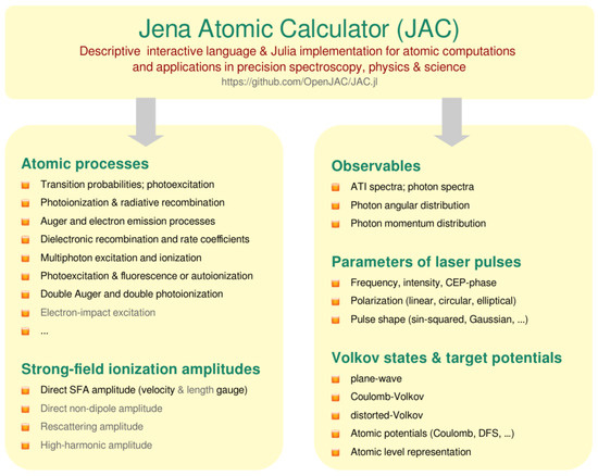
Figure 2.
Selected applications of the Jac toolbox that help calculate atomic structures and processes as well as strong-field ionization amplitudes in various approximations. Apart from choosing between typical strong-field observables, the Volkov states and the parameterization of the laser pulses can be controlled rather flexibly. See Refs. [16,25] for a detailed account of all other features of this toolbox.
Special care has to be taken about the envelope of the laser pulses. In a spherical-wave expansion, this envelope enters the direct amplitude in terms of (so-called) pulse-shape integrals and , cf. Ref. [15]. These one-dimensional, (time) integrals are often obtained numerically but can be evaluated also analytically for continuous beams and a few other forms of the envelope. In our implementation below, the envelope (shape) of the laser pulse is accessed by a proper (abstract) data type, quite similar to the frequency, intensity, number of cycles and the polarization of the incident pulses. In typical applications of Jac, one needs to select these parameters based on the given setup of the experiment and different practical considerations in order to keep the computations feasible.
2.4. Data Types for Modeling Photoelectron Distributions and Above-Threshold Experiments
From a physics viewpoint, we normally wish to trace back the simulation of different spectra and photoelectron distributions to just computing the (direct) SFA amplitude from above, though for specifically selected target atoms, approximation of wave functions and parameters of the laser pulse. Obviously, this requires simple access to all these data as well as special care to bring them together with the internal calls of the program. To facilitate the communication with and the data transfer within the program, the Jac toolbox is built upon a large number of data structures in order to specify useful and frequently recurring objects in such computations, and which also establish their language elements. Two prominent examples for such data structures, that frequently appear in atomic structure theory, are an Orbital for specifying the quantum numbers and radial components of single-electron orbital functions, or a Level for the full representation of an approximate initial or final bound state of the target atoms, and which itself comprises all information about the orbitals, the coupling of the angular momenta and the mixing of the many-electron target states. These target states are typically obtained self-consistently in a Dirac–Fock–Slater potential and hence are based on orbitals in line with the given target. Jac’s explicit set of data structures has been enlarged for the present update of the code by several types and now helps compute, analyze and explore the desired photoelectron spectra for different laser pulses and targets. In total, there are about 250 of these data structures in Jac, though most of them remain hidden to the user.
To model different strong-field ionization measurements, we wish (and need) to characterize especially the incident laser pulse in terms of its frequency, intensity, shape and polarization as well as the observables (spectra) to be simulated. In addition, we wish to control the target potentials and representation of the Volkov states in the strong-field amplitude. All this input is very central to the implementation and must be readily accessible by the given hierarchy of data structures. While we shall not explain these structures in all detail here, Figure 3 displays a few of them from Jac’s Pulse and StrongField modules. The abstract type Pulse.AbstractEnvelope (middle panel), for example, just deals with the envelope of the laser pulse and comprises various concrete types for specifying a particular shape, pulse duration or number of cycles. Similarly, the data type StrongField.AbstractSFAObservable enables one to specify the observable of choice and its resolution. All this information about the observable, target and pulse parameters finally define (an instance of) a StrongField.Computation (lower panel), and which can be utilized in Jac analogue to the previously implemented Atomic.Computation [16,29] or Cascade.Computation [30,31].
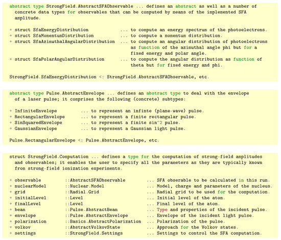
Figure 3.
Selected data structures of the Jac toolbox that help specify and perform a StrongField.Computation (lower panel). Apart from the observable of interest (upper panel), the nuclear model, radial grid as well as the initial and final level of the target atom, one needs to specify the properties of the laser pulse in terms of its beam type, envelope (middle panel) and the polarization of the incident light. Moreover, the user can select the Volkov state approach and a number of further settings. See Table 1 for other data types that are closely related to StrongField.Computations.
Finally, Table 1 displays several other data structures that are relevant as well for the computation and analysis of strong-field photoelectron distributions. They are explained only in brief, while further details can be obtained from Jac’s User Guide [25] or by just using Julia’s help facilities [32]. The definition and hierarchy of these data structures however nicely illustrate how they help implement different strong-field ionization scenarios and, hence, a wide range of potential applications in atomic and atto-second physics. In the next section, we make use of these data types to simulate various energy, angular and momentum distributions for a krypton target.

Table 1.
Selected data structures of the Jac toolbox that are relevant for StrongField.Computations. Here, only a brief explanation is given, while further details can be found by using Julia’s help facilities.
3. Energy and Momentum Distributions for Atomic Krypton
In the literature, the SFA has been frequently applied for comparing the energy and momentum distributions with experiments and for studying pulses and targets of quite a different sort. In these computations, more often than not, the active electron has initially been assumed to be in a hydrogenic state, and by just matching the ionization potential to the target of interest. However, such a simple approach provides only little insight into the role that the target atoms play in strong-field ionization. Here, we wish to demonstrate that our partial-wave representation of the SFA amplitude enables us to adopt the initial-bound and final-Volkov states to realistic target potentials. We also show how the ATI spectra and momentum distributions can be obtained for pulses of different intensity, polarization and pulse duration. All these computations are performed by applying the Jac toolbox [16], which integrates the electronic structure and a good deal of atomic processes within a single computational framework, and which has now been expanded to facilitate the simulation of strong-field ionization distributions. For the sake of convenience, all simulations below are performed for krypton ( 14 eV) and a right-circularly polarized, cycle driving laser pulse with wavelength nm, intensity W/cm and carrier–envelope phase . Here, we shall not compare our implementation with experiment or previous computations, which have been done recently for a number of other targets [19].
3.1. Above-Threshold Energy Spectra
Often, the observed ATI spectra can be qualitatively reproduced by simply using the SFA and plane-wave Volkov continuum states, since the peak structure of these photoelectron spectra itself arises from the interaction of the (quasi-) free electron with the electric field of the ionizing laser pulse. For these reasons, most energy spectra also exhibit distinct peaks, which are just spaced by the photon energy of the incident laser beam. These peaks become easily visible by measuring the photoelectron energy for a fixed azimuthal angle along some line in the polarization plane. Besides the selected laser parameters, these energy spectra depend of course also on the target atoms as well as on how the photoelectrons are described on their way to the detector, including the Volkov continuum and, possibly, even a re-scattering of the photoelectrons.
The ATI energy spectra of the strong-field photoelectrons can be modeled also by the present extension to the Jac toolbox. Figure 4 displays the (Julia) input which needs to be prepared by the user and which enables one to calculate such spectra for different targets and pulses. In this input, we have assumed that the ground level of atomic krypton and the final levels of the photoion have been computed before by the Jac toolbox and are just provided by the variables initialLevel and finalLevel. Here, we make use of a slightly larger charge of the nucleus in order to adopt the ionization potential to experiment. To characterize the laser pulse, moreover, we provide the wavelength, intensity and carrier–envelope phase and assume a envelope as well as a right-circularly polarized plane-wave beam. Some of these given parameters first need to be converted to atomic units in order to be applicable in the computation of the field amplitude. We also specify here the velocity gauge and the electric-dipole (E1) interaction, even if these parameters must not be changed in the present implementation. The choice of a hydrogenic orbital with scaled nuclear charge can be made by a boolean in the StrongField.Settings().
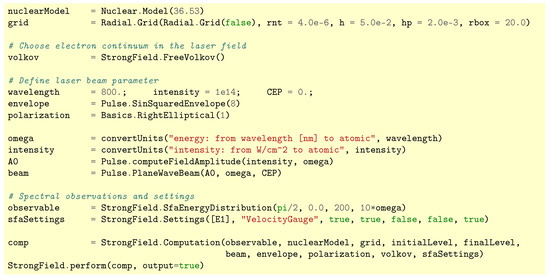
Figure 4.
Julia input for generating the black-solid ATI spectrum in the left panel of Figure 5 for a krypton target, if irradiated by an cycle sin laser pulse with a central wavelength of nm and intensity W/cm. The laser pulse is right-circularly polarized and has a carrier–envelope phase . This input describes the complete strong-field computation, but where the ground and the final levels of krypton are assumed to be generated before by the Jac toolbox. Although no attempt is made to explain this input in all detail, this figure nicely demonstrates how readily Jac can be utilized to generate rather different spectra and distributions. See text for further explanations.
In the input above, we finally also specify as observable an SfaEnergyDistribution(), and which is to be calculated for and (i.e., along the x-axis), and for 200-electron energies in the interval eV. All this input together determines the (strong-field) computation comp::StrongField.Computation and can be readily adopted to many other experimental scenarios. All that is needed in Jac is to perform(comp, output=true) this computation, and where the optional parameter output=true just tells Jac to return the calculated data (amplitudes) to the user for printing and post-processing.
Figure 5 displays the photoelectron energy spectra, emitted along the x-axis, for a krypton target and a right-circularly polarized laser pulse. The left panel shows the spectra as obtained for a computed with a hydrogenic initial wave function with adopted ionization potential and for a plane-wave Volkov continuum (black-solid curve) as well as a Coulomb–Volkov continuum (red dashed curve). On the right panel, in contrast, the spectra are computed for an initial orbital of neutral krypton and a plane-wave Volkov continuum (black-solid curve), a Coulomb–Volkov continuum (red-dashed curve) as well as a distorted-Volkov continuum (blue-dotted curve). In all these computations, a right-circularly polarized pulse of wavelength nm, intensity W/cm, carrier–envelope phase and with just cycles has been utilized.
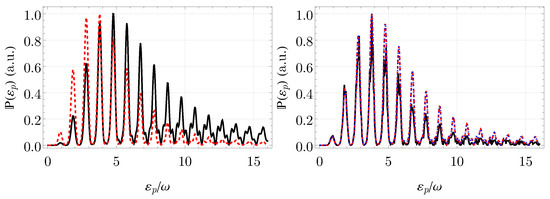
Figure 5.
Photoelectron energy spectra, emitted along the x-axis within the polarization plane, for a neutral krypton target and a right-circularly polarized laser pulse. The left panel shows the spectra as computed with a hydrogenic initial wave function with adopted ionization potential and for a plane-wave Volkov continuum (black-solid curve) as well as a Coulomb–Volkov continuum (red-dashed curve). On the right panel, in contrast, the spectra are computed for an initial orbital of neutral krypton and a plane-wave Volkov continuum (black-solid curve), a Coulomb–Volkov continuum (red-dashed curve) as well as a distorted-Volkov continuum (blue-dotted curve). In all these computations, a right-circularly polarized pulse of wavelength nm, intensity W/cm, carrier–envelope phase and with cycles has been utilized.
Input quite similar to Figure 4 can be employed also for studying the angle and momentum distributions of photoelectrons for different laser pulses and targets. While no further input data will be shown below, we refer the reader for details to the User Guide and the online documentation of the Jac program. Moreover, rather moderate changes to this input will be sufficient in the future to expand the StrongField module to other gauges, amplitudes or many-electron features. While such an expansion of the code indeed appears straightforward, major effort will still be needed for its implementation and testing.
3.2. Photoelectron Angular Distribution for Elliptically-Polarized Laser Pulses
In the electric-dipole (E1) approximation, the angular distribution of the photoelectrons is restricted to the polarization plane and just reflects at fixed photoelectron energy the ionization probability in Equation (1) for different azimuthal angles . If, moreover, the laser field dominates the electron dynamics in the continuum, the observed photoelectron angular distribution (PAD) should also reflect the symmetry of the vector potential of the laser beam. In practice, however, a Coulomb asymmetry in the PAD was (first) observed by Goreslavski et al. [33] in the ATI of xenon gas targets and, since then, has been found to be a valuable testbed for improving theory. For lithium, argon and xenon, for example, the SFA theory was shown to reproduce this asymmetry, if a target-specific initial orbital function is chosen along with a distorted-Volkov continuum for the active electron [34].
Figure 6 displays different photoelectron angular distributions in the polarization plane () for a krypton target. Angular distributions are shown for elliptically-polarized laser pulses with (left panel) and (right panel) at fixed photoelectron energy according to the third ATI peak in Figure 5. Different approximations are compared for these angular distributions: a hydrogenic initial orbital together with a plane-wave Volkov continuum (black-solid curves); a self-consistent initial orbital of neutral krypton together with a Coulomb–Volkov continuum (red long-dashed curves); the same initial orbital but together with a distorted-Volkov continuum (blue-dashed curves). All these distributions are normalized on their maximum, while all other laser parameters are the same as in Figure 5. Indeed, a self-consistent orbital of neutral krypton together with a Coulomb–Volkov continuum (red long-dashed curves) leads to a clear rotation of the PAD as mentioned above. Moreover, the PAD no longer exhibits an inversion symmetry with regard to the origin because of the short duration of the laser pulse. If, in addition, the Coulomb–Volkov continuum is replaced by an distorted-Volkov continuum (blue-dashed curves), and which accounts for an outgoing electron in the potential of the Kr photoion, the rotation angle still changes rather remarkably. In Ref. [19], it was shown that such a distorted-Volkov continuum (often) leads for different targets to better agreement with experiment.
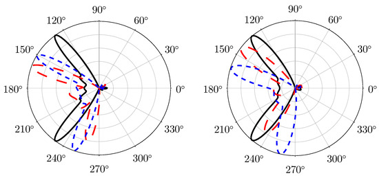
Figure 6.
Photoelectron angular distributions in the polarization plane () for a krypton target. Angular distributions are shown for elliptically-polarized laser beams with (left panel) and (right panel) at fixed photoelectron energy according to the third ATI peak in Figure 5. Different approximations are compared for these angular distributions: a hydrogenic initial orbital together with a plane-wave Volkov continuum (black-solid curves); a self-consistent initial orbital of neutral krypton together with a Coulomb–Volkov continuum (red long-dashed curves); the same initial orbital but together with a distorted-Volkov continuum (blue-dashed curves). All distributions are normalized on their maximum, while all other laser parameters are the same as in Figure 5.
3.3. Photoelectron Momentum Distribution for Few-Cycle Laser Pulses
Theoretical photoelectron momentum distributions (PMD) have been calculated in the literature by means of quite different methods, and by making use of even a larger number of case-specific modifications to these methods. Generally, the experimentally observed symmetries of the PMD cannot be explained so readily by just applying a plane-wave Volkov continuum [33], but can be improved further if the Coulomb potential of the residual ion is taken into account. In our implementation of the SFA direct amplitude, this is achieved by replacing the plane-wave Volkov continuum by either Coulomb–Volkov or distorted-Volkov states. For the low-energy photoelectrons with (say) , the ionization probability is then often enhanced by up to an order of magnitude, if the ionic charge just increases from to 1. This has been explained by the attractive Coulomb potential of the residual ion that pulls the electron back to the ion and hence reduces its kinetic energy. The low-energy part of the ATI spectra can be further improved by adding a short-range potential to the (long-range) Coulomb potential and by making use of distorted-Volkov states.
Figure 7 shows the photoelectron momentum distributions in the polarization plane () for the strong-field ionization of a krypton target. Momentum distributions are shown for circularly-polarized laser beams with three different CEP phases: (left panel), (middle panel) and (right panel) and by applying a self-consistent initial orbital of neutral krypton together with a plane-wave Volkov continuum. All further laser parameters are the same as in Figure 5. Obviously, the PMD in this figure exhibits a (very) clear rotation since the photoelectrons are preferably emitted in the polarization plane along the maximum of the vector potential [6], and which changes with the carrier envelope phase . It will be interesting to explain with Jac in future work how the Coulomb asymmetry and the CEP dependence act together upon the angular or momentum distributions, and, especially of the initial-bound and distorted-Volkov continuum states of different atomic targets, are taken properly into account. In these studies, both the Coulomb and short-range interactions can be easily incorporated into the continuum by just replacing the radial wave functions of the active electron.
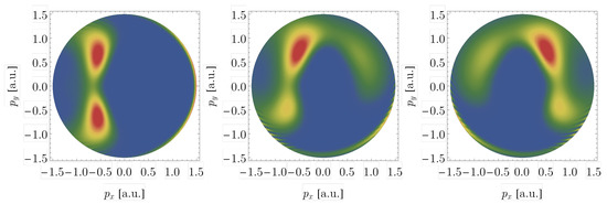
Figure 7.
Photoelectron momentum distributions in the polarization plane () for a krypton target. Momentum distributions are shown for circularly-polarized laser beams with three different CEP phases: (left panel), (middle panel) and (right panel) and by applying a self-consistent initial orbital of neutral krypton together with a plane-wave Volkov continuum. All further laser parameters are the same as in Figure 5.
4. Conclusions and Outlook
Up to the present, the SFA has been found as perhaps the most powerful method for predicting or analyzing the electron dynamics in strong-field ionization. Often, this approximation helps describe features in the observed electron distributions even quantitatively, if the initial-bound and final-continuum states of the photoelectron are well adopted to the target atoms, and if combined with a proper parameterization of the laser field. With the present implementation of the direct SFA amplitude into the Jac toolbox, this method can now be applied to different targets and strong-field scenarios. In particular, the implementation of the SFA in the partial-wave representation enables us to readily control (and replace) the wave functions and various details about the laser–electron interaction. It also enables us to extend this implementation for incorporating further interactions and mechanisms into the modeling.
Detailed calculations are performed for a krypton target as well as for different ATI spectra and PMD. These examples clearly show how the target potential affects the photoelectrons on their way to the detector and, hence, all the observed spectra. In particular, we have demonstrated how the electronic structure of the atomic targets can be taken into account in the representation of the active electron and how the dynamics of the outgoing electron can be readily controlled by applying different approximations for the Volkov continuum. Moreover, the use of partial waves and spherical tensor operators facilitates a simpler comparison of different pulse shapes and how they influence the observed ATI spectra and PMD.
Several extensions to the SFA are still desirable and appear feasible within a framework, which is based on a partial-wave representation of the associated strong-field amplitudes. While further effort will be needed to decompose these amplitudes into a form, suitable for computations, a few useful extensions concern:
- Non-dipole interactions: For spatially-structured light fields, non-dipole contributions to the Volkov continuum usually arise from the spatially dependent Volkov phase [35,36,37], and which need first to be expressed into a partial-wave representation in order to become applicable within Jac. These non-dipole terms beyond the widely used E1 approximation capture the combined-electric and magnetic-fields upon the electron dynamics [38,39]. Their implementation into the Jac toolbox will help predict the energy and momentum shifts at long wavelengths of the driving fields.
- Coupling of the radiation field: Apart from the (commonly applied) velocity gauge, the direct amplitude can be also implemented in length gauge. This leads to more complicated pulse-shape integrals that also comprise the reduced matrix elements of the momentum operator, since the kinetic momentum then needs to be replaced by the (time-dependent) canonical momentum. While such an implementation requires further work, the direct SFA amplitude in length gauge was shown to provide more accurate results for the ionization of non-spherical electrons [40].
- Rescattering amplitude: For laser pulses with proper polarization, the electrons are known to be partly rescattered by the photoion, which then leads to processes, such as high-order ATI, the non-sequential double ionization, or even to high-order harmonics beyond the well-known cut-off law [41]. A partial-wave representation of the rescattering amplitude (2) is currently worked out and can be applied to account for realistic rescattering potentials.
- High-harmonic generation: Similar to the rescattering ATI amplitude above, a recombination amplitude needs to be computed in order to obtain the dipole moment of emitted high-harmonic radiation. For modeling HHG, again, we expect to benefit from a re-formulation of the dipole amplitude in terms of partial waves and from including realistic initial and continuum orbitals [42,43].
- Role of bound states: The coupling of the ground and continuum states to other excited (bound) states has been analyzed in the literature for just a (very) few selected HHG spectra [44]. A partial-wave representation of the SFA amplitudes facilitates the coupling to excited states of the target and may help explain the formation and influence of (autoionizing) resonances in the HHG plateau.
- Many-electron effects: A consequent partial-wave decomposition of all strong-field amplitudes enables one to incorporate many-electron contributions beyond a (spherical) short-range potential into the formalism. Apart from the self-consistent field and the mixing of important configurations, this also refers to the treatment of the multipole contributions (higher than E1), if the corresponding many-electron matrix elements are utilized [45,46].
- Nonsequential double ionization (NSDI): When the photoelectron returns to the photoion, the electron can scatter inelastically under the ionization of a second electron. Theoretically, the NSDI is typically described semi-classically by using excitation and/or ionization cross sections for the second (ionizing) step of the process [47,48]. A partial-wave representation of all associated quantum SFA amplitude facilitates a coherent treatment of this nonlinear ionization process.
For all these desirable extensions, the partial-wave representation of the SFA [15], and its implementation in Jac provides a straight and conceivably the best way to advance theory and the light–atom interaction in strong fields.
Author Contributions
Methodology, S.F. and B.B.; software, S.F. and B.B.; writing—review and editing, S.F. and B.B. All authors have read and agreed to the published version of the manuscript.
Funding
This work has been funded by the Deutsche Forschungsgemeinschaft (DFG, German Research Foundation)—440556973.
Institutional Review Board Statement
Not applicable.
Informed Consent Statement
Not applicable.
Data Availability Statement
Not applicable.
Conflicts of Interest
The authors declare no conflict of interest.
References
- Agostini, P.; Fabre, F.; Mainfray, G.; Petite, G.; Rahman, N.K. Free-free transitions following six-photon ionization of xenon atoms. Phys. Rev. Lett. 1979, 42, 1127. [Google Scholar] [CrossRef]
- Paulus, G.G.; Nicklich, W.; Huale, X.; Lambropoulos, P.; Walther, H. Plateau in above threshold ionization spectra. Phys. Rev. Lett. 1994, 72, 2851. [Google Scholar] [CrossRef] [PubMed]
- McPherson, A.; Gibson, G.; Jara, H.; Johann, U.; Luk, T.S.; McIntyre, I.A.; Boyer, K.; Rhodes, C.K. Studies of multiphoton production of vacuum-ultraviolet radiation in the rare gas. J. Opt. Soc. Am. B 1987, 4, 595–601. [Google Scholar] [CrossRef]
- Ferray, M.; L’Huillier, A.; Li, X.F.; Lompre, L.A.; Mainfray, G.; Manus, C. Multiple-harmonic conversion of 1064 nm radiation in rare gases. J. Phys. B 1988, 21, L31. [Google Scholar] [CrossRef]
- L’Huillier, A.; Lompre, L.A.; Mainfray, G.; Manus, C. Multiply charged ions formed by multiphoton absorption processes in the continuum. Phys. Rev. Lett. 1982, 48, 1814. [Google Scholar] [CrossRef]
- Milosevic, D.B.; Paulus, G.G.; Bauer, D.; Becker, W. Above-threshold ionization by few-cycle pulses. J. Phys. B 2006, 39, R203. [Google Scholar] [CrossRef]
- Böning, B.; Abele, P.; Paufler, W.; Fritzsche, S. Above-threshold ionization of Ba+ with realistic initial states in the strong-field approximation. J. Phys. B 2021, 54, 025602. [Google Scholar] [CrossRef]
- Ivanov, I.A.; Kheifets, A.S. Angle-dependent time delay in two-color XUV+IR photoemission of He and Ne. Phys. Rev. A 2017, 96, 013408. [Google Scholar] [CrossRef]
- Keldysh, L.V. Ionization in the field of a strong electromagnetic wave. Sov. Phys. JETP 1964, 20, 1307. [Google Scholar]
- Faisal, F.H.M. Multiple absorption of laser photons by atoms. J. Phys. B At. Mol. Phys. 1973, 6, L89. [Google Scholar] [CrossRef]
- Reiss, H.R. Effect of an intense electromagnetic field on a weakly bound system. Phys. Rev. A 1980, 22, 1786. [Google Scholar] [CrossRef]
- Ivanov, M.Y.; Spanner, M.; Smirnova, O. Anatomy of strong field ionization. J. Mod. Opt. 2005, 52, 165–184. [Google Scholar] [CrossRef]
- Amini, K.; Biegert, J.; Calegari, F.; Chacón, A.; Ciappina, M.F.; Dauphin, A.; Efimov, D.K.; de Morisson Faria, C.F.; Giergiel, K.; Gniewek, P.L.; et al. Symphony on strong field approximation. Rep. Progr. Phys. 2019, 82, 116001. [Google Scholar] [CrossRef] [Green Version]
- Kheifets, A. Revealing the target electronic structure with under-threshold RABBITT. Atoms 2021, 9, 66. [Google Scholar] [CrossRef]
- Böning, B.; Fritzsche, S. Partial-wave representation of the strong-field approximation. Phys. Rev. A 2020, 102, 053108. [Google Scholar] [CrossRef]
- Fritzsche, S. A fresh computational approach to atomic structures, processes and cascades. Comp. Phys. Commun. 2019, 240, 1–14. [Google Scholar] [CrossRef]
- Schippers, S.; Martins, M.; Beerwerth, R.; Bari, S.; Holste, K.; Schubert, K.; Viefhaus, J.; Savin, D.W.; Fritzsche, S.; Müller, A. Near L-edge single and multiple photoionization of singly charged iron ions. Astrophys. J. 2017, 849, 5. [Google Scholar] [CrossRef] [Green Version]
- Fritzsche, S. Level structure and properties of open f-shell elements. Atoms 2022, 10, 7. [Google Scholar] [CrossRef]
- Böning, B.; Fritzsche, S. Partial-wave representation of the strong-field approximation. Atomic states and Coulomb asymmetry. Phys. Rev. A 2022. submitted. [Google Scholar]
- Faisal, F.H.M. Strong-field S-matrix theory with final-state Coulomb interaction in all orders. Phys. Rev. A 2016, 94, 031401. [Google Scholar] [CrossRef] [Green Version]
- Milosevic, D.B.; Becker, W. Atom-Volkov strong-field approximation for above-threshold ionization. Phys. Rev. A 2019, 99, 043411. [Google Scholar] [CrossRef]
- Schippers, S.; Beerwerth, R.; Ábrók, L.; Bari, S.; Buhr, T.; Martins, M.; Ricz, S.; Viefhaus, J.; Fritzsche, S.; Müller, A. Prominent role of multielectron processes in K-shell double and triple photodetachment of oxygen anions. Phys. Rev. A 2016, 94, 041401(R). [Google Scholar] [CrossRef] [Green Version]
- Beerwerth, R.; Buhr, T.; Perry-Sassmannshausen, A.; Stock, S.O.; Bari, S.; Holste, K.; Kilcoyne, A.D.; Reinwardt, S.; Ricz, S.; Savin, D.W.; et al. Near L-edge single and multiple photoionization of triply charged iron ions. Astrophys. J. 2019, 887, 189. [Google Scholar] [CrossRef] [Green Version]
- Perry-Sassmannshausen, A.; Buhr, T.; Borovik, A., Jr.; Martins, M.; Reinwardt, S.; Ricz, S.; Stock, S.O.; Trinter, F.; Müller, A.; Fritzsche, S.; et al. Multiple photodetachment of carbon anions via single and double core-hole creation. Phys. Rev. Lett. 2020, 124, 083203. [Google Scholar] [CrossRef] [Green Version]
- Fritzsche, S. JAC: User Guide, Compendium & Theoretical Background. Unpublished. Available online: https://github.com/OpenJAC/JAC.jl (accessed on 10 February 2022).
- Julia 1.7 Documentation. Available online: https://docs.julialang.org/ (accessed on 10 May 2022).
- Bezanson, J.; Chen, J.; Chung, B.; Karpinski, S.; Shah, V.B.; Vitek, J.; Zoubritzky, L. Julia: Dynamism and performance reconciled by design. Proc. ACM Program. Lang. 2018, 2, 120. [Google Scholar] [CrossRef] [Green Version]
- Fritzsche, S.; Fricke, B.; Sepp, W.D. Reduced L1 level-width and Coster-Kronig yields by relaxation and continuum interactions in atomic zinc. Phys. Rev. A 1992, 45, 1465. [Google Scholar] [CrossRef] [Green Version]
- Gaigalas, G.; Fritzsche, S. Angular coefficients for symmetry-adapted configuration states in jj-coupling. Comput. Phys. Commun. 2021, 267, 108086. [Google Scholar] [CrossRef]
- Fritzsche, S.; Palmeri, P.; Schippers, S. Atomic cascade computations. Symmetry 2021, 13, 520. [Google Scholar] [CrossRef]
- Fritzsche, S. Dielectronic recombination strengths and plasma rate coefficients of multiply-charged ions. Astron. Astrophys. 2021, 656, 163. [Google Scholar] [CrossRef]
- Julia Comes with a Full-Featured Interactive and Command-Line REPL (Read-Eval-print Loop) that Is Built into the Executable of the Language. Available online: https://docs.julialang.org/en/v1/stdlib/REPL/ (accessed on 10 May 2022).
- Goreslavski, S.P.; Paulus, G.G.; Popruzhenko, S.V.; Shvetsov-Shilovski, N.I. Coulomb asymmetry in above-threshold ionization. Phys. Rev. Lett. 2004, 93, 233002. [Google Scholar] [CrossRef] [Green Version]
- Böning, B.; Fritzsche, S. Steering the longitudinal photoelectron momentum in above-threshold ionization with not quite collinear laser beams. Phys. Rev. A 2022. accepted. [Google Scholar]
- Böning, B.; Paufler, W.; Fritzsche, S. Nondipole strong-field approximation for spatially structured laser fields. Phys. Rev. A 2019, 99, 053404. [Google Scholar] [CrossRef]
- Wolkow, D.M. Über eine Klasse von Lösungen der Diracschen Gleichung. Z. Phys. 1935, 94, 250–260. [Google Scholar] [CrossRef]
- Rosenberg, L.; Zhou, F. Generalized Volkov wave functions: Application to laser-assisted scattering. Phys. Rev. A 1993, 47, 2146. [Google Scholar] [CrossRef]
- Böning, B.; Fritzsche, S. Above-threshold ionization driven by Gaussian laser beams: Beyond the electric dipole approximation. J. Phys. B At. Mol. Phys. 2021, 54, 144002. [Google Scholar] [CrossRef]
- Böning, B.; Paufler, W.; Fritzsche, S. Polarization-dependent high-intensity Kapitza-Dirac effect in strong laser fields. Phys. Rev. A 2020, 101, 031401(R). [Google Scholar]
- Bauer, D.; Milosevic, D.B.; Becker, W. Strong-field approximation for intense-laser–atom processes: The choice of gauge. Phys. Rev. A 2005, 72, 023415. [Google Scholar] [CrossRef] [Green Version]
- Dionissopoulou, S.; Lyras, A.; Mercouris, T.; Nicolaides, C.A. High-order above threshold ionization spectrum of hydrogen and photoelectron angular distributions. J. Phys. B At. Mol. Phys. 1995, 28, L109. [Google Scholar] [CrossRef]
- Paufler, W.; Böning, B.; Fritzsche, S. High harmonic generation with Laguerre-Gaussian beams. J. Opt. 2019, 21, 094001. [Google Scholar] [CrossRef]
- Paufler, W.; Böning, B.; Fritzsche, S. Tailored orbital angular momentum by high-harmonic generation from counterrotating bi-circular Laguerre-Gaussian beams. Phys. Rev. A 2018, 98, 011401(R). [Google Scholar]
- Klaiber, M.; Hatsagortsyan, K.Z.; Keitel, C.H. Sub-barrier pathways to Freeman resonances. Phys. Rev. A 2020, 102, 053105. [Google Scholar] [CrossRef]
- Johnson, W.R. Atomic Structure Theory: Lectures on Atomic Physics; Springer: Berlin/Heidelberg, Germany, 2007. [Google Scholar]
- Fritzsche, S. The Ratip program for relativistic calculations of atomic transition, ionization and recombination properties. Comp. Phys. Commun. 2012, 183, 1525–1559. [Google Scholar] [CrossRef]
- Chen, Z.; Wang, Y.; Morishita, T.; Hao, X.; Chen, J.; Zatsarinny, O.; Bartschat, K. Revisiting the recollisional excitation-tunneling process in strong-field nonsequential double ionization of helium. Phys. Rev. A 2019, 100, 023405. [Google Scholar] [CrossRef]
- Liu, F.; Chen, Z.; Morishita, T.; Bartschat, K.; Böning, B.; Fritzsche, S. Single-cycle versus multicycle nonsequential double ionization of argon. Phys. Rev. A 2021, 104, 013105. [Google Scholar] [CrossRef]
Publisher’s Note: MDPI stays neutral with regard to jurisdictional claims in published maps and institutional affiliations. |
© 2022 by the authors. Licensee MDPI, Basel, Switzerland. This article is an open access article distributed under the terms and conditions of the Creative Commons Attribution (CC BY) license (https://creativecommons.org/licenses/by/4.0/).