Analytical Approximations to Charged Black Hole Solutions in Einstein–Maxwell–Weyl Gravity

Abstract

The homotopy analysis method (HAM) is a useful method to derive analytical approximate solutions of black holes in modified gravity theories. In this paper, we study the Einstein–Weyl gravity coupled with Maxwell field and obtain analytical approximation solutions for charged black holes by using the HAM. It is found that the analytical approximate solutions are sufficiently accurate in the entire spacetime outside the black hole’s event horizon and also consistent with numerical ones for charged black holes in the Einstein–Maxwell–Weyl gravity.

1. Introduction

It is widely recognized that the theory of general relativity (GR) does not qualify as a renormalizable quantum field theory within the framework of effective field theory. Therefore, to achieve the ultimate goal of unifying GR with quantum theory, it is imperative to explore alternative theories that go beyond GR. A possible attempt to solve the problem of the non-renormalizability of GR is to include higher-order corrections that become important at higher energy. Some years ago, Stelle [1] proposed to add all possible quadratic curvature invariants to the usual Einstein–Hilbert action and then obtained a theory of quantum gravity free of ultraviolet divergences but as early recognized [2], albeit at the price of introducing ghost-like modes. In four-dimensional spacetime, the most comprehensive theory that includes second-order derivative terms in the curvature can be expressed as follows [3,4]

$$\mathcal{I}=\int d^{4}x\sqrt{-g}\left(\gamma R-\alpha C_{\mu \rho \nu \sigma }{C}^{\mu \rho \nu \sigma }+\beta R^2\right),$$

(1)

where the parameters $\alpha$, $\beta$, and $\gamma$ are constants and $C_{\mu \rho \nu \sigma }$ is the Weyl tensor. In addition, black holes are fundamental objects in theories of gravity and serve as powerful tools for studying the intricate global aspects of the theory. Subsequently, Lü et al. [4,5] derived numerical solutions of non-Schwarzschild black holes (NSBH) in the Einstein–Weyl gravity [Equation (1)] by considering the disappearance of the Ricci scalar for any static spherically symmetric black hole solution ($R=0$). Actually, the no-go theorem also implies that the Ricci scalar R must be zero for a black hole in the case of pure gravity or with a traceless matter stress tensor. In Refs. [4,5], they further investigated some thermodynamic properties of NSBH and discovered several remarkable features: (1) the NSBH can have positive and negative masses; (2) as the coupling constant $\alpha$ approaches its extreme value, the black hole tends towards a massless state while maintaining a nonzero radius. Recently, Held et al. [6] discussed the linear stability of these two branches of black hole solutions. In addition, charged black holes in the Einstein–Weyl gravity coupled with (nonlinear) Maxwell field were constructed in Refs. [7,8] and our previous works [9,10], where two sets of numerical solutions were obtained: the charged generalization of the Schwarzschild solution and the charged generalization of the non-Schwarzschild solution. The analysis of quasinormal modes of the non-Schwarzschild and charged black holes was performed in the Einstein–Weyl gravity [11,12,13], where the linear relation between quasinormal mode frequencies and the parameter was recovered. Later, the black holes with massive scalar hair were obtained in Ref. [14], where they discussed the effects of the scalar field on the black hole structure. Recently, some novel solutions of black holes were also studied in the Einstein–Weyl gravity [15,16], including the phase diagram of Einstein–Weyl gravity [17].

However, the numerical solutions for non-Schwarzschild black holes have limitations to providing a clear understanding of the dependence of the metric on physical parameters, as they are obtained at fixed parameter values and displayed as curves in figures rather than explicit expressions. This makes it difficult for researchers to use these solutions in their work without recalculating them. Fortunately, there are general methods available for parametrizing black hole spacetimes, such as the continued fractions method (CFM) [18,19] and the homotopy analysis method (HAM) [20,21,22]. In this paper, we focus on the HAM. It is considered as a very useful method for obtaining analytical approximate solutions for various nonlinear differential equations, including those arising in different areas of science and engineering. Despite its widespread use in other fields, the HAM has been limited in the fields of general relativity and gravitation. Recently, we constructed analytical approximation solutions of scalarized AdS black holes in Einstein-scalar-Gauss–Bonnet gravity by using HAM [23]. Moreover, this HAM has been adopted to derive the analytical approximation solutions of non-Schwarzschild black holes in the Einstein–Weyl gravity [24] and analytic approximate solutions of hairy black holes in Einstein–Weyl-scalar gravity [25] as well as for the Regge–Wheeler equations under metric perturbations on the Schwarzschild spacetime [26]. The above works inspire us to continue exploring the application of homotopy analysis in modified gravity theory. In this work, we wish to apply the HAM to obtain analytical approximation solutions of charged black holes in the Einstein–Maxwell–Weyl gravity.

The plan of the paper is as follows. In Section 2, we review the Einstein–Weyl gravity coupled with Maxwell field and present the numerical solutions for a charged black hole in the Einstein–Maxwell–Weyl gravity. Section 3 is devoted to deriving the analytical approximation solutions by using the HAM method, where two solutions are accurate in the whole space outside the event horizon. The paper ends with a discussion of the results obtained in Section 4.

2. The Einstein–Maxwell–Weyl Gravity

The action of Einstein–Weyl gravity in the presence of Maxwell field is given by [7]

$$\mathcal{I}=\int d^{4}x\sqrt{-g}\left(\gamma R-\alpha C_{\mu \rho \nu \sigma }{C}^{\mu \rho \nu \sigma }+\beta R^2-\kappa F_{\mu \nu }{F}^{\mu \nu }\right),$$

(2)

where the parameters $\gamma$, $\alpha$, $\beta$, and $\kappa$ are coupling constants, $F_{\mu \nu }={\nabla }_{\mu }{A}_{\nu }-{\nabla }_{\nu }{A}_{\mu }$ is the electromagnetic tensor, and $C_{\mu \rho \nu \sigma }$ is the Weyl tensor. Since resulting tensors in the equations of motion that come from the Weyl and Maxwell energy momentum tensors are traceless, a charged black hole solution in this theory should not need the contribution from the $\beta R^2$ term [7]. Taking $\beta =0$ and $\gamma =1$, the corresponding field equations are obtained as

$$\begin{array}{}\mathrm{(3)}& R_{\mu \nu }-\frac{1}{2}{g}_{\mu \nu }R-4\alpha B_{\mu \nu }-2\kappa T_{\mu \nu }=0,\hfill \mathrm{(4)}& {\nabla }_{\mu }{F}^{\mu \nu }=0,\hfill \end{array}$$

where the trace-free Bach tensor $B_{\mu \nu }$ and energy–momentum tensor of electromagnetic field $T_{\mu \nu }$ are defined as

$$\begin{array}{c}\hfill B_{\mu \nu }=\left({\nabla }^{\rho }{\nabla }^{\sigma }+\frac{1}{2}{R}^{\rho \sigma }\right)C_{\mu \rho \nu \sigma },\\ \hfill T_{\mu \nu }=F_{\alpha \mu }{F^{\alpha }}_{\nu }-\frac{1}{4}{g}_{\mu \nu }{F}_{\alpha \beta }{F}^{\alpha \beta }.\end{array}$$

(5)

Considering the static and spherical symmetry metric ansatz,

$$\begin{array}{c}\hfill d{s}^2=-h\left(r\right)d{t}^2+\frac{1}{f\left(r\right)}d{r}^2+r^2({d\theta }^2+{sin}^2\theta {d\varphi }^2),\end{array}$$

(6)

and substituting the metric ansatz into the field Equations (3) and (4), we obtain three independent equations

$$\begin{array}{ccc}\hfill h^{″}\left(r\right)=& & \frac{4h{\left(r\right)}^2\left(1-r{f}^{\prime }\left(r\right)-f\left(r\right)\right)-rh\left(r\right)\left(r{f}^{\prime }\left(r\right)+4f\left(r\right)\right)h^{\prime }\left(r\right)+r^{2}f\left(r\right)h^{\prime }{\left(r\right)}^2}{2r^{2}f\left(r\right)h\left(r\right)}\hfill \\ \hfill f^{″}\left(r\right)=& & \frac{h\left(r\right)-f\left(r\right)h\left(r\right)-rf\left(r\right)h^{\prime }\left(r\right)}{\alpha f\left(r\right)\left[2h\left(r\right)-r{h}^{\prime }\left(r\right)\right]}\hfill \\ & & -\frac{h\left(r\right)\left[3r^2{f}^{\prime }{\left(r\right)}^2+12rf\left(r\right)f^{\prime }\left(r\right)-4r{f}^{\prime }\left(r\right)+12f{\left(r\right)}^2-8f\left(r\right)\right]}{2r^{2}f\left(r\right)\left[r{h}^{\prime }\left(r\right)-2h\left(r\right)\right]}\hfill \\ & & +\frac{\kappa Q_0^{2}h\left(r\right)}{\alpha r^{2}f\left(r\right)\left[r{h}^{\prime }\left(r\right)-2h\left(r\right)\right]}\hfill \\ & & +\frac{f\left(r\right)\left[r^2{h}^{\prime }{\left(r\right)}^2-rh\left(r\right)h^{\prime }\left(r\right)-2h{\left(r\right)}^2\right]-rh\left(r\right)f^{\prime }\left(r\right)\left[r{h}^{\prime }\left(r\right)+4h\left(r\right)\right]}{2r^{2}h{\left(r\right)}^2}\hfill \\ \hfill A_t^{\prime }\left(r\right)=& & -\frac{Q_0}{r^2}\sqrt{\frac{h\left(r\right)}{f\left(r\right)}},\hfill \end{array}$$

(7)

where the prime (${}^{\prime }$) denotes differentiation with respect to r and $Q_0$ denotes electric charge. If $Q_0\to 0$, the equations of motion (7) reduce to those found in Refs. [4,5,19] and recover the same solutions: the Schwarzschild black holes (SBH) and the non-Schwarzschild black holes (NSBH).

Now we derive the numerical solutions of charged black holes. Here, we suppose that the spacetime has only one horizon to make easier the expansion of $f\left(r\right)$, $h\left(r\right)$, and $A_t\left(r\right)$ around the event horizon $r_0$

$$\begin{array}{}\mathrm{(8)}& h\left(r\right)=c[\left(r-r_0\right)+h_2{\left(r-r_0\right)}^2+h_3{\left(r-r_0\right)}^3+\dots ],\hfill \mathrm{(9)}& f\left(r\right)=f_1\left(r-r_0\right)+f_2{\left(r-r_0\right)}^2+f_3{\left(r-r_0\right)}^3+\dots ,\hfill \mathrm{(10)}& A_t\left(r\right)=A_{t0}+A_{t1}\left(r-r_0\right)+A_{t2}{\left(r-r_0\right)}^2+\dots ,\hfill \end{array}$$

where $h_i$, $f_i$, and $A_{ti}$ are constant coefficients of the expansions and c is the arbitrary scaling factor, which we choose such that t is the time coordinate of a remote observer, i.e.,

$$\begin{array}{c}\hfill \underset{r\to \infty }{lim}h\left(r\right)=1.\end{array}$$

(11)

Moreover, the expansion parameter.

Substituting the above expansions (8)–(10) into field Equation (7), arbitrary coefficients $h_j$, $f_j$, and $A_{ti}$ with $j\ge 2$ can be expressed in terms of $f_1$, for example, $h_2$, $f_2$, $A_{t2}$, and $A_{t1}$ are expressed as

$$\begin{array}{ccc}& & h_2=\frac{1-2f_1{r}_0}{r_0^2}-\frac{r_0^2-f_1{r}_0^3-\kappa Q_0^2}{8\alpha f_1{r}_0^3},\hfill \\ & & f_2=\frac{1-2f_1{r}_0}{r_0^2}-\frac{3\left(r_0^2-f_1{r}_0^3-\kappa Q_0^2\right)}{8\alpha f_1{r}_0^3},\hfill \\ & & A_{t1}=-\frac{Q_0}{r_0^2},A_{t2}=\frac{Q_0}{r_0^3}+\frac{Q_0\left(r_0^3{f}_1+\kappa Q_0^2-r_0^2\right)}{8\alpha r_0^5{f}_1^2}.\hfill \end{array}$$

(12)

On the other hand, at the radial infinity $(r\to \infty )$, the metric functions and vector potential can be expanded in power series, this time in terms of $1/r$. Demanding that the metric components reduces to those of the asymptotically flat Minkowski spacetime

$$\begin{array}{ccc}& & h\left(r\right)=1-\frac{2M}{r}+\dots ,f\left(r\right)=1-\frac{2M}{r}+\dots ,\hfill \\ & & A_t\left(r\right)={\mathrm{\Phi }}_{\infty }+\frac{Q_0}{r}+\dots .\hfill \end{array}$$

(13)

Taking $\alpha =\frac{1}{2}$ and $\kappa =1$, we assume the initial values of the parameters $Q_0$ and $f_1$ at a radius $r_i=r_0+\frac{1}{1000}$ just outside the horizon $r_0$ and then use numerical routines in Mathematica^® to integrate the equations out to a large radius so that these interpolation functions of metric functions $h\left(r\right)$ and $f\left(r\right)$ and vector potential $A_t\left(r\right)$ satisfy the boundary condition (13). To ensure that $h\left(r\right)$ is asymptotically flat ${lim}_{r\to +\infty }h\left(r\right)=1$, the value of scaling parameter c equals to $0.3367$ for $Q_0=1$ and $r_0=2$, and $0.5521$ for $Q_0=1/2$ and $r_0=4/3$. In addition, the vector potential should satisfy the boundary

$$\begin{array}{c}\hfill \underset{r\to \infty }{lim}{A}_t\left(r\right)=0.\end{array}$$

(14)

For simplicity, we choose ${\mathrm{\Phi }}_{\infty }=0$. Then, we can obtain the values of $A_{t0}=0.4950$ and $0.3670$ for charged black holes with $Q_0=1$ and $Q_0=1/2$, respectively. The corresponding numerical solutions are plotted in Figure 1.

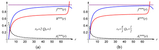
Figure 1. Numerical solutions of charged black holes for $h\left(r\right)$, $f\left(r\right)$, and $A_t\left(r\right)$ with different values of $r_0$ and $Q_0$. Here, $h\left(r\right)$ has been rescaled to approach $3/4$ to avoid overlap.

3. Analytically Approximate Solutions

In general, it is a difficult task to find exact solutions of nonlinear differential equations. In Refs. [21,22,27], the homotopy analysis method (HAM) was developed to obtain analytical approximate solutions to nonlinear differential equations. In this section, we will derive the analytical approximate solutions of metric functions and the electric potential function by using the HAM.

Consider an n-nonlinear differential equations system, where $y_i\left(t\right)$ is the solution of the nonlinear operator $N_i$ as a function of t

$$\begin{array}{c}\hfill N_i\left[y_i\left(t\right)\right]=0,i=1,2,\dots ,n,\end{array}$$

(15)

with unknown function $y_i\left(t\right)$ and a variable t. Then, the zero-order deformation equation can be written as

$$\begin{array}{c}\hfill (1-q)L[{\varphi }_i(t;q)-y_{i0}\left(t\right)]=q{h}_i{H}_i\left(t\right)N_i\left[{\varphi }_i(t;q)\right].\end{array}$$

(16)

The HAM constructs a topological homotopy for linear auxiliary operator L and nonlinear operator $N_i$. Introducing an embedding parameter $q\in [0,1]$, when q continuously changes from 0 to 1, the solution of the entire equation will also continuously change from the solution $y_{i0}\left(t\right)$ of our selected linear auxiliary operator L to the solution $y_i\left(t\right)$ of the nonlinear equation $N_i$. In order to control the convergence of the solution, an auxiliary function $H_i\left(t\right)$ and a convergence control parameter $h_i$ are also introduced into the homotopy Equation (16). By selecting the appropriate auxiliary function $H_i\left(t\right)$ and convergence control parameter $h_i$, the solution can converge more rapidly.

To decompose the nonlinear problem into a series of linear subproblems, now make Taylor expansions of ${\varphi }_i(t;q)$ with respect to q around $q=0$

$$\begin{array}{c}\hfill {\varphi }_i(t;q)=y_{i0}\left(t\right)+\sum _{m=1}^{\infty }{y}_{im}\left(t\right)q^m.\end{array}$$

(17)

where the coefficient $y_{im}\left(t\right)$ of the m-th order of q is

$$\begin{array}{c}\hfill y_{im}\left(t\right)=\frac{1}{m!}\frac{{\partial }^m{\varphi }_i(t;q)}{\partial q^m}.\end{array}$$

(18)

When $q=1$, it is the expansion of the solution of the nonlinear Equation (15)

$$\begin{array}{c}\hfill y_i\left(t\right)={\varphi }_i(t;1)=y_{i0}\left(t\right)+\sum _{m=1}^{\infty }{y}_{im}\left(t\right).\end{array}$$

(19)

By solving $y_{im}\left(t\right)$, the expansions of the solutions of the nonlinear equations can be found. To achieve this, the operation for the zero-order deformation Equation (16) will be as follows: First, substitute the expansion (17) into (16). Second, take the m-th derivative of q on both sides of (16). Third, after calculating the derivatives, set $q=0$. The so-called higher-order deformation equation (mth-order deformation equation) is obtained, which is summarized as

$$\begin{array}{c}\hfill L[y_{im}\left(t\right)-{\chi }_m{y}_{im-1}\left(t\right)]=h_i{H}_i\left(t\right)R_{im}\left(y_{im-1}\right),\end{array}$$

(20)

where the term $R_{im}$ on the right-hand side with respect to the nonlinear operator is

$$\begin{array}{c}\hfill R_{im}\left(y_{im-1}\right)=\frac{1}{(m-1)!}\frac{{\partial }^{m-1}{N}_i\left[{\sum }_{m=0}^{\infty }{y}_{im}\left(t\right)q^m\right]}{\partial q^{m-1}}{\mid }_{q=0}.\end{array}$$

(21)

The highest term on the right-hand side of Equation (21) can only reach up to the $y_{im-1}$ term. It is found that $y_{im}\left(t\right)$ is related to $y_{im-1}$, and it is possible to find $y_{im}\left(t\right)$ of arbitrary order based on this relation. The value of constant ${\chi }_m$ is

$$\begin{array}{c}\hfill {\chi }_m=\left\{\begin{array}{cc}\hfill 0& :m\le 1,\hfill \\ \hfill 1& :m>1.\hfill \end{array}\right.\end{array}$$

(22)

In the calculation, we take a finite order to ensure that the error is small enough, a finite M-order approximation

$$\begin{array}{c}\hfill y_i^M\left(t\right)=y_{i0}\left(t\right)+\sum _{m=1}^M{y}_{im}\left(t\right),\end{array}$$

(23)

the $y_i^M\left(t\right)$ are the M-th order approximate solutions of the original Equation (15).

The selection of linear auxiliary operator L, initial guess $y_{i0}\left(t\right)$, auxiliary function $H_i\left(t\right)$, and convergence control parameter $h_i$ has great freedom, making the homotopy analysis method highly adaptable to different nonlinear problems. However, precisely because there is a great deal of freedom in selecting these quantities, how to choose these quantities more appropriately still requires a theoretical basis, and related work can be found in [28,29].

Next, we will use the HAM to obtain analytical approximation solutions of charged black holes in the Einstein–Maxwell–Weyl gravity. In order to do this, we choose a coordinate transformation $z=1-\frac{r_0}{r}$, such that the region of $r\to \infty$ becomes a finite value $z=1$. Then, the field equations under this coordinate transformation become

$$h^{″}\left(z\right)-\frac{h^{\prime }{\left(z\right)}^2}{2h\left(z\right)}+\frac{f^{\prime }\left(z\right)h^{\prime }\left(z\right)}{2f\left(z\right)}+\frac{2h\left(z\right)\left[-(z-1)f^{\prime }\left(z\right)+f\left(z\right)-1\right]}{{(z-1)}^{2}f\left(z\right)}=0,$$

(24)

$$\begin{array}{ccc}& & f\left(z\right)f^{″}\left(z\right)\left[2\alpha {(z-1)}^{5}h{\left(z\right)}^2{h}^{\prime }\left(z\right)+4\alpha {(z-1)}^{4}h{\left(z\right)}^3\right]\hfill \\ & & +f^{\prime }\left(z\right)\{f\left(z\right)\left[\alpha {(z-1)}^{5}h\left(z\right)h^{\prime }{\left(z\right)}^2+2\alpha {(z-1)}^{4}h{\left(z\right)}^2{h}^{\prime }\left(z\right)+12\alpha {(z-1)}^{3}h{\left(z\right)}^3\right]\hfill \\ & & -4\alpha {(z-1)}^{3}h{\left(z\right)}^3\}-3\alpha {(z-1)}^{4}h{\left(z\right)}^3{f}^{\prime }{\left(z\right)}^2+f\left(z\right)\left[-2{r_0}^2(z-1)h{\left(z\right)}^2{h}^{\prime }\left(z\right)\right.\hfill \\ & & \left.+2{r_0}^{2}h{\left(z\right)}^3+8\alpha {(z-1)}^{2}h{\left(z\right)}^3\right]+f{\left(z\right)}^2\left[-\alpha {(z-1)}^5{h}^{\prime }{\left(z\right)}^3-3\alpha {(z-1)}^{4}h\left(z\right)h^{\prime }{\left(z\right)}^2\right.\hfill \\ & & \left.-8\alpha {(z-1)}^{2}h{\left(z\right)}^3\right]+2\kappa {Q_0}^2{(z-1)}^{2}h{\left(z\right)}^3-2{r_0}^{2}h{\left(z\right)}^3=0,\hfill \end{array}$$

(25)

$$\begin{array}{ccc}& & \frac{Q_0\sqrt{\frac{h\left(z\right)}{f\left(z\right)}}}{r_0}+A_t^{\prime }\left(z\right)=0,\hfill \end{array}$$

(26)

where the prime (${}^{\prime }$) denotes the differentiation of the function with respect to z and $r_0$ is the event horizon of the black hole. Notice that Maxwell Equation (26) is a linear one and (24) and (25) are second-order derivative equations with respect to $h\left(z\right)$ and $f\left(z\right)$. Therefore, we derive $h\left(z\right)$ and $f\left(z\right)$ by applying the HAM to the two nonlinear Equations (24) and (25), after then solving Equation (26) for $A_t\left(z\right)$.

In the homotopy equation, the auxiliary function can be coded into the initial guess solution, i.e., the $H_i\left(z\right)$ on the right side of the zero-order deformation Equation (16) can be moved to the left side [28], so without loss of generality, we take the auxiliary function $H_i\left(z\right)=1,i=1,2$. The initial guess is

$$\begin{array}{ccc}& & h_0\left(z\right)=f_0\left(z\right)=z\left(1-a\left(1-z\right)\right),A_{t0}\left(z\right)=\frac{Q_0}{r_0}(1-z).\hfill \end{array}$$

(27)

The corresponding linear auxiliary linear operators (whose construction method is shown in [28,29]) are

$$\begin{array}{c}\hfill L_i\left[{\varphi }_i(z;q)\right]=\frac{z^2}{2}\frac{{\partial }^2{\varphi }_i(z;q)}{\partial z^2}-z\frac{\partial {\varphi }_i(z;q)}{\partial z^2}+{\varphi }_i(z;q),i=1,2.\end{array}$$

(28)

$$\begin{array}{c}\hfill L_3\left[{\varphi }_3(z;q)\right]=\frac{\partial {\varphi }_3(z;q)}{\partial z}.\end{array}$$

(29)

The following boundary conditions are used in the process of solving the nonlinear equations

$$\begin{array}{c}\hfill h\left(0\right)=0=f\left(0\right),h\left(1\right)=1=f\left(1\right),A_t\left(1\right)=0.\end{array}$$

(30)

The chosen of the initial guess solutions (27) is required to satisfy the boundary conditions (30).

The nonlinear Equation (15) $N_i$ is provided by Equations (24) and (25), and M-order analytical approximate solution (23) is obtained by solving $y_{im}\left(z\right)$ from the higher-order deformation Equation (20). Here, we perform the second-order approximation $M=2$, and the result is related to the parameter a of the initial guessed solution and the convergence control parameters $h_1$, $h_2$, and $h_3$. We assume the convergence control parameters such that $h_3=h_2=h_1$ for simplicity and then derive the analytical approximate solutions $h(z,a,h_1)$, $f(z,a,h_1)$, and $A_t(z,a,h_1)$, which are related to the undetermined parameters a and $h_1$.

In order to select the optimal values of a and $h_1$, we substitute Equation (23) into field Equations (24)–(26) and obtain

$$\begin{array}{}\mathrm{(31)}& \Delta e{q}_1=\left|N_1[h(z,a,h_1),f(z,a,h_1)]\right|,\hfill \mathrm{(32)}& \Delta e{q}_2=\left|N_2[h(z,a,h_1),f(z,a,h_1)]\right|,\hfill \mathrm{(33)}& \Delta e{q}_3=\left|N_3[h(z,a,h_1),f(z,a,h_1),A_t(z,a,h_1)]\right|,\hfill \end{array}$$

which are represented as the deviations between the analytical approximate solutions and the exact solutions. If the above three equations are as close to zero as possible in $z\in [0,1]$, then that means the approximate solutions are as close as possible to the analytical solutions.

Now we can evaluate the averaged square residual error [22,30] to represent the total deviation between the approximate solutions and the exact solutions

$$\begin{array}{ccc}\hfill E(a,h_1)=& & \frac{1}{S+1}\sum _{k=0}^S\{{\left(N_1[h(z_k,a,h_1),f(z_k,a,h_1)]\right)}^2+{\left(N_2[h(z_k,a,h_1),f(z_k,a,h_1)]\right)}^2\hfill \\ & & +{\left(N_3[h(z_k,a,h_1),f(z_k,a,h_1),A_t(z_k,a,h_1)]\right)}^2\},\hfill \end{array}$$

(34)

with

$$\begin{array}{c}\hfill z_k=k\Delta z=k\frac{1}{S},k=0,1,2,\dots ,S.\end{array}$$

(35)

Then, the optimal values of $a^{*}$ in the initial guess and convergence control parameter $h_1$ can be obtained from the averaged square residual error, which makes the solution converge more effectively. $a^{*}$ and $h_1^{*}$ are points that minimized the averaged square residual error, and the optimal value of $a^{*}$ and $h_1^{*}$ is mathematically represented as

$$\begin{array}{c}\hfill \{a^{*},h_1^{*}\}=min\left\{E(a,h_1)\right\}.\end{array}$$

(36)

We choose $S=40$ and use the averaged square residual error (34) as functions with the undetermined parameters a and $h_1$. Such an operation may be relegated to symbolic programming with a dedicated “Minimize” command in Mathematica^®. We obtain the optimal convergence-control parameters $a^{*}=0.280431$ and $h_1^{*}=0.457715$, and $a^{*}=0.174644$ and $h_1^{*}=-0.212442$ for charged black holes with $Q_0=1$ and $Q_0=1/2$, respectively. Taking different values of $h_1$, the relationships between $E\left(a\right)$ and a for $Q_0=1$ and $Q_0=1/2$ are plotted in Figure 2. We find that the minimum points of averaged square residual error $E(a,h_1)$ appear to be weakly sensitive to the parameter $h_1$.

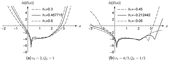
Figure 2. Choose $h_3=h_2=h_1$ and plot the logarithm of the square residual $ln\left[E\left(a\right)\right]$ as a function of a. (a) When $r_0=2$, $Q_0=1$, the curve of the logarithm of the square residuals, (b) corresponds to $r_0=4/3$, $Q_0=1/2$.

Moreover, considering $Q_0$, $r_0$, and corresponding values of $a^{*}$ and $h_1^{*}$, the analytical approximate solutions of charged black holes can be obtained for the different configurations of $Q_0$ and $r_0$. We present an example of $h\left(r\right)$, $f\left(r\right)$, and $A_t\left(r\right)$ for the configuration $Q_0=1$, $r_0=2$, $a^{*}=0.280431$, and $h_1^{*}=0.457715$ after reverting back to the radial coordinate r

$$\begin{array}{ccc}\hfill h\left(r\right)=& & \frac{1}{r^{16}}\{-0.0518821+0.820982r-5.61686r^2+21.6450r^3-51.1353r^4+75.1505r^5\hfill \\ & & -65.8818r^6+30.0274r^7-3.91727r^8-1.57937r^9+0.435328r^{10}-0.00210941r^{11}\hfill \\ & & +0.00976690r^{12}+0.00879167r^{13}+1.10581r^{14}-2.55620r^{15}+r^{16}\hfill \\ & & +0.00329688{(2-r)}^2{r}^{14}ln[1-\frac{2}{r}]\},\hfill \end{array}$$

(37)

$$\begin{array}{ccc}\hfill f\left(r\right)=& & \frac{1}{r^{22}}\{3.76020-65.7119r+518.234r^2-2432.92r^3+7549.78r^4-16254.7r^5\hfill \\ & & +24782.9r^6-26801.9r^7+20235.5r^8-10249.4r^9+3179.84r^{10}-457.973r^{11}\hfill \\ & & +7.15583r^{12}-60.6217r^{13}+81.1245r^{14}-42.4149r^{15}+7.02639r^{16}+1.80243r^{17}\hfill \\ & & 0.634747r^{18}+0.0157998r^{19}+1.11181r^{20}-2.55590r^{21}+r^{22}\},\hfill \end{array}$$

(38)

$$\begin{array}{ccc}\hfill A_t\left(r\right)=& & \frac{1}{r^{11}}\{0.00877198-0.0728020r+0.226609r^2-0.308562r^3+0.144485r^4\hfill \\ & & +0.0102166r^5-0.00262212r^6+0.0244681r^7+0.0581679r^8+0.155568r^9\hfill \\ & & 1.55343r^{10}+1.88217\ast {10}^{-16}{r}^{11}+0.986741r^{11}ln[1-\frac{0.560861}{r}]\}.\hfill \end{array}$$

(39)

The comparison between the analytical approximation solutions obtained by the HAM and numerical solutions is plotted in Figure 3.

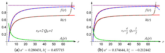
Figure 3. Comparison between analytical approximate solutions and numerical solutions for $h\left(r\right)$, $f\left(r\right)$, and $A_t\left(r\right)$. The solid line represents the analytical approximate solutions, and the dashed line represents the numerical solutions.

It is interesting to check the accuracy of the analytical approximate solutions. We plot these curves describing the deviations (Equations (31) and (32)) of the analytical approximate solutions from the exact solutions, as shown in Figure 4.

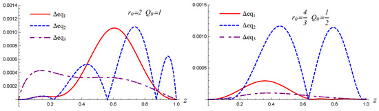
Figure 4. Absolute errors for analytic approximate solutions from two field equations with different values of $r_0$ and $Q_0$. Represented as the deviations of the analytical approximate solutions from the exact solutions. The parameters are the same as used in Figure 3.

In order to compare with the numerical solutions, we will calculate the absolute errors between the analytical approximate and numerical solutions in Figure 5

$$\begin{array}{ccc}\hfill & & \Delta h\left(r\right)=|h^{num}\left(r\right)-h^{ana}\left(r\right)\left]\right|,\Delta f\left(r\right)=|f^{num}\left(r\right)-f^{ana}\left(r\right)\left]\right|,\hfill \\ & & \Delta A_t\left(r\right)=|A_t^{num}\left(r\right)-A_t^{ana}\left(r\right)\left]\right|.\hfill \end{array}$$

(40)

In addition to the relative errors in Figure 6

$$\begin{array}{ccc}\hfill & & \delta h\left(r\right)=\frac{|h^{num}\left(r\right)-h^{ana}\left(r\right)\left]\right|}{h^{num}\left(r\right)}\times 100\%,\delta f\left(r\right)=\frac{|f^{num}\left(r\right)-f^{ana}\left(r\right)\left]\right|}{f^{num}\left(r\right)}\times 100\%,\hfill \\ & & A_t\left(r\right)=\frac{|A_t^{num}\left(r\right)-A_t^{ana}\left(r\right)\left]\right|}{A_t^{num}\left(r\right)}\times 100\%.\hfill \end{array}$$

(41)

We find that the main differences between numerical solutions and analytic approximation solutions occur close to the region far from the black hole.

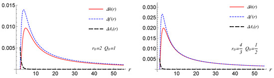
Figure 5. The difference $\Delta h\left(r\right)$ (in red solid) and $\Delta f\left(r\right)$ (in blue dashed) between the analytic approximation solutions and numerical solutions. The parameters are the same as used in Figure 3.

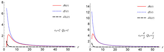
Figure 6. The relative difference $\delta h\left(r\right)$ (in red solid) and $\delta f\left(r\right)$ (in blue dahsed) between the analytic approximation and numerical solutions. The parameters are the same as used in Figure 3.

4. Conclusions and Discussions

In this paper, we discuss the Einstein–Weyl gravity coupled with Maxwell field. Even though the higher derivative curvature terms are introduced into the gravitational action, the field equations always hold no more than second-order derivative for the static and spherical metric functions. Then, we construct numerical solutions for charged black holes with fixed values of charge $Q_0$ and horizon radius $r_0$. Later, we turn to derive the analytical approximation solutions of charged black holes by using the HAM in the Einstein–Maxwell–Weyl gravity. Instead of the convergence-control parameter h obtained from so called “h-curves”, here, we calculate the optimal values of convergence parameter h by evaluating the squared residual error. Moreover, we further compare the analytic approximate solutions with the numerical solutions and check these absolute and relative errors for these solutions, respectively.

In addition, since the approximation is significantly accurate in the entire spacetime outside the event horizon, it can be used for studying the properties of this particular black hole and the various phenomena. The present work is considered as an important work because we confirm that numerical solutions are consistent with an analytical approximate solution for charged black holes.

References

- Stelle, K.S. Renormalization of Higher Derivative Quantum Gravity. Phys. Rev. D 1977, 16, 953. [Google Scholar] [CrossRef]
- Pais, A.; Uhlenbeck, G.E. On Field theories with nonlocalized action. Phys. Rev. 1950, 79, 145–165. [Google Scholar] [CrossRef]
- Holdom, B.; Ren, J. Not quite a black hole. Phys. Rev. D 2017, 95, 084034. [Google Scholar] [CrossRef]
- Lü, H.; Perkins, A.; Pope, C.N.; Stelle, K.S. Black Holes in Higher-Derivative Gravity. Phys. Rev. Lett. 2015, 114, 171601. [Google Scholar] [CrossRef] [PubMed]
- Lü, H.; Perkins, A.; Pope, C.N.; Stelle, K.S. Lichnerowicz Modes and Black Hole Families in Ricci Quadratic Gravity. Phys. Rev. D 2017, 96, 046006. [Google Scholar] [CrossRef]
- Held, A.; Zhang, J. Instability of spherically symmetric black holes in quadratic gravity. Phys. Rev. D 2023, 107, 064060. [Google Scholar] [CrossRef]
- Lin, K.; Pavan, A.B.; Flores-Hidalgo, G.; Abdalla, E. New Electrically Charged Black Hole in Higher Derivative Gravity. Braz. J. Phys. 2017, 47, 419. [Google Scholar] [CrossRef]
- Lin, K.; Qian, W.L.; Pavan, A.B.; Abdalla, E. (Anti-) de Sitter Electrically Charged Black Hole Solutions in Higher-Derivative Gravity. EPL 2016, 114, 60006. [Google Scholar] [CrossRef]
- Zou, D.C.; Wu, C.; Zhang, M.; Yue, R.H. Black holes in the Einstein-Born-Infeld-Weyl gravity. EPL 2019, 128, 40006. [Google Scholar] [CrossRef]
- Wu, C.; Zou, D.C.; Zhang, M. Charged black holes in the Einstein-Maxwell-Weyl gravity. Nucl. Phys. B 2020, 952, 114942. [Google Scholar] [CrossRef]
- Cai, Y.F.; Cheng, G.; Liu, J.; Wang, M.; Zhang, H. Features and stability analysis of non-Schwarzschild black hole in quadratic gravity. JHEP 2016, 1601, 108. [Google Scholar] [CrossRef]
- Zinhailo, A.F. Quasinormal modes of the four-dimensional black hole in Einstein-Weyl gravity. Eur. Phys. J. C 2018, 78, 992. [Google Scholar] [CrossRef]
- Zou, D.C.; Wu, C.; Zhang, M.; Yue, R. Quasinormal modes of charged black holes in Einstein-Maxwell-Weyl gravity. Chin. Phys. C 2020, 44, 055102. [Google Scholar] [CrossRef]
- Sultana, J. Hairy black holes in Einstein-Weyl gravity. Phys. Rev. D 2020, 101, 084027. [Google Scholar] [CrossRef]
- Huang, Y.; Liu, D.J.; Zhang, H. Novel black holes in higher derivative gravity. JHEP 2023, 02, 057. [Google Scholar] [CrossRef]
- Podolsky, J.; Svarc, R.; Pravda, V.; Pravdova, A. Explicit black hole solutions in higher-derivative gravity. Phys. Rev. D 2018, 98, 021502. [Google Scholar] [CrossRef]
- Silveravalle, S.; Zuccotti, A. Phase diagram of Einstein-Weyl gravity. Phys. Rev. D 2023, 107, 6. [Google Scholar] [CrossRef]
- Rezzolla, L.; Zhidenko, A. New parametrization for spherically symmetric black holes in metric theories of gravity. Phys. Rev. D 2014, 90, 084009. [Google Scholar] [CrossRef]
- Kokkotas, K.; Konoplya, R.A.; Zhidenko, A. Non-Schwarzschild black-hole metric in four dimensional higher derivative gravity: Analytical approximation. Phys. Rev. D 2017, 96, 064007. [Google Scholar] [CrossRef]
- Liao, S.J. On the Proposed Homotopy Analysis Techniques for Nonlinear Problems and Its Application. Ph.D. Dissertation, Shanghai Jiao Tong University, Shanghai, China, 1992. [Google Scholar]
- Liao, S.J. Beyond Perturbation: Introduction to the Homotopy Analysis Method, 1st ed.; Chapman and Hall/CRC: Boca Raton, FL, USA, 2003. [Google Scholar]
- Liao, S.J. Homotopy Analysis Method in Nonlinear Differential Equations; Higher Education Press: Beijing, China, 2012. [Google Scholar]
- Zou, D.C.; Meng, B.; Zhang, M.; Li, S.Y.; Lai, M.Y.; Myung, Y.S. Analytical approximate solutions for scalarized AdS black holes. Universe 2023, 9, 26. [Google Scholar] [CrossRef]
- Sultana, J. Obtaining analytical approximations to black hole solutions in higher-derivative gravity using the homotopy analysis method. Eur. Phys. J. Plus 2019, 134, 111. [Google Scholar] [CrossRef]
- Sultana, J. Gravitational Decoupling in Higher Order Theories. Symmetry 2021, 13, 1598. [Google Scholar] [CrossRef]
- Cho, G. Analytic expression of perturbations of Schwarzschild spacetime via Homotopy Analysis Method. arXiv 2020, arXiv:2008.12526. [Google Scholar]
- Liao, S.J. On the homotopy analysis method for nonlinear problems. Appl. Math. Comput. 2004, 147, 499–513. [Google Scholar] [CrossRef]
- Van Gorder, R.A.; Vajravelu, K. On the selection of auxiliary functions, operators, and convergence control parameters in the application of the Homotopy Analysis Method to nonlinear differential equations: A general approach. Commun. Nonlinear Sci. Numer. Simul. 2009, 14, 4078–4089. [Google Scholar] [CrossRef]
- Yin, S.; Chaolu, T. A method to select the initial guess solution, auxiliary linear operator and set of basic functions of homotopy analysis method. In Proceedings of the 2010 International Conference on Intelligent Computing and Integrated Systems, Guilin, China, 22–24 October 2010. [Google Scholar] [CrossRef]
- Xu, H.; Lin, Z.L.; Liao, S.J.; Wu, J.Z.; Majdalani, J. Homotopy based solutions of the Navier–Stokes equations for a porous channel with orthogonally moving walls. Phys. Fluids 2010, 22, 053601. [Google Scholar] [CrossRef]
Disclaimer/Publisher’s Note: The statements, opinions and data contained in all publications are solely those of the individual author(s) and contributor(s) and not of MDPI and/or the editor(s). MDPI and/or the editor(s) disclaim responsibility for any injury to people or property resulting from any ideas, methods, instructions or products referred to in the content. |
© 2023 by the authors. Licensee MDPI, Basel, Switzerland. This article is an open access article distributed under the terms and conditions of the Creative Commons Attribution (CC BY) license (https://creativecommons.org/licenses/by/4.0/).