Phase Space Analysis of Barrow Agegraphic Dark Energy

Abstract

Using the Barrow entropy and considering the timescale as IR cutoff, a new holographic dark energy model named Barrow agegraphic dark energy (BADE) was proposed. We use phase space analysis method to discuss the evolution of the universe in three different mode of BADE ($Q=0$; $Q=3\alpha H({\rho }_m+{\rho }_D)$; $Q=H(\alpha {\rho }_m+\beta {\rho }_D)$). We find the attractor which represents the dark energy-dominated era exists in all cases. In the case $Q=0$ and $Q=H(\alpha {\rho }_m+\beta {\rho }_D)$ with $\beta =0$, the attractor can behave as the cosmological constant, and these models can used to mimic the cosmological constant.

1. Introduction

The cosmological observations [1,2,3,4,5,6] indicate that the present universe undergoes an accelerating expansion. The dark energy theory is an extremely good representation of cosmology for a host of situations of practical and astronomical interest. The simplest candidate of dark energy is the cosmological constant $\mathsf{\Lambda }$ and the corresponding model is called the $\mathsf{\Lambda }$CDM model. It gives a detailed account of the evolution of the universe, and of the nearly scale-invariant primordial power spectra that fit the results of cosmological observations [7]. However, it is still confronted with some obstacles such as cosmic coincidence and fine-tuning issues [8,9]. Thus, in order to explain the present accelerating expansion of the universe, lots of cosmological models had been introduced, for example, holographic dark energy [10,11,12,13].

There are, of course, many compelling reasons to begin a study of dark energy with a review of the infrared (IR) cutoff. As a candidate of dark energy, holographic dark energy (HDE) arised from the holographic principle with an IR cutoff of Hubble horizon scale [10,11,12] and attracted lots of researcher’s attention [14,15,16,17,18,19,20,21,22,23,24,25,26,27,28,29,30], and it also coincident with the observational data [31,32,33,34]. Because it failed to describe the evolutionary history of the universe [12,13], the physicists get motivated to study different IR cutoffs in HDE model. Since the HDE models are based on the IR cutoff and the horizon entropy, different IR cutoff and horizon entropy will lead to different HDE model. When the age of the universe was considered as the IR cutoff, the agegraphic dark energy model (ADE) was introduced [35]. Although the causality problem can be avoided in this model and the accelerated expansion is also realized, this model fails to describe a matter-dominated epoch in the very early evolution era and mimic cosmological constants in late time. To solve this problem, a new agegraphic dark energy model (NADE) was proposed by choosing the time scale as the conformal time [36], in which the coincidence problem could be solved naturally [37]. In addition, when a non-minimal coupling between the q-field and matter was introduced, the dark energy density parameter of ADE can be adjusted to the present values [38]. However, since the squared speeds of sound are negative, both ADE and NADE are classically unstable [39]. When the Tsallis entropy was introduced into ADE, Tsallis agegraphic dark energy model (TADE) [40] and a new Tsallis agegraphic dark energy model (NTADE) [41] were proposed. By analyzing the evolution of the squared speeds of sound, it was found that TADE is stable at the classical level when there exists a mutual interaction between dark matter and dark energy [40], while NTADE can be stable only in the future [41]. The behaviour of the squared speeds of sound was also discussed in Kaniadakis agegraphic dark energy model [42] and quantum loop-correction dark energy model [43], the first model is stable only in the future, while the second one can be stable classically for the interaction case.

Recently, Barrow showed that quantum gravitational effects may introduce intricate, fractal features on the black hole structures [44]. This complex structure leads to finite volume and infinite (or finite) area. Based on this modification, the entropy of the black holes no longer obeys the area law and is modified as $S_B={(A/A_0)}^{1+\mathsf{\Delta }/2}$ which is named as the Barrow entropy. The parameter A and $A_0$ denote the standard horizon area and the Planck area, respectively. $\mathsf{\Delta }$ is the deformation parameter, which represents the amount of the quantum gravitational deformation effects on the horizon structure. The Bekenstein–Kawking entropy can be recovered for $\mathsf{\Delta }=0$, and $\mathsf{\Delta }=1$ denotes the most intricate fractal structure. When the Barrow entropy was introduced into HDE, a new HDE named Barrow holographic dark energy (BHDE) [45,46] was proposed. Then, by choosing the age of the universe and the conformal time as the IR cutoff, Barrow agegraphic dark energy (BADE) was proposed in Ref. [47], in which the evolutions of the cosmological parameters and the stability of these models were analyzed, and it was found that BADE with the conformal time as IR cutoff can be stable in the past.

In order to analyze the evolution of the universe, we use the powerful tool called phase space analysis method in BADE models, which was extensively used in the late-time stable solution and the evolution of the universe. The field of application include f(R) gravity [48], loop quantum gravity [49,50], and another modified gravitational theories [51,52,53,54,55,56,57,58,59,60,61,62,63,64,65,66,67,68]. In ADE, by considering an interaction term between dark matter and dark energy, the results of the phase space analysis show that the transient acceleration exists in this model, but it can not describe the evolutionary history of the universe [69]. When the ADE was introduced into Brans-Dicke cosmology, it also failed to describe the evolutionary history of the universe [70]. After the phase space analysis method was applied to TADE, it was found that TADE can describe the evolutionary history of the universe and mimic the cosmological constant after introducing an interaction term between dark matter and dark energy [68]. In this paper, we will apply the phase space analysis method to discuss whether the evolutionary history of the universe can be described by BADE.

This paper is organized as follows. In Section 2, we briefly review BADE model. In Section 3, we study the phase space behavior of BADE models. In Section 4, we discuss the evolution of the Hubble parameter for BADE models. Our main conclusions are presented in Section 5.

2. Background

The energy density of the Barrow holographic dark energy model is given by [45,46]

$${\rho }_d=B{L}^{\mathsf{\Delta }-2},$$

(1)

where B is a parameter with dimensions ${\left[L\right]}^{-2-\mathsf{\Delta }}$ and L is the IR cutoff. Considering the conformal time of the universe as the IR cutoff, one gets [47]

$${\rho }_d=B{\eta }^{\mathsf{\Delta }-2},$$

(2)

with

$$\eta ={\int }_0^a\frac{da}{H{a}^2},$$

(3)

where a is the scale factor with $\eta$ being conformal time and $dt=ad\eta$, and H is the Hubble parameter.

The metric of a homogeneous and isotropic flat FLRW universe takes the form

$$\begin{array}{c}\hfill d{s}^2=-d{t}^2+a^2\left(t\right)\left[d{r}^2+r^2(d{\theta }^2+si{n}^2\theta d{\varphi }^2)\right],\end{array}$$

(4)

and the Friedmann Equation is given as

$$\begin{array}{c}\hfill H^2=\frac{1}{3m_p^2}({\rho }_r+{\rho }_m+{\rho }_D),\end{array}$$

(5)

where $m_p^2=\frac{1}{8\pi G}$, ${\rho }_m$, ${\rho }_r$ and ${\rho }_D$ corresponding to the energy density of three different matter: pressureless matter, radiation and BADE. Then, the conservation equations are

$$\dot{{\rho }_r}+4H{\rho }_r=0,$$

(6)

$$\dot{{\rho }_m}+3H{\rho }_m=Q,$$

(7)

$$\dot{{\rho }_D}+3H(1+{\omega }_D){\rho }_D=-Q.$$

(8)

Here, ${\omega }_D=\frac{p_D}{{\rho }_D}$ is the equation of the state parameter of BADE, Q denotes an interaction between the pressureless matter and BADE. For $Q>0$, energy transfer from BADE to pressureless matter, and energy transfer from pressureless matter to BADE for $Q<0$.

By introducing dimensionless parameters of density

$$x={\mathsf{\Omega }}_m=\frac{{\rho }_m}{3m_p^2{H}^2},y={\mathsf{\Omega }}_y=\frac{{\rho }_D}{3m_p^2{H}^2},r={\mathsf{\Omega }}_r=\frac{{\rho }_r}{3m_p^2{H}^2},\sigma =\frac{Q}{3m_p^2{H}^3},z=\frac{1}{aH\eta },$$

(9)

the Friedmann Equation (5) can be written as

$$x+y+r=1.$$

(10)

Taking the time derivative of the energy density of BADE (2), we obtain the equation of state of BADE

$${\omega }_D=-1-\frac{\sigma }{3y}-\frac{\mathsf{\Delta }-2}{3}z.$$

(11)

Here, the conservation Equation (8) and the relation $\dot{\eta }=1/a$ is used.

Combining Equations (5)–(8) and (11), we get

$$\frac{\dot{H}}{H^2}=-2+2y+\frac{x}{2}+\frac{\sigma }{2}+\frac{\mathsf{\Delta }-2}{2}yz.$$

(12)

Furthermore, the deceleration parameter can be expressed as

$$q=-1-\frac{\dot{H}}{H^2}.$$

(13)

Defining’ $=d/d\left(lna\right)$ and using Equations (7)–(9) and (12), we obtain the autonomous dynamical system of BADE model

$$\begin{array}{c}{x}^{\prime }=-3x+\sigma +2x\left(2-2y-\frac{x}{2}-\frac{\sigma }{2}-\frac{\mathsf{\Delta }-2}{2}yz\right),\hfill \\ y^{\prime }=(\mathsf{\Delta }-2)yz+2y\left(2-2y-\frac{x}{2}-\frac{\sigma }{2}-\frac{\mathsf{\Delta }-2}{2}yz\right),\hfill \\ z^{\prime }=-z-z^2+z\left(2-2y-\frac{x}{2}-\frac{\sigma }{2}-\frac{\mathsf{\Delta }-2}{2}yz\right),\hfill \end{array}$$

(14)

3. Phase Space Analysis

In order to discuss the evolution of the universe in BADE model, we apply the phase space analysis method to this model.

In the dynamical system, we can get the critical points by solving

$$x^{\prime }=y^{\prime }=z^{\prime }=0.$$

(15)

After the critical points are obtained, the stability of these points will be analyzed. According to the linear stability theory, the stability of critical points is determined by the eigenvalues of the Jacobian matrix for the autonomous dynamical system. The critical points can be divided into three types: (i) attractor with all eigenvalues negative, the state is stable; (ii) repeller with all eigenvalues positive, corresponding to an unstable state; (iii) saddle point with at least two eigenvalues signs are opposite.

3.1. Non-Interacting $Q=0$

For the case $Q=0$, we get $\sigma =0$. By solving the equations $x^{\prime }=y^{\prime }=z^{\prime }=0$, we list six different points in Table 1.

Table 1. Critical points and the stability in BADE model with $Q=0$.

$\mathit{Labels}$	$\mathit{Critical}\mathit{Points}(\mathit{x},\mathit{y},\mathit{z})$	${\mathit{\omega }}_{\mathit{D}}$	q	$\mathit{Eigenvalues}$	$\mathit{Conditions}$	$\mathit{Points}$
$A_1$	$(0,0,0)$	$-1$	1	$(4,1,1)$	$0<\mathsf{\Delta }<1$	$Unstable$
$A_2$	$(0,0,1)$	$-1-\frac{\mathsf{\Delta }-2}{3}$	1	$(-1,1,2+\mathsf{\Delta })$	$0<\mathsf{\Delta }<1$	$Saddle$
$A_3$	$(1,0,0)$	$-1$	$\frac{1}{2}$	$(3,-1,\frac{1}{2})$	$0<\mathsf{\Delta }<1$	$Saddle$
$A_4$	$(1,0,\frac{1}{2})$	$-1+\frac{2-\mathsf{\Delta }}{6}$	$\frac{1}{2}$	$(-1,-\frac{1}{2},\frac{4+\mathsf{\Delta }}{2})$	$0<\mathsf{\Delta }<1$	$Saddle$
$A_5$	$(0,1,0)$	$-1$	$-1$	$(-4,-3,-1)$	$0<\mathsf{\Delta }<1$	$Stable$
$A_6$	$(0,1,-\frac{2}{\mathsf{\Delta }})$	$-1+\frac{2(\mathsf{\Delta }-2)}{3\mathsf{\Delta }}$	$-\frac{2}{\mathsf{\Delta }}$	$(1,-\frac{2(2+\mathsf{\Delta })}{\mathsf{\Delta }},-\frac{4+\mathsf{\Delta }}{\mathsf{\Delta }})$	$0<\mathsf{\Delta }<1$	$Saddle$

Points $A_1$ and $A_2$: Corresponding to decelerated phase in the radiation-dominated era, since $x=y=0$ and $q=1$, the equation of state ${\omega }_D$ for $A_1$ and $A_2$ are $-1$ and $-1-\frac{2-\mathsf{\Delta }}{3}$, respectively.

Points $A_3$ and $A_4$: Since $x=1$, $y=0$ and $q=\frac{1}{2}$, they corresponds to decelerated phase in the matter-dominated epoch, and the equations of state ${\omega }_D$ are negative.

Point $A_5$ and $A_6$: Since $x=0$ and $y=1$, these points represent the dark energy-dominated epoch with an accelerated phase. For point $A_5$, since ${\omega }_D=-1$ and $q=-1$, it can mimic the cosmological constant $\mathsf{\Lambda }$.

Using the linear stability theory and after some tedious calculations. We give the corresponding eigenvalues and stability conditions in Table 1. From this table, we can see that the radiation-dominated point $A_1$ is unstable, the dark energy-dominated point $A_5$ is stable, and the rest points are saddle points. According to this result, the universe stems from the radiation-dominated era $A_1$, followed by the matter-dominated era $A_3$, and eventually evolves into an accelerated expansion epoch $A_5$. This evolutionary case is shown in Figure 1 in which we have plotted the evolutionary trajectories of these points. From this figure, we can see that point $A_5$ behaves as an attractor, and the universe will eventually evolve into an epoch depicted by the cosmological constant.

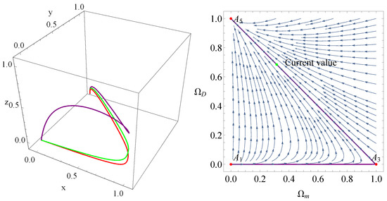
Figure 1. Phase space trajectories for BADE with $Q=0$. The left panel is plotted for $B=50$, $\mathsf{\Delta }=0.1,0.2,0.3$. The right panel shows the phase diagram $({\mathsf{\Omega }}_m,{\mathsf{\Omega }}_D)$, the purple line in the right panel is plotted for $B=50$, $\mathsf{\Delta }=0.3$.

3.2. Interacting $Q=3\alpha H({\rho }_m+{\rho }_D)$

In this subsection, we consider the case $Q=3\alpha H({\rho }_m+{\rho }_D)$ [47], which indicates $\sigma =3\alpha ({\mathsf{\Omega }}_m+{\mathsf{\Omega }}_D)=3\alpha (x+y)$. Here, $\alpha$ is a positive parameter and we choose $0<\alpha <1$. Then, solving the equations $x^{\prime }=y^{\prime }=z^{\prime }=0$ and using the linear stability theory, we obtain six critical points and the corresponding stability conditions, which are shown in Table 2 and Table 3. The expression of $E_{1,2}$ in Table 3 are

$$E_{1,2}=\frac{\mathsf{\Delta }(4+\mathsf{\Delta })[(9\alpha -2)\mathsf{\Delta }-8]\pm \sqrt{\chi }}{{\mathsf{\Delta }}^2{(4+\mathsf{\Delta })}^2},$$

(16)

with

$$\chi =-{\mathsf{\Delta }}^2{(4+\mathsf{\Delta })}^2\{[3\alpha (\mathsf{\Delta }+4)({\mathsf{\Delta }}^2+4\mathsf{\Delta }+12)-(\mathsf{\Delta }+6)({\mathsf{\Delta }}^2+6\mathsf{\Delta }+16)-81{\alpha }^2\mathsf{\Delta }]\mathsf{\Delta }-64\}.$$

(17)

Table 2. Critical points of the autonomous system in BADE model with the interaction $Q=3\alpha H({\rho }_m+{\rho }_D)$.

$\mathit{Labels}$	$\mathit{Critical}\mathit{Points}(\mathit{x},\mathit{y},\mathit{z})$	${\mathit{\omega }}_{\mathit{D}}$	q
$B_1$	$(0,0,0)$	$-1-2\alpha$	1
$B_2$	$(0,0,1)$	$-1-2\alpha -\frac{\mathsf{\Delta }-2}{3}$	1
$B_3$	$(1,0,0)$	−	$\frac{1}{2}(1-3\alpha )$
$B_4$	$(1,0,\frac{1}{2}(1-3\alpha ))$	−	$\frac{1}{2}(1-3\alpha )$
$B_5$	$(\alpha ,1-\alpha ,0)$	$-1-\frac{\alpha }{1-\alpha }$	$-1$
$B_6$	$(\frac{3\alpha \mathsf{\Delta }}{4+\alpha },\frac{4+\mathsf{\Delta }-3\alpha \mathsf{\Delta }}{4+\mathsf{\Delta }},-\frac{2}{\mathsf{\Delta }})$	$\frac{{(4+\mathsf{\Delta })}^2}{3\mathsf{\Delta }\left[\right(3\alpha -1)\mathsf{\Delta }-4]}$	$-\frac{2}{\mathsf{\Delta }}$

Table 3. Eigenvalues and the stability of critical points in BADE model with the interaction $Q=3\alpha H({\rho }_m+{\rho }_D)$.

$\mathit{Labels}$	$\mathit{Eigenvalues}$	$\mathit{Conditions}$	$\mathit{Points}$
$B_1$	$(4,1,1+3\alpha )$	$0<\mathsf{\Delta }<1,0<\alpha <1$	$Unstable$
$B_2$	$(-1,1+3\alpha ,2+\mathsf{\Delta })$	$0<\mathsf{\Delta }<1,0<\alpha <1$	$Saddle$
$B_3$	$(\frac{1}{2}(1-3\alpha ),3(1-\alpha ),-1-3\alpha )$	$0<\mathsf{\Delta }<1,0<\alpha <1$	$Saddle$
$B_4$	$(\frac{1}{2}(3\alpha -1),-1-3\alpha ,\frac{1}{2}(4+\mathsf{\Delta }-3\alpha \mathsf{\Delta }))$	$0<\mathsf{\Delta }<1,0<\alpha <\frac{1}{3}or\frac{1}{3}<\alpha <1$	$Saddle$
$B_5$	$(-4,-1,-3(1-\alpha \left)\right)$	$0<\mathsf{\Delta }<1,0<\alpha <1$	$Stable$
$B_6$	$-\frac{2(2+\mathsf{\Delta })}{\mathsf{\Delta }},E_1,E_2$	$0<\mathsf{\Delta }<1,0<\alpha <1$	$Saddle$

From Table 2 and Table 3, we can find these results:

Points $B_1$ and $B_2$: They represent decelerated phase in the radiation-dominated era, the equation of state ${\omega }_D$ is determined by the value of $\alpha$ and $\mathsf{\Delta }$. Point $B_1$ is unstable while $B_2$ is a saddle point.

Points $B_3$ and $B_4$: These points represent the matter-dominated epoch. For $0<\alpha <\frac{1}{3}$, they denote a decelerated phase, while they are an accelerated one for $\frac{1}{3}<\alpha <1$. Furthermore, both of them are saddle points.

Point $B_5$ and $B_6$: These points are determined by $\alpha$ and $\mathsf{\Delta }$. For the small value of $\alpha$, they represent the dark energy-dominated era with an accelerated phase.

According to these results, we can see that the universe evolves from the radiation-dominated era $B_1$ into the matter-dominated era $B_3$, and eventually enters an accelerated expansion epoch $B_5$. Although point $B_5$ is an attractor, it can not mimic the cosmological constant. The evolutionary curves are depicted in Figure 2.

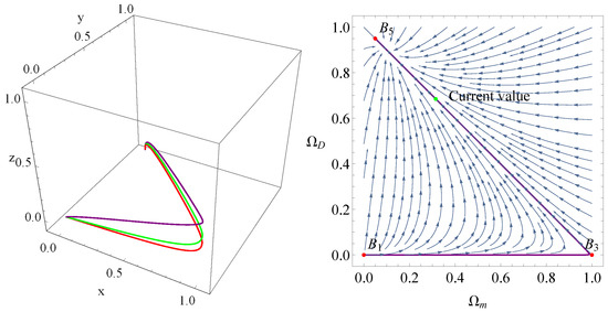
Figure 2. Phase space trajectories for BADE with $Q=3\alpha H({\rho }_m+{\rho }_D)$. In the left part, $B=80$, $\alpha =0.05$, $\mathsf{\Delta }=0.1,0.2,0.3$. The right panel shows the phase diagram $({\mathsf{\Omega }}_m,{\mathsf{\Omega }}_D)$, the purple line in the right panel is plotted for $B=80$, $\alpha =0.05$, $\mathsf{\Delta }=0.1$.

3.3. Interacting $Q=H(\alpha {\rho }_m+\beta {\rho }_D)$

In the case $Q=H(\alpha {\rho }_m+\beta {\rho }_D)$ [71,72], we get $\sigma =\alpha {\mathsf{\Omega }}_m+\beta {\mathsf{\Omega }}_D=\alpha x+\beta y$ in which $\alpha$ and $\beta$ are the interacting parameters and we consider $0<\alpha <1$ and $0<\beta <1$. After solving the equations $x^{\prime }=y^{\prime }=z^{\prime }=0$ and considering the linear stability theory, we obtain six critical points which are shown in Table 4, and the corresponding stability conditions for these points are shown in Table 5.

Table 4. Critical points of the autonomous system in BADE model with the interaction term $Q=H(\alpha {\rho }_m+\beta {\rho }_D)$.

$\mathit{Labels}$	$\mathit{Critical}\mathit{Points}(\mathit{x},\mathit{y},\mathit{z})$	${\mathit{\omega }}_{\mathit{D}}$	q
$C_1$	$(0,0,0)$	$-1-\frac{\alpha +\beta }{3}$	1
$C_2$	$(0,0,1)$	$-1-\frac{\alpha +\beta }{3}-\frac{\mathsf{\Delta }-2}{3}$	1
$C_3$	$(1,0,0)$	−	$\frac{1}{2}(1-\alpha )$
$C_4$	$(1,0,\frac{1}{2}(1-\alpha ))$	−	$\frac{1}{2}(1-\alpha )$
$C_5$	$(\frac{\beta }{3-\alpha +\beta },\frac{3-\alpha }{3-\alpha +\beta },0)$	$-1+\frac{\beta }{\alpha -3}$	$-1$
$C_6$	$(\frac{\beta \mathsf{\Delta }}{4+\mathsf{\Delta }(1-\alpha +\beta )},\frac{4+\mathsf{\Delta }(1-\alpha )}{4+\mathsf{\Delta }(1-\alpha +\beta )},-\frac{2}{\mathsf{\Delta }})$	$-\frac{(\mathsf{\Delta }+4)\left[\right(\alpha -\beta -1)\mathsf{\Delta }-4]}{3\mathsf{\Delta }\left[\right(\alpha -1)\mathsf{\Delta }-4]}$	$-\frac{2}{\mathsf{\Delta }}$

Table 5. Eigenvalues and the stability of critical points in BADE model with the interaction term $Q=H(\alpha {\rho }_m+\beta {\rho }_D)$.

$\mathit{Labels}$	$\mathit{Eigenvalues}$	$\mathit{Conditions}$	$\mathit{Points}$
$C_1$	$(4,1,1+\alpha )$	$0<\mathsf{\Delta }<1,0<\alpha <1,0<\beta <1$	$Unstable$
$C_2$	$(-1,1+\alpha ,2+\mathsf{\Delta })$	$0<\mathsf{\Delta }<1,0<\alpha <1,0<\beta <1$	$Saddle$
$C_3$	$(\frac{1}{2}(1-\alpha ),3-\alpha ,-1-\alpha )$	$0<\mathsf{\Delta }<1,0<\alpha <1,0<\beta <1$	$Saddle$
$C_4$	$(\frac{1}{2}(\alpha -1),-1-\alpha ,\frac{1}{2}[4+\mathsf{\Delta }(1-\alpha )])$	$0<\mathsf{\Delta }<1,0<\alpha <1,0<\beta <1$	$Saddle$
$C_5$	$(-4,-1,-3+\alpha )$	$0<\mathsf{\Delta }<1,0<\alpha <1,0<\beta <1$	$Stable$
$C_6$	$-\frac{2(2+\mathsf{\Delta })}{\mathsf{\Delta }},F_1,F_2$	$0<\mathsf{\Delta }<1,0<\alpha <1,0<\beta <1$	$Saddle$

The expression of $F_{1,2}$ in Table 5 are

$$F_{1,2}=\frac{16+[4-8\alpha +2\beta +(\alpha -1)(\alpha -\beta )\mathsf{\Delta }]\mathsf{\Delta }\pm \sqrt{\xi }}{2\mathsf{\Delta }\left[\right(\alpha -\beta -1)\mathsf{\Delta }-4]}$$

(18)

with

$$\begin{array}{cc}\xi \hfill & =(\alpha -1)[{(\alpha -2)}^2(\alpha -1)-2(\alpha -4)(\alpha -1)\beta +(\alpha -5){\beta }^2]{\mathsf{\Delta }}^4\hfill \\ \hfill & -4[2(\alpha -2)(\alpha -1)(2\alpha -3)-(\alpha -1)(5\alpha -18)\beta +(\alpha -5){\beta }^2]{\mathsf{\Delta }}^3\hfill \\ \hfill & +4[52+24{\alpha }^2+(44+\beta )\beta -8\alpha (9+2\beta )]{\mathsf{\Delta }}^2+64(6-4\alpha +\beta )\mathsf{\Delta }+256.\hfill \end{array}$$

(19)

Table 4 and Table 5 show these results:

Points $C_1$ and $C_2$: Since $x=y=0$ and $q=1$, they correspond to decelerated phase in the radiation-dominated era. The equation of state ${\omega }_D$ of these points are fully determined by the value of $\alpha$, $\beta$ and $\mathsf{\Delta }$. Point $C_1$ is an unstable point while $C_2$ is a saddle one.

Points $C_3$ and $C_4$: These points represent the matter-dominated epoch with a decelerated phase. Furthermore, both of them are saddle points.

Points $C_5$ and $C_6$: For these points, they are determined by the value of $\alpha$, $\beta$ and $\mathsf{\Delta }$. For the small value of $\alpha$ and $\beta$, both of these points indicate the dark energy-dominated epoch with an accelerated phase. For point $C_5$ with $\beta =0$, we obtain $x=0$, $y=1$, and $q=-1$, which denotes the evolutionary epoch depicted by the cosmological constant. Thus, for $\beta =0$, point $C_5$ can mimic the cosmological constant, and the universe will eventually evolve into the epoch depicted by the cosmological constant since point $C_5$ is an attractor.

In Figure 3 and Figure 4, we have plotted the evolutionary curves of the universe in BADE model with the interaction term $Q=H(\alpha {\rho }_m+\beta {\rho }_D)$. In Figure 4, the value of parameter $\beta$ is zero. We can see that the universe stems from the point $C_1$, enters into $C_3$, and eventually evolves into $C_5$ which represents the epoch depicted by the cosmological constant.

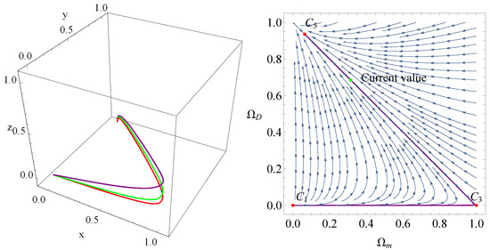
Figure 3. Phase space trajectories for BADE with $Q=H(\alpha {\rho }_m+\beta {\rho }_D)$. The left panel is plotted for $B=80$, $\alpha =0.1$, $\beta =0.2$, $\mathsf{\Delta }=0.1,0.2,0.3$. The right panel shows the phase diagram $({\mathsf{\Omega }}_m,{\mathsf{\Omega }}_D)$, the purple line in the right panel is plotted for $B=80$, $\alpha =0.1$, $\beta =0.2$, $\mathsf{\Delta }=0.3$.

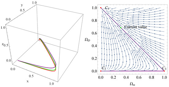
Figure 4. Phase space trajectories for BADE with $Q=H(\alpha {\rho }_m+\beta {\rho }_D)$. The left panel is plotted for $B=80$, $\alpha =0.1$, $\beta =0$, $\mathsf{\Delta }=0.1,0.2,0.3$. The right panel shows the phase diagram $({\mathsf{\Omega }}_m,{\mathsf{\Omega }}_D)$, the purple line in the right panel is plotted for $B=80$, $\alpha =0.1$, $\beta =0$, $\mathsf{\Delta }=0.3$.

4. Hubble Diagram

In order to discuss the difference of cosmological evolution between BADE and $\mathsf{\Lambda }$CDM, we have plotted the evolutionary curves of Hubble parameter for these models in Figure 5, Figure 6 and Figure 7. The error bars in these figures denote the observational Hubble parameter data [73,74]. In Figure 5, we have plotted the evolutionary curves of the Hubble parameter for the non-interacting case $Q=0$. The left panel shows the evolutionary curves of the Hubble parameter in BADE, and the curves approach the one in $\mathsf{\Lambda }$CDM with a small $\mathsf{\Delta }$. In the right panel, for a large value of B, these curves in BADE overlap with the one in $\mathsf{\Lambda }$CDM. For the interacting case $Q=3\alpha H({\rho }_m+{\rho }_D)$, the evolutionary curves deviate from the one in $\mathsf{\Lambda }$CDM in the future which is shown in both the left and right panel of Figure 6. The evolutionary curves of Hubble parameter for the interacting case $Q=H(\alpha {\rho }_m+\beta {\rho }_D)$ are plotted in Figure 7. The left panel of Figure 7 shows that the value of $\alpha$ has a slight influence on the evolutionary curves of the Hubble parameter. The right panel of Figure 7 shows the same results as the right panel of Figure 5. Thus, for the non-interacting case $Q=0$ and the interacting case $Q=H(\alpha {\rho }_m+\beta {\rho }_D)$ with $\beta =0$, BADE can mimic the cosmological constant in the late-time evolution epoch.

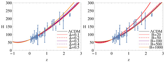
Figure 5. Evolutionary curves of H for non-interacting $Q=0$. The left panel is plotted for $B=50$, while the right one is for $\mathsf{\Delta }=0.3$.

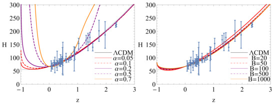
Figure 6. Evolutionary curves of H for interacting $Q=3\alpha H({\rho }_m+{\rho }_D)$. The left panel is plotted for $B=80,\mathsf{\Delta }=0.1$, while the right one is for $\alpha =0.05,\mathsf{\Delta }=0.1$.

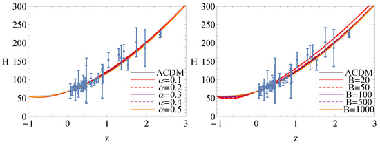
Figure 7. Evolutionary curves of H for interacting $Q=H(\alpha {\rho }_m+\beta {\rho }_D)$. The left panel is plotted for $B=80,\beta =0,\mathsf{\Delta }=0.1$, while the right one is for $\alpha =0.1,\beta =0,\mathsf{\Delta }=0.1$.

5. Conclusions

Using the Barrow entropy and considering the timescale as IR cutoff, a new holographic dark energy model named Barrow agegraphic dark energy was proposed. In this paper, by choosing the conformal time as the IR cutoff, we study the evolution of the universe in BADE model. In this model, we analyze three different cases: (i) $Q=0$; (ii) $Q=3\alpha H({\rho }_m+{\rho }_D)$; (iii) $Q=H(\alpha {\rho }_m+\beta {\rho }_D)$. Through the method of phase space and stability analysis, we conclude that the attractor which represents the dark energy-dominated era exists in all cases and both of them can describe the expansion history of the universe. For the case $Q=0$, there exists six critical points, point $A_1$ is unstable and denotes the radiation-dominated era, and point $A_5$ is stable and represents the dark energy-dominated era. Since ${\omega }_D=-1$ and $q=-1$, point $A_5$ can mimic the cosmological constant. The behaviour of phase space shows that the universe can stem from the radiation-dominated era $A_1$, pass through the matter-dominated era $A_3$, and then enter into the dark energy-dominated era $A_5$. So, the evolutionary history of the universe can be described by this model. For the case $Q=3\alpha H({\rho }_m+{\rho }_D)$, there also exists six critical points. Although point $B_5$ is stable and can represent the dark energy-dominated era for the small value of $\alpha$, it can not mimic the cosmological constant since $\alpha \ne 0$. For the case $Q=H(\alpha {\rho }_m+\beta {\rho }_D)$, there is six critical points. Point $C_5$ is a stable point, and it can mimic the cosmological constant. The evolutionary history of the universe can be described by this case with $\beta =0$.

Since BADE can mimic the cosmological constant, we depict the evolutionary curves of the Hubble parameter to compare BADE with $\mathsf{\Lambda }$CDM. The results show that the evolutionary curves of Hubble parameter in BADE overlap with $\mathsf{\Lambda }$CDM at the late-time evolution epoch in the cases $Q=0$ and $Q=H(\alpha {\rho }_m+\beta {\rho }_D)$ with $\beta =0$.

References

- Perlmutter, S.; Aldering, G.; Goldhaber, G.; Knop, R.; Nugent, P.; Castro, P.; Deustua, S.; Fabbro, S.; Goobar, A.; Groom, D.; et al. Measurements of Ω and Λ from 42 High-Redshift supernovae. Astrophys. J. 1999, 517, 565. [Google Scholar] [CrossRef]
- Riess, A.G.; Filippenko, A.V.; Challis, P.; Clocchiatti, A.; Diercks, A.; Garnavich, P.M.; Gilliland, R.L.; Hogan, G.J.; Jha, S.; Kirshner, R.P.; et al. Observational evidence from supernovae for an accelerating universe and a cosmological constant. Astrophys. J. 1998, 116, 1009. [Google Scholar] [CrossRef]
- Spergel, D.N.; Verde, L.; Peiris, H.V.; Komatsu, E.; Nolta, M.R.; Bennett, C.L.; Halpern, M.; Hinshaw, G.; Jarosik, N.; Kogut, A.; et al. First-Year Wilkinson Microwave Anisotropy Probe (WMAP) observations: Determination of cosmological parameters. Astrophys. J. Suppl. 2003, 148, 175. [Google Scholar] [CrossRef]
- Spergel, D.N.; Bean, R.; Doré, O.; Nolta, M.R.; Bennett, C.L.; Dunkley, J.; Hinshaw, G.; Jarosik, N.E.; Komatsu, E.; Page, L.; et al. Three-Year Wilkinson Microwave Anisotropy Probe (WMAP) observations: Implications for cosmology. Astrophys. J. Suppl. 2007, 170, 337. [Google Scholar] [CrossRef]
- Tegmark, M.; Strauss, M.A.; Blanton, M.R.; Abazajian, K.; Dodelson, S.; Sandvik, H.; Wang, X.; Weinberg, D.H.; Zehavi, I.; Bahcall, N.A.; et al. Cosmological parameters from SDSS and WMAP. Phys. Rev. D 2004, 69, 103501. [Google Scholar] [CrossRef]
- Eisenstein, D.J.; Zehavi, I.; Hogg, D.W.; Scoccimarro, R.; Blanton, M.R.; Nichol, R.C.; Scranton, R.; Seo, H.J.; Tegmark, M.; Zheng, Z.; et al. Detection of the baryon acoustic pPeak in the large-scale correlation function of SDSS luminous red galaxies. Astrophys. J. 2005, 633, 560. [Google Scholar] [CrossRef]
- Planck Collaboration; Ade, P.A.R.; Aghanim, N.; Arnaud, M.; Ashdown, M.; Aumont, J.; Baccigalupi, C.; Banday, A.J.; Barreiro, R.B.; Bartlett, J.G.; et al. Planck 2015 results XIII. cosmological parameters. Astron. Astrophys. 2016, 594, A13. [Google Scholar] [CrossRef]
- Weinberg, S. The cosmological constant problem. Rev. Mod. Phys. 1989, 61, 1. [Google Scholar] [CrossRef]
- Steinhardt, P.; Wang, L.; Zlatev, I. Cosmological tracking solutions. Phys. Rev. D 1999, 59, 123504. [Google Scholar] [CrossRef]
- Cohen, A.G.; Kaplan, D.B.; Nelson, A.E. Effective field theory, black holes, and the cosmological constant. Phys. Rev. Lett. 1999, 82, 4971. [Google Scholar] [CrossRef]
- Hsu, S. Entropy bounds and dark energy. Phys. Lett. B 2004, 594, 13–16. [Google Scholar] [CrossRef]
- Li, M. A model of holographic dark energy. Phys. Lett. B 2004, 603, 1–5. [Google Scholar] [CrossRef]
- Wang, S.; Wang, Y.; Li, M. Holographic dark energy. Phys. Rep. 2017, 696, 1–57. [Google Scholar] [CrossRef]
- Horava, P.; Minic, D. Probable values of the cosmological constant in a holographic theory. Phys. Rev. Lett. 2000, 85, 1610. [Google Scholar] [CrossRef]
- Shen, J.; Wang, B.; Abdalla, E.; Su, R.K. Constraints on the dark energy from the holographic connection to the small l CMB suppression. Phys. Lett. B 2005, 609, 200–205. [Google Scholar] [CrossRef]
- Guberina, B.; Horvat, R.; Nikolic, H. Non-saturated holographic dark energy. J. Cosmol. Astropart. Phys. 2007, 2007, 012. [Google Scholar] [CrossRef]
- Sheykhi, A. Interacting agegraphic dark energy models in non-flat universe. Phys. Lett. B 2009, 680, 113. [Google Scholar] [CrossRef]
- Sheykhi, A. Interacting holographic dark energy in Brans–Dicke theory. Phys. Lett. B 2009, 681, 205. [Google Scholar] [CrossRef]
- Sheykhi, A. Interacting agegraphic tachyon model of dark energy. Phys. Lett. B 2010, 682, 329. [Google Scholar] [CrossRef]
- Sheykhi, A.; Karami, K.; Jamil, M.; Kazemi, E.; Haddad, M. Holographic dark energy in Brans–Dicke theory with logarithmic correction. Gen. Relativ. Gravit. 2012, 44, 623–638. [Google Scholar] [CrossRef]
- Ghaffari, S.; Dehghani, M.; Sheykhi, A. Holographic dark energy in the DGP braneworld with Granda-Oliveros cutoff. Phys. Rev. D 2014, 89, 123009. [Google Scholar] [CrossRef]
- Huang, Q.; Li, M. The holographic dark energy in a non-flat universe. J. Cosmol. Astropart. Phys. 2004, 2004, 013. [Google Scholar] [CrossRef]
- Nojiri, S.; Odintsov, S.D. Covariant generalized holographic dark energy and accelerating universe. Eur. Phys. J. C 2017, 77, 528. [Google Scholar] [CrossRef]
- Granda, L.N.; Oliveros, A. Infrared cut-off proposal for the holographic density. Phys. Lett. B 2008, 669, 275–277. [Google Scholar] [CrossRef]
- Wang, B.; Gong, Y.; Abdalla, E. Transition of the dark energy equation of state in an interacting holographic dark energy model. Phys. Lett. B 2005, 624, 141–146. [Google Scholar] [CrossRef]
- Setare, M.R. Interacting holographic dark energy model in non-flat universe. Phys. Lett. B 2006, 642, 1–4. [Google Scholar] [CrossRef]
- Wang, B.; Abdalla, E.; Su, R.K. Constraints on dark energy from holography. Phys. Lett. B 2005, 611, 21–26. [Google Scholar] [CrossRef]
- Feng, C.; Wang, B.; Gong, Y.; Su, R.K. Testing the viability of the interacting holographic dark energy model by using combined observational constraints. J. Cosmol. Astropart. Phys. 2007, 2007, 005. [Google Scholar] [CrossRef]
- Zimdahl, W.; Pavon, D. Interacting holographic dark energy. Class. Quantum Gravity 2007, 24, 5461. [Google Scholar] [CrossRef]
- Sheykhi, A. Holographic scalar field models of dark energy. Phys. Rev. D 2011, 84, 107302. [Google Scholar] [CrossRef]
- Zhang, X.; Wu, F. Constraints on holographic dark energy from type Ia supernova observations. Phys. Rev. D 2005, 72, 043524. [Google Scholar] [CrossRef]
- Zhang, X.; Wu, F. Constraints on holographic dark energy from the latest supernovae, galaxy clustering, and cosmic microwave background anisotropy observations. Phys. Rev. D 2007, 76, 023502. [Google Scholar] [CrossRef]
- Huang, Q.; Gong, Y. Supernova constraints on a holographic dark energy model. J. Cosmol. Astropart. Phys. 2004, 2004, 006. [Google Scholar] [CrossRef]
- Enqvist, K.; Hannestad, S.; Sloth, M.S. Searching for a holographic connection between dark energy and the low l CMB multipoles. J. Cosmol. Astropart. Phys. 2005, 2005, 004. [Google Scholar] [CrossRef]
- Cai, R. A dark energy model characterized by the age of the Universe. Phys. Lett. B 2007, 657, 228–231. [Google Scholar] [CrossRef]
- Wei, H.; Cai, R. A new model of agegraphic dark energy. Phys. Lett. B 2008, 660, 113–117. [Google Scholar] [CrossRef]
- Wei, H.; Cai, R. Cosmological constraints on new agegraphic dark energy. Phys. Lett. B 2008, 663, 1–6. [Google Scholar] [CrossRef]
- Neupane, I. A note on agegraphic dark energy. Phys. Lett. B 2009, 673, 111–118. [Google Scholar] [CrossRef]
- Kim, K.; Lee, H.; Myung, Y. Instability of agegraphic dark energy models. Phys. Lett. B 2008, 660, 118–124. [Google Scholar] [CrossRef]
- Zadeh, M.; Sheykhi, A.; Moradpour, H. Tsallis agegraphic dark energy model. Mode. Phys. Lett. A 2019, 34, 1950086. [Google Scholar] [CrossRef]
- Pankaja; Pandeyb, B.; Kumarc, P.; Sharma, U.; Umesh, K.S. New tsallis agegraphic dark energy. arXiv 2022, arXiv:2205.01095. [Google Scholar] [CrossRef]
- Kumar, S.; Pandeyb, B.D.; Pankaj; Sharma, U.K. Kaniadakis agegraphic dark energy. arXiv 2022, arXiv:2205.03272. [Google Scholar]
- Fazlollahi, H.R. Agegraphic dark energy cosmology and quantum loop-correction. Phys. Dar. Univ. 2022, 35, 100962. [Google Scholar] [CrossRef]
- Barrow, J.D. The area of a rough black hole. Phys. Lett. B 2020, 808, 135643. [Google Scholar] [CrossRef] [PubMed]
- Anagnostopoulos, F.K.; Basilakos, S.; Saridakis, E.N. Observational constraints on Barrow holographic dark energy. Eur. Phys. J. C 2020, 80, 826. [Google Scholar] [CrossRef]
- Saridakis, E.N. Barrow holographic dark energy. Phys. Rev. D 2020, 102, 123525. [Google Scholar] [CrossRef]
- Sharma, U.; Varshney, G.; Dubey, V. Barrow agegraphic dark energy. Int. J. Mode. Phys. D 2021, 30, 2150021. [Google Scholar] [CrossRef]
- Guo, J.Q.; Frolov, A.V. Cosmological dynamics in f(R)gravity. Phys. Rev. D 2013, 88, 124036. [Google Scholar] [CrossRef]
- Fu, X.Y.; Yu, H.W.; Wu, P.X. Dynamics of interacting phantom scalar field dark energy in loop quantum cosmology. Phys. Rev. D 2008, 78, 063001. [Google Scholar] [CrossRef]
- Wu, P.X.; Zhang, S.N. Cosmological evolution of the interacting phantom (quintessence) model in loop quantum gravity. J. Cosmol. Astropart. Phys. 2008, 2008, 007. [Google Scholar] [CrossRef]
- Copeland, E.J.; Liddle, A.R.; Wands, D. Exponential potentials and cosmological scaling solutions. Phys. Rev. D 1998, 57, 4686. [Google Scholar] [CrossRef]
- Holden, D.; Wands, D. Sterile neutrino dark matter in B-L extension of the standard model and galactic 511 keV line. Class. Quantum Gravity 1998, 15, 3271. [Google Scholar] [CrossRef]
- Roy, N.; Banerjee, N. Quintessence scalar field: A dynamical systems study. Eur. Phys. J. Plus 2014, 129, 162. [Google Scholar] [CrossRef]
- Roy, N.; Banerjee, N. Dynamical systems study of chameleon scalar field. Ann. Phys. 2015, 356, 452–466. [Google Scholar] [CrossRef]
- Dutta, J.; Khyllep, W.; Tamanini, N. Cosmological dynamics of scalar fields with kinetic corrections: Beyond the exponential potential. Phys. Rev. D 2016, 93, 063004. [Google Scholar] [CrossRef]
- Bhatia, A.S.; Sur, S. Dynamical system analysis of dark energy models in scalar coupled Metric-Torsion theories. Int. J. Mod. Phys. D 2017, 26, 1750149. [Google Scholar] [CrossRef]
- Sola, J.; Gomez-Valent, A.; de Cruz Perez, J. Dynamical dark energy: Scalar fields and running vacuum. Mod. Phys. Lett. A 2017, 32, 1750054. [Google Scholar] [CrossRef]
- Carloni, S.; Leach, J.; Capozziello, S.; Dunsby, P. Cosmological dynamics of scalar–tensor gravity. Class. Quantum Gravity 2008, 25, 035008. [Google Scholar] [CrossRef]
- Wu, P.X.; Yu, H.W. The dynamical behavior of f(T) theory. Phys. Lett. B 2010, 692, 176–179. [Google Scholar] [CrossRef]
- Wei, H. Dynamics of teleparallel dark energy. Phys. Lett. B 2012, 712, 430–436. [Google Scholar] [CrossRef]
- Dutta, J.; Khyllep, W.; Saridakis, E.; Tamanini, N.; Vagnozzi, S. Cosmological dynamics of mimetic gravity. J. Cosmol. Astropart. Phys. 2018, 2018, 041. [Google Scholar] [CrossRef]
- Bargach, A.; Bargach, F.; Ouali, T. Dynamical system approach of non-minimal coupling in holographic cosmology. Nucl. Phys. B 2019, 940, 10–33. [Google Scholar] [CrossRef]
- Setare, M.R.; Vagenas, E.C. The cosmological dynamics of interacting holographic dark energy model. Int. J. Mod. Phys. D 2009, 18, 147–157. [Google Scholar] [CrossRef]
- Banerjee, N.; Roy, N. Stability analysis of a holographic dark energy model. Gen. Relativ. Gravit 2015, 47, 92. [Google Scholar] [CrossRef]
- Huang, Q.H.; Huang, H.; Chen, J.; Zhang, L.; Tu, F.Q. Stability analysis of a Tsallis holographic dark energy model. Class. Quantum Gravity 2019, 36, 175001. [Google Scholar] [CrossRef]
- Huang, Q.H.; Huang, H.; Xu, B.; Tu, F.Q.; Chen, J. Dynamical analysis and statefinder of Barrow holographic dark energy. Eur. Phys. J. C 2021, 81, 686. [Google Scholar] [CrossRef]
- Huang, Q.; Zhang, R.; Chen, J.; Huang, H.; Tu, F. Phase space analysis of the Umami Chaplygin model. Mod. Phys. Lett. A 2021, 36, 2150052. [Google Scholar] [CrossRef]
- Huang, H.; Huang, Q.H.; Zhang, R.J. Phase space analysis of tsallis agegraphic dark energy. Gen. Relat. Gravi. 2021, 53, 63. [Google Scholar] [CrossRef]
- Lemets, O.A.; Yerokhin, D.A.; Zazunov, L.G. Interacting agegraphic dark energy models in phase space. J. Cosmol. Astropart. Phys. 2011, 2011, 007. [Google Scholar] [CrossRef]
- Farajollahi, H.; Sadeghi, J.; Pourali, M.; Salehi, A. Stability analysis of agegraphic dark energy in Brans-Dicke cosmology. Astrophys. Space Sci. 2012, 339, 79–85. [Google Scholar] [CrossRef][Green Version]
- Bahamonde, S.; Bohmer, C.G.; Carloni, S.; Copeland, E.J.; Fang, W.; Tamanini, N. Dynamical systems applied to cosmology: Dark energy and modified gravity. Phys. Rep. 2018, 775, 1–122. [Google Scholar] [CrossRef]
- Caldera-Cabral, G.; Maartens, R.; Urena-Lopez, L.A. Dynamics of interacting dark energy. Phys. Rev. D 2009, 79, 063518. [Google Scholar] [CrossRef]
- Akhlaghi, I.; Malekjani, M.; Basilakos, S.; Haghi, H. Model selection and constraints from holographic dark energy scenarios. Mon. Not. R. Astron. Soc. 2018, 477, 3659–3671. [Google Scholar] [CrossRef]
- Cao, S.; Zhang, T.; Wang, X.; Zhang, T. Cosmological Constraints on the Coupling Model from Observational Hubble Parameter and Baryon Acoustic Oscillation Measurements. Universe 2021, 7, 57. [Google Scholar] [CrossRef]
Publisher’s Note: MDPI stays neutral with regard to jurisdictional claims in published maps and institutional affiliations. |
© 2022 by the authors. Licensee MDPI, Basel, Switzerland. This article is an open access article distributed under the terms and conditions of the Creative Commons Attribution (CC BY) license (https://creativecommons.org/licenses/by/4.0/).