Dynamics of a Cosmological Model in f(R,T) Gravity: I. On Invariant Planes

Abstract

Under the background of perfect fluid and flat Friedmann–Lemaître–Robertson–Walker (FLRW) space-time, this paper mainly describes the dynamics of the cosmological model constructed in $f(R,T)$ gravity on three invariant planes, by using the singularity theory and Poincaré compactification in differential equations.

1. Introduction

General Relativity (GR) is one of the pillars of modern physics, known as the standard model of gravitation and cosmology, with many successes [1,2,3]. However, the theory in its usual form fails to explain the late-time acceleration observed experimentally in high redshift supernova [4,5]. Furthermore, GR cannot match with quantum theory and explain the flatness of galaxy rotation curves [6,7]. To this end, scientists have proposed many novel ideas to overcome different aspects of its incompleteness and shortcomings. Some of these ideas modify or generalize GR in a geometrical background. Other ideas introduce new cosmic fluids, such as dark matter, responsible for clustering galaxy structures and dark energy that accelerates the observed accelerating expansion of the Universe. The former has attracted a great deal of interest in recent years. Many researchers have proposed more complicated gravity theories in which high-order curvature invariants correct for the Einstein–Hilbert action concerning the Ricci scalar.

In higher-order gravitational theory, a simple modification is the $f\left(R\right)$ theory of gravity, obtained by substituting the Ricci scalar R with an arbitrary function in the Einstein–Hilbert action. In some cases, the theory can solve specific problems [8,9,10] and predict a comparison of the early accelerated expansion of the Universe with the late-time accelerated expansion, matching observational cosmology data [11,12,13,14]. Some researchers tested the viability of $f\left(R\right)$ gravity models to explain dark energy and later-time Universe [15,16,17]. It has been observed that the conclusions of the models in $f\left(R\right)$ gravity which accounts for the local gravity and cosmic problems are different from those of the $\mathsf{\Lambda }$ CDM model [18]. Two feasible models of $f\left(R\right)$ gravity in Palatini formalism and the properties of geometric dark energy in modified gravity were recently investigated in [19], and it was concluded that the $\mathsf{\Lambda }$ CDM model was the best fit for the current data. A generalization of the $f\left(R\right)$ theory has been proposed [20] by introducing an explicit coupling of an arbitrary function of the Ricci scalar R to the matter Lagrangian density $L_{\mathrm{m}}$ in theory. Harko [21] obtained a maximal extension of the Lagrangian by considering the Einstein–Hilbert Lagrangian as a general function of R and $L_{\mathrm{m}}$. In $f(R,L_{\mathrm{m}})$ gravity, it is assumed that the matter Lagrangian $L_{\mathrm{m}}$ contains all the properties of matter, which was generalized to any coupling between matter and geometry [22].

In 2011, Harko et al. proposed a new modified theory of gravity known as $f(R,T)$ gravity [23], which is considered a generalization of $f\left(R\right)$ gravity as it incorporates the Ricci scalar R and the trace of the energy-momentum tensor T. The primary justification for the dependence on trace T may be induced by the existence of some imperfect exotic fluid or quantum effects originating from a conformal anomaly trace. The dynamical and gravitation equations were developed for test particles, and higher-curvature theories were found to help to resolve the flat problem in galaxies’ rotation curves. In the $f(R,T)$ theory of gravity, cosmic acceleration depends on geometrical contribution to the total cosmic energy density and on matter particles. Since the birth of this theory, its various aspects have been investigated, such as dark energy [24], dark matter [25], redshift drift [26], wormholes [27,28], thermodynamics [29,30], bouncing cosmology [31,32], baryogenesis [33], scalar perturbations [34], gravitational waves [35,36]. The reconstruction schemes of the $f(R,T)$ theory were investigated in [37,38,39]. Shabani and Farhoudi [40,41] studied different types of $f(R,T)$ cosmological models with miscellaneous cosmological quantities by applying a dynamical system approach. Baffou et al. [42] studied the dynamics and stability of the model obtained by imposing the conservation of the energy momentum tensor. The model can be regarded as a potential dark energy candidate. Sharma and Pradhan [43] presented an analysis of cosmological solution in modified $f(R,T)$ theory with $\mathsf{\Lambda }\left(T\right)$. The late-time dynamics of a complete form of the $f(R,T)$ gravity were investigated in [44], and their results are consistent with standard cosmology. Other relevant literature can be referred to [45,46].

Dynamical system analysis is a powerful mathematical tool for studying the dynamical behavior of models of the universe without analytically solving field equations. This method has been used for a broad class of models in different gravity theories [47,48,49,50]. Equilibrium points in the governing equations of cosmological models can describe different epochs of the universe. Considering the perfect fluid and flat FLRW space-time, this study will investigate the dynamics (including the infinite case) and cosmological evolution of the $f(R,T)=\xi R^{\alpha }+\zeta \sqrt{-T}$ gravitational model on invariant planes by the dynamical system analysis method. To capture all possible equilibrium points near infinity, the Poincaré compactification method is usually applied, which maps all infinity points to points on the boundary of the Poincaré sphere. The involved singularity theory accurately computes trajectories around some unusual equilibrium points. The stability of all equilibrium points is discussed to draw phase diagrams for different invariant planes. Furthermore, we study the case $\left|\alpha \right|\to 1$ and propose a cosmological solution that is consistent with observations.

The paper is organized as follows: in Section 2, we briefly review the fundamental equations of $f(R,T)$ gravity and derive the dynamical system. Section 3 shows phase diagrams on three invariant planes and obtains cosmological solutions. Section 4 contains the case $\left|\alpha \right|\to 1$ in 3D. Section 5 briefly analyzes a case that is considered to be more interesting and physical when $f(R,T)=R+\xi R^{\alpha }+\zeta \sqrt{-T}$. In Section 6, we summarize and discuss the obtained results.

2. Cosmological Equation in $\mathit{f}(\mathit{R},\mathit{T})$ Gravity

The action for the $f(R,T)$ gravity can be written as follows

$$S=\int \sqrt{-g}{d}^{4}x\left[\frac{1}{16\pi G}f\left(R,T^{\left(\mathrm{m}\right)}\right)+L^{\left(\mathrm{m}\right)}+L^{\left(\mathrm{rad}\right)}\right],$$

(1)

where g is the determinant of the metric, $f(R,T)$ is an arbitrary function of the Ricci scalar R, and the trace of the energy-momentum tensor $T^{\left(\mathrm{m}\right)}$, $L^{\left(\mathrm{m}\right)}$, and $L^{\left(\mathrm{rad}\right)}$ stand the Lagrangians of the dust matter and radiation, respectively, and we set c = 1. Since the trace of the radiation energy–momentum tensor $L^{\left(\mathrm{rad}\right)}$ = 0, we drop the superscript m from the trace $T^{\left(\mathrm{m}\right)}$. As usual, the energy-momentum tensor is defined as

$$T_{\mu \nu }\equiv -\frac{2}{\sqrt{-g}}\frac{\delta \left[\sqrt{-g}\left(L^{\left(\mathrm{m}\right)}+L^{\left(\mathrm{rad}\right)}\right)\right]}{\delta g^{\mu \nu }},$$

(2)

Moreover, we assume that $L^{\left(\mathrm{m}\right)}$ and $L^{\left(\mathrm{rad}\right)}$ depend only on the metric and not on its derivatives. We obtain

$$T_{\mu \nu }=g_{\mu \nu }\left[L^{\left(\mathrm{m}\right)}+L^{\left(\mathrm{rad}\right)}\right]-2\frac{\partial \left[L^{\left(\mathrm{m}\right)}+L^{\left(\mathrm{rad}\right)}\right]}{\partial g^{\mu \nu }}.$$

(3)

We assume a perfect fluid in the model and have

$$g^{\alpha \beta }\frac{\delta T^{\left(\mathrm{m}\right)}}{\delta g^{\mu \nu }}=-2T_{\mu \nu }^{\left(\mathrm{m}\right)},$$

(4)

By varying the action S with respect to the $T_{\mu \nu }$, we obtain

$$\begin{array}{cc}\hfill f_R(R,T)R_{\mu \nu }& -\frac{1}{2}f(R,T)g_{\mu \nu }+\left(g_{\mu \nu }\square -{\nabla }_{\mu }{\nabla }_{\nu }\right)f_R(R,T)\hfill \\ & =\left(8\pi G+f_T(R,T)\right)T_{\mu \nu }^{\left(\mathrm{m}\right)}+8\pi G{T}_{\mu \nu }^{\left(\mathrm{rad}\right)},\hfill \end{array}$$

(5)

where $\square ={\nabla }^{\mu }{\nabla }_{\mu }$, $f_R(R,T)=\partial f(R,T)/\partial R$, $f_T(R,T)=\partial f(R,T)/\partial T$ and ${\nabla }_{\mu }$ denotes the covariant derivative. With the contraction of Equation (5), we have

$$f_R(R,T)+3\square f_R(R,T)-2f(R,T)=\left(8\pi G+f_T(R,T)\right)T.$$

(6)

Here, we consider a spatially flat FLRW metric given by

$$d{s}^2=-d{t}^2+a^2\left(t\right)\left(d{x}^2+d{y}^2+d{z}^2\right),$$

(7)

where $a\left(t\right)$ represents the scale factor. Equation (5) can be rewritten in a standard form

$$G_{\mu \nu }=\frac{8\pi G}{f_R(R,T)}\left(T_{\mu \nu }^{\left(\mathrm{m}\right)}+T_{\mu \nu }^{\left(\mathrm{rad}\right)}+T_{\mu \nu }^{\left(\mathrm{eff}\right)}\right),$$

(8)

where

$$\begin{array}{cc}\hfill T_{\mu \nu }^{\left(\mathrm{eff}\right)}=& \frac{1}{8\pi G}\left[\frac{1}{2}(f(R,T)-f_R(R,T)R)g_{\mu \nu }\right.\hfill \\ \hfill & +\left.\left({\nabla }_{\mu }{\nabla }_{\nu }-g_{\mu \nu }\square \right)f_R(R,T)+f_T(R,T)T_{\mu \nu }^{\left(\mathrm{m}\right)}\right].\hfill \end{array}$$

(9)

According to the Bianchi identity, we can know that ${\nabla }^{\mu }{T}_{\mu \nu }^{\left(\mathrm{m}\right)}=0={\nabla }^{\mu }T{\left(\mathrm{m}\right)}_{\mu \nu }$. Under the assumption of the conservation of the effective energy-momentum tensor $T_{\mu \nu }^{\left(\mathrm{m}\right)}$, we find

$$\frac{3}{2}H\left(t\right)f_T(R,T)={\dot{f}}_T(R,T),$$

(10)

where $H\left(t\right)=\dot{a}\left(t\right)/a\left(t\right)$ is the Hubble parameter, and a dot denotes the derivative with respect to the cosmic time t. Regarding the metric (7), Equations (5) and (6) can be given as

$$\begin{array}{cc}\hfill 3H^2{f}_R(R,T)& +\frac{1}{2}\left(f(R,T)-f_R(R,T)R\right)+3{\dot{f}}_R(R,T)H\hfill \\ \hfill & =\left(8\pi G+f_T(R,T)\right){\rho }^{\left(\mathrm{m}\right)}+8\pi G{\rho }^{\left(\mathrm{m}\right)}\hfill \end{array}$$

(11)

and

$$2f_R(R,T)\dot{H}+{\ddot{f}}_R(R,T)-{\dot{f}}_R(R,T)H=-\left(8\pi G+f_T(R,T)\right){\rho }^{\left(\mathrm{m}\right)}-\frac{32}{3}\pi G{\rho }^{\left(\mathrm{rad}\right)}.$$

(12)

In the following, we assume that $f(R,T)=g\left(R\right)+h\left(T\right)$, where both $g\left(R\right)$ and $h\left(T\right)$, cannot be a constant. Six dimensionless independent variables are introduced to obtain the equations of dynamics [41], namely,

$$x_1\equiv -\frac{{\dot{g}}^{\prime }\left(R\right)}{H{g}^{\prime }\left(R\right)},x_2\equiv -\frac{g\left(R\right)}{6H^2{g}^{\prime }\left(R\right)},x_3\equiv \frac{R}{6H^2}=\frac{\dot{H}}{H^2}+2,$$

(13)

$$x_4\equiv -\frac{h\left(T\right)}{3H^2{g}^{\prime }\left(R\right)},x_5\equiv -\frac{8\pi G{\rho }^{\left(\mathrm{rad}\right)}}{3H^2{g}^{\prime }\left(R\right)},x_6\equiv -\frac{T{h}^{\prime }\left(T\right)}{3H^2{g}^{\prime }\left(R\right)}.$$

(14)

Four dimensionless parameters are defined for parameterization in the determination of the dynamic equations. These parameters are:

$$m\equiv \frac{R{g}^{″}\left(R\right)}{g^{\prime }\left(R\right)},r\equiv -\frac{R{g}^{\prime }\left(R\right)}{g\left(R\right)}=\frac{x_3}{x_2},n\equiv \frac{T{h}^{″}\left(T\right)}{h^{\prime }\left(T\right)},s\equiv \frac{T{h}^{\prime }\left(T\right)}{h\left(T\right)}=\frac{x_6}{x_4}.$$

(15)

With the form $f(R,T)=g\left(R\right)+h\left(T\right)$, we rewrite Equations (11) and (12) as follows:

$$1+\frac{g}{6H^2{g}^{\prime }}+\frac{h}{6H^2{g}^{\prime }}-\frac{R}{6H^2}+\frac{{\dot{g}}^{\prime }}{H{g}^{\prime }}=\frac{8\pi G{\rho }^{\left(\mathrm{m}\right)}}{3H^2{g}^{\prime }}+\frac{h^{\prime }{\rho }^{\left(\mathrm{m}\right)}}{3H^2{g}^{\prime }}+\frac{8\pi G{\rho }^{\left(\mathrm{rad}\right)}}{3H^2{g}^{\prime }}$$

(16)

and

$$2\frac{\dot{H}}{H^2}+\frac{{\ddot{g}}^{\prime }}{H^2{g}^{\prime }}-\frac{{\dot{g}}^{\prime }}{H{g}^{\prime }}=-\frac{8\pi G{\rho }^{\left(\mathrm{m}\right)}}{H^2{g}^{\prime }}-\frac{h^{\prime }{\rho }^{\left(\mathrm{m}\right)}}{H^2{g}^{\prime }}-\frac{32\pi G{\rho }^{\left(\mathrm{rad}\right)}}{3H^2{g}^{\prime }}.$$

(17)

The constraint Equation (10) becomes

$$T{h}^{″}=-\frac{1}{2}{h}^{\prime },$$

(18)

and by integrating with respect to the trace h, Equation (18) reads

$$T{h}^{\prime }-\frac{1}{2}h+C=0,$$

(19)

where C is an integration constant. Set $C=0$, which leads to $s=1/2$. Then, we obtain $x_4=2x_6$ and $h=\zeta \sqrt{-T}$, where $\zeta$ is a constant.

We consider the model’s later-time behaviors, i.e., radiation does not exist, and assume that $f(R,T)=\xi R^{\alpha }+\zeta \sqrt{-T}$, where $\xi$ is a constant. Thus, we obtain that

$$x_3=-\alpha x_2,m=\alpha -1.$$

(20)

By setting $x_1\equiv x,x_2\equiv y,x_4\equiv z$, the obtained autonomous dynamical system is:

$$\begin{array}{cc}\hfill \frac{dx}{dN}& =-1+x(x+\alpha y)+(\alpha -3)y-\frac{3}{2}z,\hfill \\ \hfill \frac{dy}{dN}& =-\frac{xy}{\alpha -1}+2y(2+\alpha y),\hfill \\ \hfill \frac{dz}{dN}& =z\left(\frac{5}{2}+x+2\alpha y\right),\hfill \end{array}$$

(21)

where $N=lna$. We defined the density parameter of matter ${\mathsf{\Omega }}^{\left(\mathrm{m}\right)}$ and effective equation of state ${\omega }^{\left(\mathrm{eff}\right)}$ as follows

$${\mathsf{\Omega }}^{\left(\mathrm{m}\right)}\equiv \frac{8\pi G{\rho }^{\left(\mathrm{m}\right)}}{3H^2{g}^{\prime }}=1-x+(\alpha -1)y-z,$$

(22)

$${\omega }^{\left(\mathrm{eff}\right)}\equiv -1-\frac{2\dot{H}}{3H^2}=\frac{1}{3}(1+2\alpha y).$$

(23)

System (21) has six finite equilibrium points $p_i(i=1,\cdots ,6)$. Here, $p_1=(1,0,0)$ has eigenvalues 2, $7/2$ and $(4\alpha -5)/(\alpha -1)$, $p_2=(-1,0,0)$ has eigenvalues $-2$, $3/2$, and $(4\alpha -3)/(\alpha -1)$, $p_3=(-5/2,0,7/2)$ has eigenvalues $-7/2$, $-3/2$, and $(8\alpha -3)/(\alpha -1)$, $p_4=((4-2\alpha )/(2\alpha -1),(5-4\alpha )/\left[(2\alpha -1)(\alpha -1)\right],0)$ has eigenvalues $(5-4\alpha )/(\alpha -1)$, $(-8{\alpha }^2+13\alpha -3)/\left[(2\alpha -1)(\alpha -1)\right]$ and $-\left[\right(5\alpha -1\left)\right(2\alpha -3\left)\right]/\left[2\right(2\alpha -1\left)\right(\alpha -1\left)\right]$, $p_5=((5-4\alpha )/\alpha ,(3-4\alpha /2{\alpha }^2,0)$ has eigenvalues $3/2$ and

$$\left[3(1-\alpha )\pm \sqrt{(\alpha -1)(256{\alpha }^3-608{\alpha }^2+417\alpha -81)}\right]/\left[4\alpha (\alpha -1)\right],$$

and $p_6=(3(\alpha -1)/\left(2\alpha \right),(3-8\alpha )/\left(4{\alpha }^2\right),-\left[(5\alpha -1)(2\alpha -3)\right]/\left[4{\alpha }^2\right])$ has eigenvalues $-3/2$ and

$$\left[3(2\alpha -1)(\alpha -1)\pm \sqrt{(\alpha -1)(676{\alpha }^3-1328{\alpha }^2+573\alpha -81)}\right]/\left[8\alpha (\alpha -1)\right].$$

These equilibrium points of system (21) are presented in Table 1. According to different values of $\alpha$, we summarize the relevant types of these six finite equilibrium points in Table 2.

Table 1. Equilibrium points of system (21).

Equilibrium Points	Coordinates $(\mathit{x},\mathit{y},\mathit{z})$	Scale Factor	${\mathsf{\Omega }}^{\left(\mathbf{m}\right)}$	${\mathit{\omega }}^{\left(\mathbf{eff}\right)}$
$p_1$	($1,0,0$)	$a\left(t\right)=a_0{\left(\frac{t-t_i}{t_0-t_i}\right)}^{\frac{1}{2}}$	0	$\frac{1}{3}$
$p_2$	($-1,0,0$)	$a\left(t\right)=a_0{\left(\frac{t-t_i}{t_0-t_i}\right)}^{\frac{1}{2}}$	2	$\frac{1}{3}$
$p_3$	($-\frac{5}{2},0,\frac{7}{2}$)	$a\left(t\right)=a_0{\left(\frac{t-t_i}{t_0-t_i}\right)}^{\frac{1}{2}}$	0	$\frac{1}{3}$
$p_4$	($\frac{4-2\alpha }{2\alpha -1},\frac{5-4\alpha }{(\alpha -1)(2\alpha -1)},0$)	$a\left(t\right)=a_0{\left(\frac{t-t_i}{t_0-t_i}\right)}^{\frac{(\alpha -1)(2\alpha -1)}{2-\alpha }}$	0	$\frac{-6{\alpha }^2+7\alpha +1}{3(\alpha -1)(2\alpha -1)}$
$p_5$	($\frac{3(\alpha -1)}{\alpha },\frac{3-4\alpha }{2{\alpha }^2},0$)	$a\left(t\right)=a_0{\left(\frac{t-t_i}{t_0-t_i}\right)}^{\frac{2\alpha }{3}}$	$\frac{-8{\alpha }^2+13\alpha -3}{2{\alpha }^2}$	$\frac{1-\alpha }{\alpha }$
$p_6$	($\frac{3(\alpha -1)}{2\alpha },\frac{3-8\alpha }{4{\alpha }^2},\frac{-10{\alpha }^2+17\alpha -3}{4{\alpha }^2}$)	$a\left(t\right)=a_0{\left(\frac{t-t_i}{t_0-t_i}\right)}^{\frac{4\alpha }{3}}$	0	$\frac{1-2\alpha }{2\alpha }$

Table 2. Finite equilibrium points and their types for different values of $\alpha$ of system (21).

Values of $\mathit{\alpha }$	Finite Equilibrium Points
$\alpha <0$ or $0<\alpha <\frac{1}{5}$ or $\alpha >\frac{3}{2}$	$p_1$ is an unstable node, $p_2$, $p_3$, $p_5$ and $p_6$ are saddles, $p_4$ is a stable node
$\alpha =\frac{1}{5}$ or $\alpha =\frac{3}{2}$	$p_1$ is an unstable node, $p_2$, $p_3$, and $p_5$ are saddles, $p_4$ and $p_6$ have a 2DSM
$\frac{1}{5}<\alpha <\frac{13-\sqrt{73}}{16}$ or $\frac{13-\sqrt{73}}{16}<\alpha \le {\alpha }_1$ or ${\alpha }_4\le \alpha <\frac{3}{2}$	$p_1$ is an unstable node, $p_2$, $p_3$, $p_4$ and $p_5$ are saddles, $p_6$ is a stable node
$\alpha =\frac{13-\sqrt{73}}{16}$	$p_1$ is an unstable node, $p_2$ and $p_3$ are saddles, $p_4$ and $p_5$ have a 1DUM and a 1DSM, $p_6$ is a stable node
${\alpha }_1<\alpha <\frac{3}{8}$	$p_1$ is an unstable node, $p_2$, $p_3$ and $p_4$ are saddles, $p_5$ is a NHEP, $p_6$ is a stable node
$\alpha =\frac{3}{8}$	$p_1$ is an unstable node, $p_2$ and $p_4$ are saddles, $p_3$ and $p_6$ have a 2DSM, $p_5$ is a NHEP
$\frac{3}{8}<\alpha <\frac{1}{2}$	$p_1$ is an unstable node, $p_2$, $p_4$ and $p_6$ are saddles, $p_3$ is a stable node, $p_5$ is a NHEP
$\frac{1}{2}<\alpha <{\alpha }_2$	$p_1$ is an unstable node, $p_2$ and $p_6$ are saddles, $p_3$ and $p_4$ are stable nodes, $p_5$ is a NHEP
${\alpha }_2\le \alpha <\frac{3}{4}$ or $\frac{3}{4}<\alpha <1$	$p_1$ is an unstable node, $p_2$, $p_5$, and $p_6$ are saddles, $p_3$ and $p_4$ are stable nodes
$\alpha =\frac{3}{4}$	$p_1$ is an unstable node, $p_2$ and $p_5$ have a 1DUM and a 1DSM, $p_3$ and $p_4$ are stable nodes, $p_6$ is a saddle
$1<\alpha <\frac{5}{4}$	$p_1$, $p_2$, and $p_3$ is a saddle, $p_4$ is an unstable node, $p_5$ and $p_6$ are NHEPs
$\alpha =\frac{5}{4}$	$p_1$ and $p_4$ have a 2DUM, $p_2$ and $p_3$ are saddles, $p_5$ and $p_6$ are NHEPs
$\frac{5}{4}<\alpha <{\alpha }_3$	$p_1$ is an unstable node, $p_2$, $p_3$, and $p_4$ are saddles, $p_5$ and $p_6$ are NHEPs
${\alpha }_3\le \alpha <\frac{13+\sqrt{73}}{16}$ or $\frac{13+\sqrt{73}}{16}<\alpha <{\alpha }_4$	$p_1$ is an unstable node, $p_2$, $p_3$, $p_4$, and $p_5$ are saddles, $p_6$ is a NHEP
$\alpha =\frac{13+\sqrt{73}}{16}$	$p_1$ is an unstable node, $p_2$ and $p_3$ are saddles, $p_4$ and $p_5$ have a 1DUM and a 1DSM, $p_6$ is a NHEP

Note: 2DSM: two-dimensional stable manifold. 1DUM: one-dimensional unstable manifold. 1DSM: one-dimensional stable manifold. NHEP: non-hyperbolic equilibrium point.

3. Phase Portraits on Invariant Planes and Cosmological Solutions

For the careful analysis of the global phase portraits and the local phase portraits at the equilibrium points of system (21), we start our discussion on three invariant planes $z=0$, $y=0$, and $1-x+(\alpha -1)y-z=0$, respectively. Note that the first two invariant planes are obvious, here we just need to verify that $1-x+(\alpha -1)y-z=0$ is also an invariant plane of system (21). As ${\mathsf{\Omega }}^{\left(\mathrm{m}\right)}=1-x(\alpha -1)y-z$, the surface $1-x+(\alpha -1)y-z=0$ is invariant if it holds that

$$\frac{\partial {\mathsf{\Omega }}^{\left(\mathrm{m}\right)}}{\partial x}{x}^{\prime }+\frac{\partial {\mathsf{\Omega }}^{\left(\mathrm{m}\right)}}{\partial y}{y}^{\prime }+\frac{\partial {\mathsf{\Omega }}^{\left(\mathrm{m}\right)}}{\partial z}=K{\mathsf{\Omega }}^{\left(\mathrm{m}\right)},$$

(24)

where K is a polynomial, and this is the case with $K=1+x+2\alpha y$.

3.1. Phase Portraits on the Invariant Plane $z=0$ and Cosmological Solutions

On this invariant plane, system (21) becomes

$$\begin{array}{cc}\hfill \frac{dx}{dN}& =-1+x(x+\alpha y)+(\alpha -3)y\hfill \\ \hfill \frac{dy}{dN}& =-\frac{xy}{\alpha -1}+2y(2+\alpha y)\hfill \end{array}$$

(25)

System (25) has four finite equilibrium points $e_1=(1,0)$, $e_2=(-1,0)$, $e_4=((4-2\alpha )/(2\alpha -1),(5-4\alpha )/\left[(\alpha -1)(2\alpha -1)\right])$ and $e_5=(3(\alpha -1)/\alpha ,(3-4\alpha )/\left(2{\alpha }^2\right))$. In fact, the points $e_i$ and the previous $p_i$ ($i=1,2,3,4,5,6$) represent the same location in space. Since the stability of the same location in 3D space and invariant planes may not be the same, the two forms $p_i$ and $e_i$ are used to distinction. We use $p_i$ when discussing the stability of points in 3D space and $e_i$ on an invariant plane.

The point $e_1$ is a purely kinetic point with ${\mathsf{\Omega }}^{\left(\mathrm{m}\right)}=0$ and ${\omega }^{\left(\mathrm{eff}\right)}=1/3$. Since this point can not describe any known matter, it is not considered to have physical significance. The eigenvalues of $e_1$ are 2 and $(4\alpha -5)/(\alpha -1)$, it is an unstable node when $\alpha <0$ or $0<\alpha <1$ or $\alpha >5/4$, a saddle when $1<\alpha <5/4$ and a saddle-node when $\alpha =5/4$.

The point $e_2$ is denoted as a $\varphi$-matter-dominated epoch ($\varphi$ MDE) [51] with ${\mathsf{\Omega }}^{\left(\mathrm{m}\right)}=2$ and ${\omega }^{\left(\mathrm{eff}\right)}=1/3$. Although the matter-density parameter of $e_2$ does not match the effective equation of state, the universe may approach to this point in this model. The point $e_2$ can be treated as a special case of point $e_5$ by setting $\alpha =3/4$. The point has eigenvalues $-2$ and $(4\alpha -3)/(\alpha -1)$, it is a saddle when $\alpha <0$ or $0<\alpha <3/4$ or $\alpha >1$, a stable node when $3/4<\alpha <1$ and a saddle-node when $\alpha =3/4$.

For point $e_4$, we have ${\mathsf{\Omega }}^{\left(\mathrm{m}\right)}=0$ and ${\omega }^{\left(\mathrm{eff}\right)}=(-6{\alpha }^2+7\alpha +1)/\left[3(\alpha -1)(2\alpha -1)\right]$. This point can act as an accelerated-expansion point provided that ${\omega }^{\left(\mathrm{eff}\right)}<-1/3$ for $\alpha <(1-\sqrt{3})/2$ or $\alpha >(1+\sqrt{3})/2$ or $1/2<\alpha <1$. This point has eigenvalues $(5-4\alpha )/(\alpha -1)$ and $(-8{\alpha }^2+13\alpha -3)/\left[(\alpha -1)(2\alpha -1)\right]$, it is a stable node when $\alpha <0$ or $0<\alpha <\left(13-\sqrt{73}\right)/16$ or $1/2<\alpha <1$ or $\alpha >\left(13+\sqrt{73}\right)/16$, a saddle when $\left(13-\sqrt{73}\right)/16<\alpha <1/2$ or $5/4<\alpha <\left(13+\sqrt{73}\right)/16$, an unstable node when $1<\alpha <5/4$ and a saddle-node when $\alpha =\left(13\pm \sqrt{73}\right)/16$ or $5/4$. Thus, $e_4$ contains the range where the universe can be accelerated, i.e., $\alpha <(1-\sqrt{3}/2)$ or $1/2<\alpha <1$ or $\alpha >(13+\sqrt{73})/16$. Additionally, the point $e_4$ does not exist when $\alpha =1/2$.

For point $e_5$, we have ${\mathsf{\Omega }}^{\left(\mathrm{m}\right)}=(-8{\alpha }^2+13\alpha -3)/\left(2{\alpha }^2\right)$ and ${\omega }^{\left(\mathrm{eff}\right)}=(1-\alpha )/\alpha$. This point can actually represent a standard matter era with ${\mathsf{\Omega }}^{\left(\mathrm{m}\right)}=1$ and $a \propto t^{2/3}$ when $\alpha \to 1$. However, when $\alpha <0$ or $\alpha >3/2$, $e_5$ can be the point of acceleration, but with a negative value for the matter-density parameter. Considering Equation (22), solutions that lead to ${\mathsf{\Omega }}^{\left(\mathrm{m}\right)}<0$ are excluded from the background of feasible $f\left(R\right)$ models, so we discard it from the acceleration point candidates. The point $e_5$ has eigenvalues $\left[3(\alpha -1)\pm \sqrt{(\alpha -1)(256{\alpha }^3-608{\alpha }^2+417\alpha -81)}\right]/\left[4\alpha (\alpha -1)\right]$, it is a saddle when $\alpha <0$ or $0<\alpha <\left(13-\sqrt{73}\right)/16$ or $3/4<\alpha <1$ or $\alpha >\left(13+\sqrt{73}\right)/16$, a stable node when $\left(13-\sqrt{73}\right)/16<\alpha \le {\alpha }_1$ or ${\alpha }_2\le \alpha <3/4$ or ${\alpha }_3\le \alpha <\left(13+\sqrt{73}\right)/16$, a stable focus when ${\alpha }_1<\alpha <{\alpha }_2$ or $1<\alpha <{\alpha }_3$ and a saddle-node when $\alpha =\left(13\pm \sqrt{73}\right)/16$ or $3/4$. The constants ${\alpha }_1$, ${\alpha }_2$ and ${\alpha }_3$ are the roots of $256{\alpha }^3-608{\alpha }^2+417\alpha -81=0$ and ${\alpha }_1<{\alpha }_2<{\alpha }_3$.

The verification of situation that $e_1$ is a saddle-node when $\alpha =5/4$ is presented here. When $\alpha =5/4$, we set $x=p-1$ and system (25) becomes

$$\begin{array}{cc}\hfill \frac{dp}{dN}& =p^2+\frac{5}{4}py-2p-3y,\hfill \\ \hfill \frac{dy}{dN}& =-4py+\frac{5}{2}{y}^2+8y.\hfill \end{array}$$

(26)

It is quite clear that $e_1^{\prime }=(0,0)$ is the equilibrium point of system (26). By setting $-4py+\frac{5}{2}{y}^2+8y=0$, we can obtain

$$y=\frac{8}{5}p-\frac{16}{5}.$$

(27)

Let $D=p^2+\frac{5}{4}py-2p-3y$ and connecting with Equation (27), we obtain

$$D=3p^2-\frac{54}{5}p+\frac{48}{5}.$$

(28)

According to the semi-hyperbolic singular point theorem in [52], $e_1^{\prime }$ is a saddle-node. Thus, $e_1$ is also a saddle-node. Similar judgments will not be repeated below.

In order to investigate the infinite situation of system (25), we use the Poincaré compactification [52]. On the local chart $U_1$, set $x=1/v$, $y=u/v$, then system (25) can be rewritten as

$$\begin{array}{cc}\hfill \frac{du}{dN}& =u\left[(3-\alpha )uv+v^2+\alpha u+4v-\frac{\alpha }{\alpha -1}\right],\hfill \\ \hfill \frac{dv}{dN}& =v\left[(3-\alpha )uv+v^2-\alpha u-1\right].\hfill \end{array}$$

(29)

Note that the time scale here is different from the previous N, but we still use the N notation for convenience.

At infinity $v=0$ system (29) has two equilibrium points $e_7=(0,0)$, $e_8=(1/(\alpha -1),0)$. The equilibrium point $e_7$ has eigenvalues $-1$ and $\alpha /(1-\alpha )$, it is a stable node when $\alpha <0$ or $\alpha >1$ and a saddle when $0<\alpha <1$. The equilibrium point $e_8$ has eigenvalues $\alpha /(\alpha -1)$, $(2\alpha -1)/(1-\alpha )$, it is a saddle when $\alpha <0$ or $1/2<\alpha <1$ or $\alpha >1$, a stable node when $0<\alpha <1/2$ and a saddle-node when $\alpha =1/2$.

Similar to the local chart $U_1$ we let $x=u/v$, $y=1/v$ on the local chart $U_2$, then system (25) has the form

$$\begin{array}{cc}\hfill \frac{du}{dN}& =\frac{\alpha }{\alpha -1}{u}^2-v^2-4uv-\alpha u-(\alpha -3)v,\hfill \\ \hfill \frac{dv}{dN}& =v\left(\frac{1}{\alpha -1}u-4v-2\alpha \right).\hfill \end{array}$$

(30)

As other equilibrium points at infinity have been analyzed on the $U_1$, we only have to analyze the origin of system (30) on local chart $U_2$. Obviously the origin $e_9=(0,0)$ is an equilibrium point of system (30). The equilibrium point $e_9$ has eigenvalues $-\alpha$ and $-2\alpha$, it is an unstable node when $\alpha <0$ and a stable node when $0<\alpha <1$ or $\alpha >1$. The infinite points $e_7$, $e_8$, and $e_9$ are neither matter points nor feasible accelerated points because their matter-density parameters are negative.

Since the above four finite equilibrium points and three infinite equilibrium points have different stabilities when $\alpha$ varies, we make a summary in Table 3. Moreover, we present the global phase portraits of system (21) on the $z=0$ in Figure 1, where the point $e_{i,j}$ can represent either $e_i$ or $e_j$.

Table 3. Equilibrium points and their types corresponding to various $\alpha$ values of system (25).

Values of $\mathit{\alpha }$	Finite Equilibrium Points	Infinite Equilibrium Points
$\alpha <0$	$e_1$ is an unstable node, $e_2$ and $e_5$ are saddles, $e_4$ is a stable node	$e_7$ is a stable node, $e_8$ is a saddle, $e_9$ is an unstable node
$0<\alpha <\frac{13-\sqrt{73}}{16}$	$e_1$ is an unstable node, $e_2$ and $e_5$ are saddles, $e_4$ is a stable node	$e_7$ is a saddle, $e_8$ and $e_9$ are stable nodes
$\alpha =\frac{13-\sqrt{73}}{16}$	$e_1$ is an unstable node, $e_2$ is a saddle, $e_4$ and $e_5$ are saddle-nodes	$e_7$ is a saddle, $e_8$ and $e_9$ are stable nodes
$\frac{13-\sqrt{73}}{16}<\alpha \le {\alpha }_1$	$e_1$ is an unstable node, $e_2$ and $e_4$ are saddles, $e_5$ is a stable node	$e_7$ is a saddle, $e_8$ and $e_9$ are stable nodes
${\alpha }_1<\alpha <\frac{1}{2}$	$e_1$ is an unstable node, $e_2$ and $e_4$ are saddles, $e_5$ is a stable focus	$e_7$ is a saddle, $e_8$ and $e_9$ are stable nodes
$\alpha =\frac{1}{2}$	$e_1$ is an unstable node, $e_2$ is a saddle, $e_5$ is a stable focus	$e_7$ is a saddle, $e_{4,8}$ is a saddle-node, $e_9$ is a stable node
$\frac{1}{2}<\alpha <{\alpha }_2$	$e_1$ is an unstable node, $e_2$ is a saddle, $e_4$ is a stable node, $e_5$ is a stable focus	$e_7$ and $e_8$ are saddles, $e_9$ is a stable node
${\alpha }_2\le \alpha <\frac{3}{4}$	$e_1$ is an unstable node, $e_2$ is a saddle, $e_4$ and $e_5$ are stable nodes	$e_7$ and $e_8$ are saddles, $e_9$ is a stable node
$\alpha =\frac{3}{4}$	$e_1$ is an unstable node, $e_2$ and $e_5$ are saddle-nodes, $e_4$ is a stable node	$e_7$ and $e_8$ are saddles, $e_9$ is a stable node
$\frac{3}{4}<\alpha <1$	$e_1$ is an unstable node, $e_2$ and $e_4$ are stable nodes, $e_5$ is a saddle	$e_7$ and $e_8$ are saddles, $e_9$ is a stable node
$1<\alpha <\frac{5}{4}$	$e_1$ and $e_2$ are saddles, $e_4$ is an unstable node, $e_5$ is a stable focus	$e_7$ and $e_9$ are stable nodes, $e_8$ is a saddle
$\alpha =\frac{5}{4}$	$e_1$ and $e_4$ are saddle-nodes, $e_2$ is a saddle, $e_5$ is a stable focus	$e_7$ and $e_9$ are stable nodes, $e_8$ is a saddle
$\frac{5}{4}<\alpha <{\alpha }_3$	$e_1$ is an unstable node, $e_2$ and $e_4$ are saddles, $e_5$ is a stable focus	$e_7$ and $e_9$ are stable nodes, $e_8$ is a saddle
${\alpha }_3\le \alpha <\frac{13+\sqrt{73}}{16}$	$e_1$ is an unstable node, $e_2$ and $e_4$ are saddles, $e_5$ is a stable node	$e_7$ and $e_9$ are stable nodes, $e_8$ is a saddle
$\alpha =\frac{13+\sqrt{73}}{16}$	$e_1$ is an unstable node, $e_2$ is a saddle, $e_4$ and $e_5$ are saddle-nodes	$e_7$ and $e_9$ are stable nodes, $e_8$ is a saddle
$\alpha >\frac{13+\sqrt{73}}{16}$	$e_1$ is an unstable node, $e_2$ and $e_5$ are saddles, $e_4$ is a stable node	$e_7$ and $e_9$ are stable nodes, $e_8$ is a saddle

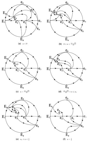
Figure 1. (a–p) Phase portraits on $z=0$.

Here, we focus on the cosmological solutions that have survived a sufficiently long epoch of matter dominance, followed by accelerated expansion. In the phase space, we need to search for saddle points with positive matter-density parameters and stable points that can exhibit accelerated expansion. The points involving matter points are $e_2$ and $e_5$, and only $e_4$ can be the accelerated point on the invariant plane $z=0$ in the model. Since the matter density parameter of $e_2$ exceeds the critical density of 1, we do not consider it as a matter point. The point $e_5$ is a saddle matter point when $1/2<\alpha <1$ and when $\alpha <(1-\sqrt{3})/2$ or $1/2<\alpha <1$ or $\alpha >(1+\sqrt{3})/2$, $e_4$ can be a stable accelerated point. For the limit $\left|\alpha \right|\to 0$ and 1, it can be found that under the limit $\left|\alpha \right|\to 0$, the point $e_4$ is not an accelerated point. When $\alpha \to 1^{+}$, the point $e_4$ is not an accelerated point, thus the trajectory from $e_5$ to $e_4$ is not a cosmological solution. The point $e_5$ is the saddle matter point and $e_4$ is a stable accelerated point when $\alpha \to 1^{-}$. Therefore, the trajectory from $e_5$ to $e_4$ can be a cosmological solution. The process from $e_5$ to $e_4$ can be regarded as a cosmological solution when $1/2<\alpha <3/4$, but there is no trajectory from $e_5$ to $e_4$ in this range. Therefore, the trajectory from $e_5$ to $e_4$ can be a cosmological solution when $3/4\le \alpha <1$, however $m_5=R{g}^{″}\left(R\right)/g^{\prime }\left(R\right)<0$ represents the divergence of the eigenvalues as $m_5\to 1^{-}$. This means that the system can not remain around the point $e_5$ for a long time. Thus, there are no viable cosmological solutions on the invariant plane $z=0$.

3.2. Phase Portraits on the Invariant Plane $y=0$ and Cosmological Solutions

On the invariant plane $y=0$ system (21) is

$$\begin{array}{cc}\hfill \frac{dx}{dN}& =-1+x^2-\frac{3}{2}z,\hfill \\ \hfill \frac{dy}{dN}& =z\left(x+\frac{5}{2}\right).\hfill \end{array}$$

(31)

System (31) has three equilibrium points, i.e., $e_1=(1,0)$, $e_2=(-1,0)$, and $e_3=(-5/2,7/2)$. Since the discussion of $e_1$ and $e_2$ has been presented above, we only discuss the point $e_3$ here. The point $e_3$ indicates ${\mathsf{\Omega }}^{\left(\mathrm{m}\right)}=0$ and ${\omega }^{\left(\mathrm{eff}\right)}=1/3$. Since radiation is not present in the model, this point does match any known matter and is not physically interesting. The eigenvalues are $-3/2$ and $-7/2$, thus $e_3$ is a stable node.

With the use of Poincaré compactification, we set $x=1/v$, $z=u/v$ on the local chart $U_1$. System (31) reads

$$\begin{array}{cc}\hfill \frac{du}{dN}& =uv\left(\frac{3}{2}u+v+\frac{5}{2}\right),\hfill \\ \hfill \frac{dv}{dN}& =v\left(\frac{3}{2}uv+v^2-1\right).\hfill \end{array}$$

(32)

As all the points of system (32) at infinity $v=0$ are equilibrium points, using the transformation $d{\tau }_1=vdN$, we rewrite this system

$$\begin{array}{cc}\hfill \frac{du}{d{\tau }_1}& =u\left(\frac{3}{2}u+v+\frac{5}{2}\right),\hfill \\ \hfill \frac{dv}{d{\tau }_1}& =\frac{3}{2}uv+v^2-1.\hfill \end{array}$$

(33)

However, none of the points at $v=0$ is the equilibrium point of system (33).

Similarly, we let $x=u/v$ and $z=1/v$ on the local chart $U_2$. Then, system (31) is

$$\begin{array}{cc}\hfill \frac{du}{dN}& =-v\left(\frac{5}{2}u+v+\frac{3}{2}\right),\hfill \\ \hfill \frac{dv}{dN}& =-v\left(u-\frac{5}{2}v\right).\hfill \end{array}$$

(34)

The origin $e_{10}=(0,0)$ is an equilibrium point of system (34). Although it has eigenvalues 0 and $3/2$, $e_{10}$ is not a semi-hyperbolic point as it is not an isolated singular point of system (34). Note that all the points on the axis $v=0$ are the equilibria of system (34) and there are no other equilibria on the axis $v=0$ if we remove the common factor v. In the region near $e_{10}$, $5u/2+v+3/2>0$, $du/dN<0$ for the positive semi-axis (PSA) of v illustrates that u decreases monotonously and $du/dN>0$ for the negative semi-axis (NSA) of v indicates that u increases monotonously. Above the straight line $u+5v/2=0$, $dv/dN<0$ for the PSA of v and $du/dN>0$ for the NSA of v. Below the straight line $u+5v/2=0$, $dv/dN>0$ for the PSA of v and $du/dN<0$ for the NSA of v. Therefore, we obtain the local phase portrait of $e_{10}$, which is shown in Figure 2. Since the points at infinity have negative values of the matter-density parameter, they can not be an epoch of the universe.

Figure 2. Local phase portrait of $e_{10}$.

We present the global phase portraits of system (31) on $y=0$ in Figure 3. None of the points on the invariant plane $y=0$ can show accelerated expansion, so we can not find a cosmological solution in Figure 3.

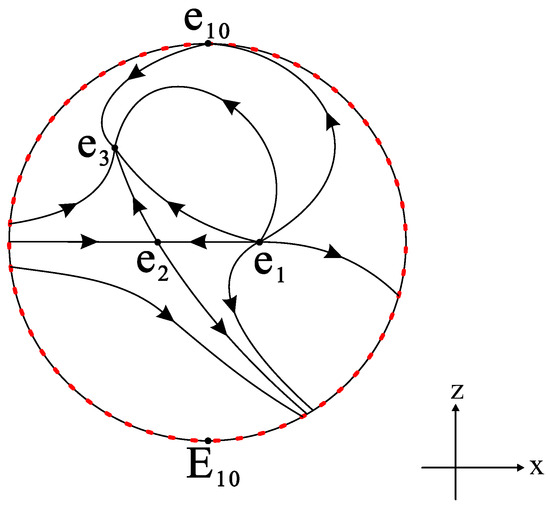
Figure 3. Phase portraits on $y=0$.

3.3. Phase Portraits on the Invariant Plane $1-x+(\alpha -1)y-z=0$ and Cosmological Solutions

On this invariant plane system (21) changes to the form

$$\begin{array}{cc}\hfill \frac{dy}{dN}& =y\left[(2\alpha -1)y+\frac{1}{\alpha -1}z+\frac{4\alpha -5}{\alpha -1}\right],\hfill \\ \hfill \frac{dz}{dN}& =z\left[(3\alpha -1)y-z+\frac{7}{2}\right].\hfill \end{array}$$

(35)

System (35) has four equilibrium points $e_1=(0,0)$, $e_3=(0,7/2)$, $e_4=((5-4\alpha )$/ $\left[\right(2\alpha -1\left)\right(\alpha -1\left)\right],0)$, and $e_6=((3-8\alpha )/\left(4{\alpha }^2\right),-\left[(2\alpha -3)(5\alpha -1)\right]/\left(4{\alpha }^2\right))$. According to the previous discussion, except for the point $e_6$, the physical meaning of other points is the same, but the mathematical stability may be different, so here we mainly discuss the point $e_6$. This point means ${\mathsf{\Omega }}^{\left(\mathrm{m}\right)}=0$ and ${\omega }^{\left(\mathrm{eff}\right)}=(1-2\alpha )/\left(2\alpha \right)$. It can display an accelerated-expansion era for $\alpha <0$ or $\alpha >3/4$. The eigenvalues of $e_6$ are given by $-\left[3(\alpha -1)(2\alpha +1)\pm \sqrt{(\alpha -1)(676{\alpha }^3-1328{\alpha }^2+573\alpha -81)}\right]/\left[8\alpha (\alpha -1)\right]$, it is a saddle when $\alpha <0$ or $0<\alpha <1/5$ or $3/8<\alpha <1$ or $\alpha >3/2$, it is a stable node when $1/5<\alpha <3/8$ or ${\alpha }_4\le \alpha <3/2$, a stable focus when $1<\alpha <{\alpha }_4$ and a saddle-node when $\alpha =1/5,3/8,3/2$. The constant ${\alpha }_4$ is the root of $676{\alpha }^3-1328{\alpha }^2+573\alpha -81=0$.

Applying the Poincaré compactification on the local chart $U_1$, we transform system (35) into

$$\begin{array}{cc}\hfill \frac{du}{dN}& =u\left[\frac{\alpha }{1-\alpha }u+\frac{3-\alpha }{2(\alpha -1)}+\alpha \right],\hfill \\ \hfill \frac{dv}{dN}& =v\left(\frac{1}{1-\alpha }u+\frac{4\alpha -5}{1-\alpha }v-2\alpha +1\right).\hfill \end{array}$$

(36)

At infinity $v=0$, system (36) has two equilibrium points, which are $e_{11}=(0,0)$ and $e_{12}=(\alpha -1,0)$. The equilibrium point $e_{11}$ has eigenvalues $\alpha$ and $1-2\alpha$, it is a saddle when $\alpha <0$ or $1/2<\alpha <1$ or $\alpha >1$, an unstable node when $0<\alpha <1/2$ and a saddle-node when $\alpha =1/2$. The equilibrium point $e_{12}$ has eigenvalues $-\alpha$ and $-2\alpha$, it is an unstable node when $\alpha <0$ and a stable node when $0<\alpha <1$ or $\alpha >1$.

On the local chart $U_2$, we use the Poincaré compactification again changing system (35) to

$$\begin{array}{cc}\hfill \frac{du}{dN}& =u\left[-\alpha u+\frac{\alpha -3}{2(\alpha -1)}v+\frac{\alpha }{\alpha -1}\right],\hfill \\ \hfill \frac{dv}{dN}& =v\left[(1-3\alpha )u-\frac{7}{2}v+1\right].\hfill \end{array}$$

(37)

The equilibrium point $e_{13}=(0,0)$ is the origin of system (37). This point has eigenvalues 1 and $\alpha /(\alpha -1)$, it is an unstable node when $\alpha <0$ or $\alpha >1$ and a saddle when $0<\alpha <1$.

For points $e_{11}$, $e_{12}$, and $e_{13}$ we all have ${\mathsf{\Omega }}^{\left(\mathrm{m}\right)}=0$. These points can be accelerated points when $\alpha <0$, however, they are not stable points in this range. Therefore, these three infinite points are not included in the cosmological solutions.

Since the stabilities of these four finite equilibrium points ($e_1$, $e_3$, $e_4$, and $e_6$) and three infinite equilibrium points ($e_{11}$, $e_{12}$, and $e_{13}$) are different when $\alpha$ changes, we make a summary in Table 4. Moreover, we present the global phase portraits of system (35) on $1-x+(\alpha -1)y-z=0$ in Figure 4. On the invariant plane $1-x+(\alpha -1)y-z=0$, the matter-density parameters are zero at all the equilibrium points. Since we can not find any matter points, there is no cosmological solution in Figure 4.

Table 4. Equilibrium points and their types for different values of $\alpha$ of system (35).

Values of $\mathit{\alpha }$	Finite Equilibrium Points	Infinite Equilibrium Points
$\alpha <0$	$e_1$ is an unstable node, $e_3$ and $e_6$ are saddles, $e_4$ is a stable node	$e_{11}$ is a saddle, $e_{12}$ and $e_{13}$ are unstable nodes
$0<\alpha <\frac{1}{5}$	$e_1$ is an unstable node, $e_3$ and $e_6$ are saddles, $e_4$ is a stable node	$e_{11}$ is an unstable node, $e_{12}$ is a stable node, $e_{13}$ is a saddle
$\alpha =\frac{1}{5}$	$e_1$ is an unstable node, $e_3$ is a saddle, $e_4$ and $e_6$ are saddle-nodes	$e_{11}$ is an unstable node, $e_{12}$ is a stable node, $e_{13}$ is a saddle
$\frac{1}{5}<\alpha <\frac{3}{8}$	$e_1$ is an unstable node, $e_3$ and $e_4$ are saddles, $e_6$ is a stable node	$e_{11}$ is an unstable node, $e_{12}$ is a stable node, $e_{13}$ is a saddle
$\alpha =\frac{3}{8}$	$e_1$ is an unstable node, $e_3$ and $e_6$ are saddle-nodes, $e_4$ is a saddle	$e_{11}$ is an unstable node, $e_{12}$ is a stable node, $e_{13}$ is a saddle
$\frac{3}{8}<\alpha <\frac{1}{2}$	$e_1$ is an unstable node, $e_3$ is a stable node, $e_4$ and $e_6$ are saddles	$e_{11}$ is an unstable node, $e_{12}$ is a stable node, $e_{13}$ is a saddle
$\alpha =\frac{1}{2}$	$e_1$ is an unstable node, $e_3$ is a stable node, $e_6$ is a saddle	$e_{11}$ is a saddle-node, $e_{12}$ is a stable node, $e_{13}$ is a saddle
$\frac{1}{2}<\alpha <1$	$e_1$ is an unstable node, $e_3$ and $e_4$ are stable nodes, $e_6$ is a saddle	$e_{11}$ and $e_{13}$ are saddles, $e_{12}$ is a stable node
$1<\alpha <\frac{5}{4}$	$e_1$ and $e_3$ are saddles, $e_4$ is an unstable node, $e_6$ is a stable focus	$e_{11}$ is a saddle, $e_{12}$ is a stable node, $e_{13}$ is an unstable node
$\alpha =\frac{5}{4}$	$e_1$ and $e_4$ are saddle-nodes, $e_3$ is a saddle, $e_6$ is a stable focus	$e_{11}$ is a saddle, $e_{12}$ is a stable node, $e_{13}$ is an unstable node
$\frac{5}{4}<\alpha <{\alpha }_4$	$e_1$ is an unstable node, $e_3$ and $e_4$ are saddles, $e_6$ is a stable focus	$e_{11}$ is a saddle, $e_{12}$ is a stable node, $e_{13}$ is an unstable node
${\alpha }_4\le \alpha <\frac{3}{2}$	$e_1$ is an unstable node, $e_3$ and $e_4$ are saddles, $e_6$ is a stable node	$e_{11}$ is a saddle, $e_{12}$ is a stable node, $e_{13}$ is an unstable node
$\alpha =\frac{3}{2}$	$e_1$ is an unstable node, $e_3$ is a saddle, $e_4$ and $e_6$ are saddle-nodes	$e_{11}$ is a saddle, $e_{12}$ is a stable node, $e_{13}$ is an unstable node
$\alpha >\frac{3}{2}$	$e_1$ is an unstable node, $e_3$ and $e_6$ are saddles, $e_4$ is a stable node	$e_{11}$ is a saddle, $e_{12}$ is a stable node, $e_{13}$ is an unstable node

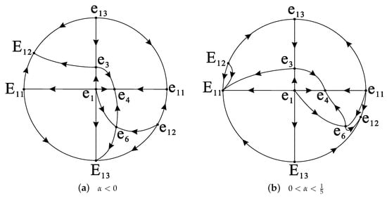
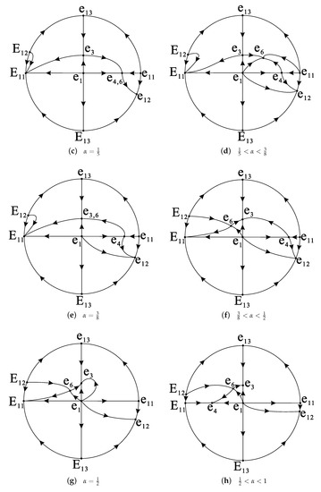
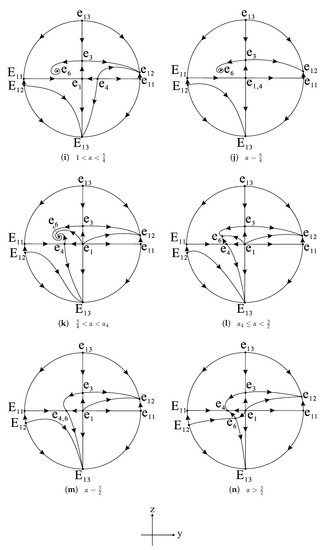
Figure 4. (a–n) Phase portraits on $1-x+(\alpha -1)y-z=0$.

3.4. Equilibrium Points on the Poincaré Sphere at Infinity

Using the 3D Poincaré compactification [49,53], we let $x=1/z_3$, $y=z_1/z_3$, $z=z_2/z_3$ on the local chart $U_1$ and then system (21) becomes

$$\begin{array}{cc}\hfill \frac{d{z}_1}{dN}& =z_1\left[(3-\alpha )z_1{z}_3+\frac{3}{2}{z}_2{z}_3+z_3^2+\alpha z_1+4z_3-\frac{\alpha }{\alpha -1}\right],\hfill \\ \hfill \frac{d{z}_2}{dN}& =z_2\left[(3-\alpha )z_1{z}_3+\frac{3}{2}{z}_2{z}_3+z_3^2+\alpha z_1+\frac{5}{2}{z}_3\right],\hfill \\ \hfill \frac{d{z}_3}{dN}& =z_3\left[(3-\alpha )z_1{z}_3+\frac{3}{2}{z}_2{z}_3+z_3^2-\alpha z_1-1\right].\hfill \end{array}$$

(38)

As $z_3=0$ corresponds to the infinity, we only need to study equilibrium points with $z_3=0$ on the different local chart of Poincaré sphere. System (38) has equilibrium points $p_7=(1/(\alpha -1),0,0)$ and $(0,z_2,0)$ for all $z_2\in \mathbb{R}$ when $z_3=0$. The equilibrium point $P_7$ has eigenvalues $(2\alpha -1)/(1-\alpha )$, $\alpha /(\alpha -1)$ and $\alpha /(\alpha -1)$, it is a stable node when $0<\alpha <1/2$ and it is a saddle when $\alpha <0$ or $1/2<\alpha <1$ or $\alpha >1$. The equilibrium point $(0,z_2,0)$ has eigenvalues $-1$, 0, and $\alpha /(1-\alpha )$. Applying the normally hyperbolic sub-manifold theorem [54], the equilibrium point $(0,z_2,0)$ has a two-dimensional stable manifold when $\alpha <0$ or $\alpha >1$ and when $0<\alpha <1$, it has a one-dimensional unstable manifold and a one-dimensional stable manifold.

Similar to the local chart $U_1$, we set $x=z_1/z_3$, $y=1/z_3$, $z=z_2/z_3$ on $U_2$. we obtain

$$\begin{array}{cc}\hfill \frac{d{z}_1}{dN}& =\frac{\alpha }{\alpha -1}{z}_1^2-4z_1{z}_3-\frac{3}{2}{z}_2{z}_3-z_3^2-\alpha z_1+(\alpha -3)z_3,\hfill \\ \hfill \frac{d{z}_2}{dN}& =z_2\left(\frac{\alpha }{\alpha -1}{z}_1-\frac{3}{2}{z}_3\right),\hfill \\ \hfill \frac{d{z}_3}{dN}& =z_3\left(\frac{1}{\alpha -1}{z}_1-4z_3-2\alpha \right).\hfill \end{array}$$

(39)

System (39) has an equilibrium point $p_9=(\alpha -1,0,0)$ when $z_2=0$ and $z_3=0$. The equilibrium point $p_9$ has eigenvalues $\alpha$, $\alpha$, and $1-2\alpha$, it is an unstable node when $0<\alpha <1/2$ and it is a saddle when $\alpha <0$ or $1/2<\alpha <1$ or $\alpha >1$. Since other infinite equilibrium points of system (39) are contained in the local chart $U_1$, we will not analyze them.

Similarly, we have $x=z_1/z_3$, $y=z_2/z_3$, and $z=1/z_3$ on the local chart $U_3$ and then system (21) is

$$\begin{array}{cc}\hfill \frac{d{z}_1}{dN}& =-\alpha z_1{z}_2-\frac{5}{2}{z}_1{z}_3+(\alpha -3)z_2{z}_3-z_3^2-\frac{3}{2}{z}_3,\hfill \\ \hfill \frac{d{z}_2}{dN}& =z_2\left(\frac{\alpha }{1-\alpha }{z}_1+\frac{3}{2}{z}_3\right),\hfill \\ \hfill \frac{d{z}_3}{dN}& =z_3\left(-z_1{z}_3-2\alpha z_2-\frac{5}{2}z\right).\hfill \end{array}$$

(40)

The origin $p_{10}=(0,0,0)$ of system (40) is an equilibrium point. In the local chart $U_3$, we will not study other equilibria of system (40) expect $p_{10}$ because they have been discussed on the local charts $U_1$ and $U_2$. We take $z_3=0$ and system (40) becomes

$$\begin{array}{cc}\hfill \frac{d{z}_1}{dN}& =-\alpha z_1{z}_2,\hfill \\ \hfill \frac{d{z}_2}{dN}& =-\frac{\alpha }{\alpha -1}{z}_1{z}_2.\hfill \end{array}$$

(41)

Obviously, we can obtain $z_1=(\alpha -1)z_2+C_1$, where $C_1$ is a constant. As $z_1$ is linearly related to $z_2$, the equilibrium point $p_{10}$ is an unstable center when $\alpha >1$ and a stable center when $\alpha <0$ or $0<\alpha <1/2$ or $1/2<\alpha <1$.

Obviously, we can obtain $z_1=(-1/2)z_2+C_2$, where $C_2$ is a constant. As $z_1$ is linearly related to $z_2$, the equilibrium point $q_9$ is a stable center.

4. The Case $\left|\mathbf{\alpha }\right|\to \mathbf{1}$ in 3D

According to Ref. [41], the best solution of this model can be achieved for $\alpha$ tending to one. Therefore, we present global phase of system (21) on three invariant planes when $\left|\alpha \right|\to 1$ in Figure 5 and Figure 6, where $CS$ represents the cosmological solution.

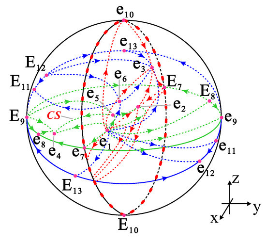
Figure 5. Phase portraits of system (21) on three invariant planes when $\alpha \to 1^{-}$.

Figure 6. Phase portraits of system (21) on three invariant planes when $\alpha \to 1^{+}$.

When $\alpha \to 1^{-}$, there is only one saddle matter point $e_5$ and one stable accelerated point $e_4$. The trajectory from $e_5$ to $e_4$ on the invariant plane $z=0$ can be considered as a cosmological solution. However, this case approximates GR because $z=0$ leads to $h\left(T\right)=0$. Note that GR can not explain the late-time behavior of the universe. This cosmological solution is unacceptable.

When $\alpha \to 1^{+}$, $e_4$ is not an accelerated point, and $e_6$ is the only stable accelerated point instead. There is only one saddle matter point $e_5$. We can not find a cosmological solution on three invariant planes because the accelerated point $e_6$ and the matter saddle point $e_5$ are not on the same plane. However, by analyzing the trajectories around these three points in 3D, we find that the saddle matter point $e_5$ can reach the stable accelerated point $e_6$, which is an acceptable cosmological solution. This solution from $e_5$ to $e_6$ corresponds to the solution from $P_3$ to $P_1$ obtained in Ref. [41].

5. The Form $\mathit{g}\left(\mathit{R}\right)=\mathit{R}+\mathbf{\xi }{\mathit{R}}^{\mathbf{\alpha }}$

In this section, we briefly discuss a case that is considered to be more interesting and physical when $f(R,T)=R+\xi R^{\alpha }+\zeta \sqrt{-T}$. Considering a spatially flat FLRW metric and the model’s later-time behaviors. This theory gives

$$\begin{array}{cc}\hfill 1+& \frac{R+\xi R^{\alpha }}{6H^2(1+\xi \alpha R^{\alpha -1})}+\frac{\zeta \sqrt{-T}}{6H^2(1+\xi \alpha R^{\alpha -1})}-\frac{R}{6H^2}+\frac{{\dot{g}}^{\prime }}{H(1+\xi \alpha R^{\alpha -1})}\hfill \\ \hfill & =\frac{8\pi G{\rho }^{\left(\mathrm{m}\right)}}{3H^2(1+\xi \alpha R^{\alpha -1})}-\frac{\zeta {\rho }^{\left(\mathrm{m}\right)}}{6H^2\sqrt{-T}(1+\xi \alpha R^{\alpha -1})},\hfill \end{array}$$

(42)

and

$$\begin{array}{cc}\hfill 2\frac{\dot{H}}{H^2}+& \frac{{\ddot{g}}^{\prime }}{H^2(1+\xi \alpha R^{\alpha -1})}-\frac{{\dot{g}}^{\prime }}{H(1+\xi \alpha R^{\alpha -1})}\hfill \\ \hfill =& -\frac{8\pi G{\rho }^{\left(\mathrm{m}\right)}}{H^2(1+\xi \alpha R^{\alpha -1})}+\frac{\zeta {\rho }^{\left(\mathrm{m}\right)}}{2\sqrt{-T}{H}^2(1+\xi \alpha R^{\alpha -1})},\hfill \end{array}$$

(43)

as the Friedmann-like equation and Raychaudhuri-like equation, respectively. The dynamical system becomes

$$\begin{array}{cc}\hfill \frac{d{x}_1}{dN}& =x_1(x_1-x_3)-3x_2-x_3-\frac{3}{2}{x}_4-1,\hfill \\ \hfill \frac{d{x}_2}{dN}& =\frac{x_1{x}_3}{m}+x_2(x_1-2x_3+4),\hfill \\ \hfill \frac{d{x}_3}{dN}& =-\frac{x_1{x}_3}{m}+2x_3(2-x_3),\hfill \\ \hfill \frac{d{x}_4}{dN}& =x_4\left(x_1-2x_3+\frac{5}{2}\right).\hfill \end{array}$$

(44)

The density parameter of matter ${\mathsf{\Omega }}^{\left(\mathrm{m}\right)}$ and effective equation of state ${\omega }^{\left(\mathrm{eff}\right)}$ read as follows

$${\mathsf{\Omega }}^{\left(\mathrm{m}\right)}=1-x_1-x_2-x_3-x_4,$$

(45)

$${\omega }^{\left(\mathrm{eff}\right)}=\frac{1}{3}(1-2x_3).$$

(46)

The equilibrium points of system (44) and the related eigenvalues are listed in Table 5 and Table 6, respectively. Furthermore, the parameter $r=r(x_2,x_3)$ satisfies

$$\frac{dr}{dN}=\frac{\partial r(x_2,x_3)}{\partial x_2}\frac{d{x}_2}{dN}+\frac{\partial r(x_2,x_3)}{\partial x_3}\frac{d{x}_3}{dN}=0.$$

(47)

Table 5. Equilibrium points of system (44).

Equilibrium Points	Coordinates $(\mathit{x},\mathit{y},\mathit{z})$	${\mathsf{\Omega }}^{\left(\mathbf{m}\right)}$	${\mathit{\omega }}^{\left(\mathbf{eff}\right)}$
$q_1$	($1,0,0,0$)	0	$\frac{1}{3}$
$q_2$	($-1,0,0,0$)	2	$\frac{1}{3}$
$q_3$	($-\frac{5}{2},0,0,\frac{7}{2}$)	0	$\frac{1}{3}$
$q_4$	($-4,5,0,0$)	0	$\frac{1}{3}$
$q_5$	($0,-1,2,0$)	0	$-1$
$q_6$	($\frac{3m}{m+1},-\frac{4m+1}{2{(1+m)}^2},\frac{4m+1}{2(m+1)},0$)	$\frac{2-3m-8m^2}{2{(m+1)}^2}$	$-\frac{m}{m+1}$
$q_7$	($\frac{2(1-m)}{2m+1},\frac{1-4m}{m(2m+1)},-\frac{(1-4m)(m+1)}{m(2m+1)}$)	0	$\frac{2-5m-6m^2}{3m(2m+1)}$
$q_8$	($\frac{3m}{2(m+1)},-\frac{8m+5}{4{(m+1)}^2},\frac{8m+5}{4(m+1)},\frac{4-3m-10m^2}{4{(m+1)}^2}$)	0	$-\frac{2m+1}{2(m+1)}$

Table 6. Eigenvalues of equilibrium points.

Equilibrium Points	Eigenvalues
$q_1$	$\frac{7}{2},2,\frac{m(9m-1)+r(r+1)m^{\prime }\pm a(m,m^{\prime })}{2m^2}$
$q_2$	$-2,\frac{3}{2},\frac{m(7m+1)-r(r+1)m^{\prime }\pm a(m,m^{\prime })}{2m^2}$
$q_3$	$-\frac{7}{2},-\frac{3}{2},\frac{m(11m+5)-r(r+1)m^{\prime }\pm 5a(m,m^{\prime })}{4m^2}$
$q_4$	$-5,-3,4(1+\frac{1}{m}),-\frac{3}{2}$
$q_5$	$-3,-\frac{3}{2},-\frac{3}{2}\pm \sqrt{\frac{25}{4}-\frac{4}{m}}$
$q_6$	$\frac{3}{2},\frac{-3m\pm b\left(m\right)}{4m(m+1)},3(1+m^{\prime })$
$q_7$	$-4+\frac{1}{m},\frac{-8m^2-3m+2}{m(2m+1)},\frac{2(1-m^2)(1+m^{\prime })}{m(2m+1)},\frac{-10m^2-3m+4}{2m(2m+1)}$
$q_8$	$-\frac{3}{2},\frac{-3m(m+1)(2m+3)\pm c\left(m\right)}{8m{(m+1)}^2},\frac{3}{2}(1+m^{\prime })$

Note: a(m,m′) = {m²(m + 1)² + rm′[−2m(m + 1) + 2(m − 1)mr + r(1 + r²)m′]}^1/2, b(m) ≡ [m(256m³ + 160m² − 31m − 16)]^1/2, c(m) ≡ {m(m + 1)²[m(676m² + 700m − 55) − 160]}^1/2.

Using Equations (13)–(15), Equation (47) can be rewritten as

$$\frac{dr}{dN}=r\left(\frac{1+r+m\left(r\right)}{m\left(r\right)}\right)x_1=0,$$

(48)

where $m\left(r\right)=\alpha (r+1)/r$. Let

$$M\left(r\right)\equiv \frac{1+r+m\left(r\right)}{m\left(r\right)},$$

(49)

which is well-defined for $m\left(r\right)\ne 0$ as all solutions that hold $m\left(r\right)=-r-1$ must satisfy $M\left(r\right)=0$. Therefore, an acceptable solution must satisfy $r=0$ or $M\left(r\right)=0$ or $x_1=0$. By assuming $r\ne -1$ in Equation (49), we obtain $M\left(r\right)=1+r/\alpha$, which gives $M(r=-1)=1-1/\alpha$. The condition $M\left(r\right)=0$ is true only when $r=-\alpha$, resulting in $m\ne 0$. On the other hand, the point $q_6$ is the matter point when $r=-1$. Note that models with $\alpha =1$ can be acceptable, we mainly discuss the case of $\alpha \to 1$ where $M(r=-1)\approx 0$.

When $\alpha \to 1^{-}$, as $r=-\alpha$, we can obtain $r\to -1^{+}$, which means $m\left(r\right)\to 0^{+}$. Within this range, the eigenvalues of point $q_6$ can be approximated as

$$\frac{3}{2},3(1+m^{\prime }),-\frac{3}{4}\pm \sqrt{-\frac{1}{m}}.$$

(50)

This point is a matter saddle point with ${\mathsf{\Omega }}^{\left(\mathrm{m}\right)}=1$ and ${\omega }^{\left(\mathrm{eff}\right)}=0$. The point $q_8$ is a stable accelerated point for $m_{q_8}^{\prime }<-1$. Therefore, the transition from $q_6$ to $q_8$ is viable for leaving the matter-dominated era with $m_{q_6}^{\prime }>-1$ and entering the accelerated epoch $m_{q_8}^{\prime }<-1$. Moreover, the transition from $q_6$ to $q_5$ is possible. For $m(r=-2)=\alpha /2$, the de Sitter point $q_5$ is an acceptable final attractor for the cosmological solutions. When $m_{q_6}^{\prime }>-1$, the trajectories can reach the final attractor $q_5$ after leaving the matter point $q_6$.

When $\alpha \to 1^{+}$, we obtain the limit $m\left(r\right)\to 0^{-}$. The point $q_6$ is not acceptable in this range because there are two eigenvalues approaching infinity. This indicates the matter-dominated era is short and does not match with the observational data. Since there are no other matter points, we cannot find the cosmological solution withinn this limit.

6. Conclusions

The dynamics of the $f(R,T)$ gravity model on the invariant planes for a perfect fluid in a spatially flat FLRW metric are studied with the form $g\left(R\right)+h\left(T\right)$. By considering the conservation of the energy–momentum tensor, it has been presented that the functionality of $h\left(T\right)$ must have the form $h\left(T\right)=C\sqrt{T}$ in the minimal models. More precisely, we mainly analyze the model in the type of $\xi R^{\alpha }+\zeta \sqrt{-T}$. We apply two powerful dynamic analysis tools, singularity theory, and Poincaré compactification. Using the singularity theory, we can understand the direction of trajectories near some unusual equilibrium points, such as saddle-nodes. The infinite phase space can be transformed into a finite space with the application of Poincaré compactification. Through the use of these two techniques, the stability of all the equilibrium points and global phase on the invariant planes is presented. Finally, we discussed the case of $\left|\alpha \right|\to 1$. All cosmological solutions have been marked in the figures.

Since the parameter $\alpha$ in this paper has a wider range of values, in order to accurately show the evolution of the model on three invariant planes simultaneously in space, we finally selected the limit $\left|\alpha \right|\to 1$, which visually illustrates the dynamic behavior of the model at this limit. The trajectory from $e_5$ to $e_4$ on the invariant plane $z=0$ is not the desired cosmological solution when $\alpha \to 1^{-}$, and since this case approaches GR and we adopt it. When $\alpha \to 1^{+}$, we have a stable accelerated point $e_6$, and two saddle matter points $e_2$ and $e_5$. Although there are no cosmological solutions on the three invariant planes, by analyzing the trajectories around these three points, we find the trajectories from $e_5$ to $e_6$ exist, which can be considered as a cosmological solution. Furthermore, this solution is consistent with the cosmological solution from $P_3$ to $P_4$ in Ref. [41]. In addition, we briefly discuss a more interesting and physical form $f(R,T)=R+\xi R^{\alpha }+\zeta \sqrt{-T}$, and find two viable cosmological solutions $q_6$ to $q_5$ and $q_6$ to $q_8$ when $\alpha \to 1^{-}$.

References

- Will, C.M.; Anderson, J.L. Theory and experiment in gravitational physics. Am. J. Phys. 1994, 62, 1153. [Google Scholar] [CrossRef]
- Turyshev, S.G. Experimental tests of general relativity: Recent progress and future directions. Physics-Uspekhi 2009, 52, 1. [Google Scholar] [CrossRef] [Green Version]
- Iorio, L.; Lichteneggrr, H.I.M.; Ruggiero, M.L.; Corda, C. Phenomenology of the Lense-Thirring effect in the solar system. Astrophys. Space. Sci. 2011, 331, 351–395. [Google Scholar] [CrossRef] [Green Version]
- Peeebles, P.J.E. Testing general relativity on the scales of cosmology. arXiv 2004, arXiv:astro-ph/0410284. [Google Scholar]
- Bennett, C.L.; Bay, M.; Halpern, M.; Hinshaw, G.; Jackson, C.; Jarosik, N.; Kogut, A.; Limon, M.; Meyer, S.S.; Page, L.; et al. The microwave anisotropy probe* mission. Astrophys. J. 2003, 583, 1. [Google Scholar] [CrossRef] [Green Version]
- Farajollahi, H.; Farhoudi, M.; Shojaie, H. On dynamics of Brans–Dicke theory of gravitation. Int. J. Theor. Phys. 2010, 49, 2558–2568. [Google Scholar] [CrossRef] [Green Version]
- Bahrehbakhsh, A.F.; Farhoudi, M.; Shojaie, H. FRW cosmology from five dimensional vacuum Brans–Dicke theory. Gen. Relativ. Gravit. 2011, 43, 847–869. [Google Scholar] [CrossRef] [Green Version]
- De Felice, A.; Tsujikawa, S. f(R) Theories. Living. Rev. Relativ. 2010, 13, 3. [Google Scholar] [CrossRef] [Green Version]
- Capozziello, S.; De Laurentis, M. Extended theories of gravity. Phys. Rep. 2011, 509, 167–321. [Google Scholar] [CrossRef] [Green Version]
- Nojiri, S.; Odintsov, S.D.; Mittal, A. Unified cosmic history in modified gravity: From f(R) theory to Lorentz non-invariant models. Phys. Rep. 2011, 505, 59–144. [Google Scholar] [CrossRef] [Green Version]
- Starobinsky, A.A. Disappearing cosmological constant in f(R) gravity. JETP. Lett. 2007, 86, 157–163. [Google Scholar] [CrossRef] [Green Version]
- Tsujikawa, S. Observational signatures of f(R) dark energy models that satisfy cosmological and local gravity constraints. Phys. Rev. D Part. Fields. 2007, 77, 315–317. [Google Scholar] [CrossRef] [Green Version]
- Nojiri, S.; Odintsov, S.D.; Sáez-Gómez, D. Cosmological reconstruction of realistic modified f(R) gravities. Phys. Lett. B 2009, 681, 74–80. [Google Scholar] [CrossRef] [Green Version]
- Nojiri, S.; Odintsov, S.D.; Oikonomou, V.K. Unifying inflation with early and late-time dark energy in f(R) gravity. Phys. Dark Universe 2020, 29, 100602. [Google Scholar] [CrossRef]
- Hu, W.; Sawicki, I. Models of f(R) cosmic acceleration that evade solar-system tests. Astrophys. Space Sci. 2007, 76, 064004. [Google Scholar] [CrossRef] [Green Version]
- Bergliaffa, S.E.P. Constraining f(R) theories with the energy conditions. New Astron. 2006, 642, 311–314. [Google Scholar]
- Santos, J.; Alcaniz, J.S.; Reboucas, M.J.; Carvalho, F.C. Energy conditions in f(R) gravity. Phys. Rev. D 2007, 76, 083513. [Google Scholar] [CrossRef] [Green Version]
- Amendola, L.; Tsujikawa, S. Phantom crossing, equation-of-state singularities, and local gravity constraints in f(R) models. Phys. Lett. B 2008, 660, 125–132. [Google Scholar] [CrossRef] [Green Version]
- Pan, Y.; He, Y.; Qi, J.Z.; Li, J.; Cao, S.; Liu, T.H.; Wang, J. Testing f(R) gravity with the simulated data of gravitational waves from the Einstein Telescope. Astrophys. J. 2021, 911, 135. [Google Scholar] [CrossRef]
- Bertolami, O.; Boehmer, C.G.; Harko, T.; Lobo, F.S.N. Extra force in f(R) modified theories of gravity. Phys. Rev. D 2007, 75, 104016. [Google Scholar] [CrossRef] [Green Version]
- Harko, T. Modified gravity with arbitrary coupling between matter and geometry. Phys. Lett. B 2008, 669, 376–379. [Google Scholar] [CrossRef] [Green Version]
- Harko, T.; Lobo, F.S.N. f(R,Lm) gravity. Eur. Phys. J. C 2010, 70, 373–379. [Google Scholar] [CrossRef]
- Harko, T.; Lobo, F.S.N.; Nojiri, S.; Odintsov, S.D. f(R,T) gravity. Appl. Math. Nonlinear Sci. 2011, 84, 024020. [Google Scholar] [CrossRef] [Green Version]
- Sun, G.; Huang, Y.C. The cosmology in f(R,τ) gravity without dark energy. Int. J. Mod. Phys. D 2016, 25, 1650038. [Google Scholar] [CrossRef] [Green Version]
- Zaregonbadi, R.; Farhoudi, M.; Riazi, N. Dark matter from f(R,T) gravity. Phys. Rev. D 2016, 94, 084052. [Google Scholar] [CrossRef] [Green Version]
- Bhattacharjee, S.; Sahoo, P.K. Redshift drift in f(R,T) gravity. New Astron. 2020, 81, 101425. [Google Scholar] [CrossRef]
- Moraes, P.H.R.S.; Sahoo, P.K. Nonexotic matter wormholes in a trace of the energy-momentum tensor squared gravity. Phys. Rev. D 2018, 57, 024007. [Google Scholar] [CrossRef] [Green Version]
- Bhatti, M.Z.; Yousaf, Z.; Ilyas, M. Existence of wormhole solutions and energy conditions in f(R,T) gravity. J. Astrophys. 2018, 39, 1–11. [Google Scholar] [CrossRef]
- Sharif, M.; Zubair, M. Thermodynamics in f(R,T) theory of gravity. J. Cosmol. Astropart. Phys. 2012, 2012, 028. [Google Scholar] [CrossRef] [Green Version]
- Houndjo, M.J.S.; Alvarenga, F.G.; Rodrigues, M.E.; Jardim, D.F.; Myrzakulov, R. Thermodynamics in Little Rip cosmology in the framework of a type of f(R,T) gravity. Eur. Phys. J. Plus 2014, 129, 1–12. [Google Scholar] [CrossRef] [Green Version]
- Bhattacharjee, S.; Sahoo, P.K. Comprehensive analysis of a non-singular bounce in f(R,T) gravitation. Phys. Dark Universe 2020, 28, 100537. [Google Scholar] [CrossRef] [Green Version]
- Sahoo, P.; Bhattacharjee, S.; Tripathy, S.K.; Sahoo, P.K. Bouncing scenario in f(R,T) gravity. Mod. Phys. Lett. A 2020, 35, 2050095. [Google Scholar] [CrossRef]
- Sahoo, P.K.; Bhattacharjee, S. Gravitational baryogenesis in non-minimal coupled f(R,T) gravity. Int. J. Theor. Phys. 2020, 59, 1451–1459. [Google Scholar] [CrossRef] [Green Version]
- Alvarenga, F.G.; De La Cruz-Dombriz, A.; Houndjo, M.J.S.; Rodrigues, M.E.; Sáez-Gómez, D. Dynamics of scalar perturbations in f(R,T) gravity. Phys. Rev. D 2013, 87, 103526. [Google Scholar] [CrossRef] [Green Version]
- Alves, M.E.S.; Moraes, P.H.R.S.; De Araujo, J.C.N.; Malheiro, M. Gravitational waves in f(R,T) and f(R,Tϕ) theories of gravity. Phys. Rev. D 2016, 94, 024032. [Google Scholar] [CrossRef] [Green Version]
- Sharif, M.; Siddiqa, A. Propagation of polar gravitational waves in f(R,T) scenario. Gen. Relativ. Gravit. 2019, 51, 74. [Google Scholar] [CrossRef] [Green Version]
- Houndjo, M.J.S. Reconstruction of f(R,T) gravity describing matter dominated and accelerated phases. Int. J. Mod. Phys. D 2012, 21, 1250003. [Google Scholar] [CrossRef] [Green Version]
- Sharif, M.; Zubair, M. Cosmological reconstruction and stability in f(R,T) gravity. Gen. Relativ. Gravit. 2014, 46, 1723. [Google Scholar] [CrossRef]
- Singh, C.P.; Singh, V. Reconstruction of modified f(R,T) gravity with perfect fluid cosmological models. Gen. Relativ. Gravit. 2014, 46, 1696. [Google Scholar] [CrossRef]
- Shabani, H.; Farhoudi, M. Cosmological and solar system consequences of f(R,T) gravity models. Phys. Rev. D 2014, 90, 044031. [Google Scholar] [CrossRef] [Green Version]
- Shabani, H.; Farhoudi, M. f(R,T) cosmological models in phase space. Phys. Rev. D 2013, 88, 044048. [Google Scholar] [CrossRef] [Green Version]
- Baffou, E.H.; Kpadonou, A.V.; Rodrigues, M.E.; Houndjo, M.J.S.; Tossa, J. Cosmological viable f(R,T) dark energy model: Dynamics and stability. Astrophys. Space. Sci. 2015, 356, 173–180. [Google Scholar] [CrossRef] [Green Version]
- Sharma, U.K.; Pradhan, A. Propagation of polar gravitational waves in f(R,T) scenario. Int. J. Geom. Methods Mod. Phys. 2018, 15, 1850014. [Google Scholar] [CrossRef]
- Abchouyeh, M.A.; Mirza, B.; Shahidi, P.; Oboudiat, F. Late time dynamics of f(R,T,RμνTμν) gravity. Int. J. Geom. Methods Mod. Phys. 2020, 17, 2050008. [Google Scholar] [CrossRef] [Green Version]
- Gonçalves, T.B.; Rosa, J.L.; Lobo, F.S.N. Cosmology in the novel scalar-tensor representation of f(R,T) gravity. arXiv 2021, arXiv:2112.03652. [Google Scholar]
- Santos, A.F. Gödel solution in f(R,T) gravity. Mod. Phys. Lett. A 2013, 28, 1350141. [Google Scholar] [CrossRef] [Green Version]
- Guo, J.Q.; Frolov, A.V. Cosmological dynamics in f(R) dravity. Phys. Rev. D 2013, 88, 124036. [Google Scholar] [CrossRef] [Green Version]
- Zonunmawia, H.; Khyllep, W.; Dutta, J.; Järv, L. Cosmological dynamics of brane gravity: A grobal dynamical system perspective. Phys. Rev. D 2018, 98, 083532. [Google Scholar] [CrossRef] [Green Version]
- Gao, F.B.; Llibre, J. Global dynamics of the Hořava-Lifshitz cosmological model in a non-flat universe with non-zero cosmological constant. Universe 2021, 7, 445. [Google Scholar] [CrossRef]
- Singh, A.; Singh, G.P.; Pradhan, A. Cosmic dynamics and qualitative study of Rastall model with spatial curvature. arXiv 2022, arXiv:2205.13934. [Google Scholar] [CrossRef]
- Amendola, L. Coupled quintessence. Phys. Rev. D 2000, 62, 043511. [Google Scholar] [CrossRef] [Green Version]
- Dumortier, F.; Llibre, J.; Ateés, J.C. Qualitative Theory of Planar Differential Syetems; Springer: Berlin/Heidelberg, Germany, 2006. [Google Scholar]
- Cima, A.; Llibre, J. Bounded polynomial vector fields. Trans. Am. Math. Soc. 1990, 318, 557–579. [Google Scholar] [CrossRef]
- Álvarez, M.J.; Pugh, C.C.; Shub, M. Invariant Manifolds; Springer: Berlin/Heidelberg, Germany, 1977. [Google Scholar]
Publisher’s Note: MDPI stays neutral with regard to jurisdictional claims in published maps and institutional affiliations. |
© 2022 by the authors. Licensee MDPI, Basel, Switzerland. This article is an open access article distributed under the terms and conditions of the Creative Commons Attribution (CC BY) license (https://creativecommons.org/licenses/by/4.0/).