Non-Static Fluid Spheres Admitting a Conformal Killing Vector: Exact Solutions

Abstract

We carry on a general study on non-static spherically symmetric fluids admitting a conformal Killing vector (CKV). Several families of exact analytical solutions are found for different choices of the CKV in both the dissipative and the adiabatic regime. To specify the solutions, besides the fulfillment of the junction conditions on the boundary of the fluid distribution, different conditions are imposed, such as a vanishing complexity factor and quasi-homologous evolution. A detailed analysis of the obtained solutions and its prospective applications to astrophysical scenarios, as well as alternative approaches to obtain new solutions, are discussed.

1. Introduction

The purpose of this work is twofold. On the one hand, we want to delve deeper into the physical consequences derived from the assumption that a given space–time admits a CKV. This interest, in turn, is motivated by the relevance of such a kind of symmetry in hydrodynamics.

Indeed, in general relativity, self-similar solutions are related to the existence of a homothetic Killing vector field (HKV), a generalization of which is a conformal Killing vector field (CKV). The physical interest of systems admitting a CKV is then suggested by the important role played by self-similarity in classical hydrodynamics.

Thus, in Newtonian hydrodynamics, self-similar solutions are those described by means of physical quantities that are functions depending on dimensionless variables $x/l\left(t\right)$, where x and t are independent space and time variables and l is a time-dependent scale. Therefore, the spatial distribution of the characteristics of motion remains similar to itself at all times [1]. In other words, self-similarity is to be expected whenever the system under consideration possesses no characteristic length scale.

The above comments suggest that self-similarity plays an important role in the study of systems close to the critical point, where the correlation length becomes infinite, in which case, different phases of the fluid (e.g., liquid–vapor) may coexist, the phase boundaries vanish and density fluctuations occur at all length scales. This process may be observed in the critical opalescence.

In addition, examples of self-similar fluids may be found in the study of strong explosions and thermal waves [2,3,4,5].

Motivated by the above arguments, many authors, since the pioneering work by Cahill and Taub [6], have focused their interest in the problem of self-similarity in self-gravitating systems. Some of them are restricted to general relativity, with special emphasis on the ensuing consequences from the existence of HKV or CKV, and possible solutions to the Einstein equations (see, for example, Refs. [7,8,9,10,11,12,13,14,15,16,17,18,19,20,21,22,23,24,25,26,27,28,29,30,31,32,33,34,35,36,37,38,39,40,41,42,43,44,45,46,47,48] and references therein). In addition, a great deal of work has been carried out in the context of other theories of gravitation (see, for example, Refs. [49,50,51,52,53,54,55,56,57,58,59,60,61] and references therein). Finally, it is worth mentioning the interest of this kind of symmetry related to the modeling of wormholes (see [62,63,64,65,66,67,68] and references therein).

On the other hand, the problem of general relativistic gravitational collapse has attracted the attention of researchers since the seminal paper by Oppenheimer and Snyder. The origin of such interest resides in the fact that the gravitational collapse of massive stars represents one of the few observable phenomena where general relativity is expected to play a relevant role. To tackle such a problem, there are two different approaches: numerical methods or analytical exact solutions to Einstein equations. Numerical methods enable researchers to investigate systems that are extremely difficult to handle analytically. However, purely numerical solutions usually hinder the investigation of general and qualitative aspects of the process. On the other hand, analytical solutions, although generally found for either too simplistic equations of state and/or under additional heuristic assumptions whose justification is usually uncertain, are more suitable for a general discussion and seem to be useful to study non-static models that are relatively simple to analyze but still contain some of the essential features of a realistic situation.

In this manuscript, we endeavor to find exact, analytical, non-static solutions admitting a CKV, including dissipative processes. The source will be represented by an anisotropic fluid dissipating energy in the diffusion approximation. In order to find the solutions, we shall specialize the CKV to be either space-like (orthogonal to the four-velocity) or time-like (parallel to the four-velocity). In each case, we shall consider separately the dissipative and non-dissipative regime. In addition, in order to specify the models, we will assume specific restrictions on the mode of the evolution (e.g., the quasi-homologous condition) and on the complexity factor, among other conditions. A fundamental role in finding our models is played by the equations ensuing from the junction conditions on the boundary of the fluid distribution, whose integration provides one of the functions defining the metric tensor.

Several families of solutions are found and discussed in detail. A summary of the obtained results and a discussion on the physical relevance of these solutions are presented in the last section. Finally, several appendices are included that contain useful formulae.

2. The Metric, the Source and Relevant Equations and Variables

In what follows, we shall briefly summarize the definitions and main equations required for describing spherically symmetric dissipative fluids. We shall heavily rely on [69]; therefore, we shall omit many steps in the calculations, the details of which can be found in [69].

We consider a spherically symmetric distribution of collapsing fluid, bounded by a spherical surface $\mathsf{\Sigma }$. The fluid is assumed to be locally anisotropic (principal stresses unequal) and undergoing dissipation in the form of heat flow (diffusion approximation).

The justification to consider anisotropic fluids is provided by the fact that pressure anisotropy is produced by many different physical phenomena of the kind expected in a gravitational collapse scenario (see [70] and references therein). Furthermore, we expect that the final stages of stellar evolution should be accompanied by intense dissipative processes, which, as shown in [71], should produce pressure anisotropy.

Choosing comoving coordinates, the general interior metric can be written as

$$d{s}^2=-A^{2}d{t}^2+B^{2}d{r}^2+R^2(d{\theta }^2+{sin}^2\theta d{\varphi }^2),$$

(1)

where A, B and R are functions of t and r and are assumed to be positive. We number the coordinates $x^0=t$, $x^1=r$, $x^2=\theta$ and $x^3=\varphi$. Observe that A and B are dimensionless, whereas R has the same dimension as r.

The energy momentum tensor in the canonical form reads

$$T_{\alpha \beta }=\mu V_{\alpha }{V}_{\beta }+P{h}_{\alpha \beta }+{\mathsf{\Pi }}_{\alpha \beta }+q\left(V_{\alpha }{K}_{\beta }+K_{\alpha }{V}_{\beta }\right),$$

(2)

with

$$P=\frac{P_r+2P_{\perp }}{3},h_{\alpha \beta }=g_{\alpha \beta }+V_{\alpha }{V}_{\beta },$$

$${\mathsf{\Pi }}_{\alpha \beta }=\mathsf{\Pi }\left(K_{\alpha }{K}_{\beta }-\frac{1}{3}{h}_{\alpha \beta }\right),\mathsf{\Pi }=P_r-P_{\perp }$$

where $\mu$ is the energy density, $P_r$ the radial pressure, $P_{\perp }$ the tangential pressure, $q^{\alpha }=q{K}^{\alpha }$ the heat flux, $V^{\alpha }$ the four-velocity of the fluid and $K^{\alpha }$ a unit four-vector along the radial direction. Since we are considering comoving observers, we have

$$\begin{array}{ccc}\hfill V^{\alpha }& =& A^{-1}{\delta }_0^{\alpha },q^{\alpha }=q{K}^{\alpha },K^{\alpha }=B^{-1}{\delta }_1^{\alpha }.\hfill \end{array}$$

(3)

These quantities satisfy

$$\begin{array}{c}\hfill V^{\alpha }{V}_{\alpha }=-1,V^{\alpha }{q}_{\alpha }=0,K^{\alpha }{K}_{\alpha }=1,K^{\alpha }{V}_{\alpha }=0.\end{array}$$

(4)

It is worth noting that we do not explicitly add bulk or shear viscosity to the system because they can be trivially absorbed into the radial and tangential pressures, $P_r$ and $P_{\perp }$, of the collapsing fluid (in $\mathsf{\Pi }$). In addition, we do not explicitly introduce dissipation in the free streaming approximation since it can be absorbed in $\mu ,P_r$ and q.

The Einstein equations for (1) and (2) are explicitly written in Appendix A.

The acceleration $a_{\alpha }$ and the expansion $\mathsf{\Theta }$ of the fluid are given by

$$a_{\alpha }=V_{\alpha ;\beta }{V}^{\beta },\mathsf{\Theta }={V^{\alpha }}_{;\alpha },$$

(5)

and its shear ${\sigma }_{\alpha \beta }$ by

$${\sigma }_{\alpha \beta }=V_{(\alpha ;\beta )}+a_{(\alpha }{V}_{\beta )}-\frac{1}{3}\mathsf{\Theta }{h}_{\alpha \beta }.$$

(6)

From (5), we have for the four-acceleration and its scalar a,

$$a_{\alpha }=a{K}_{\alpha },a=\frac{A^{\prime }}{AB},$$

(7)

and for the expansion

$$\mathsf{\Theta }=\frac{1}{A}\left(\frac{\dot{B}}{B}+2\frac{\dot{R}}{R}\right),$$

(8)

where the prime stands for r differentiation and the dot stands for differentiation with respect to t.

We obtain, for the shear (6), its non-zero components

$${\sigma }_{11}=\frac{2}{3}{B}^2\sigma ,{\sigma }_{22}=\frac{{\sigma }_{33}}{{sin}^2\theta }=-\frac{1}{3}{R}^2\sigma ,$$

(9)

and its scalar

$${\sigma }^{\alpha \beta }{\sigma }_{\alpha \beta }=\frac{2}{3}{\sigma }^2,$$

(10)

where

$$\sigma =\frac{1}{A}\left(\frac{\dot{B}}{B}-\frac{\dot{R}}{R}\right).$$

(11)

Next, the mass function $m(t,r)$ reads

$$m=\frac{R^3}{2}{R_{23}}^{23}=\frac{R}{2}\left[{\left(\frac{\dot{R}}{A}\right)}^2-{\left(\frac{R^{\prime }}{B}\right)}^2+1\right].$$

(12)

Introducing the proper time derivative $D_T$ given by

$$D_T=\frac{1}{A}\frac{\partial }{\partial t},$$

(13)

we can define the velocity U of the collapsing fluid as the variation in the areal radius with respect to proper time, i.e.,

$$U=D_{T}R(\mathrm{negative} \mathrm{in} \mathrm{the} \mathrm{case} \mathrm{of} \mathrm{collapse}),$$

(14)

where R defines the areal radius of a spherical surface inside the fluid distribution (as measured from its area).

Then, (12) can be rewritten as

$$E\equiv \frac{R^{\prime }}{B}={\left(1+U^2-\frac{2m}{R}\right)}^{1/2}.$$

(15)

Using (15), we can express (A6) as

$$4\pi q=E\left[\frac{1}{3}{D}_R(\mathsf{\Theta }-\sigma )-\frac{\sigma }{R}\right],$$

(16)

where $D_R$ denotes the proper radial derivative,

$$D_R=\frac{1}{R^{\prime }}\frac{\partial }{\partial r}.$$

(17)

Using (A2)–(A4) with (13) and (17), we obtain from (12)

$$\begin{array}{c}\hfill D_{T}m=-4\pi \left(P_{r}U+qE\right)R^2,\end{array}$$

(18)

and

$$\begin{array}{c}\hfill D_{R}m=4\pi \left(\mu +q\frac{U}{E}\right)R^2,\end{array}$$

(19)

which implies

$$m=4\pi {\int }_0^r\left(\mu +q\frac{U}{E}\right)R^2{R}^{\prime }dr,$$

(20)

satisfying the regular condition $m(t,0)=0$.

Integrating (20), we find

$$\frac{3m}{R^3}=4\pi \mu -\frac{4\pi }{R^3}{\int }_0^r{R}^3\left(D_R\mu -3q\frac{U}{RE}\right)R^{\prime }dr.$$

(21)

2.1. The Weyl Tensor and the Complexity Factor

Some of the solutions exhibited in the next section are obtained from the condition of the vanishing complexity factor. This is a scalar function intended to measure the degree of complexity of a given fluid distribution [72,73], and is related to the so-called structure scalars [74].

In the spherically symmetric case, the magnetic part of the Weyl tensor ($C_{\alpha \beta \mu }^{\rho }$) vanishes; accordingly, it is defined by its “electric” part $E_{\gamma \nu }$, defined by

$$E_{\alpha \beta }=C_{\alpha \mu \beta \nu }{V}^{\mu }{V}^{\nu },$$

(22)

whose non trivial components are

$$\begin{array}{ccc}\hfill E_{11}& =& \frac{2}{3}{B}^2\mathcal{E},\hfill \\ \hfill E_{22}& =& -\frac{1}{3}{R}^2\mathcal{E},\hfill \\ \hfill E_{33}& =& E_{22}{sin}^2\theta ,\hfill \end{array}$$

(23)

where

$$\begin{array}{ccc}\hfill \mathcal{E}& =& \frac{1}{2A^2}\left[\frac{\ddot{R}}{R}-\frac{\ddot{B}}{B}-\left(\frac{\dot{R}}{R}-\frac{\dot{B}}{B}\right)\left(\frac{\dot{A}}{A}+\frac{\dot{R}}{R}\right)\right]\hfill \\ & +& \frac{1}{2B^2}\left[\frac{A^{″}}{A}-\frac{R^{″}}{R}+\left(\frac{B^{\prime }}{B}+\frac{R^{\prime }}{R}\right)\left(\frac{R^{\prime }}{R}-\frac{A^{\prime }}{A}\right)\right]-\frac{1}{2R^2}.\hfill \end{array}$$

(24)

Observe that the electric part of the Weyl tensor may be written as:

$$E_{\alpha \beta }=\mathcal{E}\left(K_{\alpha }{K}_{\beta }-\frac{1}{3}{h}_{\alpha \beta }\right).$$

(25)

As shown in [72,73], the complexity factor is identified with the scalar function $Y_{TF}$, which defines the trace-free part of the electric Riemann tensor (see [74] for details).

Thus, let us define tensor $Y_{\alpha \beta }$ by

$$Y_{\alpha \beta }=R_{\alpha \gamma \beta \delta }{V}^{\gamma }{V}^{\delta }.$$

(26)

Tensor $Y_{\alpha \beta }$ may be expressed in terms of two scalar functions $Y_T,Y_{TF}$ as

$$\begin{array}{c}\hfill Y_{\alpha \beta }=\frac{1}{3}{Y}_T{h}_{\alpha \beta }+Y_{TF}\left(K_{\alpha }{K}_{\beta }-\frac{1}{3}{h}_{\alpha \beta }\right).\end{array}$$

(27)

Then, after lengthy but simple calculations, using field equations, we obtain [75]

$$\begin{array}{c}\hfill Y_T=4\pi (\mu +3P_r-2\mathsf{\Pi }),Y_{TF}=\mathcal{E}-4\pi \mathsf{\Pi }.\end{array}$$

(28)

Next, using (A2), (A4), (A5) with (12) and (24), we obtain

$$\frac{3m}{R^3}=4\pi \left(\mu -\mathsf{\Pi }\right)-\mathcal{E},$$

(29)

which, combined with (21) and (28), produces

$$Y_{TF}=-8\pi \mathsf{\Pi }+\frac{4\pi }{R^3}{\int }_0^r{R}^3\left(D_R\mu -3q\frac{U}{RE}\right)R^{\prime }dr.$$

(30)

It is worth noting that, due to a different signature, the sign of $Y_{TF}$ in the above equation differs from the sign of the $Y_{TF}$ used in [72] for the static case.

Thus, the scalar $Y_{TF}$ may be expressed through the Weyl tensor and the anisotropy of pressure or in terms of the anisotropy of pressure, the density inhomogeneity and the dissipative variables.

In terms of the metric functions, the scalar $Y_{TF}$ reads

$$\begin{array}{c}\hfill Y_{TF}=\frac{1}{A^2}\left[\frac{\ddot{R}}{R}-\frac{\ddot{B}}{B}+\frac{\dot{A}}{A}\left(\frac{\dot{B}}{B}-\frac{\dot{R}}{R}\right)\right]+\frac{1}{B^2}\left[\frac{A^{″}}{A}-\frac{A^{\prime }}{A}\left(\frac{B^{\prime }}{B}+\frac{R^{\prime }}{R}\right)\right].\end{array}$$

(31)

2.2. The Exterior Spacetime and Junction Conditions

Since we are considering bounded fluid distributions, we still have to satisfy the junction (Darmois) conditions. Thus, outside $\mathsf{\Sigma }$, we assume that we have the Vaidya spacetime (i.e., we assume all outgoing radiation is massless), described by

$$d{s}^2=-\left[1-\frac{2M\left(v\right)}{\mathbf{r}}\right]d{v}^2-2d\mathbf{r}dv+{\mathbf{r}}^2(d{\theta }^2+{sin}^2\theta d{\varphi }^2),$$

(32)

where $M\left(v\right)$ denotes the total mass and v is the retarded time.

The matching of the full nonadiabatic sphere to the Vaidya spacetime, on the surface $r=r_{\mathsf{\Sigma }}=$ constant, requires the continuity of the first and second fundamental forms across $\mathsf{\Sigma }$ (see [76] and references therein for details), which implies that

$$m(t,r)\stackrel{\mathsf{\Sigma }}{=}M\left(v\right),$$

(33)

and

$$\begin{array}{c}\hfill 2\left(\frac{{\dot{R}}^{\prime }}{R}-\frac{\dot{B}}{B}\frac{R^{\prime }}{R}-\frac{\dot{R}}{R}\frac{A^{\prime }}{A}\right)\stackrel{\mathsf{\Sigma }}{=}-\frac{B}{A}\left[2\frac{\ddot{R}}{R}-\left(2\frac{\dot{A}}{A}-\frac{\dot{R}}{R}\right)\frac{\dot{R}}{R}\right]+\frac{A}{B}\left[\left(2\frac{A^{\prime }}{A}+\frac{R^{\prime }}{R}\right)\frac{R^{\prime }}{R}-{\left(\frac{B}{R}\right)}^2\right],\end{array}$$

(34)

where $\stackrel{\mathsf{\Sigma }}{=}$ means that both sides of the equation are evaluated on $\mathsf{\Sigma }$.

Comparing (34) with (A3) and (A4), one obtains

$$q\stackrel{\mathsf{\Sigma }}{=}{P}_r.$$

(35)

Thus, the smooth matching of (1) and (32) on $\mathsf{\Sigma }$ implies (33) and (35).

Finally, the total luminosity ($L_{\infty }$) for an observer at rest at infinity is defined by

$$L_{\infty }=4\pi P_{r\mathsf{\Sigma }}{\left[R^2{\left(\frac{R^{\prime }}{B}+\frac{\dot{R}}{A}\right)}^2\right]}_{\mathsf{\Sigma }}.$$

(36)

3. The Transport Equation

Assuming a causal dissipative theory (e.g., the Israel– Stewart theory [77,78,79] ), the transport equation for the heat flux reads

$$\begin{array}{c}\hfill \tau h^{\alpha \beta }{V}^{\gamma }{q}_{\beta ;\gamma }+q^{\alpha }=-\kappa h^{\alpha \beta }\left(T_{,\beta }+T{a}_{\beta }\right)-\frac{1}{2}\kappa T^2{\left(\frac{\tau V^{\beta }}{\kappa T^2}\right)}_{;\beta }{q}^{\alpha },\end{array}$$

(37)

where $\kappa$ denotes the thermal conductivity, and T and $\tau$ denote temperature and relaxation time, respectively.

In the spherically symmetric case under consideration, the transport equation has only one independent component, which may be obtained from (37) by contracting with the unit spacelike vector $K^{\alpha }$, where we obtain

$$\tau V^{\alpha }{q}_{,\alpha }+q=-\kappa \left(K^{\alpha }{T}_{,\alpha }+Ta\right)-\frac{1}{2}\kappa T^2{\left(\frac{\tau V^{\alpha }}{\kappa T^2}\right)}_{;\alpha }q.$$

(38)

Sometimes, it is possible to simplify the equation above in the so-called truncated transport equation when the last term in (37) may be neglected [80], producing

$$\tau V^{\alpha }{q}_{,\alpha }+q=-\kappa \left(K^{\alpha }{T}_{,\alpha }+Ta\right).$$

(39)

4. The Homologous and Quasi-Homologous Conditions

As mentioned before, in order to specify some of our models, we shall impose the condition of the vanishing complexity factor. However, for time-dependent systems, it is not enough to define the complexity of the fluid distribution. We also need to elucidate what the simplest pattern of the evolution of the system is.

In [73], the concept of homologous evolution was introduced, in analogy with the same concept in classical astrophysics, so as to represent the simplest mode of evolution of the fluid distribution.

Thus, the field equation (A3) written as

$$D_R\left(\frac{U}{R}\right)=\frac{4\pi }{E}q+\frac{\sigma }{R},$$

(40)

can be easily integrated to obtain

$$U=\tilde{a}\left(t\right)R+R{\int }_0^r\left(\frac{4\pi }{E}q+\frac{\sigma }{R}\right)R^{\prime }dr,$$

(41)

where $\tilde{a}$ is an integration function, or

$$U=\frac{U_{\mathsf{\Sigma }}}{R_{\mathsf{\Sigma }}}R-R{\int }_r^{r_{\mathsf{\Sigma }}}\left(\frac{4\pi }{E}q+\frac{\sigma }{R}\right)R^{\prime }dr.$$

(42)

If the integral in the above equations vanishes, from (41) or (42), we have that

$$U=\tilde{a}\left(t\right)R.$$

(43)

This relationship is characteristic of the homologous evolution in Newtonian hydrodynamics [81,82,83]. In our case, this may occur if the fluid is shear-free and non-dissipative, or if the two terms in the integral cancel each other.

In [73], the term “homologous evolution” was used to characterize relativistic systems satisfying, besides (43), the condition

$$\frac{R_1}{R_2}=\mathrm{constant},$$

(44)

where $R_1$ and $R_2$ denote the areal radii of two concentric shells ($1,2$) described by $r=r_1=\mathrm{constant}$ and $r=r_2=\mathrm{constant}$, respectively.

The important point that we want to stress here is that (43) does not imply (44). Indeed, (43) implies that, for the two shells of fluids $1,2$, we have

$$\frac{U_1}{U_2}=\frac{A_1{\dot{R}}_1}{A_I{\dot{R}}_2}=\frac{R_1}{R_2},$$

(45)

which implies (44) only if $A=A\left(t\right)$, which, by a simple coordinate transformation, becomes $A=\mathrm{constant}$. Thus in the non-relativistic regime, (44) always follows from the condition that the radial velocity is proportional to the radial distance, whereas, in the relativistic regime, the condition (43) implies (44) only if the fluid is geodesic.

In [69], the homologous condition was relaxed, leading to what was defined as quasi-homologous evolution, restricted only by condition (43), implying that

$$\frac{4\pi }{R^{\prime }}Bq+\frac{\sigma }{R}=0.$$

(46)

5. Conformal Motions: Exact Solutions

We shall consider spacetimes whose line element is defined by (1) admitting a CKV, i.e., satisfying the equation

$${\mathcal{L}}_{\chi }{g}_{\alpha \beta }=2\psi g_{\alpha \beta }\to {\mathcal{L}}_{\chi }{g}^{\alpha \beta }=-2\psi g^{\alpha \beta },$$

(47)

where ${\mathcal{L}}_{\chi }$ denotes the Lie derivative with respect to the vector field $\chi$, which, unless specified otherwise, has the general form

$$\chi =\xi (t,r,){\partial }_t+\lambda (t,r,){\partial }_r,$$

(48)

and $\psi$, in principle, is a function of $t,r$. The case $\psi =constant$ corresponds to an HKV.

Our goal consists in finding exact solutions admitting a one-parameter group of conformal motions, expressed in terms of elementary functions.

Two different families of solutions will be obtained depending on the choice of ${\chi }^{\alpha }$. One of these families corresponds to the case with ${\chi }^{\alpha }$ orthogonal to $V^{\alpha }$, whereas the other corresponds to the case with ${\chi }^{\alpha }$ parallel to $V^{\alpha }$. For both families, we shall consider separately the non-dissipative ($q=0$) and the dissipative ($q\ne$) case.

For the non-dissipative case of the family of solutions with ${\chi }^{\alpha }$ orthogonal to $V^{\alpha }$, we shall obtain, from the matching conditions and specific values of the relevant parameters, solutions $I,II,III$, and, for the particular case $M=0$, we shall obtain solutions $IV,V$. For the dissipative case of this family, imposing the vanishing complexity factor condition and the shear-free condition, we shall obtain solution $VI$.

For the non-dissipative case of the family of solutions with ${\chi }^{\alpha }$ parallel to $V^{\alpha }$, we shall obtain, from the matching conditions and the vanishing complexity factor condition, solution $VII$, whereas, from specific values of relevant parameters, we shall obtain solution $VIII$. In addition, imposing the condition $M=0$, we shall obtain, in this case, solutions $IX,X$.

Finally, for the dissipative case of this family, imposing the complexity factor condition, we shall obtain solution $XI$.

Let us start by considering the case ${\chi }^{\alpha }$ orthogonal to $V^{\alpha }$ and $q=0$.

5.1. ${\chi }_{\alpha }{V}^{\alpha }=q=0$

Then, from

$${\mathcal{L}}_{\chi }{g}_{\alpha \beta }=2\psi g_{\alpha \beta }={\chi }^{\rho }{\partial }_{\rho }{g}_{\alpha \beta }+g_{\alpha \rho }{\partial }_{\beta }{\chi }^{\rho }+g_{\beta \rho }{\partial }_{\alpha }{\chi }^{\rho },$$

(49)

we obtain

$$\psi ={\chi }^1\frac{A^{\prime }}{A},$$

(50)

$$\psi ={\chi }^1\frac{B^{\prime }}{B}+{\left({\chi }^1\right)}^{\prime },$$

(51)

$$\psi ={\chi }^1\frac{R^{\prime }}{R},$$

(52)

and

$${\chi }_{,t}^1={\chi }_{,\theta }^1={\chi }_{,\varphi }^1=0.$$

(53)

From (50) and (52), it follows that

$$A=h\left(t\right)R,$$

(54)

where h is an arbitrary function of t, which, without a loss of generality, may be put as equal to 1 by reparametrizing t.

Thus, we may write

$$A=\alpha R,$$

(55)

where $\alpha$ is a unit constant with dimensions of $\frac{1}{length}$.

Next, taking the time derivative of (51) and (52) and using (53), we obtain

$$\frac{B}{G\left(r\right)}=\alpha F_1\left(t\right)R,$$

(56)

where $G\left(r\right)$ is an arbitrary function of r that may be put as equal to 1 by a a reparametrization of r, and $F_1$ is an arbitrary dimensionless function of t.

Thus, we have

$$B=\alpha F_1\left(t\right)R,$$

(57)

and

$${\left({\chi }^1\right)}^{\prime }=0\Rightarrow {\chi }^1=constant.$$

(58)

Then, feeding back (55) and (57) into (A3) with $q=0$, one obtains

$$A=\alpha R=\frac{F\left(t\right)}{f\left(t\right)+g\left(r\right)},B=\frac{1}{f\left(t\right)+g\left(r\right)},$$

(59)

where f and g are two arbitrary functions of their arguments and $F\left(t\right)\equiv \frac{1}{F_1\left(t\right)}$.

So far, we can see that any model is determined up to three arbitrary functions $F\left(t\right),f\left(t\right),g\left(r\right)$.

Then, the field equations read

$$8\pi \mu =\frac{{(f+g)}^2}{F^2}\left[\frac{{\dot{F}}^2}{F^2}-\frac{4\dot{F}\dot{f}}{F(f+g)}+\frac{3{\dot{f}}^2}{{(f+g)}^2}\right]+2g^{″}(f+g)-{{3g}^{\prime }}^2+\frac{{\alpha }^2{(f+g)}^2}{F^2},$$

(60)

$$8\pi P_r=\frac{{(f+g)}^2}{F^2}\left[\frac{{\dot{F}}^2}{F^2}+\frac{2\dot{F}\dot{f}}{F(f+g)}-\frac{3{\dot{f}}^2}{{(f+g)}^2}+\frac{2\ddot{f}}{f+g}-\frac{2\ddot{F}}{F}\right]+{{3g}^{\prime }}^2-\frac{{\alpha }^2{(f+g)}^2}{F^2},$$

(61)

$$8\pi P_{\perp }=\frac{{(f+g)}^2}{F^2}\left[\frac{{\dot{F}}^2}{F^2}-\frac{3{\dot{f}}^2}{{(f+g)}^2}+\frac{2\ddot{f}}{f+g}-\frac{\ddot{F}}{F}\right]+{{3g}^{\prime }}^2-2g^{″}(f+g).$$

(62)

Using the results above, the matching conditions (33) and (35) on the surface $r=r_{\mathsf{\Sigma }}=constant$ read

$${\dot{R}}_{\mathsf{\Sigma }}^2+{\alpha }^2(R_{\mathsf{\Sigma }}^2-2M{R}_{\mathsf{\Sigma }}-\omega R_{\mathsf{\Sigma }}^4)=0,$$

(63)

and

$$2{\ddot{R}}_{\mathsf{\Sigma }}{R}_{\mathsf{\Sigma }}-{\dot{R}}_{\mathsf{\Sigma }}^2-{\alpha }^2(3\omega R_{\mathsf{\Sigma }}^4-R_{\mathsf{\Sigma }}^2)=0,$$

(64)

with $\omega \equiv g^{\prime }{\left(r_{\mathsf{\Sigma }}\right)}^2$.

It is a simple matter to check that (63) is just the first integral of (64); therefore, we only need to consider the former equation.

It would be useful to write (63) in the form

$${\dot{R}}_{\mathsf{\Sigma }}^2={\alpha }^2{R}_{\mathsf{\Sigma }}^4\left[\omega -V\left(R_{\mathsf{\Sigma }}\right)\right],$$

(65)

with

$$V\left(R_{\mathsf{\Sigma }}\right)=\frac{1}{R_{\mathsf{\Sigma }}^2}-\frac{2M}{R_{\mathsf{\Sigma }}^3},$$

(66)

or

$$\tilde{V}\left(R_{\mathsf{\Sigma }}\right)\equiv M^{2}V\left(R_{\mathsf{\Sigma }}\right)=\frac{1}{x^2}-\frac{2}{x^3},$$

(67)

with $x\equiv \frac{R_{\mathsf{\Sigma }}}{M}$.

The maximum of $\tilde{V}$ (${\tilde{V}}_{max.}=\frac{1}{27}$) occurs at $x=3$ ($R_{\mathsf{\Sigma }}=3M)$, whereas $\tilde{V}$ vanishes at at $x=2$ ($R_{\mathsf{\Sigma }}=2M)$.

Obviously, all solutions have to satisfy the conditions $\omega >V\left(R_{\mathsf{\Sigma }}\right)$. Among them, we have:

• Solutions with $\omega <\frac{1}{27M^2}$. In this case, we may have solutions evolving between the singularity and some value of $R_{\mathsf{\Sigma }}$ in the interval $[2M,3M]$ (region A in Figure 1), and solutions with $R_{\mathsf{\Sigma }}$ in the interval $[3M,\infty ]$ (region B in Figure 1).
  

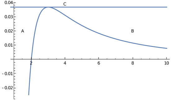  Figure 1. $\tilde{V}$ as function of x. The horizontal line corresponds to the value of $\tilde{V}=1/27$.
• Solutions with $\omega >\frac{1}{27M^2}$, in which case, $R_{\mathsf{\Sigma }}$ is in the interval $[0,\infty ]$ (region C in Figure 1).
• Solutions with $\omega =\frac{1}{27M^2}$, in which case, $R_{\mathsf{\Sigma }}$ may be in the interval $[0,3M]$ or in the interval $[3M,\infty ]$.
• Solutions with $\omega =0$, in which case, $R_{\mathsf{\Sigma }}$ oscillates in the interval $[0,2M]$.

In general, we may write from (65)

$$\alpha (t-t_0)=\pm \int \frac{d{R}_{\mathsf{\Sigma }}}{R_{\mathsf{\Sigma }}^2\sqrt{\omega -V\left(R_{\mathsf{\Sigma }}\right)}},$$

(68)

from which, we may obtain $R_{\mathsf{\Sigma }}$ expressed in terms of elliptic functions. However, in some cases. analytical solutions may be found in terms of elementary functions. For carrying that out, we shall proceed as follows.

Introducing the variable $r=x+b$ in the polynomial

$$P\left(r\right)=a_0{r}^4+a_1{r}^3+a_2{r}^2+a_{3}r+a_4,$$

(69)

we may write

$$\begin{array}{ccc}\hfill P\left(x\right)& =& a_0{x}^4+(a_1+4a_{0}b)x^3+(a_2+3a_{1}b+6a_0{b}^2)x^2+(a_3+2a_{2}b+3a_1{b}^2+4a_0{b}^3)x\hfill \\ & +& a_4+a_{3}b+a_2{b}^2+a_1{b}^3+a_0{b}^4,\hfill \end{array}$$

(70)

or

$$P\left(x\right)={(\sqrt{a_0}x+b_1)}^2(x+b_2)(x+b_3),$$

(71)

where $b_{1,2,3}$ and b are solutions of the following equations:

$$a_4+a_{3}b+a_2{b}^2+a_1{b}^3+a_0{b}^4=b_1^2{b}_2{b}_3,$$

(72)

$$a_3+2a_{2}b+3a_1{b}^2+4a_0{b}^3=b_1^2(b_2+b_3)+2\sqrt{a_0}{b}_1{b}_2{b}_3,$$

(73)

$$a_2+3a_{1}b+6a_0{b}^2=b_1^2+2\sqrt{a_0}{b}_1(b_2+b_3)+a_0{b}_2{b}_3,$$

(74)

$$a_1+4a_{0}b=2\sqrt{a_0}{b}_1+a_0(b_2+b_3).$$

(75)

Then, the integration of (68) produces

$$\pm \int \frac{dx}{(\sqrt{a_0}x+b_1)\sqrt{(x+b_2)(x+b_3)}}=\left\{\genfrac{}{}{0pt}{}{{\beta }_{1}arctan\left({\beta }_2\sqrt{\frac{b_2+x}{b_3+x}}\right)}{{\beta }_1{arctan}^{-1}\left({\beta }_2\sqrt{\frac{b_2+x}{b_3+x}}\right),}\right.$$

(76)

where

$$\begin{array}{ccc}\hfill {\beta }_1& =& \frac{2}{\sqrt{(b_1-\sqrt{a_0}{b}_2)(\sqrt{a_0}{b}_3-b_1)}},\hfill \end{array}$$

(77)

$$\begin{array}{ccc}\hfill {\beta }_2& =& \sqrt{\frac{\sqrt{a_0}{b}_3-b_1}{b_1-\sqrt{a_0}{b}_2}}.\hfill \end{array}$$

(78)

To obtain explicit solutions expressed through elementary functions, we shall assume $b=0$; thus, in our notation, we have

$$\begin{array}{ccc}\hfill a_0& =& \omega ,\hfill \end{array}$$

(79)

$$\begin{array}{ccc}\hfill a_1& =& a_4=0,\hfill \end{array}$$

(80)

$$\begin{array}{ccc}\hfill a_2& =& -1,a_3=2M.\hfill \end{array}$$

(81)

Imposing $b=0$, we are led to two sub-cases, $b_2=0$ and $b_3=0$; in both sub-cases, $M=\frac{1}{3\sqrt{3\omega }}$. Using (79)–(81) in (76), we obtain, for both sub-cases, the same solutions, namely

$$R_{\mathsf{\Sigma }}^{\left(I\right)}=\frac{6M{tanh}^2\left[\frac{\alpha }{2}(t-t_0)\right]}{3-{tanh}^2\left[\frac{\alpha }{2}(t-t_0)\right]},$$

(82)

and

$$R_{\mathsf{\Sigma }}^{\left(II\right)}=\frac{6M{coth}^2\left[\frac{\alpha }{2}(t-t_0)\right]}{3-{coth}^2\left[\frac{\alpha }{2}(t-t_0)\right]}.$$

(83)

In the first case, the areal radius of the boundary ($R_{\mathsf{\Sigma }}^{\left(I\right)}$) expands from 0 (the singularity) approaching $3M$ asymptotically as $t\to \infty$, thereby representing a white hole scenario.

In the second case, the areal radius of the boundary ($R_{\mathsf{\Sigma }}^{\left(II\right)}$) contracts from ∞ (for ${coth}^2\left[\frac{\alpha }{2}(t-t_0)\right]=3)$ approaching $3M$ asymptotically as $t\to \infty$.

Thus, we already have one of the arbitrary functions of time describing our metric. In order to further specify our model, we shall impose the quasi-homologous evolution and the vanishing complexity factor condition.

As we can see from (42), in the non-dissipative case, the quasi-homologous condition implies that the fluid is shear-free ($\sigma =0$), implying, in turn,

$$\frac{\dot{B}}{B}=\frac{\dot{R}}{R}\Rightarrow F\left(t\right)=Const.\equiv F_0.$$

(84)

Thus, the metric functions become

$$A=\frac{F_0}{f\left(t\right)+g\left(r\right)},B=\frac{1}{f\left(t\right)+g\left(r\right)},R=\frac{F_0}{\alpha \left[f\left(t\right)+g\left(r\right)\right]}.$$

(85)

Therefore, our models are now specified up to an arbitrary function of r ($g\left(r\right)$). In order to fix this function, we shall further impose the vanishing complexity factor condition.

Then, feeding back (85) into (31), we obtain

$$\frac{A^{″}}{A}-\frac{A^{\prime }}{A}\left(\frac{B^{\prime }}{B}+\frac{R^{\prime }}{R}\right)=0.$$

(86)

Using (85) in (86), it follows at once that

$$g\left(r\right)=c_{1}r+c_2,$$

(87)

with $c_1\equiv \pm \sqrt{\omega }$, and $c_2$ is another integration constant. We shall choose the negative sign in $c_1$ in order to ensure that $R^{\prime }>0$. However, it should be noticed that the regularity conditions necessary to ensure elementary flatness in the vicinity of the axis of symmetry and, in particular, at the center (see [84,85,86]) are not satisfied.

Therefore, after the imposition of the two conditions above (quasi-homologous evolution and vanishing complexity factor), we have all of the metric functions completely specified for any of the above solutions to (65).

Thus, in the case $b=0$, we obtain from (82) that

$$f^{\left(I\right)}\left(t\right)=\frac{F_0\left\{3-{tanh}^2\left[\frac{\alpha }{2}(t-t_0)\right]\right\}}{6\alpha M{tanh}^2\left[\frac{\alpha }{2}(t-t_0)\right]}-c_1{r}_{\mathsf{\Sigma }}-c_2,$$

(88)

from which, the physical variables are easily found to be

$$\begin{array}{lll}8\pi \mu \hfill & =& -3c_1^2+\frac{{\left\{-F_0-6\alpha c_{1}M(r_{\mathsf{\Sigma }}-r)+3F_0{coth}^2\left[\frac{\alpha }{2}(t-t_0)\right]\right\}}^2}{36F_0^2{M}^2}\hfill \end{array}$$

$$\begin{array}{ccc}& +& \frac{3{cosh}^2\left[\frac{\alpha }{2}(t-t_0)\right]}{4M^2{sinh}^6\left[\frac{\alpha }{2}(t-t_0)\right]},\hfill \end{array}$$

(89)

$$\begin{array}{ccc}\hfill 8\pi P_r& =& \frac{2\alpha c_1(r_{\mathsf{\Sigma }}-r)}{3F_{0}M}-\frac{{\alpha }^2{c}_1^2{(r_{\mathsf{\Sigma }}-r)}^2}{F_0^2}-\frac{3c_1\alpha (r_{\mathsf{\Sigma }}-r)}{2F_{0}M{sinh}^4\left[\frac{\alpha }{2}(t-t_0)\right]},\hfill \end{array}$$

(90)

$$\begin{array}{ccc}\hfill 8\pi P_{\perp }& =& 3c_1^2+\frac{\left[F_0-3\alpha c_{1}M(r_{\mathsf{\Sigma }}-r)\right]}{3F_0{M}^2{sinh}^2\left[\frac{\alpha }{2}(t-t_0)\right]}+\frac{\left[F_0-6\alpha c_{1}M(r_{\mathsf{\Sigma }}-r)\right]}{4F_0{M}^2{sinh}^4\left[\frac{\alpha }{2}(t-t_0)\right]}.\hfill \end{array}$$

(91)

From (89), it follows at once that ${\left(P_r\right)}_{\mathsf{\Sigma }}=0$.

It is worth noting that the expansion scalar for this model reads

$$\mathsf{\Theta }=\frac{3cosh\left[\frac{\alpha }{2}(t-t_0)\right]}{2M{sinh}^3\left[\frac{\alpha }{2}(t-t_0)\right]}.$$

(92)

Thus, the expansion is homogeneous and positive, diverging at $t=t_0$ and tending to zero as $t\to \infty$. The fast braking of the expansion for $t>t_0$ is produced by the negative initially large (diverging at $t=t_0$) value of $D_{T}U$. This can be checked from (A12), where the negative gravitational term proportional to $m/R^2$ provides the leading term in the equation ($\frac{m}{R^2}\sim \frac{1}{{sinh}^4\left[\frac{\alpha }{2}(t-t_0)\right]})$. As time goes on, there is a sharp decrease in the inertial mass density ($\mu +P_r$) as observed from Figure 2, which as $t\to \infty$ becomes arbitrarily small (see (97) below). Now, the striking fact is that the equilibrium is reached asymptotically but not, as usual, by the balance between the gravitational term (the first term on the right of (A12)) and the hydrodynamic terms (the second term on the right of (A12)). Instead, both terms cancel independently. Indeed, as $t\to \infty$, the gravitational term vanishes due to the fact that the inertial mass density (the “passive gravitational mass density”) $\mu +P_r\to 0$, and the hydrodynamic term vanishes because, as can be easily checked, the radial pressure gradient cancels the anisotropic factor, as $t\to \infty$.

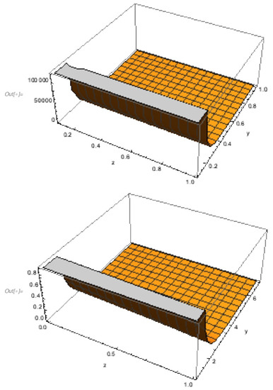
Figure 2. $\tilde{\mu }+{\tilde{P}}_r\equiv 72\pi M^2(\mu +P_r)$ as function of $y\equiv \frac{\alpha }{2}(t-t_0)$ and $z\equiv \frac{r}{r_{\mathsf{\Sigma }}}$ for solution I. In the upper figure, the time interval (y) is $[0.1,1]$, whereas, in the lower figure, it is $[1,7]$.

Next, if we take (83), for $f\left(t\right)$, we obtain

$$f^{\left(II\right)}\left(t\right)=\frac{F_0\left\{3-{coth}^2\left[\frac{\alpha }{2}(t-t_0)\right]\right\}}{6\alpha M{coth}^2\left[\frac{\alpha }{2}(t-t_0)\right]}-c_1{r}_{\mathsf{\Sigma }}-c_2,$$

(93)

whereas the expressions for the physical variables read

$$\begin{array}{rrr}\hfill 8\pi \mu & =& -3c_1^2+\frac{3{sinh}^2\left[\frac{\alpha }{2}(t-t_0)\right]}{4M^2{cosh}^6[\left(\frac{\alpha }{2}(t-t_0)\right]}\hfill \end{array}$$

$$\begin{array}{ccc}& +& \frac{{\left\{F_0+6\alpha c_{1}M(r_{\mathsf{\Sigma }}-r)-3F_0{tanh}^2\left[\frac{\alpha }{2}(t-t_0)\right]\right\}}^2}{36F_0^2{M}^2},\hfill \end{array}$$

(94)

$$\begin{array}{ccc}\hfill 8\pi P_r& =& \frac{2\alpha c_1(r_{\mathsf{\Sigma }}-r)}{3F_{0}M}-\frac{{\alpha }^2{c}_1^2{(r_{\mathsf{\Sigma }}-r)}^2}{F_0^2}-\frac{3c_1\alpha (r_{\mathsf{\Sigma }}-r)}{2F_{0}M{cosh}^4\left[\frac{\alpha }{2}(t-t_0)\right]},\hfill \end{array}$$

(95)

$$\begin{array}{ccc}\hfill 8\pi P_{\perp }& =& 3c_1^2-\frac{F_0-3\alpha c_{1}M(r_{\mathsf{\Sigma }}-r)}{3F_0{M}^2{cosh}^2\left[\frac{\alpha }{2}(t-t_0)\right]}+\frac{F_0-6\alpha c_{1}M(r_{\mathsf{\Sigma }}-r)}{4F_0{M}^2{cosh}^4\left[\frac{\alpha }{2}(t-t_0)\right]}.\hfill \end{array}$$

(96)

In the limit $t\to \infty$, the two above solutions converge to the same static distribution, whose physical variables are

$$\begin{array}{c}\hfill 8\pi \mu =\frac{1}{9M^2}\left[3+{\left(\frac{r}{r_{\mathsf{\Sigma }}}\right)}^2-4\left(\frac{r}{r_{\mathsf{\Sigma }}}\right)\right],\\ \hfill 8\pi P_r=\frac{1}{9M^2}\left[-3-{\left(\frac{r}{r_{\mathsf{\Sigma }}}\right)}^2+4\left(\frac{r}{r_{\mathsf{\Sigma }}}\right)\right],\\ \hfill 8\pi P_{\perp }=\frac{1}{9M^2},\end{array}$$

(97)

where the constant $F_0$ has been chosen $F_0=\frac{r_{\mathsf{\Sigma }}\alpha }{\sqrt{3}}$. It is worth noting that the ensuing equation of state for the static limit is the Chaplygin-type equation $\mu =-P_r$.

In the case where $\omega =0$, the expression for $R_{\mathsf{\Sigma }}$ is given by

$$R_{\mathsf{\Sigma }}^{\left(III\right)}=2M{cos}^2\frac{\alpha }{2}(t-t_0),$$

(98)

and, from (87),

$$\omega =g^{\prime }{\left(r_{\mathsf{\Sigma }}\right)}^2=c_1^2=0.$$

(99)

Then, the following expressions may be obtained for the metric functions

$$A=\frac{F_0}{f\left(t\right)+c_2},B=\frac{1}{f\left(t\right)+c_2},R=\frac{F_0}{\alpha \left[f\left(t\right)+c_2\right]},$$

(100)

the function $f\left(t\right)$

$$f^{III}\left(t\right)=\frac{F_0}{2\alpha M{cos}^2\left[\frac{\alpha }{2}(t-t_0)\right]}-c_2,$$

(101)

and the physical variables

$$\begin{array}{ccc}\hfill 8\pi \mu & =& \frac{\left\{3-2{cos}^2\left[\frac{\alpha }{2}(t-t_0)\right]\right\}}{4M^2{cos}^6\left[\frac{\alpha }{2}(t-t_0)\right]},\hfill \end{array}$$

(102)

$$\begin{array}{ccc}\hfill 8\pi P_r& =& 0,\hfill \end{array}$$

(103)

$$\begin{array}{ccc}\hfill 8\pi P_{\perp }& =& \frac{1}{4M^2{cos}^4\left[\frac{\alpha }{2}(t-t_0)\right]}.\hfill \end{array}$$

(104)

It is worth stressing the presence of topological pathologies of this solution (e.g., $R^{\prime }=0$), implying the appearance of the shell crossing singularities.

Before closing this subsection, we would like to call attention to a very peculiar solution that may be obtained by assuming that the space–time outside the boundary surface delimiting the fluid is Minkowski. This implies $M=0$, and then the solutions to (63) read

$$R_{\mathsf{\Sigma }}^{\left(IV\right)}=\frac{1}{\sqrt{\omega }cos\left[\alpha (t-t_0)\right]},$$

(105)

and

$$R_{\mathsf{\Sigma }}^{\left(V\right)}=\frac{1}{\sqrt{\omega }sin\left[\alpha (t-t_0)\right]}.$$

(106)

Then, assuming further that the evolution is quasi-homologous and the complexity factor vanishes, for the functions $f\left(t\right)$, we obtain

$$f^{\left(IV\right)}\left(t\right)=\frac{1}{\alpha }{F}_0\sqrt{\omega }cos\left[\alpha (t-t_0)\right]+\sqrt{\omega }{r}_{\mathsf{\Sigma }}-c_2,$$

(107)

and

$$f^{\left(V\right)}\left(t\right)=\frac{1}{\alpha }{F}_0\sqrt{\omega }sin\left[\alpha (t-t_0)\right]+\sqrt{\omega }{r}_{\mathsf{\Sigma }}-c_2.$$

(108)

The corresponding physical variables for $f^{\left(IV\right)}$ read

$$\begin{array}{ccc}\hfill 8\pi \mu & =& -2\omega {cos}^2\left[\alpha (t-t_0)\right]\hfill \\ & +& \omega (1-\frac{r}{r_{\mathsf{\Sigma }}})\left[1-\frac{r}{r_{\mathsf{\Sigma }}}+2cos\left[\alpha (t-t_0)\right]\right],\hfill \end{array}$$

(109)

$$8\pi P_r=-\omega \left(1-\frac{r}{r_{\mathsf{\Sigma }}}\right)\left[4cos\left[\alpha (t-t_0)\right]+1-\frac{r}{r_{\mathsf{\Sigma }}}\right],$$

(110)

$$8\pi P_{\perp }=\omega {cos}^2\left[\alpha (t-t_0)\right]-2\omega \left(1-\frac{r}{r_{\mathsf{\Sigma }}}\right)cos\left[\alpha (t-t_0)\right],$$

(111)

whereas, for $f^{\left(V\right)}$, they are

$$\begin{array}{ccc}\hfill 8\pi \mu & =& -2\omega {sin}^2\left[\alpha (t-t_0)\right]\hfill \\ & +& \omega (1-\frac{r}{r_{\mathsf{\Sigma }}})\left[1-\frac{r}{r_{\mathsf{\Sigma }}}+2sin\left[\alpha (t-t_0)\right]\right],\hfill \end{array}$$

(112)

$$8\pi P_r=-\omega \left(1-\frac{r}{r_{\mathsf{\Sigma }}}\right)\left[4sin\left[\alpha (t-t_0)\right]+1-\frac{r}{r_{\mathsf{\Sigma }}}\right],$$

(113)

$$8\pi P_{\perp }=\omega {sin}^2\left[\alpha (t-t_0)\right]-2\omega \left(1-\frac{r}{r_{\mathsf{\Sigma }}}\right)sin\left[\alpha (t-t_0)\right].$$

(114)

In the above, the constants $F_0,\alpha ,r_{\mathsf{\Sigma }}$ have been chosen such that $\frac{F_0}{\alpha r_{\mathsf{\Sigma }}}=1$.

These kinds of configurations have been considered in [11,87].

5.2. ${\chi }_{\alpha }{V}^{\alpha }=0;q\ne 0$

Let us now consider the general dissipative case.

Then, from (49), following the same procedure as in the non-dissipative case, we obtain

$$A=\alpha R,$$

(115)

where $\alpha$ is a unit constant with dimensions of $\frac{1}{length}$,

$$F\left(t\right)B=\alpha R,$$

(116)

where $F\left(t\right)$ is and arbitrary function of t, and

$${\chi }_{,1}^1=0\Rightarrow {\chi }^1=constant.$$

(117)

Then, feeding back (115) and (116) into (A3) with $q\ne 0$, one obtains

$$\frac{{\dot{B}}^{\prime }}{B}-\frac{2\dot{B}{B}^{\prime }}{B^2}=4\pi qAB.$$

(118)

The equation above may be formally integrated to obtain

$$B=\frac{1}{f\left(t\right)+g\left(r\right)-4\pi \int \int qAdtdr},$$

(119)

$$A=\alpha R=\frac{F\left(t\right)}{f\left(t\right)+g\left(r\right)-4\pi \int \int qAdtdr},$$

(120)

where f and g are two arbitrary functions of their arguments.

In order to find a specific solution, we shall next impose the vanishing complexity factor condition ($Y_{TF}=0$).

Then, from the above expressions and (31), the condition $Y_{TF}=0$ reads

$$\frac{1}{F^2}\left(\frac{\ddot{F}}{F}+\frac{\dot{F}\dot{B}}{FB}-\frac{{\dot{F}}^2}{F^2}\right)+\frac{B^{″}}{B}-2{\left(\frac{B^{\prime }}{B}\right)}^2=0.$$

(121)

In order to find a solution to the above equation, we shall assume that

$$\left(\frac{\ddot{F}}{F}+\frac{\dot{F}\dot{B}}{FB}-\frac{{\dot{F}}^2}{F^2}\right)=0,$$

(122)

and

$$\frac{B^{″}}{B}-2{\left(\frac{B^{\prime }}{B}\right)}^2=0.$$

(123)

The integration of (123) produces

$$B=-\frac{1}{\beta \left(t\right)r+\gamma \left(t\right)},$$

(124)

where $\beta ,\gamma$ are arbitrary functions of t. It is worth noting that $\beta$ has dimensions of $\frac{1}{length}$, and that $\gamma$ is dimensionless.

Next, taking the r derivative of (122), we obtain $\gamma =\frac{\beta }{\alpha }$.

Then, we may write

$$B=-\frac{\alpha }{\beta \left(t\right)(\alpha r+1)}.$$

(125)

Next, combining (122) with (125), we obtain

$$F\left(t\right)=c_3{e}^{c_4\int \beta dt},$$

(126)

where $c_3,c_4$ are arbitrary constants.

From the above expression, it follows at once that

$$\frac{\dot{F}}{F}=c_4\beta .$$

(127)

On the other hand, (119) with (125) imply that

$$4\pi \int \int qAdtdr=\beta \left(t\right)r,g\left(r\right)=g_{1}r+g_0,$$

(128)

where $g_1,g_0$ are constant.

We may now write the physical variables in terms of the function $\beta \left(t\right)$; they read

$$8\pi \mu =\frac{{\beta }^2{(\alpha r+1)}^2}{{\alpha }^2{c}_3^2{e}^{2c_4\int \beta dt}}\left({\alpha }^2-4c_4\dot{\beta }+\frac{3{\dot{\beta }}^2}{{\beta }^2}+c_4^2{\beta }^2\right)-3{\beta }^2,$$

(129)

$$4\pi q=-\frac{\beta \dot{\beta }(\alpha r+1)}{\alpha c_3{e}^{c_4\int \beta dt}},$$

(130)

$$8\pi P_r=-\frac{{\beta }^2{(\alpha r+1)}^2}{{\alpha }^2{c}_3^2{e}^{2c_4\int \beta dt}}\left({\alpha }^2-\frac{2\ddot{\beta }}{\beta }+\frac{3{\dot{\beta }}^2}{{\beta }^2}+c_4^2{\beta }^2\right)+3{\beta }^2,$$

(131)

$$8\pi P_{\perp }=-\frac{{\beta }^2{(\alpha r+1)}^2}{{\alpha }^2{c}_3^2{e}^{2c_4\int \beta dt}}\left(c_4\dot{\beta }-\frac{2\ddot{\beta }}{\beta }+\frac{3{\dot{\beta }}^2}{{\beta }^2}\right)+3{\beta }^2.$$

(132)

The function $\beta$ may be found, in principle, from the junction condition (35); however, this is in practice quite difficult. Therefore, we shall next explore the way to impose further constraints on our fluid distribution in order to simplify the models, and, afterwards, we shall use the junction conditions.

We shall start by imposing the quasi-homologous condition (46). Then, using (119) and (120) in (46), we obtain

$$4\pi qA\frac{B^2}{B^{\prime }}=\frac{\dot{F}}{F}.$$

(133)

Using (133) with (125)–(128), one obtains

$$\beta =-\frac{1}{c_{4}t+c_5},$$

(134)

where $c_5$ is a constant with dimensions of $length$.

Thus, the metric functions may be written as

$$B=\frac{\alpha (c_{4}t+c_5)}{(\alpha r+1)},$$

(135)

$$A=\alpha R=\frac{c_3}{\alpha r+1}.$$

(136)

It is worth noting that the areal radius is independent of time ($U=0$); solutions of this kind have been found in [69].

Next, instead of the quasi-homologous condition, we shall impose the shear-free condition. Then, assuming that $\sigma =0$, it follows at once that $\dot{F}=0$ implying $c_4=0$. Then, the metric functions become

$$B=-\frac{\alpha }{\beta (\alpha r+1)},A=-\frac{c_3\alpha }{\beta (\alpha r+1)},R=-\frac{c_3}{\beta (\alpha r+1)},$$

(137)

from which, we can write the physical variables as

$$8\pi \mu =\frac{{\beta }^2{(\alpha r+1)}^2}{{\alpha }^2{c}_3^2}\left({\alpha }^2+\frac{3{\dot{\beta }}^2}{{\beta }^2}\right)-3{\beta }^2,$$

(138)

$$4\pi q=-\frac{\beta \dot{\beta }(\alpha r+1)}{\alpha c_3},$$

(139)

$$8\pi P_r=-\frac{{\beta }^2{(\alpha r+1)}^2}{{\alpha }^2{c}_3^2}\left({\alpha }^2-\frac{2\ddot{\beta }}{\beta }+\frac{3{\dot{\beta }}^2}{{\beta }^2}\right)+3{\beta }^2,$$

(140)

$$8\pi P_{\perp }=-\frac{{\beta }^2{(\alpha r+1)}^2}{{\alpha }^2{c}_3^2}\left(-\frac{2\ddot{\beta }}{\beta }+\frac{3{\dot{\beta }}^2}{{\beta }^2}\right)+3{\beta }^2.$$

(141)

We can find $\beta$ from the junction condition (35), which, using (139) and (140), reads

$$\frac{2\ddot{\beta }}{\beta }-3{\left(\frac{\dot{\beta }}{\beta }\right)}^2+\frac{2{\alpha }_1\dot{\beta }}{\beta }={\alpha }^2-3{\alpha }_1^2,$$

(142)

with

$${\alpha }_1\equiv \frac{\alpha c_3}{\alpha r_{\mathsf{\Sigma }}+1}.$$

(143)

In order to integrate the above equation, let us introduce the variable $s=\frac{\dot{\beta }}{\beta }$, which casts (142) into the Ricatti equation

$$2\dot{s}-s^2+2{\alpha }_{1}s={\alpha }^2-3{\alpha }_1^2,$$

(144)

whose solution is

$$s={\alpha }_1+\sqrt{{\alpha }^2-4{\alpha }_1^2}tan\left[\frac{\sqrt{{\alpha }^2-4{\alpha }_1^2}}{2}(t-t_0)\right],$$

(145)

producing, for $\beta$,

$$\beta \left(t\right)={\alpha }_2{e}^{{\alpha }_{1}t}{sec}^2\left[\frac{\sqrt{{\alpha }^2-4{\alpha }_1^2}}{2}(t-t_0)\right],$$

(146)

where ${\alpha }_2$ is a negative constant of integration with the same dimensions as $\beta$.

Using the truncated version of the transport equation (39), for the temperature, we obtain

$$T(t,r)=\frac{\alpha r+1}{4\pi c_3\kappa \alpha }\left[\frac{\tau r({\dot{\beta }}^2+\beta \ddot{\beta })}{c_3}-\dot{\beta }ln(\alpha r+1)\right]+T_0\left(t\right),$$

(147)

where $c_3$ and $T_0\left(t\right)$ are an arbitrary constant and function of integration, respectively. The model described by Equations (137)–(141) and (146), (147) will be named as model $VI$.

5.3. $q=0;{\chi }^{\alpha }\left|\right|V^{\alpha }$

We shall next analyze the case when the CKV is parallel to the four-velocity vector. We start by considering the non-dissipative case. In this case, Equation (49) produces

$$A=Bh\left(r\right),R=Br,{\chi }^0=1,\psi =\frac{\dot{B}}{B},$$

(148)

where $h\left(r\right)$ is an arbitrary function of its argument and ${\chi }^1=0$. It is worth noting that, in this case, the fluid is necessarily shear-free.

Thus, the line element may be written as

$$d{s}^2=B^2\left[-h^2\left(r\right)d{t}^2+d{r}^2+r^2(d{\theta }^2+{sin}^2\theta d{\varphi }^2)\right].$$

(149)

Next, using (148) in (A3), the condition $q=0$ reads

$$\frac{{\dot{R}}^{\prime }}{R}-2\frac{\dot{R}}{R}\frac{R^{\prime }}{R}-\frac{\dot{R}}{R}\left(\frac{h^{\prime }}{h}-\frac{1}{r}\right)=0,$$

(150)

whose solution is

$$\begin{array}{c}\hfill R=\frac{r}{h\left(r\right)\left[f\left(t\right)+g\left(r\right)\right]},\end{array}$$

(151)

implying that

$$\begin{array}{c}\hfill B=\frac{1}{h\left(r\right)\left[f\left(t\right)+g\left(r\right)\right]},A=\frac{1}{f\left(t\right)+g\left(r\right)},\end{array}$$

(152)

where $g,f$ are two arbitrary functions of their argument.

Thus, the metric is defined up to three arbitrary functions ($g\left(r\right),f\left(t\right),h\left(r\right)$).

The function $f\left(t\right)$ will be obtained from the junction conditions (33) and (35).

Indeed, evaluating the mass function at the boundary surface $\mathsf{\Sigma }$, from (33) and (151), we obtain

$${\dot{R}}_{\mathsf{\Sigma }}^2={\alpha }^2{R}_{\mathsf{\Sigma }}^4\left[ϵ-V\left(R_{\mathsf{\Sigma }}\right)\right],$$

(153)

where ${\alpha }^2\equiv \frac{h_{\mathsf{\Sigma }}^2}{r_{\mathsf{\Sigma }}^2}$, $ϵ\equiv {\left(g^{\prime }\right)}_{\mathsf{\Sigma }}^2{h}_{\mathsf{\Sigma }}^2$, and

$$V\left(R_{\mathsf{\Sigma }}\right)=\frac{2\sqrt{ϵ}}{R_{\mathsf{\Sigma }}}(1-a_1)+\frac{a_1}{R_{\mathsf{\Sigma }}^2}(2-a_1)-\frac{2M}{R_{\mathsf{\Sigma }}^3},$$

(154)

with $a_1\equiv \frac{h_{\mathsf{\Sigma }}^{\prime }{r}_{\mathsf{\Sigma }}}{h_{\mathsf{\Sigma }}}$.

On the other hand, from (35), using (151), we obtain

$$\begin{array}{c}\hfill 2{\ddot{R}}_{\mathsf{\Sigma }}{R}_{\mathsf{\Sigma }}-{\dot{R}}_{\mathsf{\Sigma }}^2-3ϵ{\alpha }^2{R}_{\mathsf{\Sigma }}^4-4{\alpha }^2\sqrt{ϵ}{R}_{\mathsf{\Sigma }}^3(a_1-1)-{\alpha }^2{R}_{\mathsf{\Sigma }}^2{a}_1(a_1-2)=0.\end{array}$$

(155)

To specify a model, we have to obtain $f\left(t\right)$ from the solution to the above equations.

In the special case $a_1=1$, (153) becomes

$${\dot{R}}_{\mathsf{\Sigma }}^2={\alpha }^2{R}_{\mathsf{\Sigma }}^4\left[ϵ-\frac{1}{R_{\mathsf{\Sigma }}^2}+\frac{2M}{R_{\mathsf{\Sigma }}^3}\right],$$

(156)

which has exactly the same form as (65) and therefore admits the same kind of solutions, and (155) reads

$$\begin{array}{c}\hfill 2{\ddot{R}}_{\mathsf{\Sigma }}{R}_{\mathsf{\Sigma }}-{\dot{R}}_{\mathsf{\Sigma }}^2-3ϵ{\alpha }^2{R}_{\mathsf{\Sigma }}^4+{\alpha }^2{R}_{\mathsf{\Sigma }}^2=0,\end{array}$$

(157)

a first integral of which, as can be easily shown, is (156); therefore, we only need to satisfy (156).

In order to determine the functions $g\left(r\right),h\left(r\right)$, we shall assume the vanishing complexity factor condition $Y_{TF}=0$.

Using (151) in (31), the condition $Y_{TF}=0$ reads

$$\frac{g^{″}}{g^{\prime }}-\frac{1}{r}+\frac{2h^{\prime }}{h}=0,$$

(158)

or

$$\frac{v^{\prime }}{v}-\frac{1}{r}+\frac{2h^{\prime }}{h}=0,$$

(159)

with $v\equiv g^{\prime }$, whose formal solution is

$$v=\frac{c_{4}r}{h^2},$$

(160)

producing

$$g=c_4\int \frac{r}{h^2}dr+c_5,$$

(161)

where $c_4,c_5$ are arbitrary constants.

If we choose

$$h\left(r\right)=c_{6}r,$$

(162)

implying $a_1=1$, then, from (161), we obtain

$$g=c_{7}lnr+c_5,$$

(163)

where $c_6,c_7$ are constants.

Thus, let us consider the following model. The time dependence described by $f\left(t\right)$ is obtained from the solution to (156) given by

$$R_{\mathsf{\Sigma }}^{\left(VII\right)}=\frac{6M{tanh}^2\left[\frac{\alpha }{2}(t-t_0)\right]}{3-{tanh}^2\left[\frac{\alpha }{2}(t-t_0)\right]},$$

(164)

with $ϵ=\frac{1}{27M^2}$, and the radial dependence of the model is given by the functions $g\left(r\right),h\left(r\right)$ given by (162) and (163).

The physical variables corresponding to this model read

$$\begin{array}{ccc}\hfill & & 8\pi \mu =\frac{3{coth}^2\left[\frac{\alpha }{2}(t-t_0)\right]}{4M^2{sinh}^4\left[\frac{\alpha }{2}(t-t_0)\right]}+\frac{{(3{coth}^2\left[\frac{\alpha }{2}(t-t_0)\right]-1)}^2}{36M^2}\hfill \\ & -& \frac{1}{9M^2}+ln\left(\frac{r}{r_{\mathsf{\Sigma }}}\right)\left[\frac{3{coth}^2\left[\frac{\alpha }{2}(t-t_0)\right]-1}{9\sqrt{3}{M}^2}+\frac{1}{27M^2}ln\left(\frac{r}{r_{\mathsf{\Sigma }}}\right)\right],\hfill \end{array}$$

(165)

$$\begin{array}{c}\hfill 8\pi P_r=ln\left(\frac{r}{r_{\mathsf{\Sigma }}}\right)\left[\frac{(3{coth}^2\left[\frac{\alpha }{2}(t-t_0)\right]-1)(3{coth}^2\left[\frac{\alpha }{2}(t-t_0)\right]-5)}{18\sqrt{3}{M}^2}-\frac{1}{27M^2}ln\left(\frac{r}{r_{\mathsf{\Sigma }}}\right)\right],\end{array}$$

(166)

$$\begin{array}{c}\hfill 8\pi P_{\perp }=\frac{(3{coth}^2\left[\frac{\alpha }{2}(t-t_0)\right]+1)}{12M^2{sinh}^2\left[\frac{\alpha }{2}(t-t_0)\right]}+\frac{1}{9M^2}+ln\left(\frac{r}{r_{\mathsf{\Sigma }}}\right)\frac{(3{coth}^2\left[\frac{\alpha }{2}(t-t_0)\right]-1)}{6\sqrt{3}{M}^2{sinh}^2[\frac{\alpha }{2}(t-t_0)},\end{array}$$

(167)

where the following relationships between the constants have been used: ${\alpha }^2\equiv c_6^2$, $ϵ\equiv \frac{1}{27M^2}\equiv c_7^2{c}_6^2$.

In the limit $t\to \infty$, the above model tends to a static fluid distribution described by

$$\begin{array}{c}\hfill 8\pi \mu =ln\left(\frac{r}{r_{\mathsf{\Sigma }}}\right)\left[\frac{2}{9\sqrt{3}{M}^2}+\frac{1}{27M^2}ln\left(\frac{r}{r_{\mathsf{\Sigma }}}\right)\right],\end{array}$$

(168)

$$8\pi P_r=-ln\left(\frac{r}{r_{\mathsf{\Sigma }}}\right)\left[\frac{2}{9\sqrt{3}{M}^2}+\frac{1}{27M^2}ln\left(\frac{r}{r_{\mathsf{\Sigma }}}\right)\right],$$

(169)

$$\begin{array}{c}\hfill 8\pi P_{\perp }=\frac{1}{9M^2},\end{array}$$

(170)

satisfying the equation of state $P_r=-\mu$.

Another case that allows for integration in terms of the elementary function may be obtained from the conditions $ϵ=0$ and $a_1=1/2$. Then, (153) reads

$${\dot{R}}_{\mathsf{\Sigma }}^2={\alpha }^2{R}_{\mathsf{\Sigma }}^4\left[\frac{2M}{R_{\mathsf{\Sigma }}^3}-\frac{3}{4R_{\mathsf{\Sigma }}^2}\right].$$

(171)

The above equation may be easily integrated, producing

$$R_{\mathsf{\Sigma }}^{\left(VIII\right)}=\frac{4M}{3}\left(1+sin\tilde{t}\right),$$

(172)

with $\tilde{t}\equiv \frac{\sqrt{3}\alpha }{2}(t-t_0)$.

Next, in order to further specify the model, we shall impose the vanishing complexity factor condition. In this case ($a_1=1/2$), the general solution to (159) reads

$$h=c_1\sqrt{r},g=c_{2}r+c_3,$$

(173)

However, since $ϵ=0$, the constant $c_2$ must vanish.

The physical variables for this model read

$$\begin{array}{c}\hfill 8\pi \mu =\frac{27}{64M^2{(1+sin\tilde{t})}^2}\left[\frac{3{cos}^2\tilde{t}}{{(1+sin\tilde{t})}^2}+\frac{r_{\mathsf{\Sigma }}}{r}\right],\end{array}$$

(174)

$$\begin{array}{c}\hfill 8\pi P_r=\frac{27}{64M^2{(1+sin\tilde{t})}^2}\left(1-\frac{r_{\mathsf{\Sigma }}}{r}\right),\end{array}$$

(175)

$$\begin{array}{c}\hfill 8\pi P_{\perp }=\frac{27}{64M^2{(1+sin\tilde{t})}^2}.\end{array}$$

(176)

This solution represents the fluid distribution oscillating between $R_{\mathsf{\Sigma }}=0$ and $R_{\mathsf{\Sigma }}=\frac{8M}{3}$. It is worth noting that the energy density is always positive, whereas the radial pressure is not.

Finally, we shall present two solutions describing a “ghost” compact object of the kind already discussed in the previous section.

Thus, assuming $M=0$, Equation (153) becomes

$${\dot{R}}_{\mathsf{\Sigma }}^2={\alpha }^2{R}_{\mathsf{\Sigma }}^4\left[ϵ-\frac{2\sqrt{ϵ}(1-a_1)}{R_{\mathsf{\Sigma }}}-\frac{a_1(2-a_1)}{R_{\mathsf{\Sigma }}^2}\right].$$

(177)

Solutions to the above equation in terms of elementary functions may be obtained by assuming $a_1=1$, in which case, the two possible solutions to (177) are

$$R_{\mathsf{\Sigma }}^{\left(IX\right)}=\frac{1}{\sqrt{ϵ}cos\left[\alpha (t-t_0)\right]},$$

(178)

and

$$R_{\mathsf{\Sigma }}^{\left(X\right)}=\frac{1}{\sqrt{ϵ}sin\left[\alpha (t-t_0)\right]}.$$

(179)

Further imposing the vanishing complexity factor condition, functions $h\left(r\right),g\left(r\right)$ are given by (162) and (163). The physical variables corresponding to (178) and (179) read, respectively,

$$8\pi \mu =-2ϵ{cos}^2\left[\alpha (t-t_0)\right]+ϵln\frac{r}{r_{\mathsf{\Sigma }}}\left[2cos\left[\alpha (t-t_0)\right]+ln\frac{r}{r_{\mathsf{\Sigma }}}\right],$$

(180)

$$8\pi P_r=-ϵln\frac{r}{r_{\mathsf{\Sigma }}}\left[4cos\left[\alpha (t-t_0)\right]+ln\frac{r}{r_{\mathsf{\Sigma }}}\right],$$

(181)

$$8\pi P_{\perp }=ϵ{cos}^2\left[\alpha (t-t_0)\right]-2ϵln\frac{r}{r_{\mathsf{\Sigma }}}cos\left[\alpha (t-t_0)\right],$$

(182)

and

$$8\pi \mu =-2ϵ{sin}^2\left[\alpha (t-t_0)\right]+ϵln\frac{r}{r_{\mathsf{\Sigma }}}\left[2sin\left[\alpha (t-t_0)\right]+ln\frac{r}{r_{\mathsf{\Sigma }}}\right],$$

(183)

$$\begin{array}{c}\hfill 8\pi P_r=-ϵln\frac{r}{r_{\mathsf{\Sigma }}}\left[4sin\left[\alpha (t-t_0)\right]+ln\frac{r}{r_{\mathsf{\Sigma }}}\right],\end{array}$$

(184)

$$8\pi P_{\perp }=ϵ{sin}^2\left[\alpha (t-t_0)\right]-2ϵln\frac{r}{r_{\mathsf{\Sigma }}}sin\left[\alpha (t-t_0)\right].$$

(185)

5.4. ${\chi }^{\alpha }\left|\right|V^{\alpha };q\ne 0$

Finally, we shall consider the case where the CKV is parallel to the four-velocity and the system is dissipative. As result of the admittance of the CKV, the metric functions read as (148). Then, feeding this back into (A3) produces

$$\frac{{\dot{B}}^{\prime }}{B}-2\frac{\dot{B}}{B}\frac{B^{\prime }}{B}-\frac{\dot{B}}{B}\frac{h^{\prime }}{h}=4\pi qAB,$$

(186)

which may be formally integrated to obtain

$$B=\frac{1}{h\left(r\right)\left[f\left(t\right)+g\left(r\right)-\int \int 4\pi qBdrdt\right]},$$

(187)

implying that

$$A=\frac{1}{\left[f\left(t\right)+g\left(r\right)-\int \int 4\pi qBdrdt\right]},$$

(188)

and

$$R=\frac{r}{h\left(r\right)\left[f\left(t\right)+g\left(r\right)-\int \int 4\pi qBdrdt\right]},$$

(189)

where $f\left(t\right)$ and $g\left(r\right)$ are arbitrary functions of their arguments.

To specify a model, we shall impose the vanishing complexity factor condition. Thus, using (187)–(189) in (31), the condition $Y_{TF}=0$ reads

$$g^{\prime }-\int 4\pi qBdt=\frac{\gamma \left(t\right)r}{h^2\left(r\right)},$$

(190)

a formal integration of which produces

$$g-\int \int 4\pi qBdtdr=\gamma \left(t\right)\int \frac{rdr}{h^2\left(r\right)},$$

(191)

where $\gamma \left(t\right)$ is an arbitrary function.

In addition, taking the t-derivative of (190), we obtain

$$4\pi qB=-\frac{\dot{\gamma }\left(t\right)r}{h^2\left(r\right)}.$$

(192)

Using the above expressions, we may write the metric functions (187)–(189) as

$$B=\frac{1}{h\left(r\right)\left[f\left(t\right)+\gamma \left(t\right)\int \frac{rdr}{h^2\left(r\right)}\right]},$$

(193)

implying that

$$A=\frac{1}{\left[f\left(t\right)+\gamma \left(t\right)\int \frac{rdr}{h^2\left(r\right)}\right]},$$

(194)

and

$$R=\frac{r}{h\left(r\right)\left[f\left(t\right)+\gamma \left(t\right)\int \frac{rdr}{h^2\left(r\right)}\right]}.$$

(195)

Further restrictions on functions $f\left(t\right),\gamma \left(t\right)$ will be obtained from the junction condition ${(P_r=q)}_{\mathsf{\Sigma }}$.

Indeed, using (192)–(195) and (A4), the condition ${(P_r=q)}_{\mathsf{\Sigma }}$ reads

$$\begin{array}{ccc}& & h_{\mathsf{\Sigma }}^2{X}_{\mathsf{\Sigma }}\left(\frac{1}{r_{\mathsf{\Sigma }}}-\frac{h_{\mathsf{\Sigma }}^{\prime }}{h_{\mathsf{\Sigma }}}-\frac{X_{\mathsf{\Sigma }}^{\prime }}{X_{\mathsf{\Sigma }}}\right)\left(\frac{1}{r_{\mathsf{\Sigma }}}-\frac{h_{\mathsf{\Sigma }}^{\prime }}{h_{\mathsf{\Sigma }}}-3\frac{X_{\mathsf{\Sigma }}^{\prime }}{X_{\mathsf{\Sigma }}}\right)\hfill \\ & -& X_{\mathsf{\Sigma }}\left(-2\frac{{\ddot{X}}_{\mathsf{\Sigma }}}{X_{\mathsf{\Sigma }}}+3\frac{{\dot{X}}_{\mathsf{\Sigma }}^2}{X_{\mathsf{\Sigma }}^2}+{\alpha }^2\right)=-\frac{2\dot{\gamma }}{\alpha },\hfill \end{array}$$

(196)

where

$$X\equiv f\left(t\right)+\gamma \left(t\right)\int \frac{rdr}{h^2\left(r\right)},\alpha \equiv \frac{h_{\mathsf{\Sigma }}}{r_{\mathsf{\Sigma }}}.$$

(197)

In order to solve the above equation, we shall assume that

$$\begin{array}{c}\hfill -2\frac{{\ddot{X}}_{\mathsf{\Sigma }}}{X_{\mathsf{\Sigma }}}+3\frac{{\dot{X}}_{\mathsf{\Sigma }}^2}{X_{\mathsf{\Sigma }}^2}+{\alpha }^2=\frac{2\dot{\gamma }}{X_{\mathsf{\Sigma }}\alpha },\end{array}$$

(198)

and

$$1-a_1-\frac{r_{\mathsf{\Sigma }}{X}_{\mathsf{\Sigma }}^{\prime }}{X_{\mathsf{\Sigma }}}=0,$$

(199)

where $a_1\equiv \frac{h_{\mathsf{\Sigma }}^{\prime }{r}_{\mathsf{\Sigma }}}{h_{\mathsf{\Sigma }}}$.

From (199), it follows at once that

$$1-a_1=\frac{\gamma \left(t\right)}{{\alpha }^2{X}_{\mathsf{\Sigma }}},$$

(200)

producing

$$\frac{\gamma \left(t\right){\dot{X}}_{\mathsf{\Sigma }}}{X_{\mathsf{\Sigma }}^2}=\frac{\dot{\gamma }\left(t\right)}{X_{\mathsf{\Sigma }}}.$$

(201)

Using (200) and (201) in (198), this last equation becomes

$$\begin{array}{c}\hfill 2\frac{{\ddot{X}}_{\mathsf{\Sigma }}}{X_{\mathsf{\Sigma }}}-3\frac{{\dot{X}}_{\mathsf{\Sigma }}^2}{X_{\mathsf{\Sigma }}^2}+\frac{2\alpha {\dot{X}}_{\mathsf{\Sigma }}(1-a_1)}{X_{\mathsf{\Sigma }}}-{\alpha }^2=0.\end{array}$$

(202)

In order to integrate (202), let us introduce the variable $y=\frac{{\dot{X}}_{\mathsf{\Sigma }}}{X_{\mathsf{\Sigma }}}$, in terms of which, (202) reads

$$\dot{y}-\frac{1}{2}{y}^2+\alpha (1-a_1)y-\frac{{\alpha }^2}{2}=0.$$

(203)

This is a Ricatti equation, a particular solution of which is

$$y_0=\alpha (1-a_1)\pm \alpha \sqrt{a_1^2-2a_1}.$$

(204)

Then, in order to find the general solution to (203), let us introduce the variable $z=y-y_0$, producing

$$\dot{z}-\frac{1}{2}{z}^2+\left[\alpha (1-a_1)-y_0\right]z=0,$$

(205)

whose solution reads

$$z=\frac{2\delta }{1+b{e}^{\delta t}},$$

(206)

where b is an arbitrary constant of integration and $\delta \equiv \alpha (1-a_1)-y_0$.

With this result, we can easily find $X_{\mathsf{\Sigma }}$, whose expression reads

$$X_{\mathsf{\Sigma }}=\frac{c{e}^{(2\delta +y_0)t}}{{(1+b{e}^{\delta t})}^2},$$

(207)

where c is a constant of integration.

Using (207) in (200), we obtain the explicit form of $\gamma \left(t\right)$, and, using this expression and (207) in (197), we obtain the explicit form of $f\left(t\right)$. Thus, the model is completely determined up to a single function of r ($h\left(r\right)$).

In terms of $X(t,r)$ and $h\left(r\right)$, the physical variables read

$$\begin{array}{c}\hfill 8\pi \mu =3{\dot{X}}^2-h^2{X}^2\left[-\frac{2h^{″}}{h}+\frac{3{\left(h^{\prime }\right)}^2}{h^2}-\frac{2X^{″}}{X}+\frac{3{\left(X^{\prime }\right)}^2}{X^2}+\frac{2h^{\prime }{X}^{\prime }}{hX}-\frac{4h^{\prime }}{rh}-\frac{4X^{\prime }}{rX}\right],\end{array}$$

(208)

$$\begin{array}{c}\hfill 8\pi P_r=2\ddot{X}X-3{\dot{X}}^2+h^2{X}^2\left[\frac{{\left(h^{\prime }\right)}^2}{h^2}+\frac{3{\left(X^{\prime }\right)}^2}{X^2}+\frac{4h^{\prime }{X}^{\prime }}{hX}-\frac{2h^{\prime }}{rh}-\frac{4X^{\prime }}{rX}\right],\end{array}$$

(209)

$$\begin{array}{c}\hfill 8\pi P_{\perp }=2\ddot{X}X-3{\dot{X}}^2+h^2{X}^2\left[-\frac{h^{″}}{h}+\frac{{\left(h^{\prime }\right)}^2}{h^2}-\frac{2X^{″}}{X}+\frac{3{\left(X^{\prime }\right)}^2}{X^2}-\frac{h^{\prime }}{rh}-\frac{2X^{\prime }}{rX}\right],\end{array}$$

(210)

$$\begin{array}{c}\hfill 8\pi q=-2hX{\dot{X}}^{\prime }.\end{array}$$

(211)

In order to obtain a specific model, we shall assume that $a_1=2$, which implies that $y_0=-\alpha$ and $\delta =0$; then, feeding back these values in (207), the expression for $X_{\mathsf{\Sigma }}$ becomes

$$X_{\mathsf{\Sigma }}=\tilde{c}{e}^{-\alpha t},$$

(212)

with $\tilde{c}\equiv \frac{c}{{(1+b)}^2}$.

Next, we shall assume for $h\left(r\right)$ the form

$$h\left(r\right)=c_2{r}^2,$$

(213)

where $c_2$ is a constant with dimensions $1/{\left[length\right]}^2$, producing

$$\alpha =c_2{r}_{\mathsf{\Sigma }}.$$

(214)

Using (213) and (214), for the radial dependence of X, we obtain

$$\int \frac{rdr}{h{\left(r\right)}^2}=-\frac{r_{\mathsf{\Sigma }}^2}{2{\alpha }^2{r}^2}.$$

(215)

From (200), for $\gamma \left(t\right)$, we obtain at once

$$\gamma \left(t\right)=-{\alpha }^2\tilde{c}{e}^{-\alpha t},$$

(216)

and from (197) and (215), the expression for $f\left(t\right)$ reads

$$f\left(t\right)=\frac{\tilde{c}{e}^{-\alpha t}}{2}.$$

(217)

Finally, the expression for $X(t,r)$ reads

$$X^{\left(XI\right)}(t,r)=\frac{\tilde{c}{e}^{-\alpha t}}{2}\left[1+{\left(\frac{r_{\mathsf{\Sigma }}}{r}\right)}^2\right].$$

(218)

Thus, the physical variables for this model $XI$ (including the total mass and the temperature) read

$$8\pi \mu =\frac{3{\tilde{c}}^2{\alpha }^2{e}^{-2\alpha t}}{4r^4}\left(5r^4+2r^2{r}_{\mathsf{\Sigma }}^2+r_{\mathsf{\Sigma }}^4\right),$$

(219)

$$8\pi P_r=8\pi P_{\perp }=\frac{{\tilde{c}}^2{\alpha }^2{e}^{-2\alpha t}}{4r^4}\left(2r^2{r}_{\mathsf{\Sigma }}^2-9r^4-r_{\mathsf{\Sigma }}^4\right),$$

(220)

$$8\pi q=-{\tilde{c}}^2{\alpha }^2{e}^{-2\alpha t}\left(r^2+r_{\mathsf{\Sigma }}^2\right)\frac{r_{\mathsf{\Sigma }}}{r^3},$$

(221)

$$m_{\mathsf{\Sigma }}=\frac{e^{\alpha t}}{\tilde{c}\alpha },$$

(222)

$$\begin{array}{c}\hfill T(t,r)=\frac{\tilde{c}{e}^{-\alpha t}(r^2+r_{\mathsf{\Sigma }}^2)}{2r^2}\left[\frac{\tau r_{\mathsf{\Sigma }}^2\tilde{c}{\alpha }^2{e}^{-\alpha t}}{4\pi \kappa r^2}+\frac{\alpha }{4\pi \kappa }ln\left(\frac{r^2}{r^2+r_{\mathsf{\Sigma }}^2}\right)+T_0\left(t\right)\right],\end{array}$$

(223)

this last expression was obtained using the truncated transport equation (39).

It is worth noting that this model is intrinsically isotropic in pressure, the energy density is positive and larger than the pressure and the matching condition $q\stackrel{\mathsf{\Sigma }}{=}{P}_r$ is obviously satisfied. However, the physical variables are singular at the center.

6. Discussion

We have seen so far that the admittance of CKV leads to a wealth of solutions to the Einstein equations for a general spherically symmetric fluid distributions, which could be applied to a variety of astrophysical problems or serve as testbeds for discussions about theoretical issues, such as wormholes and white holes.

In order to find solutions expressed in terms of elementary functions, we imposed further constraints on the fluid distribution. Some of these are endowed with a distinct physical meaning (e.g., the vanishing complexity factor or the quasi-homologous condition), whereas others were imposed just to produce models described by elementary functions.

We started by considering non-dissipative fluids admitting a CKV orthogonal to the four-velocity. In this case, the assumed symmetry reduces the metric variables to three functions (two functions of t and one function of r). Then, the matching conditions reduce to a single differential equation (65) whose solution provides one of the three functions describing the metric. In order to obtain a solution expressed in terms of elementary functions, we assumed specific values of the parameters entering into the equation.

The first choice ($\omega =\frac{1}{27M^2}$) leads to two expressions for the areal radius of the boundary ((82) and (83)). The first one describes a fluid distribution whose boundary areal radius expands from 0 to $3M$, whereas the second one describes a contraction of the boundary areal radius from infinity to $3M$. To find the remaining two functions to determine the metric, we assumed the quasi-homologous condition and the vanishing complexity factor condition. In this way, we are lead to our models I and $II$, both of which have positive energy densities and the physical variables are singular-free, except the model I for $t=t_0$. The physical variables of model I are plotted in Figure 3, Figure 4 and Figure 5.

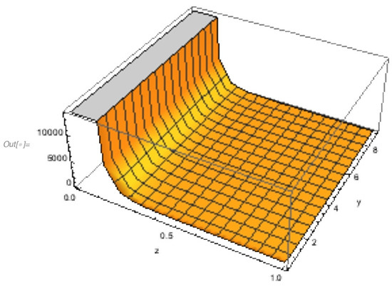
Figure 3. $\tilde{\mu }\equiv 72\pi M^2\mu$ as function of $y\equiv \frac{\alpha }{2}(t-t_0)$ and $z\equiv \frac{r}{r_{\mathsf{\Sigma }}}$ for solution I.

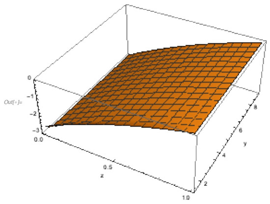
Figure 4. ${\tilde{P}}_r\equiv 72\pi M^2{P}_r$ as function of $y\equiv \frac{\alpha }{2}(t-t_0)$ and $z\equiv \frac{r}{r_{\mathsf{\Sigma }}}$ for solution I.

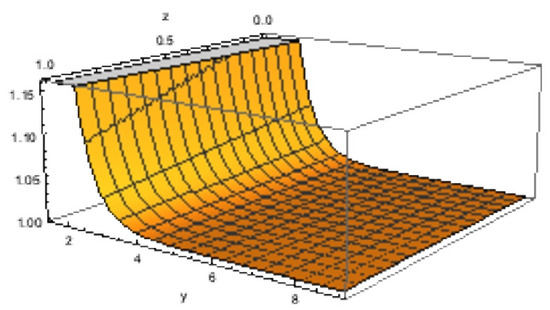
Figure 5. ${\tilde{P}}_{\perp }\equiv 72\pi M^2{P}_{\perp }$ as function of $y\equiv \frac{\alpha }{2}(t-t_0)$ and $z\equiv \frac{r}{r_{\mathsf{\Sigma }}}$ for solution I.

As $t\to \infty$, both solutions tend to the same static solution (97), satisfying a Chaplygin-type equation of state $\mu =-P_r$. The way of reaching this static limit deserves some comments. Usually, the hydrostatic equilibrium is reached when the “gravitational force term” (the first term on the right of (A12)) cancels the “hydrodynamic force term” (the second term on the right of (A12)). However, here, the situation is different: the equilibrium is reached because, as $t\to \infty$, both terms tend to zero. The violent decrease in the “passive gravitational mass” ($\mu +P_r$) is illustrated in Figure 2.

In spite of the good behavior of these two models, it should be mentioned that regularity conditions are not satisfied by the resulting function R on the center of the distribution. Accordingly, for the modeling of any specific scenario, the central region should be excluded.

Next, we considered the case $\omega =0$, which, together with the vanishing complexity factor condition, produces the model $III$. In this model, the boundary areal radius oscillates between 0 and $2M$. The energy density and the tangential pressure of this model are positive and homogeneous, while the radial pressure vanishes identically. As in the previous two models, this solution does not satisfy the regularity condition at the center.

As an additional example of an analytical solution, we considered the case $M=0$. The two models for this type of solution are the models $IV$ and V. They represent a kind of “ghost” star, formed by a fluid distribution not producing gravitational effects outside the boundary surface. They present pathologies, both physical and topological, and therefore their physical applications are dubious. However, since these kinds of distributions have been considered in the past (see, for example, [87]), we present them here.

Next, we considered the subcase where the CKV is orthogonal to the four-velocity and the fluid is dissipative. For this case, we found a model satisfying the vanishing complexity factor and the quasi-homologous condition, which, together with the fulfilment of the matching conditions, determine all of the metric functions. This model (model $VI$) is described by Expressions (137)–(141), and the Expression (147) for the temperature, which has been calculated using the truncated version of the transport equation. It contains contributions from the transient regime (proportional to $\tau$), as well as from the stationary regime. As previous models, this solution does not satisfy the regularity conditions at the center.

The other family of solutions corresponds to the case when the CKV is parallel to the four-velocity. In the non-dissipative case, as a consequence of this symmetry, the metric functions are determined up to three functions (two functions of r and one function of t). In addition, the fluid is necessarily shear-free, a result that was already known [88,89]. The function of t is obtained from the fulfilment of the matching conditions (Equations (153) and (155)). These equations were integrated for different values of the parameters entering into them. Thus, for $a_1=1$ and $ϵ=\frac{1}{27M^2}$, together with the vanishing complexity factor condition and $h\left(r\right)=c_{6}r$, we found model $VII$. The boundary areal radius of this model expands from zero to $3M$, and the physical variables are given by (165)–(167). In the limit $t\to \infty$, the model tends to a static sphere whose equation of state is $P_r=-\mu$. The energy density is positive and presents a singularity only at $t=t_0$; however, regularity conditions are not satisfied at the center.

The integration of the matching conditions for $ϵ=0$ and $a_1=\frac{1}{2}$, together with the vanishing complexity factor, produce the model $VIII$. The boundary areal radius of this model oscillates between zero and $\frac{8M}{3}$. The energy density is positive and larger than the radial pressure, but the fluid distribution is singular at $r=0$.

For $M=0$ and $a_1=1$, we obtain models $IX$ and X. They describe the kind of “ghost stars” mentioned before. However, they are plagued with both physical and topological pathologies that render them unviable for physical modeling. We include them simply for the sake of completeness.

Finally, we considered the dissipative case for the CKV parallel to the four-velocity. The metric variables for this case take the forms (187)–(189), which, after imposing the vanishing complexity factor condition, become (193)–(195). Thus, the metric is determined up to three functions (two functions of t and one function of r). The two functions of t will be obtained from the integration of the matching conditions, whereas the function of r is assumed as (213). The model is further specified with the choice of $a_1=2$. This produce the model $XI$.

As follows from (218), the boundary areal radius of the model tends to infinity as $t\to \infty$, while, in the same limit, the total mass $m_{\mathsf{\Sigma }}$ tends to infinity, whereas both q and $\mu$ tend to zero. The explanation for this strange result arises from the fact that $R_{\mathsf{\Sigma }}$ grows exponentially with t, overcompensating for the decrease in $\mu$ and q in (20). It is also worth noting the negative sign of q, implying an inward heat flux driving the expansion of the fluid distribution.

Overall, we believe that the eleven models exhibited (or at least some of them) could be useful to describe some stages of some regions of self-gravitating fluid in the evolution of compact objects. Each specific scenario imposes specific values on the relevant parameters. It should be reminded that, in any realistic collapsing scenario, we do not expect the same equation of state to be valid all along the evolution and for the whole fluid configuration.

Before concluding, some general comments are in order.

(1)

The analytical integration of the equations derived from the matching conditions have been carried out by imposing specific values on the parameters entering into those equations. In addition, the models have been specified by using some conditions, such as the quasi-homologous condition. Of course, the number of available options is huge. Among them, we would like to mention the prescription of the total luminosity measured by an observer at rest at infinity (36). Let us recall that this is one of the few observables in the process of stellar evolution. Equivalently, one could propose a specific evolution of the total mass with time.

(2)

In some cases where the topological pathologies are not “severe”, the time interval of the viability of the solution may be restricted by the condition that $U\le 1$ (e.g., for solutions I and $II$). In other cases, however, due to topological defects, the interpretation of U as a velocity becomes dubious and therefore it is not clear that U should satisfy the above mentioned condition.

(3)

Model $XI$ is dissipative and intrinsically isotropic in pressure. However, as shown in [71], dissipation produces pressure anisotropy, unless a highly unlikely cancellation of the four terms on the right of Equation (28) in [71] occurs. This happens in model $XI$, which renders this solution a very remarkable one.

(4)

For reasons explained in the Introduction, we have focused on the obtention of analytical solutions expressed through elementary functions. However, it should be clear that, for specific astrophysical scenarios, a numerical approach for solving the matching condition could be more appropriate.

References

- Barenblatt, G.I.; Zeldovich, Y.B. Self-Similar Solutions as Intermediate Asymptotics. Ann. Rev. Fluid. Mech. 1972, 4, 285–312. [Google Scholar] [CrossRef]
- Sedov, L.I. Propagation of strong shock waves. J. Appl. Math. Mech. 1946, 10, 241–250. [Google Scholar]
- Sedov, L.I. Similarity and Dimensional Methods in Mechanics; Academic Press: New York, NY, USA, 1967. [Google Scholar]
- Taylor, G.I. The Formation of a Blast Wave by a Very Intense Explosion. II. The Atomic Explosion of 1945. Proc. Roy. Soc. 1950, 201, 175–186. [Google Scholar]
- Zeldovich, Y.B.; Raizer, Y.P. Physics of Shock Waves and High Temperature; Academic Press: New York, NY, USA, 1963. [Google Scholar]
- Cahill, M.E.; Taub, A.H. Spherically symmetric similarity solutions of the Einstein field equations for a perfect fluid. Commun. Math. Phys. 1971, 21, 1–40. [Google Scholar] [CrossRef]
- Herrera, L.; Jimenez, J.; Leal, L.; Ponce de Leon, J.; Esculpi, M.; Galina, V. Anisotropic fluids and conformal motions in general relativity. J. Math. Phys. 1984, 25, 3274–3278. [Google Scholar] [CrossRef]
- Herrera, L.; Ponce de Leon, J. Isotropic spheres admitting a one parameter group of conformal motions. J. Math. Phys. 1985, 26, 778–784. [Google Scholar] [CrossRef]
- Herrera, L.; Ponce de Leon, J. Anisotropic spheres admitting a one parameter group of conformal motions. J. Math. Phys. 1985, 26, 2018–2023. [Google Scholar] [CrossRef]
- Herrera, L.; Ponce de Leon, J. Isotropic and anisotropic charged spheres admitting a one parameter group of conformal motions. J. Math. Phys. 1985, 26, 2302–2307. [Google Scholar] [CrossRef]
- Herrera, L.; Ponce de Leon, J. Confined gravitational fields produced by anisotropic spheres. J. Math. Phys. 1985, 26, 2847–2849. [Google Scholar] [CrossRef]
- Maartens, R.; Mason, P.S.; Tsamparlis, M. Kinematic and dynamic properties of conformal Killing vectors in anisotropic fluids. J. Math. Phys. 1986, 27, 2987–2994. [Google Scholar] [CrossRef]
- Duggal, K.L.; Sharma, R. Conformal collineations and anisotropic fluids in general relativity. J. Math. Phys. 1986, 27, 2511–2513. [Google Scholar] [CrossRef]
- Esculpi, M.; Herrera, L. Conformally symmetric radiating spheres in general relativity. J. Math. Phys. 1986, 27, 2087–2096. [Google Scholar] [CrossRef]
- Duggal, K.L. Relativistic fluids with shear and timelike conformal collineations. J. Math. Phys. 1987, 28, 2700–2704. [Google Scholar] [CrossRef]
- Mason, D.P.; Maartens, R. Kinematics and dynamics of conformal collineations in relativity. J. Math. Phys. 1987, 28, 2182–2186. [Google Scholar] [CrossRef]
- Di Prisco, A.; Herrera, L.; Jimenez, J.; Galina, V.; Ibanez, J. The Bondi metric and conformal motions. J. Math. Phys. 1987, 28, 2692–2696. [Google Scholar] [CrossRef]
- Duggal, K.L. Relativistic fluids and metric symmetries. J. Math. Phys. 1989, 30, 1316–1322. [Google Scholar] [CrossRef]
- Coley, A.A.; Tupper, B.O.J. Special conformal Killing vector space-times and symmetry inheritance. J. Math. Phys. 1989, 30, 261–2625. [Google Scholar] [CrossRef]
- Coley, A.A.; Tupper, B.O.J. Spacetimes admitting inheriting conformal Killing vector fields. Class. Quantum Grav. 1990, 7, 1961–1981. [Google Scholar] [CrossRef]
- Coley, A.A.; Tupper, B.O.J. Spherically symmetric spacetimes admitting inheriting conformal Killing vector fields. Class. Quantum Grav. 1990, 7, 2195–2214. [Google Scholar] [CrossRef]
- Maartens, R.; Maharaj, M.S. Conformally symmetric static fluid spheres. J. Math. Phys. 1990, 31, 151–155. [Google Scholar] [CrossRef]
- Di Prisco, A.; Herrera, L.; Esculpi, M. Self-similar scalar soliton star in the thin wall approximation. Phys. Rev. D 1991, 44, 2286–2294. [Google Scholar] [CrossRef] [PubMed]
- Saridakis, E.; Tsamparlis, M. Symmetry inheritance of conformal Killing vectors. J. Math. Phys. 1991, 32, 1541–1551. [Google Scholar] [CrossRef]
- Aguirregabiria, J.M.; Di Prisco, A.; Herrera, L.; Ibanez, J. Time evolution of self–similar scalar soliton stars: A general study. Phys. Rev. D 1992, 46, 2723–2725. [Google Scholar] [CrossRef] [PubMed]
- Maartens, R.; Maharaj, S.D.; Tupper, B.O.J. General solution and classification of conformal motions in static spherical spacetimes. Class. Quantum Grav. 1995, 12, 2577–2586. [Google Scholar] [CrossRef]
- Maharaj, S.D.; Maartens, R.; Maharaj, M.S. Conformal symmetries in static spherically symmetric spacetimes. Int. J. Theor. Phys. 1995, 34, 2285–222901. [Google Scholar] [CrossRef]
- Carot, J.; Sintes, A. Homothetic perfect fluid spacetimes. Class. Quantum Grav. 1997, 14, 1183–1205. [Google Scholar] [CrossRef]
- Carr, B.J.; Coley, A.A. TOPICAL REVIEW: Self-similarity in general relativity. Class. Quantum Grav. 1999, 16, R31–R71. [Google Scholar] [CrossRef]
- Barreto, W.; da Silva, A. Self-similar and charged spheres in the diffusion approximation. Class. Quantum Grav. 1999, 16, 1783–1792. [Google Scholar] [CrossRef][Green Version]
- Yavuz, I.; Yilmaz, I.; Baysal, H. Strange Quark Matter Attached to the String Cloud in the Spherical Symmetric Space-Time Admitting Conformal Motion. Int. J. Mod. Phys. D 2005, 14, 1365–1372. [Google Scholar] [CrossRef]
- Sharif, M.; Sheikh, U. Timelike and Spacelike Matter Inheritance Vectors in Specific Forms of Energy-Momentum Tensor. Int. J. Mod. Phys. A 2006, 21, 3213–3234. [Google Scholar] [CrossRef]
- Barreto, W.; Rodriguez, B.; Rosales, L.; Serrano, O. Self–similar and charged radiating spheres: An anisotropic approach. Gen. Relativ. Gravit. 2007, 39, 23–39. [Google Scholar] [CrossRef]
- Mak, M.K.; Harko, T. Quark stars admitting a one parameter group of conformal motions. Int. J. Mod. Phys. D 2004, 13, 149–156. [Google Scholar] [CrossRef]
- Moopanar, S.; Maharaj, S.D. Conformal symmetries of spherical spacetimes. Int. J. Theor. Phys. 2010, 49, 1878–1885. [Google Scholar] [CrossRef][Green Version]
- Bhar, P. Vaydya–Tikekar–type superdense star admitting conformal motion in presence of quintessence field. Eur. Phys. J. C 2015, 75, 123. [Google Scholar] [CrossRef]
- Apostolopoulos, P.S. Spatially inhomogeneous and irrotational geometries admitting intrinsic conformal symmetries. Phys. Rev. D 2016, 94, 124052. [Google Scholar] [CrossRef]
- Shee, D.; Rahaman, F.; Guha, B.K.; Ray, S. Anisotropic stars with non–static conformal symmetry. Astr. Space Sci. 2016, 361, 167. [Google Scholar] [CrossRef]
- Majonjo, A.; Maharaj, S.D.; Moopanar, S. Conformal vectors and stellar models. Eur. Phys. J. Plus 2017, 132, 62. [Google Scholar] [CrossRef]
- Newton Singh, K.; Murad, M.; Pant, N. A 4D spacetime embedded in a 5D pseudo–Euclidean space describing interior compact stars. Eur. Phys. J. A 2017, 53, 21. [Google Scholar] [CrossRef]
- Shee, D.; Deb, D.; Ghosh, S.; Guha, B.K.; Ray, S. On the features of Matese–Whitman mass fucntion. arXiv 2017, arXiv:1706.00674. [Google Scholar]
- Herrera, L.; Di Prisco, A. Self–similarity in static axially symmetric relativistic fluid. Int. J. Mod. Phys. D 2018, 27, 1750176. [Google Scholar] [CrossRef]
- Ojako, S.; Goswami, R.; Maharaj, S.D. New class of solutions in conformally symmetric massless scalar field collapse. Gen. Relativ. Gravit. 2021, 53, 13. [Google Scholar] [CrossRef]
- Shobhane, P.; Deo, S. Spherically symmetric distributions of wet dark fluid admitting conformal motions. Adv. Appl. Math. Sci. 2021, 20, 1591–1598. [Google Scholar]
- Jape, J.; Maharaj, S.D.; Sunzu, J.; Mkenyeleye, J. Generalized compact star models with conformal symmetry. Eur. Phys. J. C 2021, 81, 2150121. [Google Scholar] [CrossRef]
- Ivanov, B. Generating solutions for charged stellar models in general relativity. Eur. Phys. J. C 2021, 81, 227. [Google Scholar] [CrossRef]
- Sherif, A.; Dunsby, P.; Goswami, R.; Maharaj, S.D. On homothetic Killing vectors in stationary axisymmetric vacuum spacetimes. Int. J. Geom. Meth. Mod. Phys. 2021, 18, 21550121. [Google Scholar] [CrossRef]
- Matondo, D.; Maharaj, S.D. A Tolman–like Compact Model with Conformal Geometry. Entropy 2021, 23, 1406. [Google Scholar] [CrossRef]
- Bhar, P.; Rej, P. Stable and self–consistent charged gravastar model within the framework of f(R,T) gravity. Eur. Phys. J. C 2021, 81, 763. [Google Scholar] [CrossRef]
- Sharma, R. Proper special conformal Killing vectors and the quadratic theory of gravity. J. Math. Phys. 1991, 32, 1854. [Google Scholar] [CrossRef]
- Mak, M.K.; Harko, T. Can the galactic rotation curves be explained in brane world models? Phy. Rev. D 2004, 70, 024010. [Google Scholar] [CrossRef]
- Harko, T.; Mak, M.K. Conformally symmetric vacuum solutions of the gravitational field equations in the brane world model. Ann. Phys. 2005, 319, 471–492. [Google Scholar] [CrossRef]
- Sharif, M.; Fatima, H.I. Static spherically symmetric solutions in f(G) gravity. Int. J. Mod. Phys. D 2016, 25, 1650083. [Google Scholar] [CrossRef]
- Sefiedgar, A.S.; Haghani, Z.; Sepangi, H.R. Brane f(R) gravity and dark matter. Phy. Rev. D 2012, 85, 064012. [Google Scholar] [CrossRef]
- Bhar, P. Higher dimensional charged gravastar admitting conformal motion. Astrophys. Space Sci. 2014, 354, 457–462. [Google Scholar] [CrossRef]
- Turkoglu, M.; Dogru, M. Conformal cylindrically symmetric spacetimes in modified gravity. Mod. Phys. Lett. A 2015, 30, 1550202. [Google Scholar] [CrossRef]
- Das, A.; Rahaman, F.; Guha, B.K.; Ray, S. Relativistic compact stars in f(T) gravity admitting conformal motion. Astrophys. Space Sci. 2015, 358, 36. [Google Scholar] [CrossRef]
- Sert, O. Radiation fluid stars in the non–minimally coupled Y(R)F2 gravity. arXiv 2016, arXiv:1611.03821v1. [Google Scholar]
- Zubair, M.; Sardar, L.H.; Rahaman, F.; Abbas, G. Interior solutions for fluid spheres in f(R,T) gravity admitting conformal killing vectors. Astrophys. Space Sci. 2016, 361, 238. [Google Scholar] [CrossRef]
- Das, A.; Rahaman, F.; Guha, B.K.; Ray, S. Compact stars in f(R,T) gravity. Eur. Phys. J. C 2016, 76, 654. [Google Scholar] [CrossRef]
- Sharif, M.; Naz, S. Stable charged gravastar model in f(R,T2) gravity with conformal motion. Eur. Phys. J. P. 2022, 137, 421. [Google Scholar] [CrossRef]
- Bohmer, C.G.; Harko, T.; Lobo, F.S.N. Conformally traversable wormholes. Phys. Rev. D 2007, 76, 084014. [Google Scholar] [CrossRef]
- Bohmer, C.G.; Harko, T.; Lobo, F.S.N. Wormhole geometries with conformal motions. Class. Quantum Grav. 2008, 25, 075016. [Google Scholar] [CrossRef]
- Rahaman, F.; Ray, S.; Khadekar, G.; Kuhfittig, P.; Karakar, I. Noncommutative geometry inspired wormholes with conformal motion. Int. J. Theor. Phys. 2015, 54, 699–709. [Google Scholar] [CrossRef]
- Kuhfittig, P. Wormholes admitting conformal Killing vectors and supported by generalized Chaplygin gas. Eur. Phys. J. C 2015, 75, 357. [Google Scholar] [CrossRef]
- Sharif, M.; Fatima, H.I. Conformally symmetric traversable wormhole in f(G) gravity. Gen. Relativ. Gravit. 2016, 48, 148. [Google Scholar] [CrossRef]
- Kar, S. Curious variant of the Bronnikov–Ellis spacetime. Phys. Rev. D 2022, 105, 024013. [Google Scholar] [CrossRef]
- Mustafa, G.; Hassan, Z.; Sahoo, P.K. Traversable wormhole inspired by non–commutative geometries in f(Q) gravity with conformal symmetry. Ann. Phys. 2022, 437, 168751. [Google Scholar] [CrossRef]
- Herrera, L.; Di Prisco, A.; Ospino, J. Quasi–homologous evolution of self–gravitating systems with vanishing complexity factor. Eur. Phys. J. C 2020, 80, 631. [Google Scholar] [CrossRef]
- Herrera, L.; Santos, N.O. Local anisotropy in self–gravitating systems. Phys. Rep. 1997, 286, 53–130. [Google Scholar] [CrossRef]
- Herrera, L. Stabilty of the isotropic pressure condition. Phys. Rev. D 2020, 101, 104024. [Google Scholar] [CrossRef]
- Herrera, L. New definition of complexity for self–gravitating fluid distributions: The spherically symmetric case. Phys. Rev. D 2018, 97, 044010. [Google Scholar] [CrossRef]
- Herrera, L.; Di Prisco, A.; Ospino, J. Definition of complexity for dynamical spherically symmetric dissipative self–gravitating fluid distributions. Phys. Rev. D 2018, 98, 104059. [Google Scholar] [CrossRef]
- Herrera, L.; Ospino, J.; Di Prisco, A.; Fuenmayor, E.; Troconis, O. Structure and evolution of self–gravitating objects and the orthogonal splitting of the Riemann tensor. Phys. Rev D 2009, 79, 064025. [Google Scholar] [CrossRef]
- Herrera, L.; Di Prisco, A.; Ibáñez, J. Tilted Lemaitre–Tolman–Bondi spacetimes: Hydrodynamic and thermodynamic properties. Phys. Rev. D 2011, 84, 064036. [Google Scholar] [CrossRef]
- Chan, R. Collapse of a radiating star with shear. Mon. Not. R. Astron. Soc. 1997, 288, 589–595. [Google Scholar] [CrossRef]
- Israel, W. Nonstationary irreversible thermodynamics: A causal relativistic theory. Ann. Phys. 1976, 100, 310–331. [Google Scholar] [CrossRef]
- Israel, W.; Stewart, J. Thermodynamic of nonstationary and transient effects in a relativistic gas. Phys. Lett. A 1976, 58, 213–215. [Google Scholar] [CrossRef]
- Israel, W.; Stewart, J. Transient relativistic thermodynamics and kinetic theory. Ann. Phys. 1979, 118, 341–372. [Google Scholar] [CrossRef]
- Triginer, J.; Pavon, D. On the thermodynamics of tilted and collisionless gases in Friedmann–Robertson–Walker spacetimes. Class. Quantum Grav. 1995, 12, 199. [Google Scholar] [CrossRef]
- Schwarzschild, M. Structure and Evolution of the Stars; Dover: New York, NY, USA, 1958. [Google Scholar]
- Kippenhahn, R.; Weigert, A. Stellar Structure and Evolution; Springer: Berlin/Heidelberg, Germany, 1990. [Google Scholar]
- Hansen, C.; Kawaler, S. Stellar Interiors: Physical Principles, Structure and Evolution; Springer: Berlin/Heidelberg, Germany, 1994. [Google Scholar]
- Stephani, H.; Kramer, D.; MacCallum, M.; Honselaers, C.; Herlt, E. Exact Solutions to Einstein Field Equations, 2nd ed; Cambridge University Press: Cambridge, UK, 2003. [Google Scholar]
- Carot, J. Some developments on axial symmetry. Class. Quantum Grav. 2000, 17, 2675. [Google Scholar] [CrossRef]
- Carlson, G.T., Jr.; Safko, J.L. Canonical forms for axial symmetric space–times. Ann. Phys. 1980, 128, 131–153. [Google Scholar] [CrossRef]
- Zeldovich, Y.B.; Novikov, I.D. Relativistic Astrophysics; The University of Chicago Press: Chicago, IL, USA, 1971. [Google Scholar]
- Oliver, D.R., Jr.; Davis, W.R. On certain timelike symmetry properties and the evolution of matter field space–times that admit them. Gen. Rel. Grav. 1977, 8, 905–914. [Google Scholar] [CrossRef]
- Herrera, L.; Di Prisco, A.; Ibanez, J. Reversible dissipative processes, conformal motions and Landau damping. Phys. Lett. A 2012, 376, 899–900. [Google Scholar] [CrossRef]
Publisher’s Note: MDPI stays neutral with regard to jurisdictional claims in published maps and institutional affiliations. |
© 2022 by the authors. Licensee MDPI, Basel, Switzerland. This article is an open access article distributed under the terms and conditions of the Creative Commons Attribution (CC BY) license (https://creativecommons.org/licenses/by/4.0/).