Spectral Instability in Modified Pöschl–Teller Effective Potential Triggered by Deterministic and Random Perturbations

Abstract

Owing to its substantial implications for black hole spectroscopy, spectral instability has attracted considerable attention in the literature. While the emergence of such instability is attributed to the non-Hermitian nature of the gravitational system, it remains sensitive to various factors. In this work, we conduct a focused analysis of black hole spectral instability using the Pöschl–Teller potential as a toy model. We investigate the dependence of the resulting spectral instability on the magnitude, spatial scale, and localization of deterministic and random perturbations in the effective potential of the wave equation, and discuss the underlying physical interpretations. It is observed that small perturbations in the potential initially have a limited impact on the less damped black hole quasinormal modes, with deviations typically around their unperturbed values, a phenomenon first derived by Skakala and Visser in a more restrictive context. In the higher-overtone region, the deviation propagates, amplifies, and eventually gives rise to spectral instability and, inclusively, bifurcation in the quasinormal mode spectrum. While deterministic perturbations give rise to a deformed but well-defined quasinormal spectrum, random perturbations lead to uncertainties in the resulting spectrum. Nonetheless, the primary trend of the spectral instability remains consistent, being sensitive to both the strength and location of the perturbation. However, we demonstrate that the observed spectral instability might be suppressed for perturbations that are physically appropriate.

1. Introduction

Black holes are among the most intriguing concepts in theoretical physics. They exemplify gravity’s properties at their extremity through an elegant and concise mathematical framework. The success of the ground-based LIGO and Virgo collaborations in capturing gravitational waves emanating from binary mergers [1,2,3,4], as well as ongoing spaceborne projects, such as LISA [5], TianQin [6], and Taiji [7], marks the inauguration of a new epoch for observational astrophysics. In particular, the feasibility of direct observation of ringdown waveforms has also been explored [8].

The black hole ringdown waveform is primarily determined by a linear combination of quasinormal modes (QNMs) [9,10], whose study has sparked considerable interest. It is well-known [11,12] that, in the frequency space, QNMs can be attributed to the poles of the Green’s function related to the master wave equation, whereas the late-time behavior is associated with the branch cut, which typically corresponds to an exponential decay followed by an inverse power tail in the time domain [13]. Along this line of thought, it has been understood in the literature that the unique characteristic of QNMs, determined solely by the spacetime properties surrounding the black hole, provides unambiguous information about the spacetime geometry near the event horizon.

However, to some extent, this concept has been challenged recently by the renewed discussion of spectral instability [14,15,16,17,18,19]. Pioneered by Nollert and Price [14,15], it was shown that even minor perturbations in the Regge–Wheeler potential, such as step functions, can significantly influence the higher-overtone modes in the QNM spectrum, demonstrating an unexpected instability of the QNM spectrum against small-scale perturbations. This finding challenges the conventional assumption that a reasonable approximation of the effective potential is expected to result in only minimal deviation in the resulting QNMs. Further analytic and numerical studies [16,17] have indicated that even in the presence of discontinuities of a more moderate nature, the asymptotic behavior of the QNM spectrum could be non-perturbatively modified. Specifically, high-overtone modes might shift along the real frequency axis rather than ascending the imaginary frequency axis observed for most black hole metrics [20,21]. It was argued that this feature persists regardless of the discontinuity’s distance from the horizon or its magnitude. Generalizing these results, Jaramillo et al. [18] explored the topic in terms of the notion of spectral instability. Their analyses revealed that the boundary of the pseudospectrum moves closer to the real frequency axis, thus reinforcing the notion of a universal instability of high-overtone modes triggered by “ultraviolet,” meaning small-scale, perturbations.

Because in a real-world astrophysical context gravitational radiation sources such as black holes are hardly isolated objects, the above results have an immediate and substantial implication in black hole spectroscopy, which involves modeling of black hole waveforms and extracting the underlying metric parameters, inclusively involving the temporal profiles dominated by QNMs [22,23,24,25,26,27,28,29]. The fact that black holes are typically submerged and interact with the surrounding matter leads to deviations from the ideal symmetric metric. As a result, the emitted gravitational waves of the underlying QNMs might differ substantially from those predicted for a pristine, isolated, compact object. In the literature, such phenomena have motivated the investigation into “dirty” black holes, as explored by several authors [30,31,32,33], and opened new avenues in the study of black hole perturbation theory. Moreover, the asymptotic modes that align almost parallel to the real axis are closely related to the intriguing concept of echoes, a late-stage ringing waveform first proposed by Cardoso et al. [34,35]. As potential observables, echoes might help distinguish different but otherwise similar gravitational systems via their distinct properties near the horizon. This idea has spurred many studies into echoes across various systems, encompassing exotic compact objects such as gravastars and wormholes. Like the late-time tail, echoes are also attributed to the analytic properties of Green’s function, as analyzed by Mark et al. [36]. In studies of Damour–Solodukhin-type wormholes [37], Bueno et al. [38] have investigated echoes by explicitly solving for specific frequencies at which the transition matrix becomes singular, providing further insights into the complex interplay of spacetime geometry and QNMs. For the above scenarios, the perturbations in the effective potential are not necessarily located close to the event horizon. In other words, the apparent deformation in the frequency-space QNM spectrum, and potentially the consequential time-domain waveforms, might not be entirely attributed to the distortion of the spacetime curvature near the compact object in question.

The related topic of spectral instability, echoes, greybody factor, and causality has been extensively explored in recent years by many authors [39,40,41,42,43,44,45,46,47,48,49,50,51,52,53,54,55,56,57,58,59,60,61,62,63] (see [19] for a more comprehensive list of references). Notably, Cheung et al. [42] pointed out that even the fundamental mode can be destabilized under generic perturbations. By introducing a small perturbation to the Regge–Wheeler effective potential, it was shown [42] that the fundamental mode undergoes an outward spiral while the deviation’s magnitude increases. Subsequently, its position is overtaken by a new mode distinct from the first few low-lying modes. The results have been ascertained using different shapes for a small bump in the potential and observed in a toy model constituted by two disjointed rectangular potential barriers [42,51] and derived from an analytic account [54,55,64,65]. Further analysis revealed that the fundamental mode can remain stable, depending sensitively on the specific background metric and perturbations [54]. The observed interplay between the fundamental mode and echo modes can also be properly assessed [60]. Although it has been argued that spectral instability might not significantly impact the time-domain waveform [43], these observations potentially undermine the feasibility of black hole spectroscopy as the fundamental mode is shown to be subjected to spectral instability. Besides the scale of the perturbation, the above findings indicate that its location is also relevant. In this regard, a systematic analysis of the change in the spectrum in relation to different characteristics of perturbations in the potential is still lacking in the literature.

The present study is motivated by the above considerations. Our analysis focuses on the sensitivity of the QNM spectrum against the magnitude, spatial scale, and localization of the perturbations in different effective potentials. To this end, we consider the theoretical setup that the study of black hole perturbations can be simplified by exploring the spatial part of the master equation [10],

$$\begin{array}{c}\hfill {\displaystyle \frac{{\partial }^2}{\partial t^2}}\mathrm{\Psi }(t,r_{\ast })+\left(-{\displaystyle \frac{{\partial }^2}{\partial r_{\ast }^2}}+V_{\mathrm{eff}}\right)\mathrm{\Psi }(t,r_{\ast })=0,\end{array}$$

(1)

where $r_{\ast }$ is the tortoise coordinate, and $V_{\mathrm{eff}}$ is the effective potential determined by the spacetime metric, spin $\overline{s}$, and angular momentum ℓ of the perturbation. For instance, the Pöchl–Teller potential is given by

$$V_{\mathrm{PT}}\equiv V_0{\mathrm{sech}}^2\left({\displaystyle \frac{r_{\ast }}{b}}\right),$$

(2)

where $V_0$ and b are two parameters governing the shape of the potential.

The quasinormal frequencies can be obtained by evaluating the zeros of the Wronskian,

$$\begin{array}{c}\hfill W\left(\omega \right)\equiv W(g,f)=g(\omega ,r_{\ast })f^{\prime }(\omega ,r_{\ast })-f(\omega ,r_{\ast })g^{\prime }(\omega ,r_{\ast }),\end{array}$$

(3)

where ′ $\equiv d/d{r}_{\ast }$, and f and g are the solutions of the corresponding homogeneous equation of Equation (1) in the frequency domain [9],

$$\begin{array}{c}\hfill \left[-{\omega }^2-{\displaystyle \frac{d^2}{d{r}_{\ast }^2}}+V_{\mathrm{eff}}\right]\tilde{\mathrm{\Psi }}(\omega ,r_{\ast })=0,\end{array}$$

(4)

with appropriate boundary conditions, namely,

$$\begin{array}{c}\hfill \begin{array}{cc}f(\omega ,r_{\ast })\sim e^{-i\omega r_{\ast }}& r_{\ast }\to -\infty ,\\ \\ g(\omega ,r_{\ast })\sim e^{i\omega r_{\ast }}& r_{\ast }\to +\infty .\end{array}\end{array}$$

(5)

As discussed above, the present paper aims to analyze the impact of different forms of perturbations in the effective potential on the resulting QNM spectrum. These perturbations can be interpreted as resulting from perturbations in the spacetime metric. However, instead of deriving the modified effective potential from physically relevant metric perturbations, we introduce the perturbation directly into the effective potential $V_{\mathrm{eff}}$, following a practice commonly adopted by other authors [14,18,42]. The main motivation for this approach is mathematical simplicity, which enables us to focus on the essential features of the spectral instability. We note that the physical relevance of such perturbations in the potential is an important issue that has been highlighted by other authors [53].

The remainder of the paper is organized as follows. In Section 2, we start our analysis with deterministic perturbations in the Pöschl–Teller potential, from which we discuss the resulting impact on the QNM spectrum and spectral instability. The dependence of the change in the spectrum on the magnitude and frequency of the perturbation in the effective potential is explored. In Section 3, we further analyze the case where the perturbation possesses an arbitrary shape. Subsequently, we elaborate on the scenario in which a small-scale perturbation is introduced to the effective potential and investigate the effect of its location in Section 4. The last section includes further discussions and concluding remarks. In this study, numerical calculations are carried out using the matrix method [66], which has been verified by repeating the calculations with different grid sizes and precisions.

2. Spectral Instability Triggered by Deterministic Perturbations

We consider the perturbed Pöschl–Teller potential of the following form

$$V_{\mathrm{eff}}=V_{\mathrm{PT}}+V_{\mathrm{pert}},$$

(6)

where we assume the parameters $V_0=b=5$ for the Pöschl–Teller potential Equation (2). The quasinormal frequencies of the original Pöchl–Teller potential are given by [67]

$${\omega }_n^{\mathrm{PT}}=\sqrt{V_0-{\displaystyle \frac{1}{4b^2}}}-i{\displaystyle \frac{1}{b}}\left(n+{\displaystyle \frac{1}{2}}\right),$$

(7)

which implies that $\mathrm{Re}{\omega }_n\sim 2.23383$ and a constant distance of $0.2$ along the imaginary axis between successive modes, for the given parameters. For the deterministic case, the perturbation takes the form

$$V_{\mathrm{pert}}=V_{\mathrm{pert}}^{\det }=ϵsin\left(k\pi x\right),$$

(8)

where the magnitude $ϵ$ and wave number k will be tuned in our calculations to the compactified coordinate

$$\begin{array}{c}\hfill x=tanh\left(r_{\ast }\right).\end{array}$$

(9)

Regarding the specific form of Equation (8), some comments are in order. As pointed out in [18], the QNM spectrum is sensitive to small-scale perturbations. The parameterization of Equation (8) features an explicit dependence on the perturbation’s spatial scale via the parameter k. Secondly, when transformed from the compactified coordinate x to the tortoise coordinate $r_{\ast }$, this perturbation is exponentially suppressed at the bound $x=\pm 1$. Specifically, as $r_{\ast }\to \pm \infty$ we have $x\sim \pm \left[1-2exp(-2|r_{\ast }\left|\right)\right]$, and subsequently,

$$|V_{\mathrm{pert}}^{\det }|\sim 2ϵk\pi exp(-2|r_{\ast }\left|\right)\ll V_{0}exp(-2|r_{\ast }|/b)\sim V_{\mathrm{PT}},$$

given $b\ge 1$ and $ϵk\ll V_0$. In other words, this perturbation is minor in size compared to the original black hole potential.

The calculations are performed using the matrix method [66]. This approach reformulates the master equation for QNMs into an algebraic one for complex eigenvalues. By mapping the physical coordinate domain onto a compact interval and factoring out the asymptotic behavior of the wavefunction, the remaining part becomes regular across the interval, allowing the boundary conditions to be imposed as simple vanishing values. With a suitable field redefinition and grid discretization, the differential equation is transformed into a matrix equation. The quasinormal frequencies are then obtained as the eigenvalues of a generalized matrix eigenvalue problem, which can be efficiently solved using standard numerical algorithms. In the present study, we adopt a recent version of the matrix method, which is implemented in hyperboloidal coordinates [68,69] on a Chebyshev grid [70]. The precision and consistency of the numerical results are ensured by repeating the calculations using different grid sizes.

In Figure 1, we show the effect of the spatial scale of the perturbation, in terms of the wave number k. It is observed that the deviation of the QNM spectrum initiates from the high overtones and propagates towards the low-lying modes. For small wave numbers, the deviations oscillate around their unperturbed values (governed by Equation (7)). As the spatial scale decreases, the amplitude of such deviation increases rapidly. Specifically, even though the deviations associated with $k=1.0$ indicated by the empty blue squares are clearly identified in the top-left panel, they become almost invisible when presented in the top-right panel, when compared against the deviation triggered by the wave number $k=2.0$, shown in empty orange diamonds. The latter again becomes insignificant when compared with the deviation represented by empty black triangles for $k=2.0$ shown in the middle-left panel. In all three panels, the deviations oscillate around the unperturbed QNM spectrum, with higher overtones experiencing more significant deviations. Moreover, as the wave number increases further, a bifurcation point emerges, and the resulting QNM spectrum divides into two different branches. The instability continues to propagate towards the low overtones. It is intriguing to note that such a phenomenon is reminiscent of what was first observed by Skakala and Visser [71,72], and was subsequently explored in the context of spectral instability in [69]. However, these existing studies are in a somewhat different and more restrictive context for small-scale perturbations featuring a discontinuity.

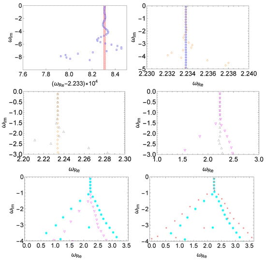
Figure 1. The spectral instability in the modified Pöschl–Teller effective potential Equation (6) triggered by a deterministic perturbation Equation (8), where one assumes $V_0=b=5$ and $ϵ=0.001$. From left to right and top to bottom, we compare in pairs the resulting QNM spectra for different perturbations using the wave numbers $k=0$ (unperturbed potential, empty red circles), $1.0$ (empty blue squares), $2.0$ (empty orange diamonds), $3.0$ (empty gray triangles), $4.0$ (empty magenta flipped triangles), $5.0$ (filled cyan circles), and $6.0$ (filled pink squares). The numerical calculations are carried out using the matrix method, and the results have been verified using different grid sizes.

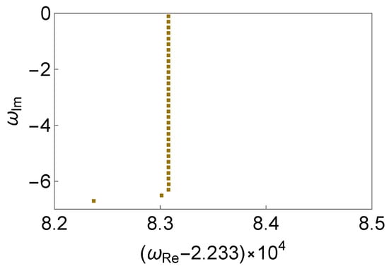
In Figure 2, we study the effect of the magnitude of the perturbation, in terms of the parameter $ϵ$. Again, the numerical results obtained by the matrix method have been ascertained using different grid sizes. The deformation of the QNM spectrum initiates from the high overtones and propagates towards the low-lying modes. As the magnitude of the perturbation gradually increases and exceeds a particular value (in our specific case, $ϵ\gtrsim 1\times {10}^{-4}$), a bifurcation can be clearly identified. The bifurcation causes a division of two branches of QNM spectra leaning towards opposite directions. As the magnitude increases further, the bifurcation propagates towards the low-lying modes, leading to a more significant distortion of the QNM spectrum. Moreover, as shown in the bottom-right panel, the branch which leans towards the imaginary frequency axis is found to turn into purely imaginary modes. We note that this feature is similar to the imaginary modes observed in [69]. Different from [69], where these modes can be confirmed by explicitly evaluating the Wronskian and derived analytically under reasonable approximation, here the results are numerical for the most part, and can only be obtained using an approach based on explicit evaluations of the perturbed effective potential. In practice, it is known that imaginary modes can be merely a numerical artifact. Therefore, the claim of their existence (c.f. the special algebraic mode derived by Chandrasekhar [73]) must be confirmed with extra caution. However, based on the strong resemblance between the present results and those derived in [69], we speculate that the formation of a series of purely imaginary modes in the modified Pöschl–Teller effective potential is a general result.

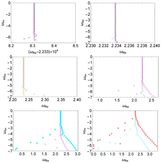
Figure 2. The spectral instability in the modified Pöschl–Teller effective potential Equation (6) triggered by deterministic perturbations Equation (8), where one assumes $V_0=b=5$ and $k=3.0$. From left to right and top to bottom, we compare in pairs the resulting QNM spectra for different perturbations using the magnitudes $ϵ=1\times {10}^{-8}$ (empty red circles), $1\times {10}^{-7}$ (empty blue squares), $1\times {10}^{-6}$ (empty orange diamonds), $1\times {10}^{-5}$ (empty gray triangles), $1\times {10}^{-4}$ (empty magenta flipped triangles), $1\times {10}^{-3}$ (filled cyan circles), and $1\times {10}^{-2}$ (filled pink circles). The numerical calculations are carried out using the matrix method, and the results have been verified using different grid sizes.

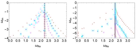
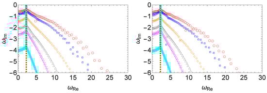
In Figure 3, we summarize all the spectra presented in Figure 1 and Figure 2. From a more general perspective, we see that the spectral instability is more susceptible to more significant, as well as small-scale perturbations, as first pointed out in [18]. A closer analysis indicates that for both large wave numbers and magnitudes, a bifurcation is observed in the spectrum, which propagates from high overtones to the low-lying ones (c.f. Figure 7 of [18]). For an overtone of a given order, the deviation becomes more significant as the wave number or magnitude of the perturbation increases. On the other hand, for perturbations of relatively small wave numbers, there is no bifurcation, and the deviation oscillates. Both features have been observed in the Pöschl–Teller effective potential [69], where the perturbation was implemented by introducing some discontinuity in terms of a cut or step, and a semi-analytic derivation was feasible. For the present case, there is no discontinuity, and we speculate that such features are rather general.

Figure 3. A summary of the changes in the QNM spectra shown in Figure 1 (left) and Figure 2 (right).

3. Spectral Instability Triggered by Random Perturbations

Now we proceed to analyze random perturbations subject to the two following forms First, we consider the case

$$V_{\mathrm{pert}}=V_{\mathrm{pert}}^{\mathrm{ran}}=x\epsilon ,$$

(10)

where $\epsilon$ measures the strength and x is governed by a probability density function $g\left(r\right)$, such that $P(r\le R<r+dr)\approx g\left(r\right)dr$. Here, we consider the contribution to be a uniform distribution with $-1\le x\le 1$, giving rise to a uniform white noise satisfying

$$X\sim WN\left(0,{\sigma }^2={\displaystyle \frac{1}{3}}\right).$$

(11)

It is noted that the random perturbations governed by Equation (10) are implemented in a pointwise fashion. Specifically, at individual spatial coordinate points, the magnitude $\epsilon$ will receive a rescaling governed by the random variable X, whose value is determined entirely independently from those applied to other positions.

The results are shown in Figure 4, where the resulting QNM spectra are evaluated for perturbations featuring white noise of different magnitudes. Owing to the nature of randomness, for a perturbation of a given strength, the modified QNM spectra, particularly the high overtones, will vary. This is why we present multiple results for given configurations. Nonetheless, a consistent trend is observed and, in particular, the low overtones remain essentially unchanged. It is somewhat surprising that spectral instability is observed at a minimal level of “random noise” in the effective potential. As shown in the bottom-right panel of Figure 4, even for the magnitude $\epsilon =1\times {10}^{-30}$, a bifurcation is manifestly shown around $\mathrm{Im}{\omega }_n\simeq -4$, and a significant change in the spectrum is observed for higher overtones. As the strength of the perturbation increases, the deviation propagates from high overtones toward the low-lying ones.

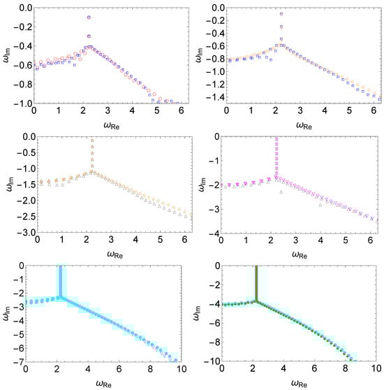
Figure 4. The spectral instability in the modified Pöschl–Teller effective potential Equation (6) triggered by a random perturbation Equation (10), where one assumes $V_0=b=5$. For random perturbations of a given strength, two sets of results are presented in each panel. From left to right and top to bottom, we show the resulting QNM spectra for different perturbations using the magnitudes $\epsilon =1\times {10}^{-3}$ (empty red circles and empty blue squares), $1\times {10}^{-5}$ (empty blue squares and empty orange diamonds), $1\times {10}^{-10}$ (empty orange diamonds and empty gray triangles), $1\times {10}^{-15}$ (empty gray triangles and empty magenta flipped triangles), $1\times {10}^{-20}$ (empty magenta flipped triangles and filled cyan circles), $1\times {10}^{-30}$ (filled cyan circles and filled dark-yellow squares). Due to the nature of the random perturbation, the modified QNM spectra, particularly the high overtones, do not coincide precisely, even though a consistent trend is observed. The numerical calculations are carried out using the matrix method.

Secondly, we explore an interplay between random and deterministic perturbations by considering the case

$$V_{\mathrm{pert}}=V_{\mathrm{pert}}^{\det }+V_{\mathrm{pert}}^{\mathrm{ran}},$$

(12)

where the random perturbation Equation (10) is added on top of the deterministic perturbation Equation (8).

The numerical results are presented in Figure 5. As discussed before, for the deterministic perturbation with a relatively small wave number, one finds that the effect on the low-lying QNMs is small, as the deviation oscillates around those values of the unperturbed potential. Here, one observes a competition between the two effects. As shown in the upper and middle rows, as the magnitude of the random perturbation increases, a bifurcation point appears that subsequently propagates toward the low-lying modes. The uncertainty of the perturbed QNMs is attributed to the randomness, which becomes more pronounced as the magnitude $\epsilon$ increases. On the other hand, as the randomness becomes sufficiently small, around $\epsilon \simeq 1\times {10}^{-30}$, the oscillating deviation in the low-lying modes becomes apparent, as demonstrated in the bottom row of Figure 5. In particular, as one compares the two panels in the bottom row, the oscillation becomes more significant as the random perturbation decreases.

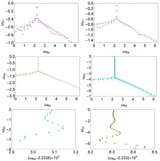
Figure 5. The spectral instability in the modified Pöschl–Teller effective potential Equation (6) triggered by a random perturbation Equation (12), where one assumes $V_0=b=5$ and for the deterministic perturbation $k=1$ with strength $ϵ=1\times {10}^{-3}$. Similar to Figure 4, for random perturbations of a given strength, two sets of results are presented in each panel. From left to right and top to bottom, we show the resulting QNM spectra for different perturbations using the magnitudes $\epsilon =1\times {10}^{-3}$ (empty red circles and empty blue squares), $1\times {10}^{-5}$ (empty blue squares and empty orange diamonds), $1\times {10}^{-10}$ (empty orange diamonds and empty gray triangles), $1\times {10}^{-30}$ (filled cyan circles and filled pink squares), a magnified view of the slightly modified low-lying modes of the last panel with identical $\epsilon =1\times {10}^{-30}$ (filled cyan circles and filled pink squares), $1\times {10}^{-50}$ (filled dark-yellow diamonds and filled pink squares). The numerical calculations are carried out using the matrix method.

In Figure 6, we perform a comparison between the QNM spectra presented in Figure 4 and Figure 5. Overall, one immediately identifies a strong resemblance between the two panels. By comparing the deviation of a given overtone of the spectrum triggered by random perturbations of different magnitudes, the spectral instability is more pronounced as the magnitude of the perturbation increases. However, while observing more closely, one might wonder whether the oscillating deviation observed in the bottom-right panel of Figure 5 might also appear in the case of random perturbations consisting of pure white noise. This is not the case, as demonstrated in Figure 7.

Figure 6. A summary of the changes in the QNM spectra shown in Figure 4 (left) and Figure 5 (right), where one enlists the following strengths of the random perturbations $\epsilon =1\times {10}^{-3}$, $1\times {10}^{-5}$, $1\times {10}^{-10}$, $1\times {10}^{-15}$, $1\times {10}^{-20}$, $1\times {10}^{-30}$, $1\times {10}^{-50}$.

Figure 7. A magnified view of the low-lying modes of the random perturbation Equation (10) with $\epsilon =1\times {10}^{-50}$ (similar to the panels shown in Figure 4), as a direct comparison with the bottom-right panel of Figure 5.

4. Sensitivity of Spectral Instability on the Localization of the Perturbation

Last but not least, we investigate the effect of localizing the perturbation. As shown in Refs. [42,55,64,69], the spectral instability becomes more severe as the perturbation moves toward spatial infinity. However, as pointed out in [43], to address this point more clearly, one must carefully consider perturbations that are physically relevant.

For this purpose, we consider the following localized perturbation of Gaussian shape in the tortoise coordinate

$$V_{\mathrm{pert}}^{\mathrm{loc}}={\displaystyle \frac{ϵ}{\sigma \sqrt{2\pi }}}{e}^{-{\displaystyle \frac{1}{2}}{\left({\displaystyle \frac{(r_{\ast }-r_c)}{\sigma }}\right)}^2},$$

(13)

with strength $ϵ$, centered at the coordinate $r_{\ast }=r_c$ with standard deviation $\sigma =1$. Specifically, the magnitude $ϵ$ is scaled so that $ϵ(r_c=r_0)={ϵ}_0$, where $r_0$ is the initial location of the perturbation. Here, we choose a particular scheme where $ϵ$ is inversely proportional to the squared distance

$$ϵ={ϵ}_0{\left({\displaystyle \frac{r_0}{r_c}}\right)}^2.$$

(14)

This is motivated to simulate a perturbation whose total energy roughly remains constant as its location moves away from the compact object.

The numerical results are presented in Figure 8. Owing to the scaling Equation (14), one observes that the spectral instability becomes less pronounced as the location of the perturbation moves away. Apparently, such a result is in agreement with physical intuition that a given perturbation in the potential should introduce less of an impact to the gravitational system when it is planted farther away from it. Meanwhile, it is in contrast to most existing studies, where an opposite effect has been observed in not only the high overtones [69] but also the fundamental mode [42,55,64]. The primary reason for this difference is that those studies considered a more straightforward setup in which the magnitude of the perturbation remains unchanged. Therefore, the present result indicates that the physical relevance of the perturbation plays a crucial role in such analyses. We note that in Figure 8, we take $V_0=1$ and $b=1$ to make the perturbation more pronounced. The numerical results indicate that the spectral instability becomes less evident as the perturbation moves away, even for such a choice. Nonetheless, owing to the direct impact of the fundamental mode on the time-domain waveforms, it is arguable that the observational implications are substantial.

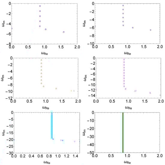
Figure 8. The spectral instability in the modified Pöschl–Teller effective potential Equation (6) triggered by a localized perturbation Equation (13) placed at different radial coordinates, where one assumes $V_0=b=1$, ${ϵ}_0=1\times {10}^{-10}$, $\sigma =1$, and $r_0=2$. For a given perturbation, two sets of results are presented in each panel. From left to right and top to bottom, we compare in pairs the resulting QNM spectra for different perturbations using different locations $r_c=5$ (empty red circles and empty blue squares), 7 (empty blue squares and empty orange diamonds), 10 (empty orange diamonds and empty gray triangles), 12 (empty gray triangles and empty magenta flipped triangles), 15 (empty magenta flipped triangles and filled cyan circles), 20 (filled cyan circles and filled dark-yellow squares). The numerical calculations are carried out using the matrix method.

5. Concluding Remarks

To summarize, we analyzed the spectral instability in the QNMs triggered by random and deterministic perturbations of the effective potential. We investigate the dependence on the magnitude, spatial scale, and localization of the perturbations and discuss the underlying physical interpretations. Small perturbations were observed to initially have a limited impact on the less damped black hole QNMs, and deviations typically oscillate around their unperturbed values, in agreement with a phenomenon first derived by Skakala and Visser in a more restrictive context. As either the frequency or the magnitude of the perturbations increases, in the higher-overtone region, the deviation propagates, amplifies, and eventually gives rise to spectral instability and, inclusively, bifurcation in the QNM spectrum. On the one hand, deterministic perturbations yield a modified but well-defined quasinormal spectrum. On the other hand, random perturbations lead to uncertainties in the resulting spectrum, while the primary trend of the spectral instability shows consistency. Additionally, the location of the perturbation was found to play a significant role in the resulting QNM spectrum. In contrast to most results in the literature, we show that the observed spectral instability as the localized perturbation moves away from the compact object might become suppressed once the underlying perturbation is revised to be physically appropriate. We conclude by pointing out substantial observational implications of the spectral instability and plan to continue to work on this pertinent topic.

References

- Abbott, B.P. [LIGO Scientific Collaboration and Virgo Collaboration]. Observation of Gravitational Waves from a Binary Black Hole Merger. Phys. Rev. Lett. 2016, 116, 061102. [Google Scholar] [CrossRef]
- Abbott, B.P. et al. [LIGO Scientific and Virgo Collaborations] Tests of general relativity with GW150914. Phys. Rev. Lett. 2016, 116, 221101, Erratum in Phys. Rev. Lett. 2018, 121, 129902.. [Google Scholar] [CrossRef]
- Abbott, B.P. et al. [LIGO Scientific Collaboration and Virgo Collaboration] GW151226: Observation of Gravitational Waves from a 22-Solar-Mass Binary Black Hole Coalescence. Phys. Rev. Lett. 2016, 116, 241103. [Google Scholar] [CrossRef]
- Abbott, B.P. et al. [LIGO Scientific Collaboration and Virgo Collaboration] GW170814: A Three-Detector Observation of Gravitational Waves from a Binary Black Hole Coalescence. Phys. Rev. Lett. 2017, 119, 141101. [Google Scholar] [CrossRef]
- Amaro-Seoane, P.; Audley, H.; Babak, S.; Baker, J.; Barausse, E.; Bender, P.; Berti, E.; Binetruy, P.; Born, M.; Bortoluzzi, D.; et al. Laser Interferometer Space Antenna. arXiv 2017. [Google Scholar] [CrossRef]
- Luo, J.; Chen, L.S.; Duan, H.-Z.; Gong, Y.-G.; Hu, S.; Ji, J.; Liu, Q.; Mei, J.; Milyukov, V.; Sazhin, M.; et al. TianQin: A space-borne gravitational wave detector. Class. Quant. Grav. 2016, 33, 035010. [Google Scholar] [CrossRef]
- Hu, W.R.; Wu, Y.L. The Taiji Program in Space for gravitational wave physics and the nature of gravity. Natl. Sci. Rev. 2017, 4, 685–686. [Google Scholar] [CrossRef]
- Shi, C.; Bao, J.; Wang, H.; Zhang, J.d.; Hu, Y.; Sesana, A.; Barausse, E.; Mei, J.; Luo, J. Science with the TianQin observatory: Preliminary results on testing the no-hair theorem with ringdown signals. Phys. Rev. D 2019, 100, 044036. [Google Scholar] [CrossRef]
- Nollert, H.P. TOPICAL REVIEW: Quasinormal modes: The characteristic ‘sound’ of black holes and neutron stars. Class. Quant. Grav. 1999, 16, R159–R216. [Google Scholar] [CrossRef]
- Berti, E.; Cardoso, V.; Starinets, A.O. Quasinormal modes of black holes and black branes. Class. Quant. Grav. 2009, 26, 163001. [Google Scholar] [CrossRef]
- Leaver, E.W. Spectral decomposition of the perturbation response of the Schwarzschild geometry. Phys. Rev. 1986, D34, 384–408. [Google Scholar] [CrossRef]
- Nollert, H.P.; Schmidt, B.G. Quasinormal modes of Schwarzschild black holes: Defined and calculated via Laplace transformation. Phys. Rev. 1992, D45, 2617. [Google Scholar] [CrossRef]
- Price, R.H. Nonspherical perturbations of relativistic gravitational collapse. 1. Scalar and gravitational perturbations. Phys. Rev. 1972, D5, 2419–2438. [Google Scholar] [CrossRef]
- Nollert, H.P. About the significance of quasinormal modes of black holes. Phys. Rev. 1996, D53, 4397–4402. [Google Scholar] [CrossRef]
- Nollert, H.P.; Price, R.H. Quantifying excitations of quasinormal mode systems. J. Math. Phys. 1999, 40, 980–1010. [Google Scholar] [CrossRef]
- Daghigh, R.G.; Green, M.D.; Morey, J.C. Significance of Black Hole Quasinormal Modes: A Closer Look. Phys. Rev. 2020, D101, 104009. [Google Scholar] [CrossRef]
- Qian, W.L.; Lin, K.; Shao, C.Y.; Wang, B.; Yue, R.H. Asymptotical quasinormal mode spectrum for piecewise approximate effective potential. Phys. Rev. 2021, D103, 024019. [Google Scholar] [CrossRef]
- Jaramillo, J.L.; Panosso Macedo, R.; Al Sheikh, L. Pseudospectrum and Black Hole Quasinormal Mode Instability. Phys. Rev. X 2021, 11, 031003. [Google Scholar] [CrossRef]
- Shen, S.F.; Li, G.R.; Daghigh, R.G.; Morey, J.C.; Green, M.D.; Qian, W.L.; Yue, R.H. Asymptotic quasinormal modes, echoes, and black hole spectral instability: A brief review. arXiv 2025. [Google Scholar] [CrossRef]
- Nollert, H.P. Quasinormal modes of Schwarzschild black holes: The determination of quasinormal frequencies with very large imaginary parts. Phys. Rev. 1993, D47, 5253–5258. [Google Scholar] [CrossRef]
- Motl, L. An Analytical computation of asymptotic Schwarzschild quasinormal frequencies. Adv. Theor. Math. Phys. 2003, 6, 1135–1162. [Google Scholar] [CrossRef]
- Dreyer, O.; Kelly, B.J.; Krishnan, B.; Finn, L.S.; Garrison, D.; Lopez-Aleman, R. Black hole spectroscopy: Testing general relativity through gravitational wave observations. Class. Quant. Grav. 2004, 21, 787–804. [Google Scholar] [CrossRef]
- Berti, E.; Cardoso, V.; Will, C.M. On gravitational-wave spectroscopy of massive black holes with the space interferometer LISA. Phys. Rev. 2006, D73, 064030. [Google Scholar] [CrossRef]
- Giesler, M.; Isi, M.; Scheel, M.A.; Teukolsky, S. Black Hole Ringdown: The Importance of Overtones. Phys. Rev. X 2019, 9, 041060. [Google Scholar] [CrossRef]
- Cabero, M.; Westerweck, J.; Capano, C.D.; Kumar, S.; Nielsen, A.B.; Krishnan, B. Black hole spectroscopy in the next decade. Phys. Rev. D 2020, 101, 064044. [Google Scholar] [CrossRef]
- Dhani, A. Importance of mirror modes in binary black hole ringdown waveform. Phys. Rev. D 2021, 103, 104048. [Google Scholar] [CrossRef]
- Liu, H.; Zhang, C.; Gong, Y.; Wang, B.; Wang, A. Exploring nonsingular black holes in gravitational perturbations. Phys. Rev. 2020, D102, 124011. [Google Scholar] [CrossRef]
- Pani, P. Advanced Methods in Black-Hole Perturbation Theory. Int. J. Mod. Phys. 2013, A28, 1340018. [Google Scholar] [CrossRef]
- Berti, E.; Cardoso, V.; Carullo, G.; Abedi, J.; Afshordi, N.; Albanesi, S.; Baibhav, V.; Bhagwat, S.; Blázquez-Salcedo, J.; Bonga, B.; et al. Black hole spectroscopy: From theory to experiment. arXiv 2025. [Google Scholar] [CrossRef]
- Visser, M. Dirty black holes: Thermodynamics and horizon structure. Phys. Rev. 1992, D46, 2445–2451. [Google Scholar] [CrossRef]
- Leung, P.T.; Liu, Y.T.; Suen, W.M.; Tam, C.Y.; Young, K. Quasinormal modes of dirty black holes. Phys. Rev. Lett. 1997, 78, 2894–2897. [Google Scholar] [CrossRef]
- Leung, P.T.; Liu, Y.T.; Suen, W.M.; Tam, C.Y.; Young, K. Perturbative approach to the quasinormal modes of dirty black holes. Phys. Rev. 1999, D59, 044034. [Google Scholar] [CrossRef]
- Barausse, E.; Cardoso, V.; Pani, P. Can environmental effects spoil precision gravitational-wave astrophysics? Phys. Rev. 2014, D89, 104059. [Google Scholar] [CrossRef]
- Cardoso, V.; Franzin, E.; Pani, P. Is the gravitational-wave ringdown a probe of the event horizon? Phys. Rev. Lett. 2016, 116, 171101, Erratum in Phys. Rev. Lett. 2016, 117, 089902.. [Google Scholar] [CrossRef]
- Cardoso, V.; Pani, P. Testing the nature of dark compact objects: A status report. Living Rev. Rel. 2019, 22, 4. [Google Scholar] [CrossRef]
- Mark, Z.; Zimmerman, A.; Du, S.M.; Chen, Y. A recipe for echoes from exotic compact objects. Phys. Rev. 2017, D96, 084002. [Google Scholar] [CrossRef]
- Damour, T.; Solodukhin, S.N. Wormholes as Black Hole Foils. Phys. Rev. 2007, D76, 024016. [Google Scholar] [CrossRef]
- Bueno, P.; Cano, P.A.; Goelen, F.; Hertog, T.; Vercnocke, B. Echoes of Kerr-like wormholes. Phys. Rev. 2018, D97, 024040. [Google Scholar] [CrossRef]
- Gasperin, E.; Jaramillo, J.L. Energy scales and black hole pseudospectra: The structural role of the scalar product. Class. Quant. Grav. 2022, 39, 115010. [Google Scholar] [CrossRef]
- Jaramillo, J.L.; Panosso Macedo, R.; Sheikh, L.A. Gravitational Wave Signatures of Black Hole Quasinormal Mode Instability. Phys. Rev. Lett. 2022, 128, 211102. [Google Scholar] [CrossRef]
- Destounis, K.; Macedo, R.P.; Berti, E.; Cardoso, V.; Jaramillo, J.L. Pseudospectrum of Reissner-Nordström black holes: Quasinormal mode instability and universality. Phys. Rev. D 2021, 104, 084091. [Google Scholar] [CrossRef]
- Cheung, M.H.Y.; Destounis, K.; Macedo, R.P.; Berti, E.; Cardoso, V. Destabilizing the Fundamental Mode of Black Holes: The Elephant and the Flea. Phys. Rev. Lett. 2022, 128, 111103. [Google Scholar] [CrossRef]
- Berti, E.; Cardoso, V.; Cheung, M.H.Y.; Di Filippo, F.; Duque, F.; Martens, P.; Mukohyama, S. Stability of the fundamental quasinormal mode in time-domain observations against small perturbations. Phys. Rev. D 2022, 106, 084011. [Google Scholar] [CrossRef]
- Kyutoku, K.; Motohashi, H.; Tanaka, T. Quasinormal modes of Schwarzschild black holes on the real axis. Phys. Rev. D 2023, 107, 044012. [Google Scholar] [CrossRef]
- Jaramillo, J.L. Pseudospectrum and binary black hole merger transients. Class. Quant. Grav. 2022, 39, 217002. [Google Scholar] [CrossRef]
- Konoplya, R.A.; Zinhailo, A.F.; Kunz, J.; Stuchlik, Z.; Zhidenko, A. Quasinormal ringing of regular black holes in asymptotically safe gravity: The importance of overtones. J. Cosmol. Astropart. Phys. 2022, 10, 091. [Google Scholar] [CrossRef]
- Boyanov, V.; Destounis, K.; Panosso Macedo, R.; Cardoso, V.; Jaramillo, J.L. Pseudospectrum of horizonless compact objects: A bootstrap instability mechanism. Phys. Rev. D 2023, 107, 064012. [Google Scholar] [CrossRef]
- Liu, H.; Qian, W.L.; Liu, Y.; Wu, J.P.; Wang, B.; Yue, R.H. Alternative mechanism for black hole echoes. Phys. Rev. 2021, D104, 044012. [Google Scholar] [CrossRef]
- Hui, L.; Kabat, D.; Wong, S.S.C. Quasinormal modes, echoes and the causal structure of the Green’s function. J. Cosmol. Astropart. Phys. 2019, 12, 020. [Google Scholar] [CrossRef]
- Yang, H.; Zhang, J. Spectral stability of near-extremal spacetimes. Phys. Rev. D 2023, 107, 064045. [Google Scholar] [CrossRef]
- Courty, A.; Destounis, K.; Pani, P. Spectral instability of quasinormal modes and strong cosmic censorship. Phys. Rev. D 2023, 108, 104027. [Google Scholar] [CrossRef]
- Sarkar, S.; Rahman, M.; Chakraborty, S. Perturbing the perturbed: Stability of quasinormal modes in presence of a positive cosmological constant. Phys. Rev. D 2023, 108, 104002. [Google Scholar] [CrossRef]
- Cardoso, V.; Kastha, S.; Panosso Macedo, R. Physical significance of the black hole quasinormal mode spectra instability. Phys. Rev. D 2024, 110, 024016. [Google Scholar] [CrossRef]
- Qian, W.L.; Li, G.R.; Daghigh, R.G.; Randow, S.; Yue, R.H. Universality of instability in the fundamental quasinormal modes of black holes. Phys. Rev. D 2025, 111, 024047. [Google Scholar] [CrossRef]
- Yang, Y.; Mai, Z.F.; Yang, R.Q.; Shao, L.; Berti, E. Spectral instability of black holes: Relating the frequency domain to the time domain. Phys. Rev. D 2024, 110, 084018. [Google Scholar] [CrossRef]
- Shen, S.F.; Lin, K.; Zhu, T.; Yan, Y.P.; Shao, C.G.; Qian, W.L. Two distinct types of echoes in compact objects. Phys. Rev. D 2024, 110, 084022. [Google Scholar] [CrossRef]
- Rosato, R.F.; Destounis, K.; Pani, P. Ringdown stability: Graybody factors as stable gravitational-wave observables. Phys. Rev. D 2024, 110, L121501. [Google Scholar] [CrossRef]
- Oshita, N.; Takahashi, K.; Mukohyama, S. Stability and instability of the black hole greybody factors and ringdowns against a small-bump correction. Phys. Rev. D 2024, 110, 084070. [Google Scholar] [CrossRef]
- Rosato, R.F.; Biswas, S.; Chakraborty, S.; Pani, P. Greybody factors, reflectionless scattering modes, and echoes of ultracompact horizonless objects. Phys. Rev. D 2025, 111, 084051. [Google Scholar] [CrossRef]
- Daghigh, R.G.; Li, G.R.; Qian, W.L.; Randow, S.J. Evolution of black hole echo modes and the causality dilemma. Phys. Rev. D 2025, 111, 124021. [Google Scholar] [CrossRef]
- Li, G.R.; Qian, W.L.; Pan, Q.; Daghigh, R.G.; Morey, J.C.; Yue, R.H. Regge poles, greybody factors, and absorption cross sections for black hole metrics with discontinuity. Phys. Rev. D 2025, 112, 064071. [Google Scholar] [CrossRef]
- Mai, Z.F.; Yang, R.Q. Butterfly in Spacetime: Inherent Instabilities in Stable Black Holes. arXiv 2025. [Google Scholar] [CrossRef]
- Wu, L.B.; Xie, L.; Zhou, Y.S.; Guo, Z.K.; Cai, R.G. Waveform stability for the piecewise step approximation of Regge-Wheeler potential. arXiv 2025. [Google Scholar] [CrossRef]
- Ianniccari, A.; Iovino, A.J.; Kehagias, A.; Pani, P.; Perna, G.; Perrone, D.; Riotto, A. Deciphering the Instability of the Black Hole Ringdown Quasinormal Spectrum. Phys. Rev. Lett. 2024, 133, 211401. [Google Scholar] [CrossRef]
- Motohashi, H. Resonant Excitation of Quasinormal Modes of Black Holes. Phys. Rev. Lett. 2025, 134, 141401. [Google Scholar] [CrossRef] [PubMed]
- Lin, K.; Qian, W.L. A Matrix Method for Quasinormal Modes: Schwarzschild Black Holes in Asymptotically Flat and (Anti-) de Sitter Spacetimes. Class. Quant. Grav. 2017, 34, 095004. [Google Scholar] [CrossRef]
- Ferrari, V.; Mashhoon, B. New approach to the quasinormal modes of a black hole. Phys. Rev. 1984, D30, 295–304. [Google Scholar] [CrossRef]
- Zenginoğlu, A. A geometric framework for black hole perturbations. Phys. Rev. 2011, D83, 127502. [Google Scholar] [CrossRef]
- Li, G.R.; Qian, W.L.; Daghigh, R.G. Bifurcation and spectral instability of asymptotic quasinormal modes in the modified Pöschl-Teller effective potential. Phys. Rev. D 2024, 110, 064076. [Google Scholar] [CrossRef]
- Shen, S.F.; Qian, W.L.; Guo, H.; Zhang, S.J.; Li, J. An implementation of the matrix method using the Chebyshev grid. Prog. Theor. Exp. Phys. 2023, 2023, 093E01. [Google Scholar] [CrossRef]
- Skakala, J.; Visser, M. Semi-analytic results for quasi-normal frequencies. J. High Energy Phys. 2010, 8, 61. [Google Scholar] [CrossRef]
- Skakala, J.; Visser, M. Highly-damped quasi-normal frequencies for piecewise Eckart potentials. Phys. Rev. 2010, D81, 125023. [Google Scholar] [CrossRef]
- Chandrasekhar, S. On algebraically special perturbations of black holes. Proc. Roy. Soc. Lond. A 1984, 392, 1–13. [Google Scholar] [CrossRef]
Disclaimer/Publisher’s Note: The statements, opinions and data contained in all publications are solely those of the individual author(s) and contributor(s) and not of MDPI and/or the editor(s). MDPI and/or the editor(s) disclaim responsibility for any injury to people or property resulting from any ideas, methods, instructions or products referred to in the content. |
© 2025 by the authors. Licensee MDPI, Basel, Switzerland. This article is an open access article distributed under the terms and conditions of the Creative Commons Attribution (CC BY) license.