Article

Day-Time Seeing Changes at the Huairou Solar Observing Station Site

by
Artem Y. Shikhovtsev
Institute of Solar-Terrestrial Physics, The Siberian Branch of the Russian Academy of Sciences, Irkutsk 664033, Russia
Universe 2026, 12(1), 11; https://doi.org/10.3390/universe12010011 (registering DOI)
Submission received: 8 December 2025 / Revised: 24 December 2025 / Accepted: 27 December 2025 / Published: 1 January 2026

Abstract

In this paper, a simple method of estimating reference optical turbulence profiles at the Huairou Solar Observing Station (HSOS) from a large meteorological dataset is used. These reference profiles can be used in simulations of atmospheric variability above the station and the impact of climate change on image quality. By analyzing the statistics of measured optical turbulence and using the ERA-5 reanalysis data, vertical distributions of optical turbulence above HSOS were obtained for different time periods (1940–1969, 1970–1999, 1989–2010, 2000–2025). It has been shown that the intensity of optical turbulence in the surface layer has been decreasing in recent decades, while the intensity in the upper troposphere has a tendency to increase. Trends are also assessed in total cloud cover and atmospheric boundary layer height at the HSOS site. Observed changes are associated with global warming.

1. Introduction

Climate change has a strong impact on atmospheric properties relevant for observational astronomy. However, studies considering the impact of climate change on astronomical observations started to emerge only recently [1]. For example, Cantalloube et al. conducted a study for Cerro Paranal on the impact of climate change on meteorological characteristics, including synoptic and optical turbulence scales [2]. Seidel J. et al. conducted an analysis of the surface-level air temperature, water vapour density, and astronomical seeing at the European Southern Observatory telescope sites in northern Chile [3]. Long-period changes in astroclimatic characteristics (including seeing) have been studied for a number of sites in Eurasia [4,5,6]. At the Lenghu site, Yong Zhao et al. conducted a comprehensive analysis of the long-term variations in meteorological variables [7]. It was shown that the average values of precipitable water vapor, wind speed on 200 hPa, and total cloud cover from 1990 to 2023 were stable.
Image quality of ground-based astronomical telescopes is largely depends on atmospheric optical turbulence strength along the line of sight (ALS) [8]. In particular, the intensity of air refractive index turbulent fluctuations ALS determines the resolving power of the telescope. For a long exposure, the key value is the full width at half maximum (FWHM) of the point spread function. FWHM is often used to quantify the achieved image resolution. In a turbulent atmosphere, the angular size of the image (seeing) may be estimated using the following formula [9]:
β = 0.98 λ r 0 = 0.98 λ ( 0.423 ( 2 π λ ) 2 s e c α S 0 H C n 2 ( Z ) d Z ) 3 / 5 ,
where λ is the light wavelength, α S is the zenith angle of the observed light source, C n 2 is the structural characteristic of the air refractive index fluctuations, Z is the height of the turbulent layer above the ground, r 0 is the Fried parameter. r 0 is the key characteristic of atmospheric optical turbulence, defined as the diameter of a circular area over which the rms wavefront aberration is equal to 1 radian. In fact, this value determines the linear scales of atmospheric coherent optical inhomogeneities: when the wavefront passes through these inhomogeneities, its surface remains close to the plane. As these scales increase, the resolving power of telescopes improves and the size of various details on the solar surface decreases. It should be noted that the above formula is valid for describing daytime and nighttime turbulence. The main limitation of its application is that the turbulence must obey the Kolmogorov model. Namely, the spectral density of turbulent fluctuations in the air refractive index must be proportional to the wavenumber to the power of −5/3.
Characteristics of astronomical image quality and atmospheric optical turbulence are of great interest. In addition to assessing spatiotemporal variations in optical turbulence for characterizing an astronomical site [10,11], developing machine learning models that predict image quality [12,13,14,15], it is important to evaluate the impact of climate change on astronomical observations. Of particular interest are short tipping periods when the climate system undergoes significant alteration. During these moments, atmospheric characteristics can exceed their threshold values, leading to sharp variations in climate system parameters. According to the World Meteorological Organization, 2024 was the warmest year on record; the past ten years demonstrate an extraordinary streak of record-breaking temperatures.
It is no secret that global warming observed in the lower atmosphere is changing many of the atmosphere’s thermodynamic properties [16]. Conditions for astronomical observations are also changing. In this regard, the study was aimed at assessing long-period changes in atmospheric characteristics relevant for astronomical observations. The site of the Huairou Solar Observing Station (HSOS) located in China was chosen as an example. This station, an instrument of the National Astronomical Observatories of the Chinese Academy of Sciences, is located on the northern shore of the Huairou Reservoir, 60 km north of central Beijing (40°20′ N 116°30′ E). The proximity of the water reservoir makes the atmospheric conditions at this station similar to those of the Large Solar Vacuum Telescope (LSVT (51°51′ N 104°53′ E)) (LSVT). Meteorological fields above these sites are under the stabilizing influence of a large water body. Also, both sites have low elevations above sea level.
The specific tasks of the study are as follows:
(1)
Identification of features in the vertical structure of optical turbulence above the station. Determination of the changes in image quality characteristics over the past decades;
(2)
Estimation of long-period changes in another important astroclimatic quantity, total cloud cover (TCC), which determines the amount of observing time at the station.
Estimates of long-period changes in turbulence and cloudiness can be useful in searching for the consequences of climate change impacts on parameters relevant to astronomical observations. In this paper, an attempt is made to find some features in long-term changes in atmospheric characteristics that would fit into the modern patterns of global climate change. In particular, the hypothesis that changes in the properties of the atmospheric optical screen that forms in the upper troposphere/lower stratosphere have a significant impact on climate is considered [17]. Turbulence at these altitudes determines the orientation of particles (which structure clouds). If turbulence decreases, one can expect these particles to align, forming a thin atmospheric layer with increased reflectivity. As turbulence increases, particle mixing improves, and the modulating properties of the optical screen decrease. This leads to a significant reduction in scattered light and contributes somewhat to global temperature increases on the Earth. Unfortunately, experiments capable of confirming this hypothesis have not yet been conducted. This paper attempts to obtain evidence for the plausibility of this assumption by analyzing meteorological data from the reanalysis.

2. Materials and Methods

For the determination of the atmospheric characteristics, both ERA-5 reanalysis data and accumulated observations of solar image quality characteristics were used [18,19]. The ERA-5 database contains hourly meteorological characteristics at different altitudes in the atmosphere and is the result of assimilation of various measurement data. Accumulated experience shows that reanalysis can be used to estimate atmospheric conditions above astronomical observatories with acceptable accuracy [20,21]. Individual results also indicate the validity of using reanalysis to describe the atmosphere, including over and near water reservoirs. For example, Liu et al. demonstrated that ERA-5 data agree well with measurements over the South China Sea [22].
In this study, temporal trends in the TCC and BLH were obtained by processing hourly values from 1940 to 2025. In order to simulate the vertical profiles of C n 2 , a classical approach based on calculating vertical gradients of meteorological characteristics was applied [23], supplemented by two calibration stages.
In particular, the calculation of C n 2 is based on classical formulas:
C n 2 ( z ) = A m α L 0 ( z ) 4 / 3 M 2 ( z ) .
In this expression, the intensity of optical (small-scale) turbulence ( C n 2 ) is related to the mean vertical gradient of the air refractive index M ( z ) and the outer scale of turbulence L 0 . α is a numerical constant, which is equal to 2.8, A m is the coefficient determined by comparing the measured and calculated values of β . The parameter M ( z ) can be estimated using the following:
M ( z ) = 79 · 10 6 P ( z ) T ( z ) l n θ ( z ) z ,
where P is the atmospheric pressure and T is the air temperature. θ is the potential air temperature:
θ ( z ) = T ( z ) 1000 P ( z ) 0.286 .
The key parameter is the outer scale of atmospheric turbulence L 0 . In general, vertical changes in the outer scale L 0 can be parameterized through the vertical gradients of the horizontal component of the wind velocity:
L 0 ( z ) 4 / 3 = 0 . 1 4 / 3 · 10 A L + B d V · S ( z ) , troposphere 0 . 1 4 / 3 · 10 A L 2 + B d V 2 · S ( z ) , stratosphere ,
where
S ( z ) = u ( z ) z 2 + v ( z ) z 2 0.5 ,
u and v are the horizontal components of wind velocity, A L , B d V , A L 2 and B d V 2 are parameterization coefficients.
The approach based on the use of meteorological parameters is appropriate because the observed turbulence is often associated with large-scale flow disturbances, vertical wind shears, airflow deformation and divergence [24].
The first stage of calibration involves selecting optimal parameterization coefficients. While it is acceptable to use standard values of the coefficients within the stratosphere, where the intensity of optical turbulence is low, the coefficients in the troposphere and its lower part must be refined. To solve this issue, the accumulated archive of differential motion of solar subimages recorded by the Large Solar Vacuum Telescope and data from mast acoustic measurements in the surface layer of the atmosphere were used.
The refinement of the parameterization coefficients is based on the following:
(i)
Processing of solar photosphere hartmannograms recorded with frequencies from 80 to 300 Hz. In fact, using a large set of sub-images, differential displacements of their gravity centers are determined. The dispersion of differential displacements may be calculated using the following:
σ α 2 = K λ 2 r 0 5 / 3 D 1 / 3 ,
where D is the telescope diameter (D = 600 mm). The coefficient K used in Formula (7) depends on the ratio of the distance between the centers of the subapertures S d and the subaperture diameter d s , as well as the direction of image motion and the type of wavefront slope. Longitudinal and transverse coefficients are as follows:
K l = 0.34 1 0.57 S d d s 1 / 3 0.04 S d d s 7 / 3 ,
K t = 0.34 1 0.855 S d d s 1 / 3 + 0.03 S d d s 7 / 3 .
Large Solar Vacuum Telescope, adaptive optics system, and the example of a sunspot Hartmannogram at the second focus of the Large Solar Vacuum Telescope are shown in Figure 1. Table 1 shows parameters of LSVT and optical setup.
(ii)
The Fried parameter estimated by integration of the modeled C n 2 along the height must be close to its measured value (from the differential motion of images). In othe ptical turbulence profile, the ground value of C n 2 is set based on the processing of sonic measurements. The sonic measurements make it possible to refine the parameterization coefficients used in calculating the outer scale L 0 .
By processing data of differential motion of solar subimages, as well as data from sonic measurements of surface turbulence, we refined the parameterization coefficients. Parameterization coefficients for different values of the Fried parameter are given in Table 2. Medians of the Fried parameter for the LSVT site are listed in Table 3.
In the second stage of calibration, the values of the structural characteristic C n 2 were calibrated using Fried parameter values found from solar image processing (at HSOS). The results of the processing of monochrome solar images at the site of HSOS are presented in the paper [19].

3. Astroclimatic Characteristics at the Site of Huairou Solar Observing Station

3.1. Vertical Distributions of Optical Turbulence at the Site of Huairou Solar Observing Station

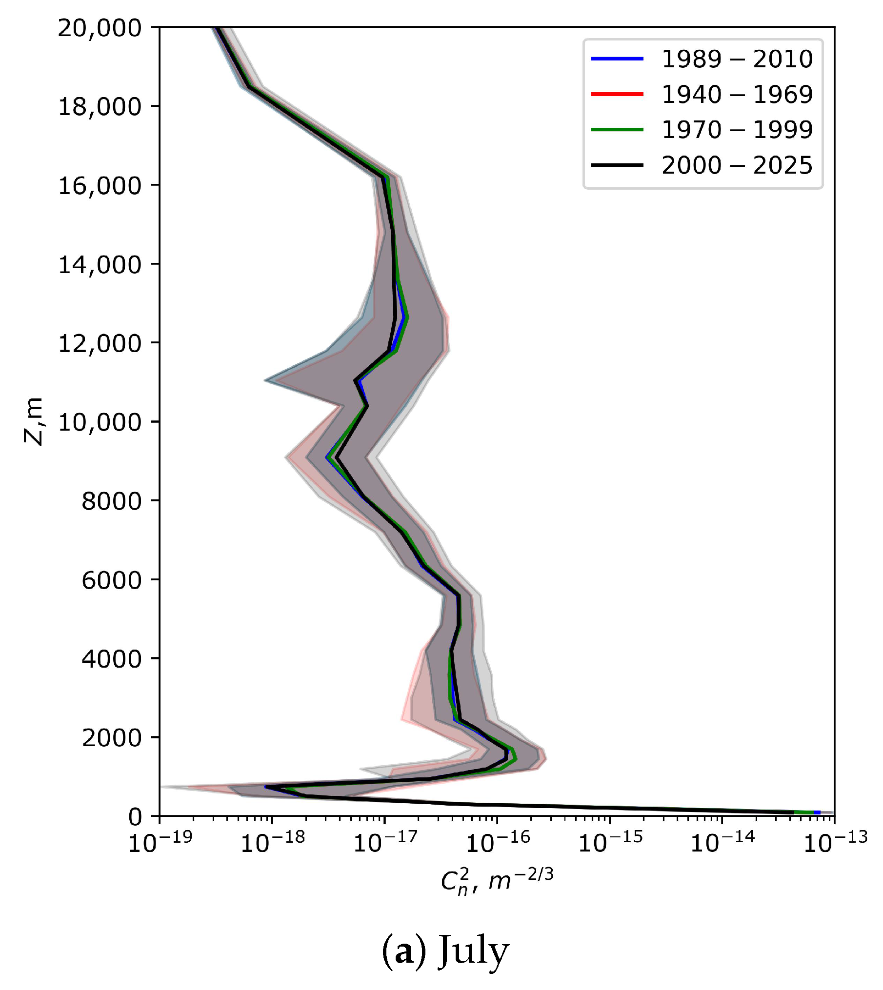
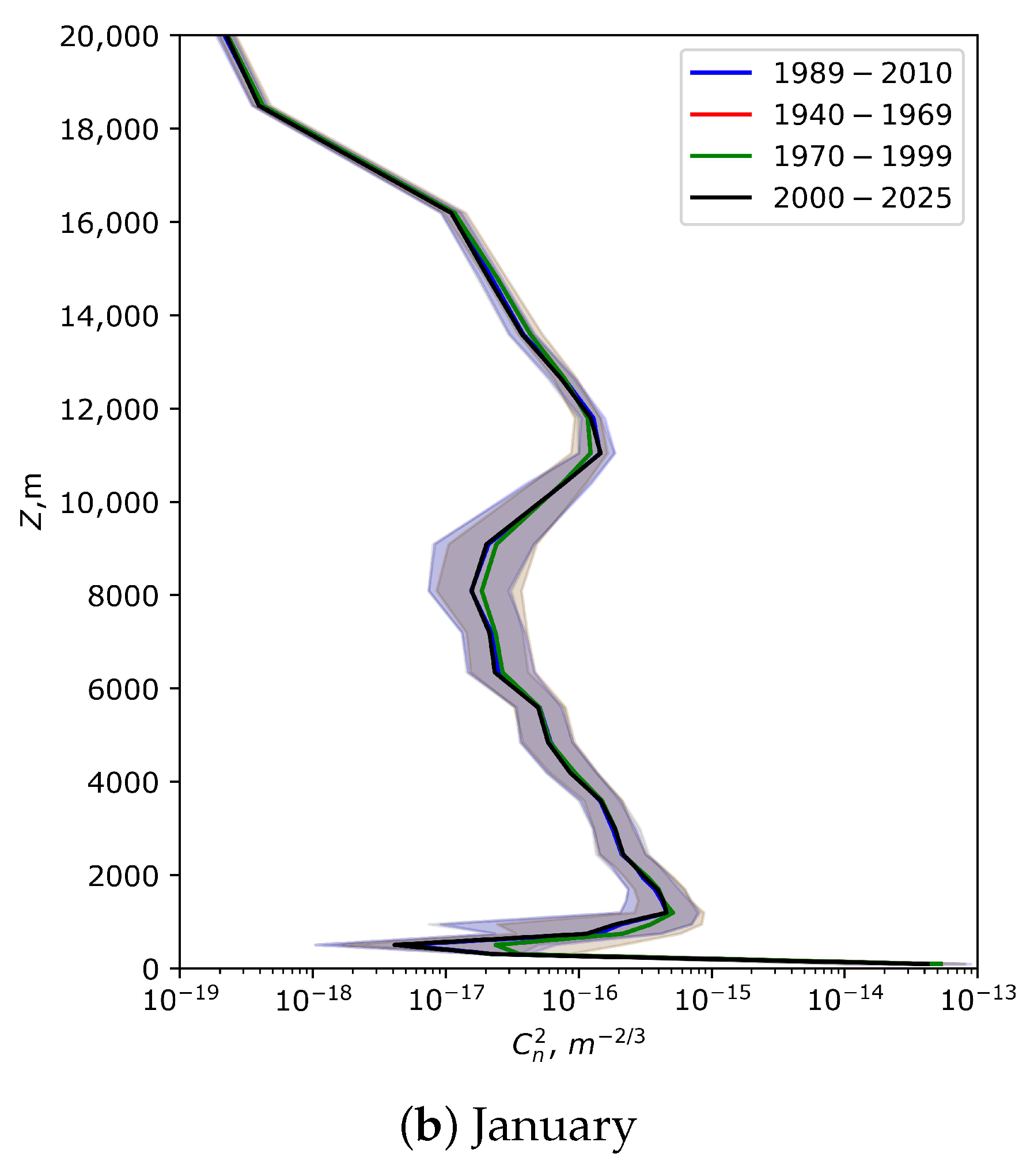
Using the ERA-5 reanalysis data and the above-mentioned approach based on meteorological characteristics, the vertical profiles of optical turbulence strength C n 2 at the HSOS site were obtained. Simulated daytime vertical profiles of optical turbulence strength C n 2 at the Huairou Solar Observing Station for different time periods are shown in Figure 2. Days with TCC > 0.5 were excluded.
Taking into account that the period that corresponds to the statistical ensemble of atmospheric states and the concept of climate is about 30 years, the vertical profiles C n 2 were calculated for the following time ranges: 1940–1969, 1970–1999, 2000–2025. The period from 1989 to 2010 was used as a reference. This choice is due to the fact that for this period, there are results of statistical processing of solar photosphere monochromatic images collected by the Solar Magnetic Field Telescope at the HSOS.
Analysis of the vertical profiles reveals nonlinear changes in turbulence strength in terms of the structural characteristics of the air refractive index fluctuations. Significant turbulent fluctuations are observed in the upper layer, at heights of 11,000–16,000 m, and also near the underlying surface—within the atmospheric boundary layer. This behavior of vertical changes in C n 2 is close to previously obtained results for a number of other observatories [25,26,27,28].
The medians, first and third quartile values of the Fried parameter are shown in Table 4 (January) and Table 5 (July). Analysis of Figure 2 shows that the vertical profiles C n 2 averaged over different long-term periods differ little from each other. These small differences are confirmed by the values of the Fried parameter, the value of which is inversely proportional to the total optical turbulence intensity along the height. This is an expected result since the structure of (optical) turbulence is largely random.
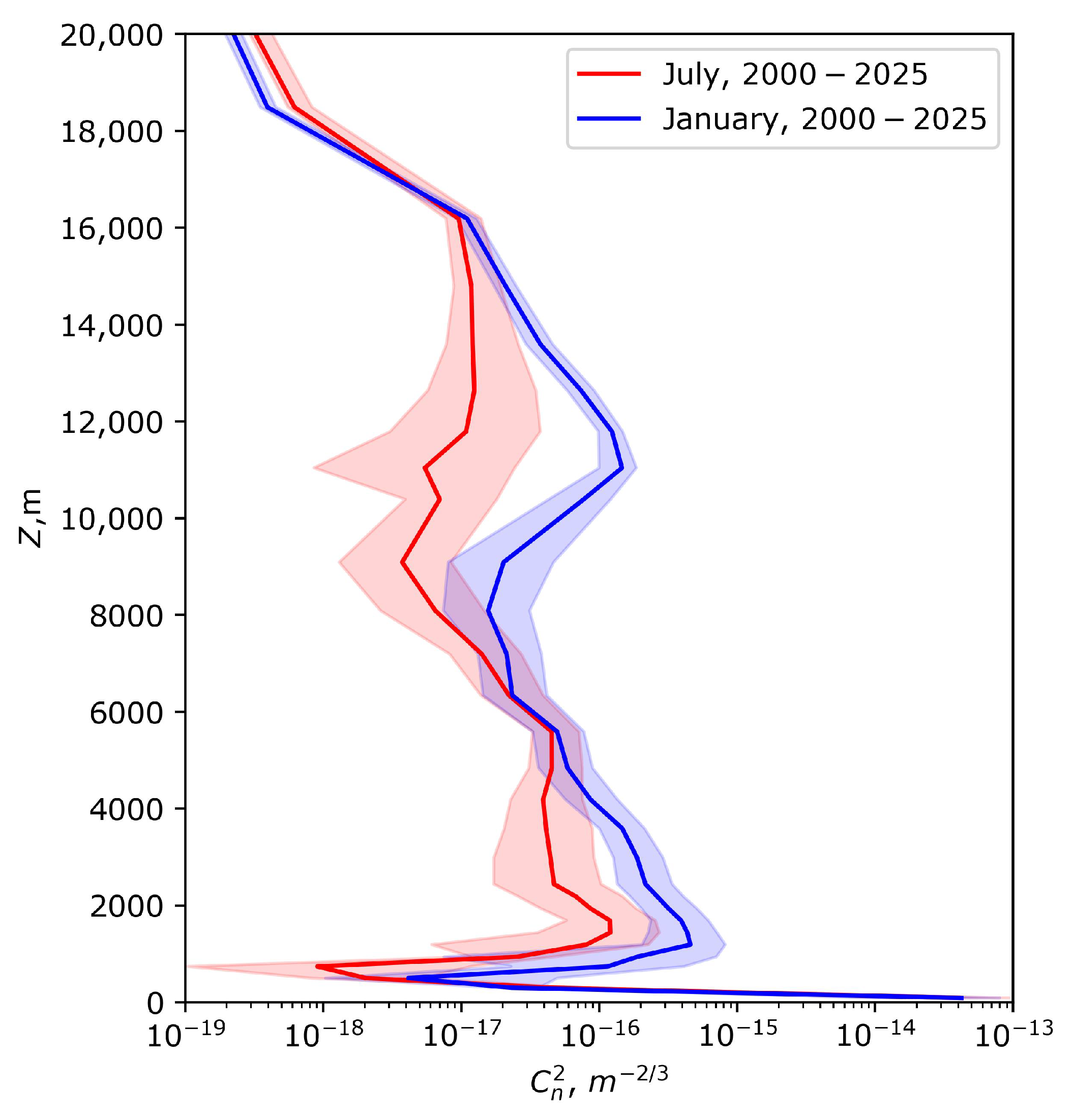
Vertical profiles of optical turbulence have the highest differences between winter and summer. Figure 3 shows simulated day-time vertical profiles of optical turbulence strength C n 2 at the Huairou Solar Observing Station in July and January for 2000–2025. The seasonal variation (peak-to-valley) of simulated total values r 0 is ∼12%.
Interesting questions include what quantitative estimations of the long-term changes in the optical turbulence strength are. In order to answer this question, the following characteristic was assessed:
F d = C n 2 ( z , 2000 2025 ) C n 2 ( z , 1940 1969 ) C n 2 ( z , 1940 1969 ) ,
where the averaging periods are shown in brackets.
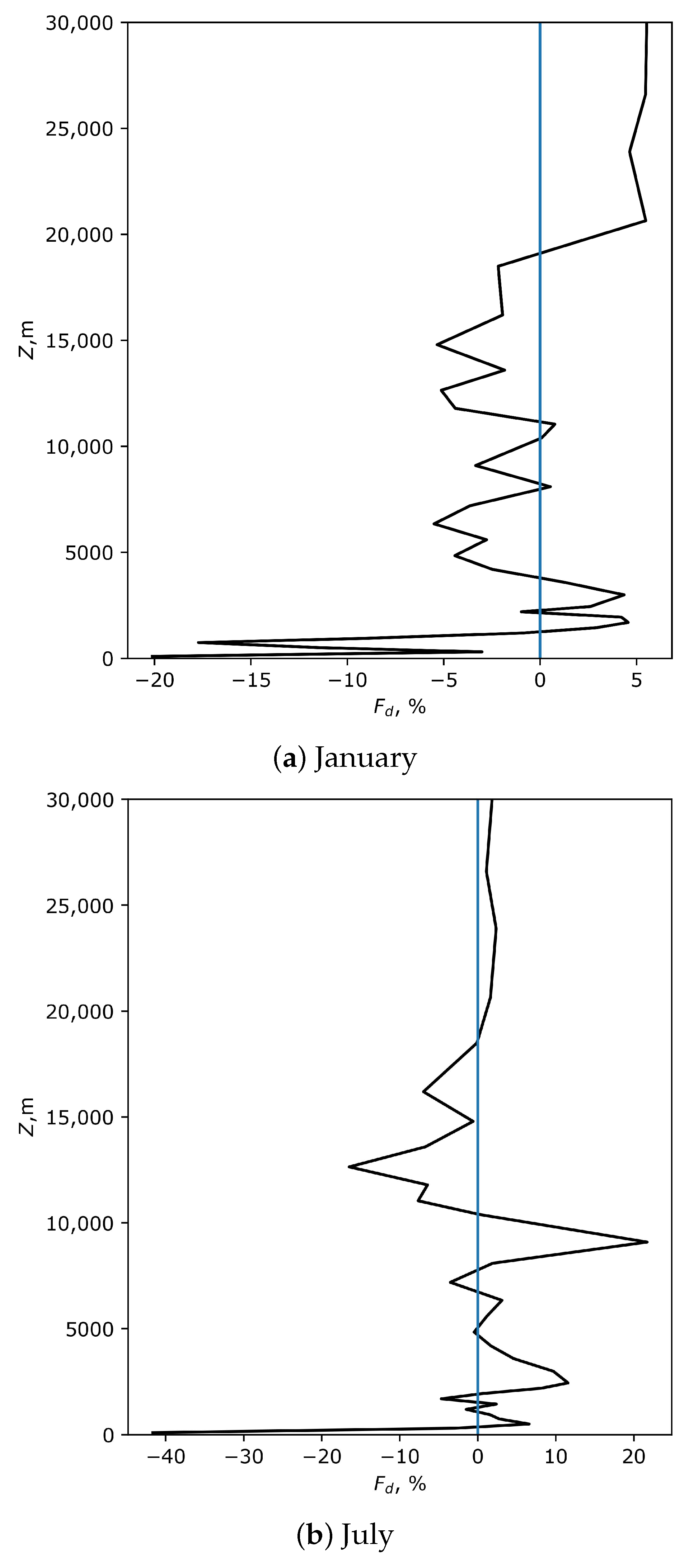
Day-time vertical distributions of F d at the Huairou are shown in Figure 4. F d values reflect the relative changes in the optical turbulence strength of atmospheric layers averaged over 1940–1969 and 2000–2025.
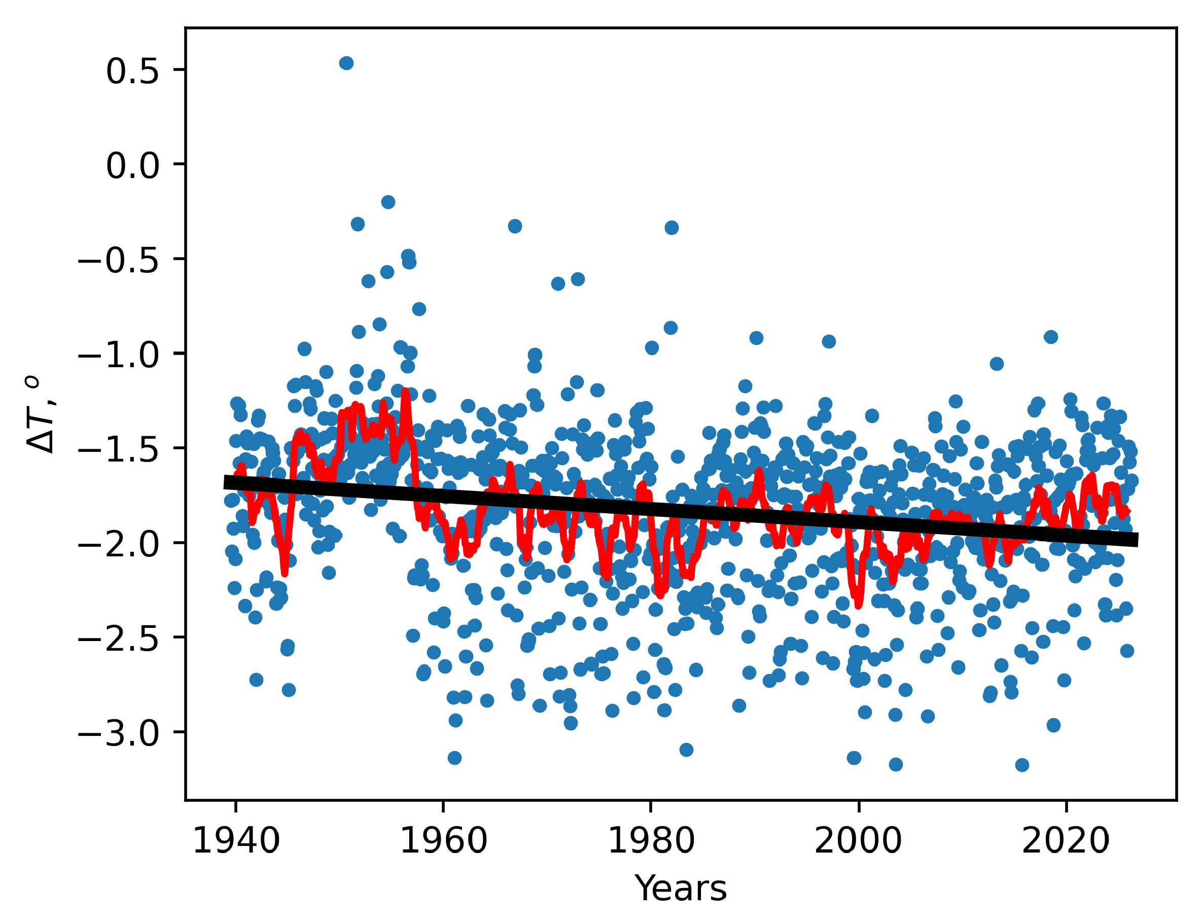
Optical turbulence relative strength variation ( F d ) occurs primarily in the lower atmosphere, within the atmospheric boundary layer, which most affects the seasonal trend of the total seeing. When comparing periods, 1940–1969 and 2000–2025, the decrease in surface turbulence intensity in January reaches 20% (in terms of C n 2 ). In July, this decrease is 40%. This circumstance is likely related to global warming, which has led to a significant reduction in large-scale horizontal temperature contrast (Equator-Pole). Daytime variations of the meridional gradient of air temperature at a height of 2 m Δ T at the HSO are shown in Figure 5. Calculations of Δ T were performed using ERA-5 monthly averaged data on single levels from 1940 to the present:
Δ T = t 2 m ( 40 . 5 N ) t 2 m ( 40 . 25 N ) ,
where t 2 m is the air temperature at 2 m. Latitudes are given in the brackets.
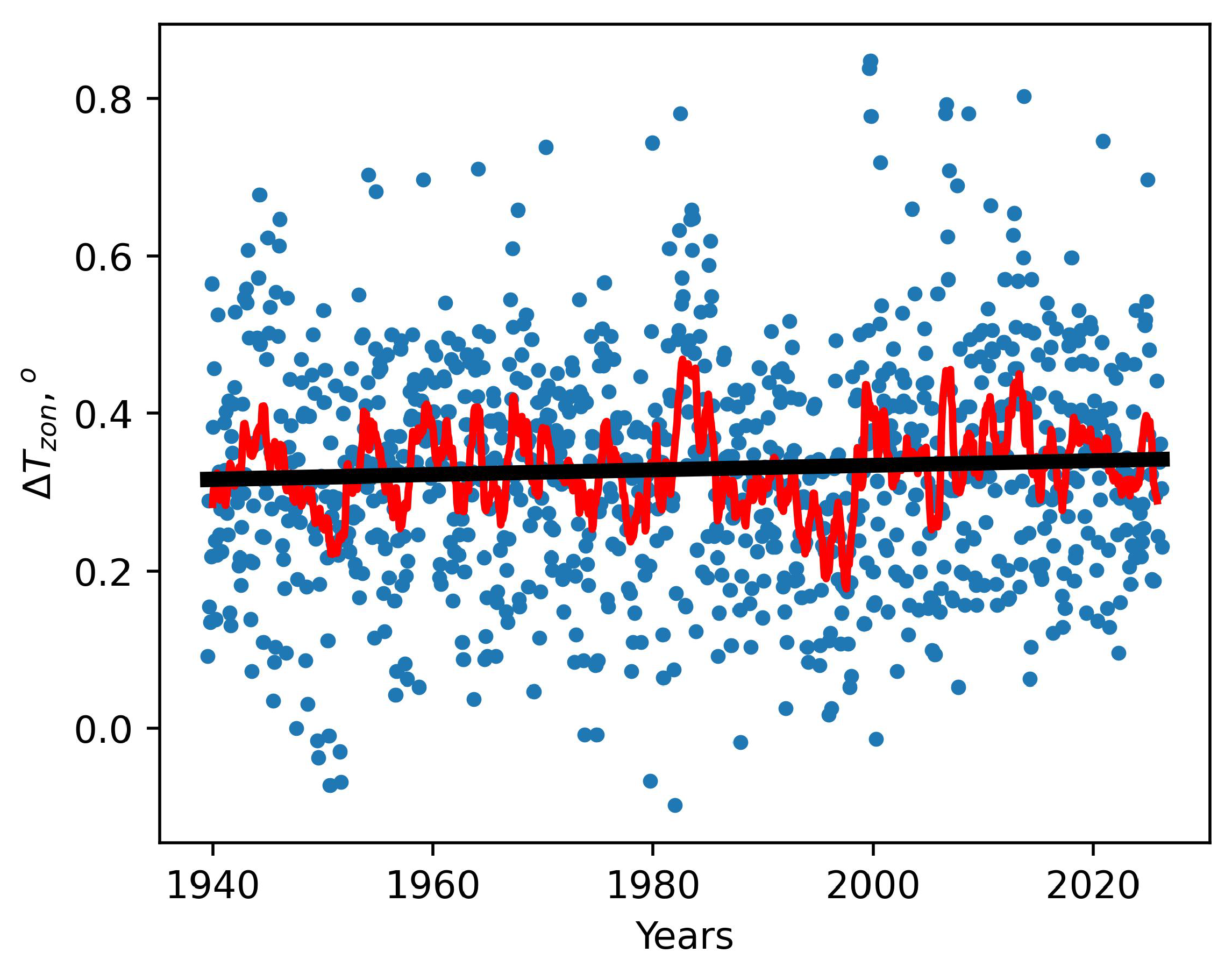
Analysis of Figure 5 shows that, in average, there is a tendency towards a decrease in the meridional air temperature gradient. An average trend in Δ T a Δ T = −0.035° per decade (∼0.30° per 85 yr., t = −6.49, p > | t | = 0.0). The zonal gradient Δ T z o n = t 2 m ( 116 . 75 E ) t 2 m ( 116 . 50 E ) has not changed (Figure 6).
During the winter period, a significant increase in stratospheric turbulence is observed. These variations are particularly important because they can alter the conditions for the evolution of atmospheric aerosol content.
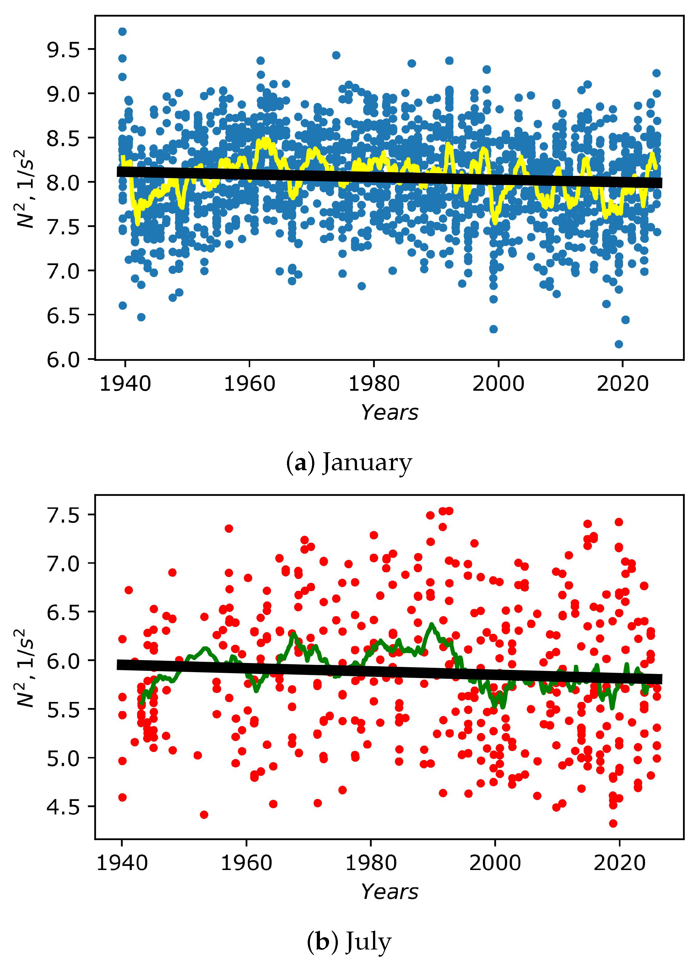
Evolution of moderate and strong clear-air turbulence, especially in regions influenced by the upper-level jet streams, is of great interest. For a deeper understanding of the conditions under which turbulence forms, the Brunt–Vaisala frequency N, a metric that measures the resistance of air parcels to vertical displacement [29] was estimated at HSOS. Values of N averaged within the atmospheric layer 100–250 hPa at HSOS are shown in Figure 7.
Negative trends in N 2 at these heights are observed. The calculation shows decreasing trends −0.015 per decade in January (t = −3.42, p > | t | = 0.01) and −0.017 per decade in July (t = −1.29, p > | t | = 0.20), respectively. These results may indicate the formation of favorable conditions for the development of turbulence in January (in the winter period). In my opinion, the increase in wind speed and turbulence in the upper atmosphere can lead to changes in the properties of the optical screen. In particular, as the velocity increases, the amount of aerosol and the level of scattered light can decrease.

3.2. Long-Period Changes in Daytime Atmospheric Boundary Layer Heights at HSOS

Enhancing optical turbulence models and improving light propagation assessments requires understanding the nature of turbulence physics within and near the atmospheric boundary layer [22]. In calculations of optical distortion characteristics on the telescope aperture, it is important to know the atmospheric boundary layer height (BLH), the most dynamic atmospheric layer.
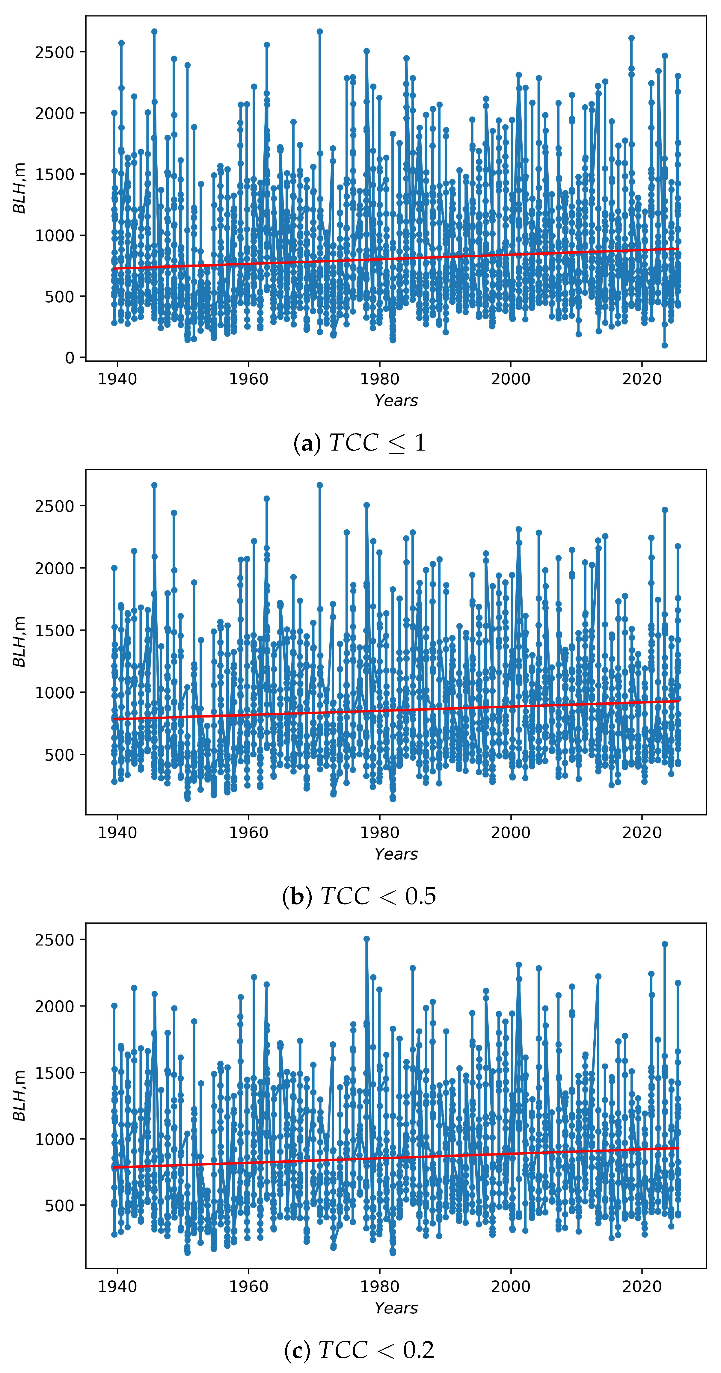
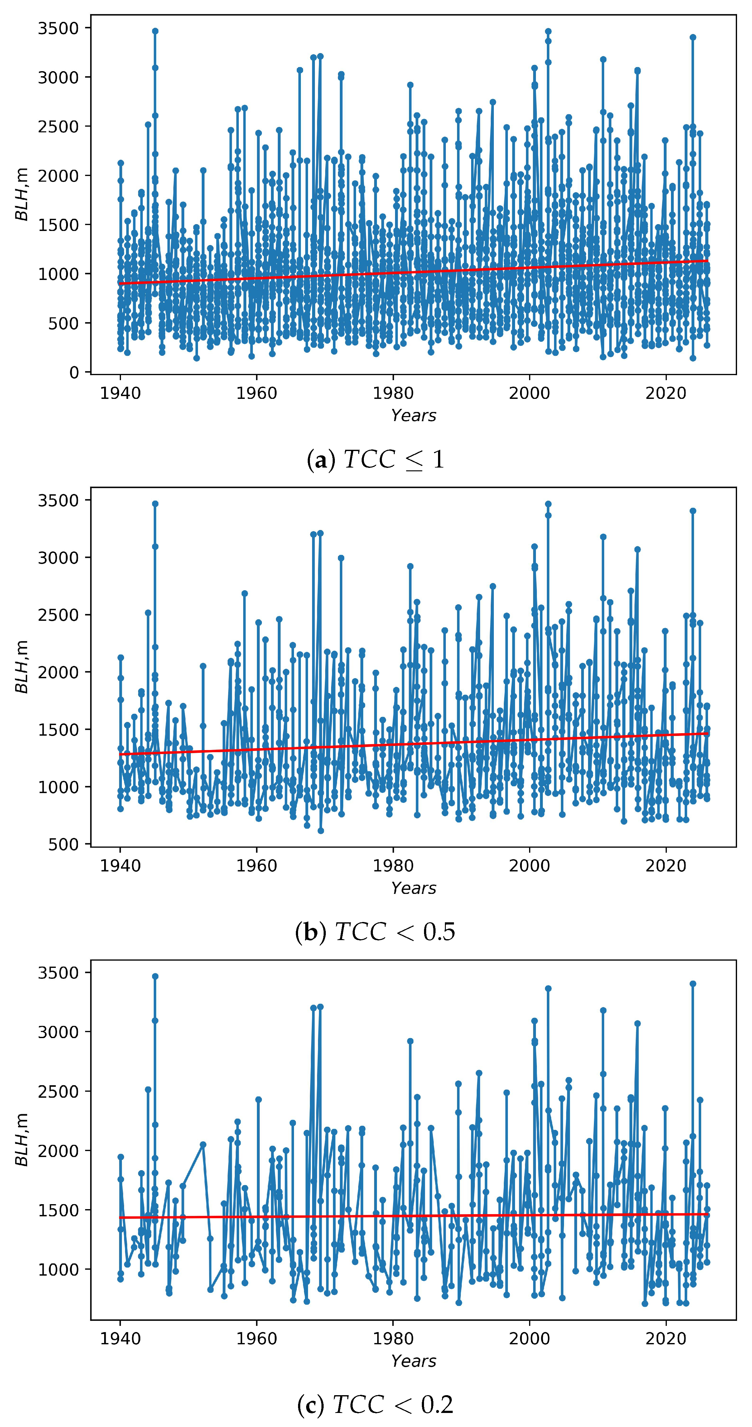
Values of BLH were determined from the ERA-5 reanalysis using hourly values. Figure 8 and Figure 9 show the variations of BLH for different cloud conditions in January and July, respectively, over the period from 1940 to 2025. The trends in changes in BLH, as well as significance indicators (p-value and t-statistic), were estimated. It should be noted that a p-value less than 0.05 or a t-statistic greater than 2 suggests significance and the reliability of the results obtained.
In July (for TCC 1 ), the ERA-5 data show a positive trend in BLH, a B L H = 27 m per decade, standard error is 3.8 m per decade, t = 7.03, p > | t | = 0.0. For TCC < 0.5, coefficient a B L H = 21 m per decade, standard error is 6.6 m per decade, t = 3.19, p > | t | = 0.001. For TCC < 0.2, coefficient a B L H = 3.3 m per decade, standard error is 9.6 m per decade, t = 0.34, p > | t | = 0.73. Thus, these significance indicators show that the trends can be considered representative of cloudy conditions. For clear sky (TCC < 0.2), the trend is not reliable and BLH values have practically no tendency to increase.
In January, a B L H =19 m per decade for TCC 1 , standard error is 3.3 m per decade, t = 5.70, p > | t | = 0.0. For TCC < 0.5, coefficient a B L H = 17 m per decade, standard error is 3.9 m per decade, t = 4.42, p > | t | = 0.0. For TCC < 0.2 coefficient a B L H = 16.9 m per decade, standard error is 4.0 m per decade, t = 4.2, p > | t | = 0.0. Despite the smaller amplitudes of changes (compared with July), these trends are also representative. A comparison of the values of BLH by month shows that the height has a greater tendency to increase in the summer period. This increase is mainly due to changes in cloud cover and, apparently, the water vapor content of the atmosphere.

3.3. Long-Period Changes in Day-Time TCC at HSOS

Cloud cover significantly impacts the possibilities of astronomical observations [30]. It leads to the absorption and scattering of radiation in the optical and infrared spectral ranges, significantly increasing atmospheric opacity in the millimeter and submillimeter ranges. Cloud cover directly determines the available observing time and field of view of astronomical instruments. Low and mid-level clouds are the most critical.
Moreover, the calculated values of r 0 and C n 2 are sensitive to the presence of clouds. On the one hand, air saturated with water vapor is more unstable with respect to the excitation of ascending movements. It should be emphasized that the Fried parameter (at HSOS) tends to increase with decreasing TCC. For example, the median value of the Fried parameter is 3.13 cm for TCC ≤ 0.5 and 4.18 cm for TCC ≤ 0.2.
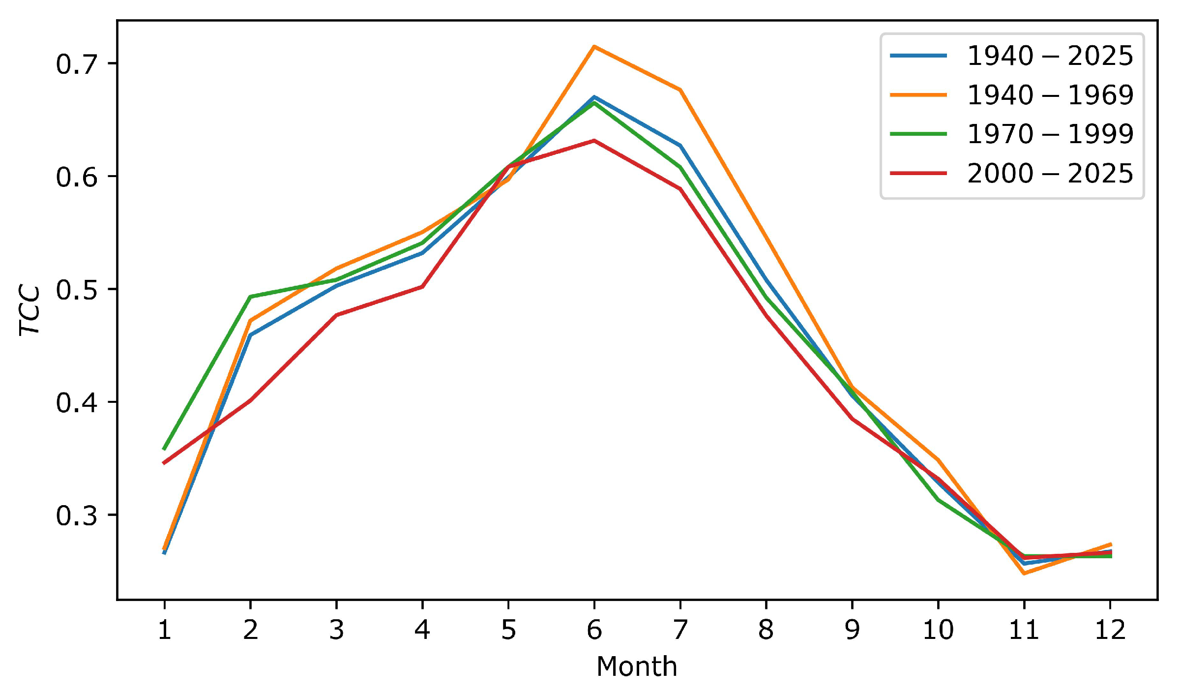
On the other hand, optical distortion measurements based on image scintillation (SCIDAR technology) also contain errors associated with clouds in the upper troposphere. Cloudiness at high levels causes peaks in the scintillation index time series. Seasonal variations in TCC for different time periods are depicted in Figure 10. As can be seen from this figure, the highest pulsations in TCC are observed from January to April as well as in June–July.
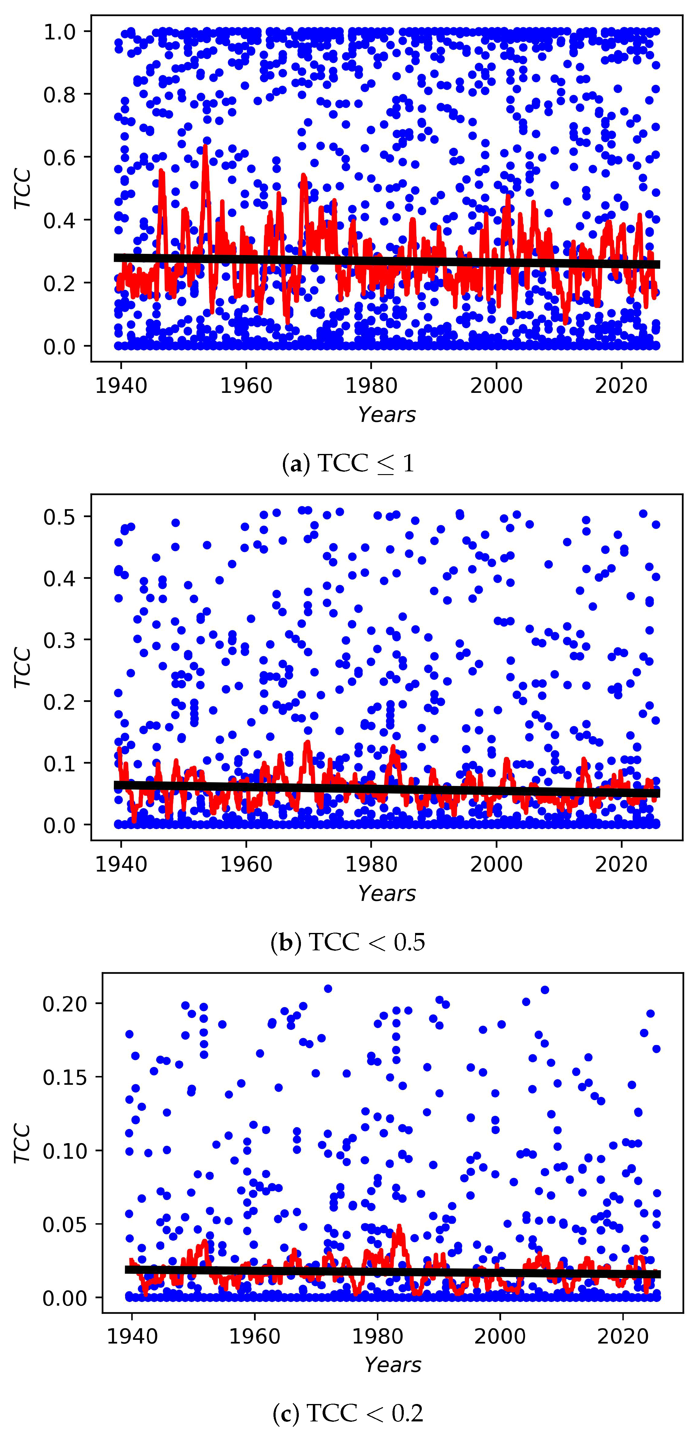
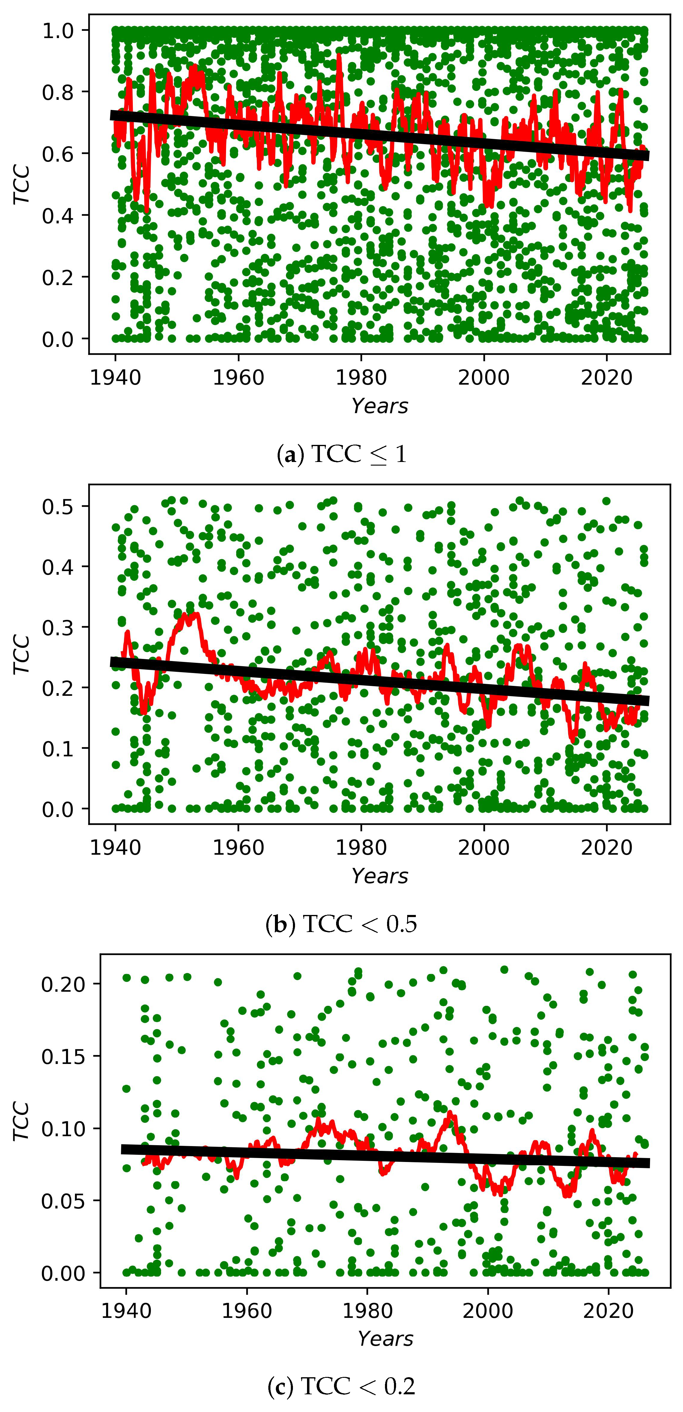
Day-time variations of hourly TCC from ERA-5 from 1940 to 2025 at HSOS in January and July are shown in Figure 11 and Figure 12, respectively. In January, a T C C = −0.002 per decade, t = −0.85, p > | t | = 0.40. For TCC < 0.5, coefficient a T C C = −0.002 per decade, t = −1.46, p > | t | = 0.14. For TCC < 0.2 coefficient a T C C = 0.0 per decade, t = −0.90, p > | t | = 0.37. These estimated changes in total cloudiness for all period are at the error level. In July, an average trend in TCC a T C C = −0.015 per decade, t = −5.50, p > | t | = 0.00. The total decrease in total cloudiness over the past 85 years is about 0.13. For TCC < 0.5, coefficient a T C C = −0.007 per decade, t = −3.64, p > | t | = 0.0. For TCC < 0.2 coefficient a T C C = −0.001 per decade, t = −0.91, p > | t | = 0.36.

4. Discussion

This paper is aimed at studying the atmospheric characteristics relevant for astronomical observations. In particular, characteristic features in the vertical structure of atmospheric optical turbulence above HSOS were revealed. It is shown that over the past 85 years, the intensity of optical turbulence in the atmosphere has changed little. The exception is the lower layer of the atmosphere. The intensity of surface optical turbulence over the period 2000–2025 decreased by ∼20% in January (and by ∼40% in July) compared with the intensity averaged over the period from 1940 to 1969. An increase in turbulence intensity in January at altitudes of 20,000–30,000 m and in July at altitudes of 9000–10,000 m is noteworthy. Apparently, a weak decrease in turbulence in the boundary layer is compensated by its weak increase in the middle-upper troposphere as well as lower stratosphere. As a result, the image quality changes little, on average. It is likely that an increase in turbulence in the upper layers of the Earth’s atmosphere can lead to a decrease in the amount of suspended particles and, as a consequence, a decrease in scattered light.
Characteristic changes in the height of the atmospheric boundary layer, in the layer where intense turbulent fluctuations of the refractive index of air are formed, were estimated. Trends in ERA-5 BLH are positive except in conditions of clear sky.
In TCC, ERA-5 shows negative trends at HSOS. Only the July trend is representative. Its value suggests a decrease in cloud cover of 0.13 over the past 85 years.

5. Conclusions

Profiles of optical turbulence for various time intervals over HSOS were obtained. These vertical profiles were adjusted, taking into account solar observation data at HSOS and the regularities of changes in the parameterization coefficients depending on the integral values of the Fried parameter.
Changes in key astroclimatic characteristics of optical turbulence, atmospheric boundary layer height, and total cloud cover were assessed (for the period from 1940 to 2025). The results indicate a high probability that climate change has already affected atmospheric characteristics over HSOS. It is important to note an interesting effect in long-period changes in the Fried parameter. Comparing two time periods (1940–1969; 2000–2025), it can be concluded that the optical turbulence strength in the lower atmosphere decreased slightly. Despite this decrease, the Fried parameter values for the entire atmosphere changed little. This can be explained by a slight increase in the atmospheric boundary layer height above the station.

Funding

Testing the method for assessing optical turbulence was funded by the RSF grant № 24-72-10043. Measurement data and primary analysis was supported by the Ministry of Science and Higher Education of the Russian Federation.

Institutional Review Board Statement

Not applicable.

Informed Consent Statement

Not applicable.

Data Availability Statement

Data are available upon request.

Acknowledgments

The approaches were previously tested using the Unique Research Facility ”Large Solar Vacuum Telescope” (accessed on 1 November 2025). (http://ckp-rf.ru/usu/200615/).

Conflicts of Interest

The author declares no conflicts of interest.

References

  1. Haslebacher, C.; Demory, M.-E.; Demory, B.-O.; Sarazin, M.; Vidale, P.L. Impact of climate change on site characteristics of eight major astronomical observatories using high-resolution global climate projections until 2050. Astron. Astrophys. 2022, 665, A149. [Google Scholar] [CrossRef]
  2. Cantalloube, F.; Milli, G.; Böhm, C.; Crewell, S.; Navarrete, J.; Rehfeld, K.; Sarazin, M.; Sommani, A. The impact of climate change on astronomical observations. Nat. Astron. 2020, 4, 826–829. [Google Scholar] [CrossRef]
  3. Seidel, J.V.; Otarola, A.; Theron, V. On the Impact of ENSO Cycles and Climate Change on Telescope Sites in Northern Chile. Atmosphere 2023, 14, 1511. [Google Scholar] [CrossRef]
  4. Tillayev, Y.; Azimov, A.; Ehgamberdiev, S.; Ilyasov, S. Astronomical Seeing and Meteorological Parameters at Maidanak Observatory. Atmosphere 2023, 14, 199. [Google Scholar] [CrossRef]
  5. Bolbasova, L.A.; Kopylov, E.A.; Mironov, A.P.; Kokhirova, G.I.; Zhukov, A.O. Variations in the Astroclimate of High-Altitude Observatories of Tajikistan. Astron. Rep. 2025, 69, 999–1008. [Google Scholar] [CrossRef]
  6. Panchuk, V.E.; Afanas’ev, V.L. Astroclimate of Northern Caucasus-myths and reality. Astrophys. Bull. 2011, 66, 233–254. [Google Scholar] [CrossRef]
  7. Zhao, Y.; He, F.; Li, R.; Yang, F.; Deng, L. Variability in Meteorological Parameters at the Lenghu Site on the Tibetan Plateau. Atmosphere 2025, 16, 1210. [Google Scholar] [CrossRef]
  8. Coulman, C.E. Fundamental and applied aspects of astronomical “seeing”. Annu. Rev. Astron. Astrophys. 1985, 23, 19–57. [Google Scholar] [CrossRef]
  9. Fried, D.L. Optical Resolution Through a Randomly Inhomogeneous Medium for Very Long and Very Short Exposures. J. Opt. Soc. Am. 1966, 56, 1372–1379. [Google Scholar] [CrossRef]
  10. Qing, C.; Wu, X.; Li, X.; Luo, T.; Su, C.; Zhu, W. Mesoscale optical turbulence simulations above Tibetan Plateau: First attempt. Opt. Express 2020, 28, 4571–4586. [Google Scholar] [CrossRef]
  11. Bi, C.; Qing, C.; Qian, X.; Luo, T.; Zhu, W.; Weng, N. Investigation of the Global Spatio-Temporal Characteristics of Astronomical Seeing. Remote Sens. 2023, 15, 2225. [Google Scholar] [CrossRef]
  12. Shikhovtsev, A.Y.; Kovadlo, P.G.; Kiselev, A.V.; Eselevich, M.V.; Lukin, V.P. Application of Neural Networks to Estimation and Prediction of Seeing at the Large Solar Telescope Site. Publ. Astron. Soc. Pac. 2023, 135, 014503. [Google Scholar] [CrossRef]
  13. Li, Y.; Zhang, X.; Li, L.; Shi, L.; Huang, Y.; Fu, S. Multistep ahead atmospheric optical turbulence forecasting for free-space optical communication using empirical mode decomposition and LSTM-based sequence-to-sequence learning. Front. Phys. 2023, 11, 11. [Google Scholar] [CrossRef]
  14. Wang, Y.; Basu, S. Using an artificial neural network approach to estimate surface-layer optical turbulence at Mauna Loa. Opt. Let. 2016, 41, 2334–2337. [Google Scholar] [CrossRef]
  15. Jellen, C.; Oakley, M.; Nelson, C.; Burkhardt, J.; Brownell, C. Machine-learning informed macro-meteorological models for the near-maritime environment. Appl. Opt. 2021, 60, 2938–2951. [Google Scholar] [CrossRef]
  16. Shikhovtsev, M.Y.; Obolkin, V.A.; Khodzher, T.V.; Molozhnikova, Y.V. Variability of the Ground Concentration of Particulate Matter PM1PM10 in the Air Basin of the Southern Baikal Region. Atmos. Ocean. Optics. 2023, 36, 655–662. [Google Scholar] [CrossRef]
  17. Kovadlo, P.; Shikhovtsev, A.; Lukin, V.; Kochugova, E. Solar activity variations inducing effects of light scattering and refraction in the Earth’s atmosphere. J. Atmos. Terr. Phys. 2018, 179, 468–471. [Google Scholar] [CrossRef]
  18. Hersbach, H.; Bell, B.; Berrisford, P.; Hirahara, S.; Horányi, A.; Muñoz-Sabater, J.; Nicolas, J.; Peubey, C.; Radu, R.; Schepers, D.; et al. The ERA5 global reanalysis. Q. J. R. Meteorol. Soc. 2020, 146, 1999–2049. [Google Scholar] [CrossRef]
  19. Hu, X.; Yang, S.; Song, T.; Bao, X.; Sun, W.; Deng, Y.; Liu, Y.; Zhao, M. Estimation of Day-Time Seeing Changes at Huairou Solar Observing Station Based on Neural Networks from 1989 to 2010. Universe 2025, 11, 169. [Google Scholar] [CrossRef]
  20. Cuadros, E.T.; Almeida, A.P.; Carlesso, F.; Pareja-Quispe, D.; Guarnieri, F.L.; Lago, A.D.; Gargaglioni, S.R.; Vieira, L.E.A. Assessment of Daytime Sky Quality and Atmospheric Refractive Index ( C n 2 ) Analysis at Pico dos Dias Observatory. Astrophys. J. Suppl. Ser. 2025, 281, 24. [Google Scholar] [CrossRef]
  21. Bi, C.C.; Qing, C.; Qian, X.; Zhu, W.; Luo, T.; Li, X.; Cui, S.; Weng, N. Astroclimatic parameters characterization at lenghu site with ERA5 products. Monthly Notices of the Royal Astronomical Society 2024, 527, 4616–4631. [Google Scholar] [CrossRef]
  22. Liu, Y.; Luo, T.; Yang, K.; Zhang, H.; Zhu, L.; Shao, S.; Cui, S.; Li, X.; Weng, N. Estimation of Atmospheric Boundary Layer Turbulence Parameters over the South China Sea Based on Multi-Source Data. Remote Sens. 2025, 17, 1929. [Google Scholar] [CrossRef]
  23. Dewan, E.M.; Good, R.E.; Beland, R.; Brown, J. A Model for C n 2 (Optical Turbulence) Profiles Using Radiosonde Data; Phillips Laboratory, Directorate of Geophysics, Air Force Materiel Command, Hanscom AFB: Bedford, MA, USA, 1993; Volume 50. [Google Scholar]
  24. Kim, S.-H.; Ueyama, R.; Atlas, R.; Dean-Day, J.; Bui, P.; Smith, J.B.; Podglajen, A.; Homeyer, C.R. Atmospheric Turbulence in the Upper Troposphere and Lower Stratosphere From Airborne Observations During the DCOTSS Field Campaign. JGR Atmos. 2025, 130, e2025JD044556. [Google Scholar] [CrossRef]
  25. Shikhovtsev, A.Y. Reference optical turbulence characteristics at the Large Solar Vacuum Telescope site. Publ. Astron. Soc. Jpn. 2024, 76, 538–549. [Google Scholar] [CrossRef]
  26. Joo, J.Y.; Lee, J.W.; Kim, S.H.; Lee, J.H.; Jung, D.H.; Kim, Y.S.; Park, S.Y.; Butterley, T. One-year Turbulence Profiling Campaign at Geochang Observatory Using a SLODAR. Curr. Opt. Photonics 2025, 9, 468–476. [Google Scholar] [CrossRef]
  27. Quatresooz, F.; Oestges, C. C n 2 Modeling for Free-Space Optical Communications: A Review. IEEE Access 2025, 13, 21279–21305. [Google Scholar] [CrossRef]
  28. Shikhovtsev, A.Y.; Potanin, S.A.; Kopylov, E.A.; Qian, X.; Bolbasova, L.A.; Panchuk, A.V.; Kovadlo, P.G. Simulating Vertical Profiles of Optical Turbulence at the Special Astrophysical Observatory Site. Atmosphere 2024, 15, 1346. [Google Scholar] [CrossRef]
  29. Medeiros, J.D.; Williams, P.D. Future Trends in Upper-Atmospheric Shear Instability from Climate Change. J. Atmos. Sci. 2025, 82, 2375–2392. [Google Scholar] [CrossRef]
  30. Qian, X.; Yao, Y.; Wang, H.; Yin, J.; Yalin, L. C n 2 Statistics of cloud cover above the Ali Observatory, Tibet. Mon. Not. R. Astron. Soc. 2024, 529, 1195–1204. [Google Scholar] [CrossRef]
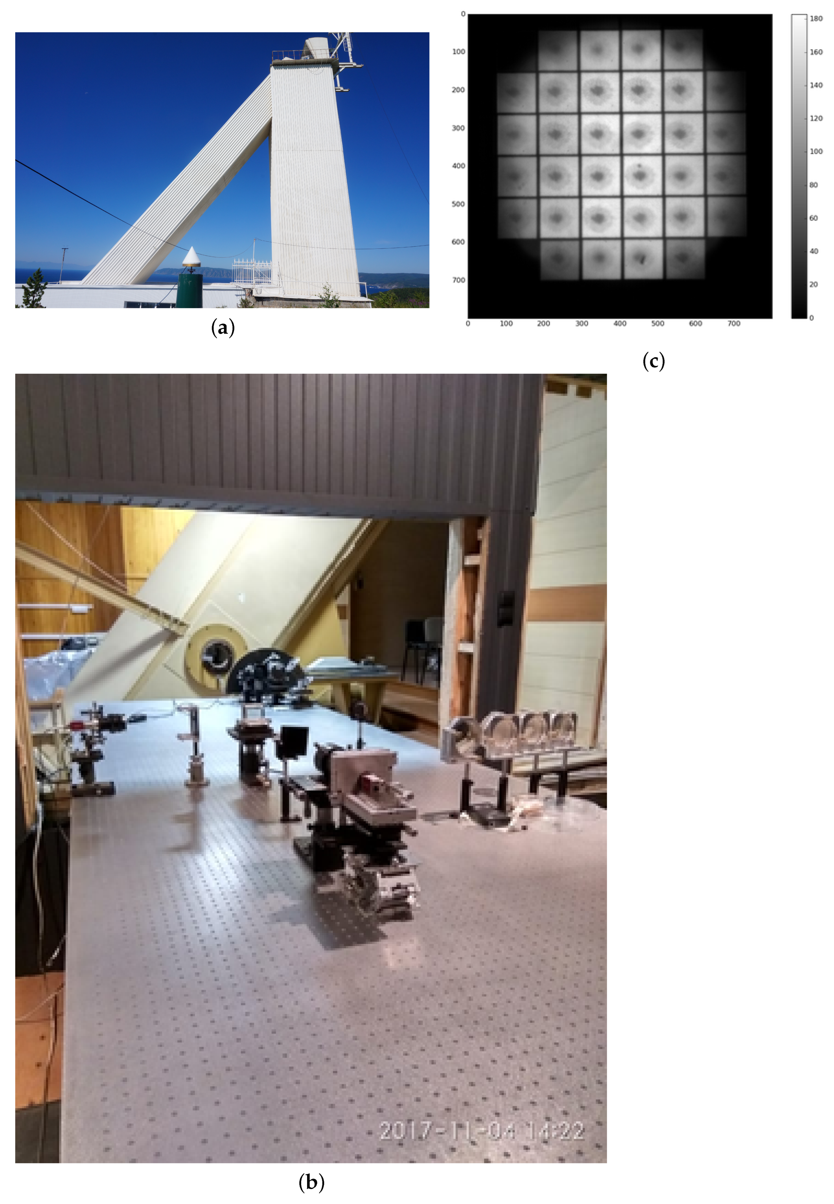
Figure 1. (a) Large Solar Vacuum Telescope; (b) adaptive optics; (c) sunspot Hartmannogram in the second focal plane of LSVT
Universe 12 00011 g001
Figure 2. Comparison of simulated optical turbulence profiles at the Huairou Solar Observing Station. Days with TCC > 0.5 were excluded. The color shading corresponds to the interval between the first and third quartiles.
Universe 12 00011 g002aUniverse 12 00011 g002b
Figure 3. Simulated day-time vertical profiles of optical turbulence strength C n 2 at the Huairou Solar Observing Station in July and January. The color shading corresponds to the interval between the first and third quartiles.
Universe 12 00011 g003
Figure 4. Day-time vertical distributions of F d at the Huairou Solar Observing Station at January and July.
Universe 12 00011 g004
Figure 5. Daytime variations of the meridional gradient of air temperature at a height of 2 m at the HSOS (from January to December). Red line corresponds to smoothed data. Black line indicates the linear regression.
Universe 12 00011 g005
Figure 6. Daytime variations of the zonal gradient of air temperature at a height of 2 m at the HSOS (from January to December). Red line corresponds to smoothed data. Black line indicates the linear regression.
Universe 12 00011 g006
Figure 7. Values of N 2 averaged within atmospheric layer 100–250 hPa at HSOS. Black lines correspond to the linear regression. Yellow and green lines are smoothed pulsations of N 2 for January and July, respectively.
Universe 12 00011 g007
Figure 8. Day-time variations in BLH in January, HSOS. Red lines indicate the linear regression.
Universe 12 00011 g008
Figure 9. Day-time variations in BLH in July, HSOS. Red lines indicate the linear regression.
Universe 12 00011 g009
Figure 10. Seasonal variations in TCC for different time periods.
Universe 12 00011 g010
Figure 11. Day-time variations in TCC from ERA-5 at HSOS (1940–2025, January). The hourly values of TCC have been fitted with linear regression models (shown by black lines). Red lines correspond to smoothed data.
Universe 12 00011 g011
Figure 12. Same as Figure 11 but for July.
Universe 12 00011 g012
Table 1. Parameters of LSVT and optical setup.
ParameterValue
Total aperture diameter760 mm
Entrance aperture size600 mm
Telescope focal length40 m
Light wavelength535 nm
Number of subapertures6 × 6, 8 × 8, 10 × 10
Equivalent size of subaperture100 mm, 75 mm, 60 mm
Angular pixel size0.3″/pix
Frame frequency80–300 Hz
Typical exposure30 ms
Table 2. Parameterization coefficients for different values of the Fried parameter r 0 ( λ = 500 nm).
r 0 , cm A L B dV , s
≤41.98.0
>4 ≤ 61.805.40
>6 ≤ 101.8020.0
>101.6442.0
Table 3. Median values of the Fried parameter r 0 at the LSVT site.
Month123456789101112
Value, cm3.03.34.36.06.26.76.76.65.43.83.33.9
Table 4. Day-time statistics of the Fried parameter (January) from simulation, TCC ≤ 0.5.
Median Value of r 0 Q 1 Q 3
cmcmcm
Period 1989–2010
2.505.131.84
Period 1940–1969
2.485.211.90
Period 1970–1999
2.495.331.75
Period 2000–2025
2.785.401.80
Table 5. Day-time statistics from simulation of the Fried parameter (July) from simulation, TCC ≤ 0.5.
Median Value of r 0 Q 1 Q 3
cmcmcm
Period 1989–2010
2.395.591.85
Period 1940–1969
2.425.401.89
Period 1970–1999
2.505.461.97
Period 2000–2025
3.135.622.10
Disclaimer/Publisher’s Note: The statements, opinions and data contained in all publications are solely those of the individual author(s) and contributor(s) and not of MDPI and/or the editor(s). MDPI and/or the editor(s) disclaim responsibility for any injury to people or property resulting from any ideas, methods, instructions or products referred to in the content.