Gravitational Wave Detection with Angular Deviation of Electromagnetic Waves

Abstract

In this note, we discuss interesting aspects of the interaction of electromagnetic waves (EMW) with gravitational waves (GWs) and how we can use them for GW detection. We show that there is (i) a deviation from the original path of the EMW, as measured by an angle of the scattered EMW, as well as (ii) a change in frequency. We show that the angular deviation is dependent on the frequency of the initial EMW and GW and suggest the use of MASERS/RASERS instead of LASERS for GW detection. We also briefly examine the influence of the Earth’s rotation and revolution, which can be sources of noise in the measurement of the angular deviation of EMW.

1. Introduction

Gravitational waves have opened a new window into understanding the universe and its dynamics [1]. These waves (GWs) interact less than electromagnetic waves (EMWs) and are expected to carry more information from distant events. To date, more than 200 GW events have been detected in the most recent run of LIGO, and the amount of data is unprecedented [1]. New detectors are being planned, including the space-based satellite LISA [2], and it is expected that further refinement of detection methods will allow for new observations. The Einstein Telescope, a third-generation GW detector in Europe, is expected to detect higher-frequency GWs [3]. There are still searches for the primordial GW from the early universe, which have yet to be found [4]. The current detectors observe only one polarization and require greater accuracy as well as sensitivity to a broader range of GW frequencies. The search for higher-frequency stochastic background GWs is also ongoing [5,6]. An interesting discussion on high-frequency GWs can be found in [7]. In this scenario, we investigated interactions of GWs with various matter fields with the hope of increasing the number of methods of GW detection. In [8,9,10,11], we studied the interaction of GWs with scalars, fermions, electromagnetic waves, quarks, and gluons. In the process, we discovered interesting behavior of quark–gluon plasma and the fact that GWs induce quark flavor transitions [11]. In [12], we showed that a static charged particle in the presence of a GW shows a magnetic field, which can be detected by sensitive instruments like SQUIDs or superconducting quantum interference devices [13]. Our calculations are classical and predict new results that are observable. One could, of course, take the matter fields as quantum and keep the GWs classical, but that would be at higher energy scales than what we are studying in this paper. In this paper, we focus on the interaction of the EMW with GWs and find EMW perturbations by solving Maxwell’s equations. Here, the EMWs are plane waves, and their propagation is studied using Maxwell’s equations. The results are important for multi-messenger astronomy, Early Universe Cosmology, and the detection of GWs on Earth. For a recent discussion on EMW, GWs, and multi-messenger astronomy, see [14]. Our results differ from those of previous studies, such as those used in interferometry [15], as we use Maxwell’s equations in a GW background instead of using geometric optics or light propagation in a GW background. There are similar calculations of Maxwell’s equations for EMW and GW interaction and the change in EMW polarization. These have been studied, as shown by Gertsenshtein, as gravitomagnetic transitions [16], and though these effects are similar to our calculations, there are differences in the initial condition assumptions and the specific quantities we study. For a recent study on polarization effects on EMW and their detection, see [17]. Another recent study also used Maxwell’s equations but finds a phenomenon known as quadrirefringence [18]. In [8], we showed that the EMW acquires a small perturbation in the presence of a GW, and we found an exact formula for this. We examine here in further detail the analytical results obtained in [8] for EMW interacting with GWs using realistic values and tried to understand their observational significance. The ‘perturbed’ EMW shows (i) a clear deviation from the original direction and (ii) a change in the frequency of the EMW. The results are different from [17,18] due to the boundary conditions assumed. It is assumed that the GW emitted in the past, modeled by a plane wave, arrives on Earth at t = 0, interacts with an EMW, and generates a perturbation. Thus, at $t=0$, the perturbation is zero, and once it starts, it propagates. Our aim in this paper is to examine the angular deviation and the frequency change, and whether they can be used in GW detection. We do not discuss the implementation of the results in an instrumental setup, such as in an interferometer; however, we suggest novel ways in which the perturbation can be detected by other methods. In particular, we observed that when the GW frequency exceeds the EMW frequency, the perturbation is at right angles to the initial direction. This is a stark effect given the weak GW amplitude, and we discuss the implications of this in designing new methods of GW detection.

The results we present show that the perturbations are frequency-dependent, and the angular deviation of the perturbed EMW from the initial direction is a function of the relative ratio of the initial frequencies of GWs and EMW. It is also noted that for measurable deviations, the frequency of the EMW has to be lower than the frequency of the LASERs used in LIGO. We hope that our results can be verified in a future experiment using MASER (Microwave Amplification by Stimulated Emission of Radiation) [19] or RASER (Radiowave Amplification by Stimulated Emission of Radiation) [20], which have lower frequencies than LASERs. These suggestions are very new, and we hope that when stable MASERs and RASERs are built, future GWs can be detected using these instead of LASERs.

In Section 2, we discuss the physics of the LIGO experiment and how the results of [8] are commensurate with the LIGO observations. We then explore the exact formula of [8] for the EMW perturbation to predict the angular deviation of the EMW perturbation due to the GW in Section 3. We show that our results can be detected in more sensitive instruments, including nano-sensors such as SQUIDs. We also discuss the effect of Earth’s rotation on the measurements of the angular deviation in Section 4. The geodynamic effect identifies one noise effect that the measurements of the angular deviation of the EMW can have. They have not been discussed before for their effect on LASER polarization in GW interferometers. We then conduct a spectral analysis of the EMW perturbation to identify the frequencies. Finally, Section 6 is the conclusion section.

2. Interaction of Gravitational Waves with Electromagnetic Waves

GWs expand and contract space as well as light waves, which causes a redshift or blueshift in light. This change in frequency is, however, not measured in LIGO, nor is any angular deviation of the laser from its initial direction. What is mainly studied instead is the interference due to the change in the arm length of the interferometers, as the metric of space-time fluctuates due to the GW. In the following discussion, we try to show the effect that is measured in LIGO, as this places our calculation in context.

Why Do We Observe Only the Change in Path Length in LIGO?

In a LASER interferometer, there are two arms at right angles. Light travels along the two arms and is reflected by mirrors back to the initial location. When the light waves recombine, if the two perpendicular arms are the same length (i.e., length of x-arm $L_x=L_y=L$, length of y-arm), then the waves will be in phase. If one arm is a different length than the other due to GW interaction (i.e., $L_x\ne L_y$), then there is a phase shift between the two waves, and when they superpose, an interference pattern is generated. In the following, we report on how the phase difference is calculated for detection in LIGO experiments. We take the metric of space-time with a GW to be:

$$d{s}^2=-d{t}^2+\left(1+h_{+}(t,z)\right)d{x}^2+\left(1-h_{+}(t,z)\right)d{y}^2+d{z}^2,$$

(1)

where we have one polarization of the ‘linearized perturbation’ propagating as $h_{+}=A_{+}\cos \left({\omega }_g(t-z)\right)$ in the z-direction with frequency ${\omega }_g$ and amplitude $A_{+}$. In the metric for the GW we discuss in this paper, $h_{\times }$ polarization is absent. The details of the GW solution of Einstein’s equation can be found in reviews [21]. To estimate the phase difference for the x-arm at time $t_0$, in the z = 0 plane, we calculate the length using the above metric (1) [22]:

$$\int ds=\int {[1+A_{+}\cos \left({\omega }_g{t}_0\right)]}^{1/2}dx\to L_x\approx [1+{\displaystyle \frac{A_{+}}{2}}\cos \left({\omega }_g{t}_0\right)]L.$$

(2)

In the last line, we kept terms up to linear order in $A_{+}$. Performing the same process, we find that the y-length is:

$$L_y=[1-{\displaystyle \frac{A_{+}}{2}}\cos \left({\omega }_g{t}_0\right)]L.$$

(3)

The round-trip time for each light wave is simply the arm length multiplied by ${\displaystyle \frac{2}{c}}$. The phase difference for an EMW of frequency ${\omega }_e$ is:

$$\Delta \varphi ={\omega }_e\Delta t\approx \Delta \varphi ={\displaystyle \frac{2L{A}_{+}}{c}}{\omega }_e\cos \left({\omega }_g{t}_0\right).$$

(4)

Next, we calculate the change in wavelength [22].

$${\displaystyle \frac{\Delta \lambda }{\lambda }}={\displaystyle \frac{d}{dt}}[L+{\displaystyle \frac{L{A}_{+}}{2}}\cos \left({\omega }_g{t}_0\right)]{\displaystyle \frac{2L}{c}}{\displaystyle \frac{1}{L}}\approx {\displaystyle \frac{\Delta \lambda }{\lambda }}=-{\displaystyle \frac{L{A}_{+}}{c}}{\omega }_g\sin \left({\omega }_g{t}_0\right).$$

(5)

Similarly, the change in wavelength for the y-arm is $\frac{\Delta \lambda }{\lambda }={\displaystyle \frac{L{A}_{+}}{c}}{\omega }_g\sin \left({\omega }_g{t}_0\right)$.

Hence, we can see that the phase shift depends on the frequency of the light, whereas the change in wavelength depends on the frequency of the GW. The frequency of the GW is approximately 1000 rad/sec, and the frequency of the light is roughly ${10}^{15}$ rad/sec, as is typical in the LIGO interferometer [15]. Thus, ${\omega }_e>>{\omega }_g$, and hence, the phase shift is a much larger physical effect. If we wish to measure the change in wavelength, then one way is to make the frequency of light and the frequency of the GW similar, that is, to perform the measurement using radio waves. We expect the instruments to improve and eventually provide coherent waves of microwave and radio waves (MASERs and RASERs). MASERs that operate at 9.2 GHz and RASERs that operate at 600 M Hz exist, but once there is a collimated beam of these, we should be able to detect the redshift or change in the wavelength of the EMW in LIGO detectors using interference mechanisms. In the next section, we discuss an interesting effect observed in [8,9], where Maxwell’s equations were solved to obtain exact results.

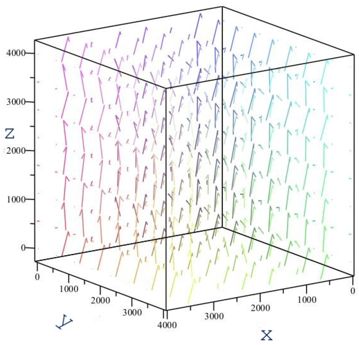
3. Angle Perturbations

In this section, we analyze the ‘change in angle’ perturbation effect of the EMW caused by GWs and produce plots of the angular deviation ($\arctan (T_{0z}/T_{0x})$) (AD) using data for GW170814 for the results of [8]. The advantage of this calculation is that the perturbation of the EMW due to the passing of a GW is calculated using linearized Maxwell’s equations and Green’s function. The gauge potential fields are solved explicitly with appropriate boundary conditions, and the electric and magnetic fields are obtained from the calculations. The Poynting vector obtained in [8] has information on the direction of propagation of the perturbation. The change in angle or deviation of the Poynting vector from the original direction is obtained and plotted as a function of the frequencies of the waves. The initial magnetic field is taken as $\overrightarrow{B}=B_{0y}\cos \left({\omega }_e(x-t)\right)\widehat{y}$ for an EMW propagating in the x-direction with amplitude $B_{0y}$.

In the presence of a GW, the background metric of the EMW changes to that given in Equation (1). Maxwell’s equations are written in this background, and as shown in [8], keeping terms linear in $A_{+}$ and using Lorenz gauge, one obtains (c = 1, $\square =-{\mathsf{\partial }}_t^2+{\mathsf{\partial }}_z^2$):

$$\begin{array}{ccc}\hfill \square {\tilde{A}}_x& =& -A_{+}{B}_{0y}{\omega }_g\sin ({\omega }_{g}z-{\omega }_{g}t)\cos ({\omega }_{e}x-{\omega }_{e}t),\hfill \end{array}$$

(6)

$$\begin{array}{ccc}\hfill \square {\tilde{A}}_z& =& A_{+}{\omega }_e\sin ({\omega }_{e}x-{\omega }_{e}t)\cos ({\omega }_{g}z-{\omega }_{g}t).\hfill \end{array}$$

(7)

where we have assumed that the gauge vector is of the form

$$A_{\mu }=A_{\mu }^0+{\tilde{A}}_{\mu }.$$

(8)

$A_{\mu }^0$ is taken to represent an EMW plane wave in the x-direction. It is given in terms of a nonzero magnetic field amplitude $B_{0y}$.

$$A_z^0=-{\displaystyle \frac{1}{{\omega }_e}}{B}_{0y}\sin ({\omega }_{e}x-{\omega }_{e}t).$$

(9)

As can be seen, only two components of the perturbation field ${\tilde{A}}_{\mu }$ are generated by the GW. The other components are unaffected. The solution to the above with the boundary condition ${\tilde{A}}_{\mu }(t=0)=0$ is found in [8]. They are explicitly:

$$\begin{array}{ccc}\hfill {\tilde{A}}_x& =& {\displaystyle \frac{B_{0y}{A}_{+}}{4{\omega }_e\sqrt{{\omega }_g^2+{\omega }_e^2}}}\left[({\omega }_e+{\omega }_g)\cos ({\omega }_{e}x+{\omega }_{g}z)\sin \left(t\sqrt{{\omega }_e^2+{\omega }_g^2}\right)\right.\hfill \\ & & -\sqrt{{\omega }_g^2+{\omega }_e^2}\sin ({\omega }_{e}x+{\omega }_{g}z)\cos \left(t\sqrt{{\omega }_g^2+{\omega }_e^2}\right)\hfill \\ & +& ({\omega }_e-{\omega }_g)\cos ({\omega }_{e}x-{\omega }_{g}z)\sin \left(t\sqrt{{\omega }_e^2+{\omega }_g^2}\right)-\sqrt{{\omega }_g^2+{\omega }_e^2}\sin ({\omega }_{e}x-{\omega }_{g}z)\cos \left(t\sqrt{{\omega }_e^2+{\omega }_g^2}\right)\hfill \\ & +& \left.\sqrt{{\omega }_g^2+{\omega }_e^2}\sin ({\omega }_{e}x+{\omega }_{g}z-t({\omega }_g+{\omega }_e))+\sqrt{{\omega }_g^2+{\omega }_e^2}\sin ({\omega }_{e}x-{\omega }_{g}z+t({\omega }_e-{\omega }_g))\right].\hfill \end{array}$$

(10)

The solution for ${\tilde{A}}_z$ can be obtained by phase shifts of ${\omega }_{e}x\to {\omega }_{e}x+\pi /2$ and ${\omega }_{g}z\to {\omega }_{g}z+\pi /2$ (these account for the difference in RHS) and by changing the prefactor $B_{0y}{A}_{+}/\left(4{\omega }_e\sqrt{{\omega }_e^2+{\omega }_g^2}\right)\to B_{0y}{A}_{+}/\left(4{\omega }_g\sqrt{{\omega }_e^2+{\omega }_g^2}\right)$.

What is interesting is that, apart from the usual perturbation of the original $A_z$, a component perpendicular to this is generated. This is not there in the phase change and redshift calculations of [1,15] discussed in the previous section.

The perturbation electric field ${\tilde{E}}_x$, which is generated from the solution by deriving ${\tilde{A}}_x$ in time, is:

$$\begin{array}{ccc}\hfill {\tilde{E}}_x& =& {\displaystyle \frac{B_{0y}{A}_{+}}{4{\omega }_e}}\left[({\omega }_e+{\omega }_g)\cos ({\omega }_{e}x+{\omega }_{g}z)\cos \left(t\sqrt{{\omega }_e^2+{\omega }_g^2}\right)\right.\hfill \\ & +& \sqrt{{\omega }_g^2+{\omega }_e^2}\left(\sin ({\omega }_{e}x+{\omega }_{g}z)\sin \left(t\sqrt{{\omega }_g^2+{\omega }_e^2}\right)+\sin ({\omega }_{e}x-{\omega }_{g}z)\sin \left(t\sqrt{{\omega }_e^2+{\omega }_g^2}\right)\right)\hfill \\ & +& ({\omega }_e-{\omega }_g)\cos ({\omega }_{e}x-{\omega }_{g}z)\cos \left(t\sqrt{{\omega }_e^2+{\omega }_g^2}\right)-({\omega }_g+{\omega }_e)\cos ({\omega }_{e}x+{\omega }_{g}z-t({\omega }_g+{\omega }_e))\hfill \\ & -& \left.({\omega }_e-{\omega }_g)\cos ({\omega }_{e}x-{\omega }_{g}z-t({\omega }_e-{\omega }_g))\right].\hfill \end{array}$$

(11)

A perturbed magnetic field is not generated by a + polarized GW. This can be verified by calculating the magnetic field using ${\tilde{B}}_i={ϵ}_{ijk}{\mathsf{\partial }}_j{A}_k$. To generate the magnetic field, the GW must have a $h_{\times }$ polarization term. The perturbed magnetic field then can also be similarly obtained due to the GW, as in [8], if the $h_{\times }=A_{\times }\cos ({\omega }_g(t-z)+\delta )$ mode is present ($\delta$ is a phase shift). Without going into the details of the derivation, one finds in [8] that a magnetic field is generated in the z-direction of the form:

$$\begin{array}{ccc}\hfill {\tilde{B}}_z& =& {\displaystyle \frac{B_{0y}{A}_{\times }}{4\sqrt{{\omega }_g^2+{\omega }_e^2}}}\left[-({\omega }_e+{\omega }_g)\sin ({\omega }_{e}x+{\omega }_{g}z+\delta )\sin \left(t\sqrt{{\omega }_e^2+{\omega }_g^2}\right)\right.\hfill \\ & -& \sqrt{{\omega }_g^2+{\omega }_e^2}\cos ({\omega }_{e}x+{\omega }_{g}z+\delta )\cos \left(t\sqrt{{\omega }_g^2+{\omega }_e^2}\right)\hfill \\ & -& ({\omega }_e-{\omega }_g)\sin ({\omega }_{e}x-{\omega }_{g}z+\delta )\sin \left(t\sqrt{{\omega }_e^2+{\omega }_g^2}\right)\hfill \\ & -& \sqrt{{\omega }_g^2+{\omega }_e^2}\cos ({\omega }_{e}x-{\omega }_{g}z+\delta )\cos \left(t\sqrt{{\omega }_e^2+{\omega }_g^2}\right)\hfill \\ & +& \sqrt{{\omega }_e^2+{\omega }_g^2}\cos ({\omega }_{e}x+{\omega }_{g}z+\delta -t({\omega }_g+{\omega }_e))\hfill \\ & +& \left.\sqrt{{\omega }_e^2+{\omega }_g^2}\cos ({\omega }_{e}x-{\omega }_{g}z+\delta -t({\omega }_e-{\omega }_g))\right].\hfill \end{array}$$

(12)

As one can see, the perturbation is proportional to the product of both $B_{0y}$ and $A_{+}$ and/or $A_{\times }$. Furthermore, due to the generation of an electric field in the x-direction, the fields are no longer transverse to the direction of propagation. To find the propagation of the perturbed EMW field, we calculate the Poynting vector components $S_i$ of the perturbation solution as the $T^{0i}$ components of the energy–momentum tensor. Another interesting aspect of the above result is the oscillatory functions in $\sqrt{{\omega }_e^2+{\omega }_g^2}$ in the electric field. These modes were first observed in [9], and these are solutions to the homogeneous Maxwell’s equations. They appear in the complete solution so as to ensure that the perturbations are zero at $t=0$. The modes are therefore used to implement the boundary conditions to Maxwell’s equations in the GW background. They cannot be interpreted as a redshift, as induced by the analysis of the previous section, and therefore, they represent an interesting result. The interferometers can be designed to test for these new frequencies in the scattered LASER beam. If one uses MASERs and RASERs, the new frequencies in the EMW spectrum will be relevant in the interferometric analysis. The EM energy–momentum tensor of the EMW is given by:

$$T^{\mu \nu }=-{\displaystyle \frac{1}{4\pi }}\left(g^{\mu \alpha }{F}_{\alpha \lambda }{F}^{\lambda \nu }-{\displaystyle \frac{1}{4}}{g}^{\mu \nu }{F}_{\alpha \beta }{F}^{\alpha \beta }\right).$$

(13)

where $F_{\mu \nu }$ is the field strength of the gauge field. Setting specific indices, one obtains the components as:

$$\begin{array}{ccc}\hfill T^{01}& =& {\displaystyle \frac{1}{4\pi }}\left((1-h_{+})((1+h_{+})F_{02}{F}_{21}+F_{31}{F}_{03})\right),\hfill \end{array}$$

(14)

$$\begin{array}{ccc}\hfill T^{02}& =& {\displaystyle \frac{1}{4\pi }}\left((1-h_{+})(1+h_{+})F_{12}{F}_{01}+(1+h_{+})F_{32}{F}_{02}\right),\hfill \end{array}$$

(15)

$$\begin{array}{ccc}\hfill T^{03}& =& {\displaystyle \frac{1}{4\pi }}\left((1-h_{+})F_{13}{F}_{01}+(1+h_{+})F_{23}{F}_{02}\right).\hfill \end{array}$$

(16)

At the linearized level, the energy–momentum nonzero components are in the original x-direction and in the z-direction. If we compute them explicitly, then $h_{\times }$ is zero in this calculation:

$$\begin{array}{ccc}\hfill T^{0x}& =& {\displaystyle \frac{1}{4\pi }}[B_{0y}^2{\cos }^2({\omega }_{e}x-{\omega }_{e}t)(1-A_{+}\cos ({\omega }_{g}z-{\omega }_{g}t))\hfill \\ & +& {\displaystyle \frac{B_{0y}^2{A}_{+}\cos ({\omega }_{e}x-{\omega }_{e}t)}{4{\omega }_e{\omega }_g}}\{\left({\displaystyle \frac{{\omega }_g^3-2{\omega }_e^3-{\omega }_e^2{\omega }_g}{\left|\right|\omega \left|\right|}}\right)\sin ({\omega }_{e}x+{\omega }_{g}z)\sin \left(\right|\left|\omega \right|\left|t\right)\hfill \\ & -& \left({\displaystyle \frac{{\omega }_e^2{\omega }_g-2{\omega }_e^3-{\omega }_g^3}{\left|\right|\omega \left|\right|}}\right)\sin ({\omega }_{e}x-{\omega }_{g}z)\sin \left(\right|\left|\omega \right|\left|t\right)\hfill \\ & +& \left({\omega }_g^2-2{\omega }_e^2-{\omega }_g{\omega }_e\right)\cos ({\omega }_{e}x+{\omega }_{g}z)\cos \left(t\right|\left|\omega \right|\left|\right)\hfill \\ & -& \left({\omega }_g^2-2{\omega }_e^2+{\omega }_g{\omega }_e\right)\cos ({\omega }_{e}x-{\omega }_{g}z)\cos \left(t\right|\left|\omega \right|\left|\right)+\left({\omega }_g^2-2{\omega }_e^2+{\omega }_g{\omega }_e\right)\cos ({\omega }_{e}x-{\omega }_{g}z-t\tilde{\omega })\hfill \\ & -& \left({\omega }_g^2-2{\omega }_e^2-{\omega }_e{\omega }_g\right)\cos ({\omega }_{e}x+{\omega }_{z}z-t\overline{\omega })\}],\hfill \end{array}$$

(17)

where we have used the notation $\left|\right|\omega \left|\right|=\sqrt{{\omega }_e^2+{\omega }_g^2}$ and $\overline{\omega }={\omega }_e+{\omega }_g$ and $\tilde{\omega }={\omega }_e-{\omega }_g$. The other nonzero component is:

$$\begin{array}{ccc}\hfill T^{0z}& =& -{\displaystyle \frac{B_{0y}^2{A}_{+}}{16\pi {\omega }_e}}\cos ({\omega }_{e}x-{\omega }_{e}t)[\overline{\omega }\cos ({\omega }_{e}x+{\omega }_{g}z)\cos \left(\right|\left|\omega \right|\left|t\right)+\tilde{\omega }\cos ({\omega }_{e}x-{\omega }_{g}z)\cos \left(\right|\left|\omega \right|\left|t\right)\hfill \\ & +& \left|\right|\omega \left|\right|\left(\sin ({\omega }_{e}x+{\omega }_{g}z)+\sin ({\omega }_{e}x-{\omega }_{g}z)\right)\sin \left(\right|\left|\omega \right|\left|t\right)-\overline{\omega }\cos ({\omega }_{e}x+{\omega }_{g}z-t\overline{\omega })\hfill \\ & -& \tilde{\omega }\cos ({\omega }_{e}x-{\omega }_{g}z-t\tilde{\omega })].\hfill \end{array}$$

As mentioned in the introduction, in this paper, we focus on the nature of the angular deviation (AD) of the perturbation. The angle of perturbation is found using the nonzero components of the energy–momentum tensor and is given by

$$\theta =\arctan \left({\displaystyle \frac{T^{0z}}{T^{0x}}}\right).$$

(18)

Using the values provided by LIGO for GW170814 [23], Figure 1 describes the change in angle during the interaction with LIGO’s LASER and a GW. Figure 2 describes a hypothetical change in angle during the interaction of a GW with the frequency value of the MASER. The magnitude of the angular perturbation is determined by the order of magnitude of the amplitude of the GW. In this case, the peak strain of GW170814 was observed to be $6\times {10}^{-22}$. In both figures, a drastic spiking phenomenon is observed. The feature of dramatic spikes occurs at the limit:

$${\mathrm{Limit}}_{T^{0x}\to 0}\arctan \left({\displaystyle \frac{T^{0z}}{T^{0x}}}\right).$$

(19)

Mathematically, this occurs because $\arctan \left(\frac{1}{x}\right)$ is discontinuous at $x=0$ and because $T^{0x}$ approaches zero at a greater rate than $T^{0z}$.

While the plot for the maser oscillates between positive and negative values, the plot for LIGO is strictly negative. This occurs because over the given timescale, $T^{0z}$ is negative. However, plotting $\theta$ over a timescale of 1 s in Figure 3, we observe that the plots begin to trend into the positive quadrant. As is evident, there are interesting features in the angle the EMW makes with the initial direction as a function of time, and these can be measured in a sensitive detector. The above can also be used to measure the frequency of the perturbed EMW as the angle fluctuates as a function of the frequency.

Figure 4 shows the angular deviation of an EMW with the same order of frequency as the GW in GW170814.

Next, using the equations of the E and B fields interacting with the GW described in [8], we provide the FIELD plots of the Poynting vector due to GW interactions for LIGO’s laser as well as other hypothetical detector frequencies in Figure 5, Figure 6, Figure 7 and Figure 8. The value of $B_{0y}$ was taken to be 1.

The deviation of the Poynting vector is proportional to the frequency ratio of the detector and the GW. We used the data for GW170814, which has a frequency of ∼179 Hz and propagates in the z-direction. At LIGO’s frequency (282T Hz) [23], we can see from Figure 5 that there is no significant deviation in the z-direction. When the Poynting vector is plotted for a hypothetical detector using a MASER with a frequency of ∼9 GHz [19], we begin to see the field deviating, as seen in Figure 6. The amplitudes of the vector field components have been scaled to obtain an emergent graph. Further deviation is observed in Figure 7 when the detector’s frequency has the same order of magnitude as the EM wave (∼300 Hz). When ${\omega }_g>{\omega }_e$, the EM wave becomes perpendicular to the original direction, as shown in Figure 8.

These are instantaneous snapshots of the field. If one takes a time average of the Poynting vector, a net angular deviation is found, as shown in [8].

Evidently, when the EMW and GW have frequencies of the same order, we expect to see tangible effects of AD, and this should be detected. These effects are different than the phase shift currently observed in LIGO.

4. Geodynamic Effects on Angle Measurement

In the previous section, we saw that a perturbed EMW deviates from its original direction due to a GW. In this section, we discuss the effects that Earth’s motion has on the detection of the AD produced by the GW. The magnitude of the AD caused by the GW is proportional to the amplitude of the GW, as shown in Section 3, which was of the order of ${10}^{-19}..{10}^{-22}$ radians in the case of GW170814. Angular changes due to Earth’s motion need to be taken into account when designing an experiment, as the magnitude of the deviation is so small. When considering the geodynamics of the system, there are three factors that have an effect on the system. Earth’s rotation, Earth’s revolution around the sun, and the precession of Earth’s axis are the effects, in order from largest to smallest. In general, various effects of Earth’s geodynamics on GW detection have been analyzed as ‘noise’ in the data, e.g., seismic attenuation [24]; here, we are analyzing the ‘noise’ Earth’s rotation can bring to the GW AD data. There are also detailed studies of Earth’s rotation and GW observations by the Einstein Telescope [25], but here, we are concerned about a very specific effect, namely AD.

Using a simple ratio of angle and period, we can approximate the angular change to the system by each of the effects mentioned above:

$${\theta }_e={\displaystyle \frac{2\pi }{{\tau }_e}}·t_{gw}.$$

(20)

In the equation, ${\theta }_e$ represents the angular change due to the effect, ${\tau }_e$ represents the period of the effect, and $t_{gw}$ is the timescale of the GW. Using this ratio again with respect to GW170814 yields Earth’s rotation (${\theta }_{rot}\approx 1.96\times {10}^{-5}$ rad), Earth’s revolution around the sun (${\theta }_{rev}\approx 5.38\times {10}^{-8}$ rad), and the precession of Earth’s axis (${\theta }_{prec}\approx 2.09\times {10}^{-12}$ rad). This is by no means rigorous and is only being used to demonstrate the magnitudes of each effect relative to the amplitude of the GW, and in experiments, a more precise development of angular change over time due to the geodynamic factors should be carried out. Ignoring the two factors (${\theta }_{rev}$ and ${\theta }_{prec}$) for a moment, we predict that if the detector is designed such that the laser’s propagation is parallel to the axis of Earth’s rotation, then the only factor in the deviation angle is the GW (again, we are ignoring ${\theta }_{rev}$ and ${\theta }_{prec}$ for now). In an inertial reference frame, the AD of the LASER due to the GW will remain unchanged for the duration. However, in the detector’s rotating reference frame, the deviation angle will rotate in accordance with Earth’s revolution. Therefore, to analyze the AD data, the revolution of Earth for the duration of the GW would need to be subtracted to achieve an inertial reference frame. By aligning the LASER’s propagation with the axial tilt, we are negating the largest factor; however, the effects of the rotation around the sun and the precession of Earth’s axis are still non-negligible effects, as they are still orders of magnitude larger than the change in angle due to the GW.

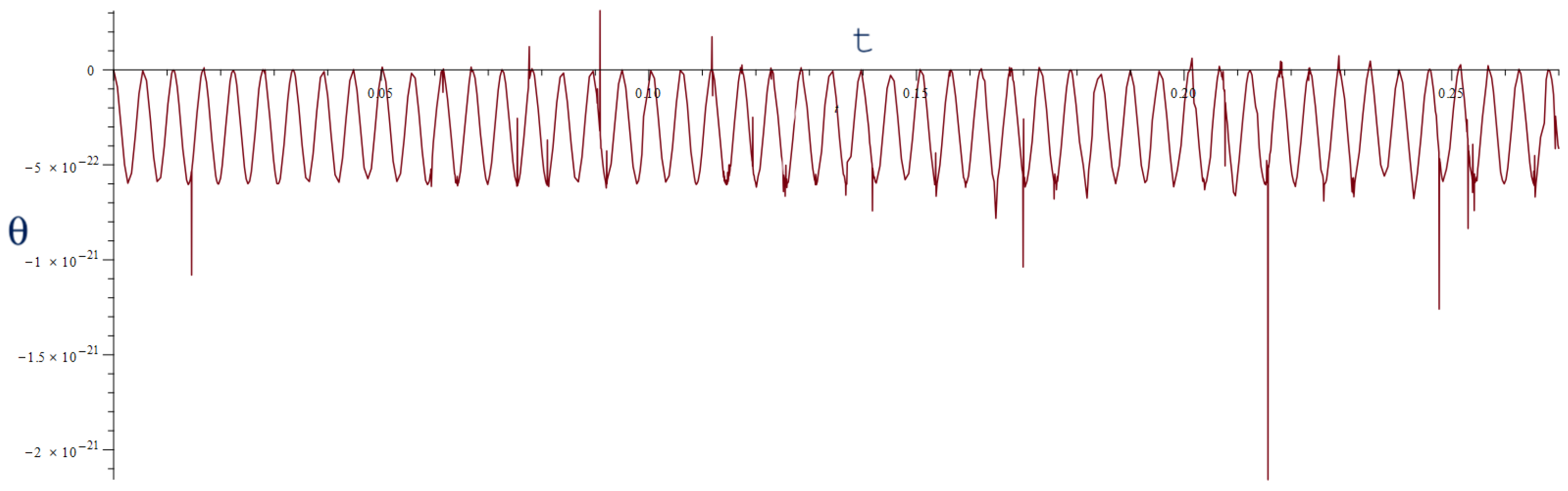
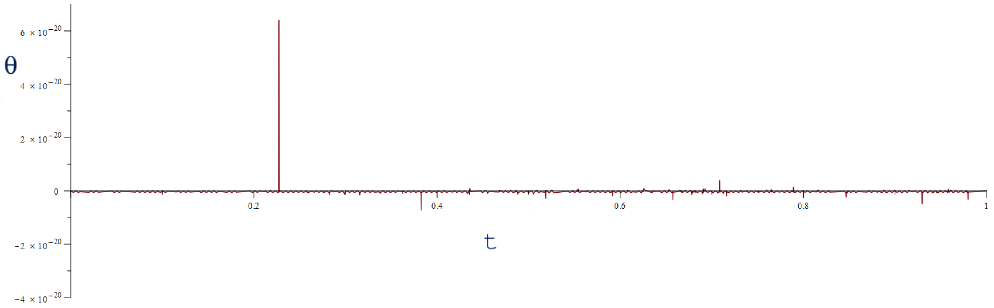
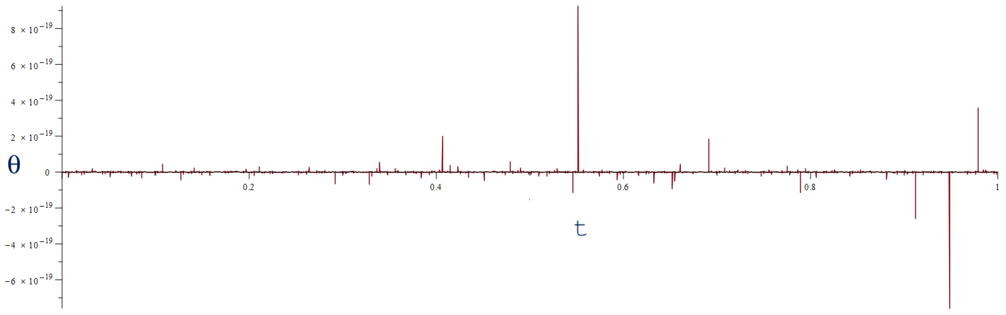
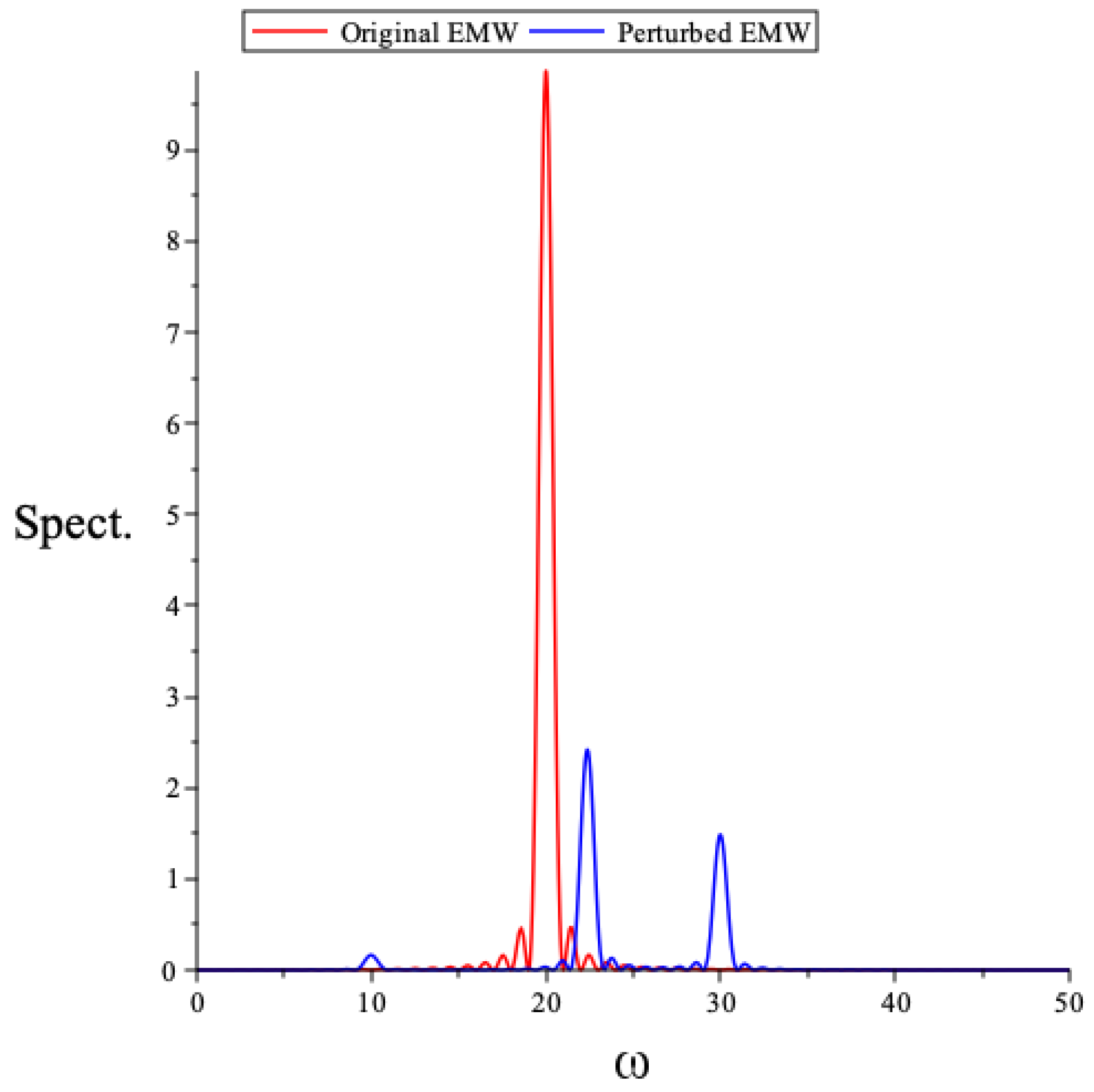
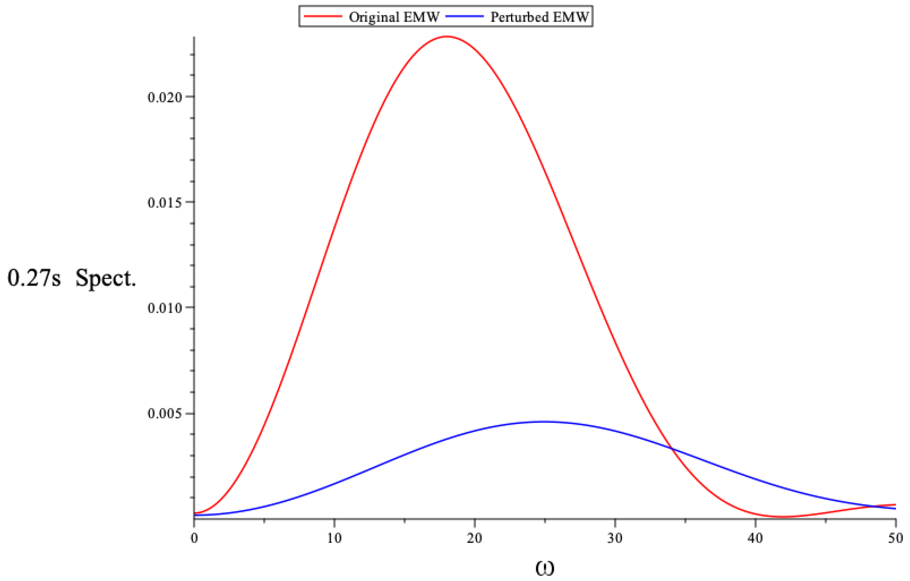
5. Spectral Analysis of the Scattered Beam

In this section, we discuss the spectrum of the perturbations. If we use the electric field generated due to the perturbation, let us say the x-component, then the Fourier analysis can be conducted very easily. The electric field interacts with the electron in the detector, and therefore, the ‘frequency’ of light information is carried by the electric field. If we make a Fourier transform of the perturbation of the electric field, as in Equation (11), we obtain the delta function for the frequencies at $\omega =\pm \sqrt{{\omega }_e^2+{\omega }_g^2},\pm \overline{\omega },\pm \tilde{\omega }$. The coefficients of the delta functions are $E\left(\omega \right)$, which appear in the power spectrum. We thus have the coefficients as:

$$\begin{array}{ccc}\hfill E_x(\pm \sqrt{{\omega }_e^2+{\omega }_g^2})& =& {\displaystyle \frac{B_{0y}{A}_{+}}{8{\omega }_e}}\left[\overline{\omega }\cos ({\omega }_{e}x+{\omega }_{g}z)+\tilde{\omega }\cos ({\omega }_{e}x+{\omega }_{g}z)\right.\hfill \\ & & \left.\mp ı\left|\right|\omega \left|\right|(\sin ({\omega }_{e}x+{\omega }_{g}z)+\sin ({\omega }_{e}x-{\omega }_{g}z))\right],\hfill \end{array}$$

(21)

$$\begin{array}{ccc}\hfill E_x(\pm \overline{\omega })& =& \mp {\displaystyle \frac{B_{0y}{A}_{+}\overline{\omega }}{8{\omega }_e}}𝚤\sin ({\omega }_{e}x+{\omega }_{g}z),\hfill \end{array}$$

(22)

$$\begin{array}{ccc}\hfill E_x(\pm \tilde{\omega })& =& {\displaystyle \frac{B_{0y}{A}_{+}\tilde{\omega }}{8{\omega }_e}}𝚤\sin ({\omega }_{e}x-{\omega }_{g}z).\hfill \end{array}$$

(23)

Graphically, we show the spectral analysis of the perturbed electric field compared to the original signal in Figure 9 and Figure 10. As the frequencies of GW170814 are difficult to implement in a plot, we take ${\omega }_g=10\mathrm{rad}/\mathrm{s},{\omega }_e=20\mathrm{rad}/\mathrm{s}$, and the amplitudes as 1. In a complete cycle of the wave, the perturbed $\tilde{E}$ field frequencies peak at 10 rad/s, $10\sqrt{5}$ rad/s, and 30 rad/s, as shown in Figure 9. When the spectral analysis is for only T = 0.27 s, as that was the duration of the GW signal, we obtain a much broader spectrum, as shown in Figure 10. Unlike the original signal, the frequency dependence of the perturbation is inversely proportional to the ${\omega }_e$, which is also reflected in the plots. However, as the perturbation propagates even after the GW stops after 0.27 s, we expect the full cycle analysis to be relevant for the observations, as shown in Figure 9.

In the spectral analysis of the system, we take the energy of the EM wave and use Parseval’s theorem to write the power in Fourier transform space. However, one has to use the details of GW170814, including the GW frequency (${\omega }_g={10}^3$ rad/s and ${\omega }_e={10}^{15}$ rad/s) and the fact that the GW signal lasts only 0.27 s. What we have succeeded in showing, though, is that, theoretically, the EMW will change from a monochromatic wave to a spectrum under the influence of a GW. The actual effect of this in an interferometer has to be obtained using further calculations, including the beam splitter, which is crucial. We have work in progress in this direction.

6. Conclusions

In this article, we analyzed the effect of a GW on a LASER and a MASER wave and found that the frequencies of the EMW and GWs are important in the results. In particular, the detection of the AD due to the perturbation of the EMW was discussed, which is dependent on the ratio of the frequencies. It was found that the AD is of the order of ${10}^{-21}$ radians for a LASER beam, as expected, and one can detect it in a precision instrument after accounting for Earth’s rotation. We also predict that the use of a lower-frequency EMW source like the MASER/RASER will facilitate the detection of angular deviation, as well as changes in frequency, in a more accurate way. We found that the ratio of frequency can offset the amplitude, and in some regions, the perturbation theory would break down. The plot of the AD thus has to be derived for non-perturbative Einstein–Maxwell’s equations, with the GW as an initial boundary condition for Einstein’s equations. In addition, it is evident from the formula for the perturbed electric field (11) that the power spectrum peaks at three different frequencies: $\tilde{\omega },\overline{\omega },and\left|\right|\omega \left|\right|$. The monochromatic EMW is thus scattered by the GW, and this ‘spectrum’ can be measured. The different frequencies in the spectrometry of the scattered EMW can be detected when ${\omega }_e\approx {\omega }_g$, i.e., the EMW is either a MASER or a RASER for the frequency range of the GW detected in LIGO. We think that the use of polarizers and nano-sensors like SQUIDs to detect changes in the electric and magnetic fields in the scattered light wave will prove useful. These quantum sensors are sensitive to changes in magnetic fields up to an accuracy of $\sim {10}^{-20}$ T. This is precisely the order of the electric and magnetic field perturbations induced by the GW we discussed in this paper. In the future, GWs will be used in new technology and for practical purposes, such as in health, and the devices will be microscopic.

References

1. The LIGO Scientific Collaboration Publications. Available online: https://pnp.ligo.org/ppcomm/Papers.html (accessed on 25 May 2025).
2. The LISA Interferometer. Available online: https://lisa.nasa.gov/ (accessed on 25 May 2025).
3. Abac, A.; Abramo, R.; Albanesi, S.; Albertini, A.; Agapito, A.; Agathos, M.; Albertus, C.; Andersson, N.; Andrade, T.; Andreoni, I.; et al. The Science of the Einstein Telescope. arXiv 2025, arXiv:2503.12263. [Google Scholar]
4. Ricciardone, A. Primordial Gravitational Waves with LISA. J. Phys. Conf. Ser. 2017, 840, 012030. [Google Scholar] [CrossRef]
5. Aggarwal, N.; Aguiar, O.D.; Bauswein, A.; Cella, G.; Clesse, S.; Cruise, A.M.; Domcke, V.; Figueroa, D.G.; Geraci, A.; Goryachev, M.; et al. Challenges and opportunities of gravitational-wave searches at MHz to GHz frequencies. Living Rev. Relativ. 2021, 24, 4. Available online: https://link.springer.com/article/10.1007/s41114-021-00032-5 (accessed on 25 May 2025). [CrossRef]
6. Aggarwal, N.; Aguiar, O.D.; Blas, D.; Bauswein, A.; Cella, G.; Clesse, S.; Cruise, A.M.; Domcke, V.; Ellis, S.; Figueroa, D.G.; et al. Challenges and Opportunities of Gravitational Wave Searches above 10 kHz. arXiv 2025, arXiv:2501.11723. Available online: https://arxiv.org/pdf/2501.11723 (accessed on 30 June 2025).
7. Tong, M.; Zhang, Y.; Li, F. Using polarized maser to detect high-frequency relic gravitational waves. Phys. Rev. 2008, D78, 024041. [Google Scholar] [CrossRef]
8. Patel, A.; Dasgupta, A. Interaction of Electromagnetic field with a Gravitational wave in Minkowski and de-Sitter space-time. arXiv 2021, arXiv:2108.01788. [Google Scholar]
9. Morales, S.; Dasgupta, A. Scalar and Fermion field interactions with a gravitational wave. Class. Quant. Grav. 2020, 37, 105001. [Google Scholar] [CrossRef]
10. Gosala, N.R.; Dasgupta, A. Interaction of gravitational waves with Yang–Mills fields. Gen. Rel. Grav. 2024, 56, 36. [Google Scholar] [CrossRef]
11. Gosala, N.R.; Dasgupta, A. Effect of gravitational waves on Yang-Mills condensates. Class. Quant. Grav. 2025, 42, 065012. [Google Scholar] [CrossRef]
12. Odutola, O.; Dasgupta, A. Gauss’s Law and a Gravitational Wave. Universe 2024, 10, 65. [Google Scholar] [CrossRef]
13. Gulian, A.; Foreman, J.; Nikoghosyan, V.; Sica, L.; Abramian-Barco, P.; Tollaksen, J.; Melkonyan, G.; Mowgood, I.; Burdette, C.; Dulal, R.; et al. Gravitational wave sensors based on superconducting transducers. Phys. Rev. Res. 2021, 3, 043098. [Google Scholar] [CrossRef]
14. Nicholl, M.; Andreoini, I. Electromagnetic follow-up of gravitational waves: Review and lessons learned. Phil. Trans. R. Soc. A 2025, 383, 20240126. [Google Scholar] [CrossRef] [PubMed]
15. Abbott, B.P.; Abbott, R.; Adhikari, R.; Ajith, P.; Allen, B.; Allen, G.; Amin, R.S.; Anderson, S.B.; Anderson, W.G.; Arain, M.A.; et al. LIGO: The Laser Interferometer Gravitational-Wave Observatory. Rep. Prog. Phys. 2009, 72, 076901. [Google Scholar] [CrossRef]
16. Gertsenshtein, M.E. Wave Resonance of Light and Gravitational Waves. JETP 1962, 14, 84. [Google Scholar]
17. Li, J.-K.; Hong, W.; Zhang, T.-J. Polarization Properties of the Electromagnetic Response to High-frequency Gravitational Wave. Astrophys. J. 2025, 985, 137. [Google Scholar] [CrossRef]
18. Romano, A.E.; Vallejo-Pena, S.A. Gravitoelectromagnetic quadrirefringence. Phys. Dark. Univ. 2024, 44, 101492. [Google Scholar] [CrossRef]
19. Breeze, J.; Salvadori, E.; Sathian, J.; Alford, N.M.; Kay, C.W.N. Continuous-wave room-temperature diamond maser. Nature 2018, 555, 493–496. [Google Scholar] [CrossRef]
20. Pravdivtsev, A.N.; Sannichsen, F.D.; Havener, J.B. Continuous Radio Amplification by Stimulated Emission of Radiation using Parahydrogen Induced Polarization (PHIP-RASER) at 14 Tesla. Chemphyschem 2020, 21, 667–670. [Google Scholar] [CrossRef]
21. Bishop, N.T.; Rezzolla, L. Extraction of gravitational waves in numerical relativity. Living. Rev. Relativ. 2016, 19, 2. [Google Scholar] [CrossRef]
22. Gravitational Waves II: Interferometer Detection (General Relativity). Available online: https://www.youtube.com/watch?v=eUPqA0s5vMU (accessed on 25 May 2025).
23. GW170814 Factsheet (2017). Available online: https://www.ligo.caltech.edu/image/ligo20170927f (accessed on 20 July 2025).
24. Vacatello, M.; Ardito, S.; Baratti, M.; Bartoli, G.; Bellizzi, L.; Demasi, G.; De Santi, F.; Fidecaro, F.; Fiori, A.; Muccillo, L.; et al. New strategies for seismic attenuation at low frequency for third generation gravitational waves detectors. Nuovo C. 2025, 48, 106. [Google Scholar] [CrossRef]
25. Yang, L.; Ding, X.; Biesaida, M.; Liao, K.; Zhu, Z.-H. How Does the Earth’s Rotation Affect Predictions of Gravitational Wave Strong Lensing Rates? Astrophys. J. 2019, 874, 139. [Google Scholar] [CrossRef]
Figure 1. Plot of the angular deviation of LIGO’s laser due to the GW GW170814. The plot was generated using the values B 0 y = 1 , A + = A × = 6 × 10 22 , ω g = 179 Hz, and ω e = 292 T Hz.
Universe 11 00244 g001
Figure 2. Angular deviation of an EMW with a frequency of the order of 10 5 Hz. The plot was generated using the values B 0 y = 1 , A + = A × = 6 × 10 22 , ω g = 179 Hz, and ω e = 10 5 Hz.
Universe 11 00244 g002
Figure 3. Plot of the angular deviation of LIGO’s EMW due to GW170814 for 1 s. The plot was generated using the same values as in Figure 1.
Universe 11 00244 g003
Figure 4. Angular deviation of an EMW with a frequency of the same order as the GW170814 GW frequency. The plot was generated using the values B 0 y = 1 , A + = A × = 6 × 10 22 , ω g = 179 Hz, and ω e = 300 Hz.
Universe 11 00244 g004
Figure 5. Plot of the Poynting vector for LIGO interacting with GW170814 halfway through the interaction, t = 0.135 s. The plot was generated using the values B 0 y = 1 , A + = A × = 6 × 10 22 , ω g = 179 Hz, and ω e = 292 T Hz. As ω e > > ω g , the direction of the perturbed EMW coincides with the original x-direction.
Universe 11 00244 g005
Figure 6. Plot of the Poynting vector for a 9 GHz MASER interacting with GW170814 halfway through the interaction, t = 0.135 s. The plot was generated using the values B 0 y = 1 , A + = A × = 6 × 10 22 , ω g = 179 Hz, and ω e = 9 GHz. As ω e > > ω g , even for MASERs, the perturbation is slightly deviated from the x-direction.
Universe 11 00244 g006
Figure 7. Plot of the Poynting vector for when the frequencies of the EMW and GW are of the same order halfway through the interaction, t = 0.135 s. The plot was generated using the values B 0 y = 1 , A + = A × = 6 × 10 22 , ω g = 179 Hz, and ω e = 300 Hz. As the GW and EMW frequencies are of the same order, the vectors are ‘rotated’ with respect to the x-direction.
Universe 11 00244 g007
Figure 8. Plot of the Poynting vector for when the frequencies of the GW have a magnitude greater than the EM wave halfway through the interaction, t = 0.135 s. The plot was generated using the values B 0 y = 1 , A + = A × = 6 × 10 22 , the upper limit of GW frequencies ω g = 20 , 000 π rad/s, and ω e = 6000 π rad/s. As is evident, the vectors are perpendicular to the original x-direction.
Universe 11 00244 g008
Figure 9. Spectral analysis of the original EMW and the perturbed EMW if the signal lasts the entire cycle. ω g = 10 rad/s, ω e = 20 rad/s, A + , B 0 y = 1.
Universe 11 00244 g009
Figure 10. Spectral analysis of the original EMW and the perturbed EMW if the signal lasts 0.27 s. ω g = 10 rad/s, ω e = 20 rad/s, A + , B 0 y =1.
Universe 11 00244 g010
Disclaimer/Publisher’s Note: The statements, opinions and data contained in all publications are solely those of the individual author(s) and contributor(s) and not of MDPI and/or the editor(s). MDPI and/or the editor(s) disclaim responsibility for any injury to people or property resulting from any ideas, methods, instructions or products referred to in the content.