Shadow of a Collapsing Star in a Regular Spacetime

Abstract

In this study, we describe the dynamical formation of the shadow of a collapsing star in Hayward spacetime from the points of view of an observer far away from the center and a free-falling observer. By solving the time-like and light-like radial geodesics, we determine the angular size of the shadow as a function of time. We find that the formation of the shadow is a finite process for both observers, and the size of the shadow is affected by the Hayward spacetime parameters. In this study, we consider several scenarios, from the Schwarzschild limit to an extreme Hayward black hole.

1. Introduction

A black hole traps all incident light and does not emit any, leading to the expectation that an observer would perceive a dark region in the sky where the black hole is located. Nevertheless, owing to the significant bending of light caused by the black hole’s gravitational field, the dimensions and appearance of this region possess a particular imprint of the black hole, whose properties may be inferred from the observation of the shadow.

In 2019, the Event Horizon Telescope (EHT) collaboration successfully generated an image depicting the shadow of the black hole located at the core of the M87 galaxy [1,2]. Following significant improvements in technology, an image of the black hole situated at the center of our own galaxy [3,4,5] was presented (see [6] for more details). Inspired by these observations, interest in exploring various aspects of black hole shadows was renewed, and this interest has continually grown.

The formation of the shadow of a black hole over time and its apparent angular size from a collapsing star were first investigated by Schneider and Perlick [7]. They modeled a non-transparent collapsing ball of dust in a spherically symmetric spacetime. In this scenario, the time-dependent behavior of the star’s surface is described by Oppenheimer–Snyder spacetime, while the spacetime outside the ball is described by the Schwarzschild metric [8]. Given these considerations, Schneider and Perlick established that the shadow forms within a finite time, implying that an observer situated at any fixed position beyond the Schwarzschild radius would eventually perceive a circular shadow with an angular size, as described by Synge [9].

For a collapsing ball of dust with the outside described by the Schwarzschild metric, the angular radius of the shadow is primarily determined by its mass. Nonetheless, for other metrics, the size of the shadow may also depend on the parameters that characterize the spacetime. It is therefore relevant to compute the angular size for other spacetimes and see how different they are from the ordinary ones. In this work, we take a step in this direction and calculate the dependence on time of the angular size of the shadow of a collapsing star in a spacetime with no singularities. By following the approach of Schneider and Perlick to compute the angular size of a collapsing star, in this work, we consider a model of collapse, for which the exterior region is the Hayward spacetime.

The Hayward metric was introduced as a model that aims to address the problem of singularities in black hole formation [10]. In contrast to the singularity that is predicted at the center of a black hole in many standard solutions of general relativity, the Hayward spacetime has been used to describe the gravitational collapse of matter, which forms a black hole-like structure with a regular core. This means that the spacetime remains well-behaved at the center, avoiding the singularities associated with classical black holes [11]. Several works have focused on the properties of the Hayward black hole. For instance, quasinormal modes [12,13,14], gravitational lensing [15,16,17,18,19], geodesic motion [20,21], and accretion [22] have been applied (see also [23,24,25] and the references herein for other astrophysical scenarios).

Our study builds upon previous analyses restricted to Schwarzschild black holes by considering how the shadow evolves when such deviations from the standard vacuum solution are present. To model the collapse, we follow the approach of Schneider and Perlick [7] and assume that the star is formed by a dust-like fluid and collapses in free fall so that each point on the surface of the star follows a radial time geodesic. We analyze this process from two complementary perspectives: that of a distant static observer and that of a comoving observer in free fall with the collapsing matter. By solving both time-like and null-like geodesics, we determine the time dependence of the shadow’s angular radius and show that its formation is a finite process in both reference frames. Importantly, we find that the Hayward parameters leave observable imprints on the evolution and final size of the shadow, smoothly connecting the Schwarzschild case to the extreme Hayward black hole. Given the recent imaging of supermassive black holes such as M87* and Sagittarius A* using the Event Horizon Telescope, our results highlight that the study of dynamical shadow formation in spacetimes beyond Schwarzschild may provide a useful framework to interpret potential deviations from general relativity in upcoming high-resolution observations.

The remainder of this study is organized as follows: In Section 2, we describe some properties of the regular Hayward spacetime and provide the equations for null and time-like geodesics. We also introduce the tetrad attached to a static observer and the other tetrad attached to the radial infalling observer. In Section 3, we present the formation of the shadow over the course of the collapse, and in Section 4, we provide some final remarks.

2. Hayward Spacetime

The Hayward spacetime in Gullstrand–Painlevé coordinates, which are applied to the free-falling radial observer starting from rest at infinity (T, r, $\theta$, $\varphi$), is given by [26]

$$d{s}^2=-f\left(r\right)d{T}^2+2dTdr\sqrt{{\displaystyle \frac{2M\left(r\right)}{r}}}+d{r}^2+r^2(d{\theta }^2+{sin}^2\theta d{\varphi }^2),$$

(1)

where

$$f\left(r\right)=1-{\displaystyle \frac{2M\left(r\right)}{r}},M\left(r\right)={\displaystyle \frac{M_0{r}^3}{r^3+q^3}},$$

(2)

$M_0$ is the ADM (Arnowitt–Desser–Misner) mass, and q is a length-scale parameter that is of the order of the Planck length. This parameter is used to measure the deviation of the Hayward spacetime from the Schwarzschild spacetime. The metric satisfies regularity at the origin, such that $f\left(r\right)\to 1+O\left(r^2\right)$, and Schwarzschild asymptotic behavior at radial infinity. The Gullstrand–Painlevé coordinates have the noticeable feature that the hypersurfaces of $T=$ const. are flat 3-manifolds; i.e., the metric induced on them is the 3-Euclidean metric.

The location of a horizon is determined by the condition $f\left(r\right)=0$. The outer $r_{+}$ and inner horizon $r_{-}$ exist for values $0\le q\le q_m$ and are given by

$$\begin{array}{ccc}\hfill r_{+}/M_0& =& {\displaystyle \frac{2}{3}}+{\displaystyle \frac{4}{3}}cos\left[{\displaystyle \frac{1}{3}}{cos}^{-1}\left(1-{\displaystyle \frac{27q^3}{16M_0^3}}\right)\right],\hfill \end{array}$$

(3)

$$\begin{array}{ccc}\hfill r_{-}/M_0& =& {\displaystyle \frac{2}{3}}-{\displaystyle \frac{4}{3}}cos\left[{\displaystyle \frac{1}{3}}{cos}^{-1}\left(1-{\displaystyle \frac{27q^3}{16M_0^3}}\right)+{\displaystyle \frac{\pi }{3}}\right].\hfill \end{array}$$

(4)

The limiting value $q_m$ is

$${\displaystyle \frac{q_m}{M_0}}={\displaystyle \frac{{32}^{1/3}}{3}}\equiv 1.05827....$$

(5)

The structure of the Hayward spacetime, apart from the regular behavior at the center, is quite similar to the spacetime of Reissner–Nordström: one may have a black hole with two horizons if $q<q_m$, an extreme black hole if $q=q_m$, and a spacetime with no horizons if $q>q_m$. In the remainder of this work, we focus on spacetimes that represent a black hole.

2.1. Geodesics

In order to describe a collapsing star in a regular spacetime, we assume that each point on the surface follows a radial geodesic on the Hayward spacetime (1), and to prevent the escape of photons, we assume a dark star. The description of the shadow will be given in terms of two different observers: a stationary observer both inside and outside the star’s radius $r_s$ and a free-falling observer who is always outside the star.

The Lagrangian for a massive particle moving in the spacetime (1) is given by

$${\mathcal{L}}_m={\displaystyle \frac{1}{2}}\left[-\left(1-{\displaystyle \frac{2M\left(r\right)}{r}}\right){\left({\displaystyle \frac{dT}{d\tau }}\right)}^2+2\sqrt{{\displaystyle \frac{2M\left(r\right)}{r}}}{\displaystyle \frac{dT}{d\tau }}{\displaystyle \frac{dr}{d\tau }}+{\left({\displaystyle \frac{dr}{d\tau }}\right)}^2+r^2{\left({\displaystyle \frac{d\theta }{d\tau }}\right)}^2+r^2{sin}^2\theta {\left({\displaystyle \frac{d\phi }{d\tau }}\right)}^2\right].$$

(6)

The conserved quantities associated with t and $\varphi$ are, respectively, as follows:

$$\epsilon =\left(1-{\displaystyle \frac{2M\left(r\right)}{r}}\right){\displaystyle \frac{dT}{d\tau }}-\sqrt{{\displaystyle \frac{2M\left(r\right)}{r}}}{\displaystyle \frac{dr}{d\tau }},$$

(7)

$$\ell =r^2{sin}^2\theta {\displaystyle \frac{d\phi }{d\tau }},$$

(8)

where $\epsilon$ is the energy of the particle, and ℓ is the azimuthal angular momentum.

Given the normalization condition of the four-velocity for massive particles $u^{\mu }{u}_{\mu }=-1$, we find that, in the equatorial plane,

$$1=\left(1-{\displaystyle \frac{2M\left(r\right)}{r}}\right){\left({\displaystyle \frac{dT}{d\tau }}\right)}^2-2\sqrt{{\displaystyle \frac{2M\left(r\right)}{r}}}{\displaystyle \frac{dT}{d\tau }}{\displaystyle \frac{dr}{d\tau }}-{\left({\displaystyle \frac{dr}{d\tau }}\right)}^2,$$

(9)

In the following, we consider the geodesics oriented towards the future with respect to the coordinate time t so that $dT/d\tau >0$. By solving Equations (7) and (9) in terms of ${\displaystyle \frac{dr}{d\tau }}$ and ${\displaystyle \frac{dT}{d\tau }}$, we obtain

$${\displaystyle \frac{dr}{d\tau }}=-\sqrt{{\epsilon }^2-1+{\displaystyle \frac{2M\left(r\right)}{r}}},$$

(10)

and

$${\displaystyle \frac{dT}{d\tau }}={\displaystyle \frac{\epsilon -\sqrt{2M\left(r\right)/r}\sqrt{{\epsilon }^2-1+2M\left(r\right)/r}}{1-2M\left(r\right)/r}}.$$

(11)

On the other hand, the Lagrangian for massless particles moving in the Hayward spacetime is

$${\mathcal{L}}_n={\displaystyle \frac{1}{2}}\left[-\left(1-{\displaystyle \frac{2M\left(r\right)}{r}}\right){\left({\displaystyle \frac{dT}{d\lambda }}\right)}^2+2\sqrt{{\displaystyle \frac{2M\left(r\right)}{r}}}{\displaystyle \frac{dT}{d\lambda }}{\displaystyle \frac{dr}{d\lambda }}+{\left({\displaystyle \frac{dr}{d\lambda }}\right)}^2+r^2{\left({\displaystyle \frac{d\theta }{d\lambda }}\right)}^2+r^2{sin}^2\theta {\left({\displaystyle \frac{d\phi }{d\lambda }}\right)}^2\right]$$

(12)

where $\lambda$ denotes an affine parameter. Similarly to massive particles, there are two constants of motion associated with the energy E and angular momentum $L_z$:

$$E=\left(1-{\displaystyle \frac{2M\left(r\right)}{r}}\right){\displaystyle \frac{dT}{d\lambda }}-\sqrt{{\displaystyle \frac{2M\left(r\right)}{r}}}{\displaystyle \frac{dr}{d\lambda }},$$

(13)

and

$$L_z=r^2{\displaystyle \frac{d\phi }{d\lambda }}{sin}^2\theta .$$

(14)

In the equatorial plane, the trajectories of the massless particles satisfy

$$0=-\left(1-{\displaystyle \frac{2M\left(r\right)}{r}}\right){\left({\displaystyle \frac{dT}{d\lambda }}\right)}^2+2\sqrt{{\displaystyle \frac{2M\left(r\right)}{r}}}{\displaystyle \frac{dT}{d\lambda }}{\displaystyle \frac{dr}{d\lambda }}+{\left({\displaystyle \frac{dr}{d\lambda }}\right)}^2+r^2{\left({\displaystyle \frac{d\phi }{d\lambda }}\right)}^2$$

(15)

Dividing by ${\left({\displaystyle \frac{d\phi }{d\lambda }}\right)}^2$ in Equation (15) and using the conserved quantities (13) and (14), one obtains

$${\left({\displaystyle \frac{dr}{d\phi }}\right)}^2={\displaystyle \frac{E^2{r}^4}{L_z^2}}-r^2+2M\left(r\right)r.$$

(16)

Taking the derivative of Equation (16) with respect to $\phi$,

$${\displaystyle \frac{d^{2}r}{d{\phi }^2}}=2{\displaystyle \frac{E^2{r}^3}{L_z^2}}-r+M\left(r\right)+r{M}^{\prime }\left(r\right).$$

(17)

Given $M\left(r\right)$ in Equation (2) with derivative

$$\begin{array}{c}\hfill M^{\prime }\left(r\right)={\displaystyle \frac{3M0q^3{r}^2}{{(q^3+r^3)}^2}},\end{array}$$

(18)

one obtains, after some algebra, the following:

$${\displaystyle \frac{d^{2}r}{d{\phi }^2}}={\displaystyle \frac{E^2{r}^3}{L_z^2}}-r+4M\left(r\right)-3{\displaystyle \frac{M^2\left(r\right)}{M_0}}.$$

(19)

The condition ${\displaystyle \frac{dr}{d\phi }}=0$ at $r=r_m$ fixes the value of ${\displaystyle \frac{E^2}{L_z^2}}$ at that radius:

$${\displaystyle \frac{E^2{r}_m^3}{L_z^2}}-r_m+2M\left(r_m\right)=0.$$

(20)

With the condition ${\displaystyle \frac{d^{2}r}{d{\phi }^2}}{\mid }_{r=r_{mp}}=0$, a circular orbit satisfies the condition

$$r_{mp}-{\displaystyle \frac{3M^2\left(r_{mp}\right)}{M_0}}=0,$$

(21)

The radius $r_{mp}$ characterizes a sphere whose surface is composed of photons in an unstable circular motion. By using Equation (16) in Equation (15), we arrive at the following:

$${\displaystyle \frac{dT}{dr}}={\displaystyle \frac{\sqrt{2M\left(r\right)r}}{r-2M\left(r\right)}}\pm {\displaystyle \frac{E\sqrt{r^5}}{(r-2M\left(r\right))\sqrt{E^2{r}^3-(r-2M\left(r\right))L_z^2}}}$$

(22)

In the domain $r>2M\left(r\right)$, the second term on the right-hand side is larger than the first; thus, in order to have $dT/dr>0$, the plus sign has to be considered. For massless particles with an extremum at $r=r_m$ given by Equation (20), Equations (16) and (22) become the following:

$${\left({\displaystyle \frac{dr}{d\phi }}\right)}^2={\displaystyle \frac{r^4(r_m-2M\left(r_m\right))}{r_m^3}}-r^2+2M\left(r\right)r,$$

(23)

and

$${\displaystyle \frac{dT}{dr}}={\displaystyle \frac{\sqrt{2M\left(r\right)r}}{r-2M\left(r\right)}}\pm {\displaystyle \frac{\sqrt{r^5(r_m-2M\left(r_m\right))}}{(r-2M\left(r\right))\sqrt{(r_m-2M\left(r_m\right))r^3-(r-2M\left(r\right))r_m^3}}}.$$

(24)

The purpose of the following section is to determine the angular radius of this shadow as a function of time.

2.2. Static Observer

In this section, we focus on the description of the shadow as determined by a static observer. We assume that there are light sources distributed everywhere in the spacetime, except for in the region between the observer and the matter distribution. For $r>r_{+}$, we define an orthonormal tetrad for a static observer as

$$e_0={\displaystyle \frac{1}{\sqrt{1-\frac{2M\left(r\right)}{r}}}}{\displaystyle \frac{\mathsf{\partial }}{\mathsf{\partial }T}},e_1=\sqrt{1-{\displaystyle \frac{2M\left(r\right)}{r}}}{\displaystyle \frac{\mathsf{\partial }}{\mathsf{\partial }r}}+{\displaystyle \frac{\sqrt{2M\left(r\right)/r}}{\sqrt{1-\frac{2M\left(r\right)}{r}}}}{\displaystyle \frac{\mathsf{\partial }}{\mathsf{\partial }T}},$$

(25)

and

$$e_2={\displaystyle \frac{1}{r}}{\displaystyle \frac{\mathsf{\partial }}{\mathsf{\partial }\theta }},e_3={\displaystyle \frac{1}{rsin\theta }}{\displaystyle \frac{\mathsf{\partial }}{\mathsf{\partial }\phi }}.$$

(26)

The tangent vectors of null geodesics that arrive to a static observer can be written in terms of the basis associated with the observer via the angle $\alpha$ that the vector makes, with the corresponding radial vector as

$$\dot{T}{\displaystyle \frac{\mathsf{\partial }}{\mathsf{\partial }T}}+\dot{r}{\displaystyle \frac{\mathsf{\partial }}{\mathsf{\partial }r}}+\dot{\phi }{\displaystyle \frac{\mathsf{\partial }}{\mathsf{\partial }\phi }}=e_0+cos\alpha e_1-sin\alpha e_3.$$

(27)

Here, the dot denotes the derivative with respect to an affine parameter. Equating the radial basis (25) and the radial component of the four-velocity of Equation (27) implies

$$\begin{array}{cc}\hfill \dot{r}& =\sqrt{1-{\displaystyle \frac{2M\left(r\right)}{r}}}cos\alpha .\hfill \end{array}$$

(28)

With the vector $e_2$ given by (26) and the $\phi$ component of (27), one obtains

$$\begin{array}{cc}\hfill \dot{\phi }& ={\displaystyle \frac{-sin\alpha }{r}}.\hfill \end{array}$$

(29)

With the last set of equations, one can compute ${\displaystyle \frac{dr}{d\phi }}={\displaystyle \frac{\dot{r}}{\dot{\phi }}}$ so that one arrives at

$$\begin{array}{c}\hfill {\left({\displaystyle \frac{dr}{d\phi }}\right)}^2={\displaystyle \frac{(1-2M\left(r\right)/r){cos}^2\alpha }{{sin}^2\alpha }}.\end{array}$$

(30)

Using Equation (23) for null geodesics at $r=r_m$ on the previous equation, one obtains, after some simplifications, the following:

$${\displaystyle \frac{r^2(r_m-2M\left(r_m\right))}{r_m^3}}-1+{\displaystyle \frac{2M\left(r\right)}{r}}={\displaystyle \frac{(1-2M\left(r\right)/r){cos}^2\alpha }{{sin}^2\alpha }}.$$

(31)

Solving (31) for $\alpha$, we finally obtain the angular size of the shadow as

$$sin\alpha =\sqrt{\mathcal{R}(r,r_m)}$$

(32)

where

$$\mathcal{R}(r,r_m)={\displaystyle \frac{r_m^3(r-2M\left(r\right))}{r^3(r_m-2M\left(r_m\right))}}.$$

(33)

2.3. Free-Falling Observer

As for the static observer, it is possible to define an orthonormal tetrad for a radially infalling observer with $\epsilon >0$ as follows:

$${\tilde{e}}_0={\displaystyle \frac{\epsilon -\sqrt{2M\left(r\right)/r}\sqrt{{\epsilon }^2-1+2M\left(r\right)/r}}{1-2M\left(r\right)/r}}{\displaystyle \frac{\mathsf{\partial }}{\mathsf{\partial }T}}-\sqrt{{\epsilon }^2-1+2M\left(r\right)/r}{\displaystyle \frac{\mathsf{\partial }}{\mathsf{\partial }r}},$$

(34)

$${\tilde{e}}_1=\epsilon {\displaystyle \frac{\mathsf{\partial }}{\mathsf{\partial }r}}+{\displaystyle \frac{\epsilon \sqrt{2M\left(r\right)/r}-\sqrt{{\epsilon }^2-1+2M\left(r\right)/r}}{1-2M\left(r\right)/r}}{\displaystyle \frac{\mathsf{\partial }}{\mathsf{\partial }T}}$$

(35)

and

$${\tilde{e}}_2={\displaystyle \frac{1}{r}}{\displaystyle \frac{\mathsf{\partial }}{\mathsf{\partial }\theta }},{\tilde{e}}_3={\displaystyle \frac{1}{rsin\theta }}{\displaystyle \frac{\mathsf{\partial }}{\mathsf{\partial }\phi }}.$$

(36)

Considering the angle $\tilde{\alpha }$ that null rays made in the system of the free-falling observer, one obtains

$$\begin{array}{c}\hfill \dot{T}{\displaystyle \frac{\mathsf{\partial }}{\mathsf{\partial }T}}+\dot{r}{\displaystyle \frac{\mathsf{\partial }}{\mathsf{\partial }r}}+\dot{\phi }{\displaystyle \frac{\mathsf{\partial }}{\mathsf{\partial }\phi }}={\tilde{e}}_0+cos\tilde{\alpha }{\tilde{e}}_1-sin\tilde{\alpha }{\tilde{e}}_3.\end{array}$$

(37)

From this expression and Equation (10), one may write $\dot{r}$ and $\dot{\phi }$ in terms of $\tilde{\alpha }$ as

$$\dot{r}=\epsilon cos\tilde{\alpha }-\sqrt{{\epsilon }^2-1+2M\left(r\right)/r},\dot{\phi }=-{\displaystyle \frac{sin\tilde{\alpha }}{r}}.$$

(38)

Taking the quotient, one obtains the trajectory in terms of the angular size:

$$\begin{array}{c}\hfill {\displaystyle \frac{dr}{d\phi }}={\displaystyle \frac{r\left(\epsilon cos\tilde{\alpha }-\sqrt{{\epsilon }^2-1+2M\left(r\right)/r}\right)}{-sin\tilde{\alpha }}}.\end{array}$$

(39)

Now, by using (23) and (39) for a free-falling observer,

$${\displaystyle \frac{r^2(r_m-2M\left(r_m\right))}{r_m^3}}-1+{\displaystyle \frac{2M\left(r\right)}{r}}={\displaystyle \frac{{\left(\epsilon cos\tilde{\alpha }-\sqrt{{\epsilon }^2-1+2M\left(r\right)/r}\right)}^2}{{sin}^2\tilde{\alpha }}}$$

(40)

the corresponding expression for the angular size $\tilde{\alpha }$ can be obtained by solving (40)

$$sin\tilde{\alpha }={\displaystyle \frac{\sqrt{1-2M\left(r\right)/r}\sqrt{\mathcal{R}(r,r_m)}}{\epsilon \pm \sqrt{{\epsilon }^2-1+2M\left(r\right)/r}\sqrt{1-\mathcal{R}(r,r_m)}}}.$$

(41)

The upper sign in the denominator of Equation (41) applies when $dr/d\phi >0$, and the lower sign applies when $dr/d\phi <0$. Equations (32) and (41) establish a relationship between the angle of the dark region (the shadow) and the observer’s radius, depending on the minimum radius $r_m$ of the collapsing star. Equation (32) is valid for $r>r_{+}$. On the other hand, Equation (41) is valid for $r>0$ if $\epsilon \ge 1$.

3. Shadow of the Collapsing Star

Following [7], we provide a description of the development in time of the shadow, as given by the angular size, in three phases. In the first phase, from $T_s<0$ to $T_s=0$, the star has a constant radius $r_s=r_i$. In the second phase, from $T_s=0$ to $T_s=T_s^{\left(2\right)}$, the star collapses to a value of $r_s=r_s^{\left(2\right)}$. In the third phase, from $T_s=T_s^{\left(2\right)}$ to $T_s=T_s^{\mathrm{coll}}$, the star completes the collapse to $r_s=0$. At the beginning of the collapse at $T_s=0$, the surface of the star is initially at $r_i$; thus, the energy of each particle on the surface of the star is given by ${\epsilon }^2=1-2M\left(r_i\right)/r_i$. As the surface contracts from an initial radius to radius $r_s$, the time elapsed can be obtained from the quotient of Equations (11) and (10), yielding

$$T_s={\int }_{r_s}^{r_i}\left[{\displaystyle \frac{\sqrt{r^3}\sqrt{r_i-2M\left(r_i\right)}}{(r-2M\left(r\right))\sqrt{2M\left(r\right)r_i-2M\left(r_i\right)r}}}-{\displaystyle \frac{\sqrt{2M\left(r\right)r}}{r-2M\left(r\right)}}\right]dr$$

(42)

Figure 1 shows the time $T_s$ against the radius of the surface of the star for some values of $q_{*}=q/M_0$. Remember that $q_{*}=0$ corresponds to the Schwarzschild black hole and $q_{*}=1.0583$ corresponds to an extreme Hayward. The position of the static observer is also shown for reference. Figure 1 shows the three different stages of the description of the shadow. As the value of $q_{*}$ increases, the time it takes the boundary of the star to achieve $r_s=0$ increases. Furthermore, for larger values of $q_{*}$, the curve $T_s\left(r\right)$ presents a change in its slope close to the origin due to the repulsive nature of the core in the Hayward spacetime.

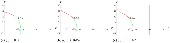
Figure 1. Spacetime diagram of the collapse of spherical dust for different values of $q_{*}$. The curve $T_s\left(r\right)$ denotes the trajectory of the surface of the star $r_s$ during the collapse. The static observer is at $r_o=10$.

By substituting the position of the surface of the star $r=r_s$, a maximum angular amplitude $\tilde{\alpha }=\pi /2$, and ${\epsilon }^2=1-2M\left(r_i\right)/r_i$ in the equality given by Equation (40), one obtains

$${\displaystyle \frac{r_m^3}{r_m-2M\left(r_m\right)}}={\displaystyle \frac{r_i{r}_s^2}{r_i-2M\left(r_i\right)}}.$$

(43)

As $r_s$ evolves during the collapse, the radius $r_m$ decreases up to the limiting value $r_{mp}$ given in (21). The value of $r_s$, for which $r_m=r_{mp}$ is reached, will be denoted as $r_s^{\left(2\right)}$ and marks the end of the second phase. Table 1 shows the values for the horizon radius $r_{+}$, the photosphere radius $r_{mp}$, and the radius for the end of the second phase $r_s^{\left(2\right)}$ for representative values of $q_{*}$.

Table 1. The Schwarzschild case corresponds to $q_{*}=0$, and the limit value of $q_{*}=1.0582$ corresponds to an extreme Hayward BH. As the value of $q_{*}$ increases, the other radii decrease.

${\mathbf{q}}_{*}$	${\mathbf{r}}_{+}$	${\mathbf{r}}_{\mathbf{mp}}$	${\mathbf{r}}_{\mathbf{s}}^{\left(2\right)}$
0.0	2.0	3.0	4.02492
0.8967	1.76981	2.8151	3.91263
1.0582	1.33985	2.6524	3.82057

The description of the shadow will depend on the relative position between the observer $r_o$ and the surface of the star. Thus, the static case will be divided into two cases: when the observer is always outside the star $r_o>r_i$ and when, for a moment, the observer is inside the star $r_s^{\left(2\right)}<r_o\le r_i$.

3.1. Static Observer Outside the Star

As in the previous case, the description of the shadow will be divided into three stages. In the first stage, before the collapse starts, the static observer describes a shadow with a constant angular size given by Equation (32), where we set $r_m=r_i$ and $r_i=r_o$, which correspond to the position of the observer.

$$sin\alpha =\sqrt{{\displaystyle \frac{r_i^3(r_o-2M\left(r_o\right))}{r_o^3(r_i-2M\left(r_i\right))}}}.$$

(44)

The beginning of the collapse marks the end of the first stage. By integrating Equation (24) from $r=r_i$ to $r=r_o$, we obtain $T_o^{\left(1\right)}$, that is, the time elapsed for a photon to travel from $r_m=r_i$ to $r_o$.

$$T_o^{\left(1\right)}={\int }_{r_i}^{r_o}\left[{\displaystyle \frac{\sqrt{2M\left(r\right)r}}{r-2M\left(r\right)}}+{\displaystyle \frac{\sqrt{r^5(r_i-2M\left(r_i\right))}}{(r-2M\left(r\right))\sqrt{(r_i-2M\left(r_i\right))r^3-(r-2M\left(r\right))r_i^3}}}\right]dr.$$

(45)

During the second stage, as the collapse is taking place, the shadow will be modeled based on the minimum radius through which the photons pass $r_m$. This minimum can be determined using the radius of the star’s surface $r_s$ for a given value of $r_i$, as given in Equation (43). We can use this expression for $r_m=r_m\left(r_s\right)$ in Equation (33) to obtain

$$\mathcal{R}(r,r_m\left(r_s\right))={\displaystyle \frac{r_i{r}_s^2(r-2M\left(r\right)}{r^3(r_i-2M\left(r_i\right))}}.$$

(46)

For the observer at $r=r_0$, the angular size of the shadow as a function of the surface of the star is given by means of Equation (32) as

$$sin\alpha =\sqrt{{\displaystyle \frac{r_i{r}_s^2(r_o-2M\left(r_o\right))}{r_o^3(r_i-2M\left(r_i\right))}}}.$$

(47)

From Equation (24), we can determine the time that photons take to travel from $r_s$ to the observer’s location at $r_o$.

$$T_o-T_s={\int }_{r_s}^{r_o}\left[{\displaystyle \frac{\sqrt{2M\left(r\right)r}}{r-2M\left(r\right)}}+{\displaystyle \frac{\sqrt{r^5(r_i-2M\left(r_i\right))}}{(r-2M\left(r\right))\sqrt{(r_i-2M\left(r_i\right))r^3-(r-2M\left(r\right))r_i{r}_s^2}}}\right]dr,$$

(48)

where $T_s$ is given by Equation (42). Therefore, with the star’s radius, one can find an implicit relation between the shadow angular size $\alpha$ and the time when the photons that leave the surface of the star reach the position of the static observer $T_o$.

The second stage ends when the minimum radius coincides with the limit value $r_m=r_{mp}$; we label the star’s radius at the end of this stage as $r_s=r_s^{\left(2\right)}$. The elapsed time during this stage is given by

$$\begin{array}{cc}\hfill T_o^{\left(2\right)}& =T_s\left(r_s^{\left(2\right)}\right)+{\int }_{r_s^{\left(2\right)}}^{r_o}{\displaystyle \frac{\sqrt{2M\left(r\right)r}}{r-2M\left(r\right)}}dr\hfill \\ \hfill & +{\int }_{r_s^{\left(2\right)}}^{r_o}{\displaystyle \frac{\sqrt{r^5(r_i-2M\left(r_i\right))}}{(r-2M\left(r\right))\sqrt{(r_i-2M\left(r_i\right))r^3-(r-2M\left(r\right))r_i{r}_s^{\left(2\right)2}}}}dr.\hfill \end{array}$$

(49)

The third stage is characterized because the minimum radius acquires a constant value $r_{\mathrm{m}}=r_{\mathrm{mp}}$. During this last stage, the photons coming from the source that reach the observer can graze, at most, the photosphere. Furthermore, during this stage, the angular size remains constant and is given by Equation (32) with $r=r_o$ and $r_m=r_{mp}$.

$$sin\alpha =\sqrt{{\displaystyle \frac{r_{mp}^3(r_o-2M\left(r_o\right))}{r_o^3(r_{mp}-2M\left(r_{mp}\right))}}}.$$

(50)

The first row of panels in Figure 2 displays the Schwarzschild case ($q*=0$) for the angular size of the shadow for a static observer. The left panel plots the angular size as a function of time for the observer (which coincides with the coordinate time). In the right panel, the observer’s sky is represented. In this representation, we consider that the black hole is on the left and the darker region represents the evolution of the shadow as a function of time. The gray-scale color code matches the value of $\alpha$. The darker the region, the higher the value of $\alpha$. The panels in the second and third rows represent the shadow angular size for spacetimes with representative values of the Hayward parameter. The extreme Hayward black hole corresponds to the value $q_m/M_0=1.05827$.

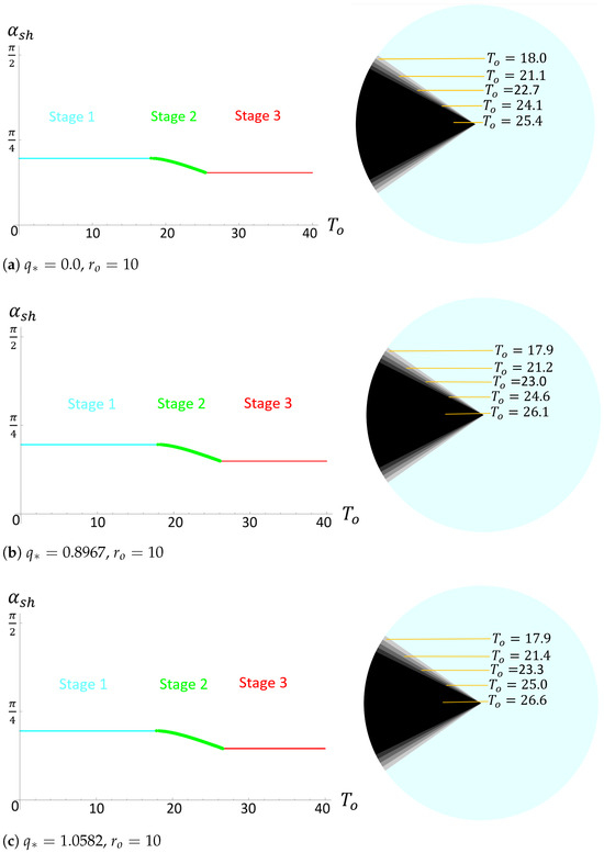
Figure 2. (Left) Angular size of the shadow ${\alpha }_{sh}$ as a function of time $T_o$ measured by the static observer at $r_o>r_i$ for different values of $q_{*}$. The color in the plot indicates the three different phases of the description. The first phase is the cyan part of the curve (Equation (44)), the second stage is the green part (Equation (47)), and the red color corresponds to the third and final phase (Equation (50)). (Right) Angular region of the shadow at different times. The black hole is to the left of the picture. The initial radius is $r_i=5$.

To summarize this scenario, when the static observer is located outside the initial radius of the star $r_i$, the determination of the shadow is divided into three stages: the first stage corresponds to photons that leave the source before the collapse begins and reach the observer; the second stage spans from the start of the collapse until the minimum radius at which photons can orbit ($r_m$) becomes equal to the value of the photosphere ($r_m=r_{mp}$); and the third stage covers the rest of the collapse. In this last stage, the radius of the star ($r_s$) continues to decrease but becomes irrelevant for the determination of the shadow since the minimum radius remains fixed at $r_{mp}$. For the static observer, the only change in the angular size of the shadow occurs during the second stage of the collapse when the minimum radius $r_m$ changes from $r_i$ to $r_{mp}$. This makes sense because the photons marking the edge of the shadow follow circular trajectories that depend on the size of the star until they reach that minimum limit. For the Schwarzschild case, for different initial observer radii, the closer the observer to the star, the larger the shadow angle. Additionally, the start of each stage begins earlier for smaller observer radii, as it takes less time for photons to travel from the star’s surface to the observer. For values of $q_{*}>0$, a higher value of the Hayward charge parameter leads to the second stage ending at a later $T_o$, as the photosphere’s radii value is smaller, causing photons to reach a smaller radius in their circular orbits. Since the second stage ends at a later time and $r_{mp}$ is smaller for small values of $q*$, this results in a smaller angular size in the last stage.

3.2. Static Observer Initially Located Inside the Star

In contrast to the previous case, the description of the shadow can only begin when the star’s radius is smaller than the observer’s radius since our model considers an opaque star. We also assume that $r_s^{\left(2\right)}<r_o$. The equations that define the angular size of the shadow correspond to Equations (47) and (48) in stage 2 and Equation (50) in stage 3.

Figure 3 shows the evolution of $\alpha$ over time $T_o$ measured by the static observer at $r_o$ for different values of $q_{*}$. For values of $q*$ near the extreme, the second stage lasts longer, and the value of $\alpha$ is smaller during the last stage for smaller values of $q*$.

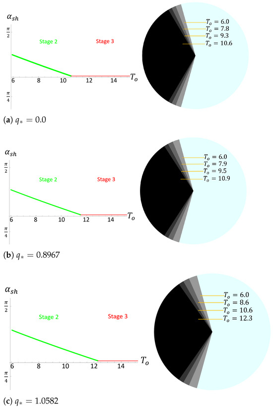
Figure 3. The shadow angular size ${\alpha }_{sh}$ as a function of $T_o$ determined by a static observer at $r_o=4.5$ for different values of $q_{*}$.

3.3. Free-Falling Observer

For a free-falling observer, the description of the shadow will also be divided into three stages. We shall consider that the initial radius of the star satisfies $r_i>r_{mp}$. We assume that the observer is initially located at radius $r_o^{*}$, large enough so that the observer is always outside the star. The time elapsed for the observer from the beginning of the collapse $T_o=0$ up to an arbitrary time $T_o$ (when the observer is located at $r_o$) is calculated by taking the quotient of Equations (10) and (11) and integrating

$$T_o={\int }_{r_o}^{r_o^{*}}{\displaystyle \frac{\epsilon \sqrt{r^3}-\sqrt{2M\left(r\right)r}\sqrt{{\epsilon }^{2}r-r+2M\left(r\right)}}{(r-2M\left(r\right))\sqrt{{\epsilon }^{2}r-r+2M\left(r\right)}}}dr$$

(51)

The value of the energy $\epsilon$ is determined by the initial velocity of the observer.

In Figure 4, we plot the trajectory $T_s=T_s\left(r\right)$ of the surface of the collapsing star alongside the trajectory of the falling observer $T_o=T_o\left(r\right)$ for some representative values of $q*$.

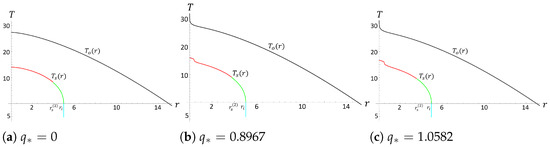
Figure 4. Spacetime diagram of the surface of the collapsing star and the trajectory of a free-falling observer for different values of $q_{*}$. The initial position of the observer is $r_o^{*}=15$.

For the first stage, which begins at an arbitrary (negative) time and ends when the collapse begins, the angular size shadow is determined using Equation (41) after taking $r=r_o$ and $r_m=r_i$.

$$sin\tilde{\alpha }={\displaystyle \frac{\sqrt{1-2M\left(r_o\right)/r_o}\sqrt{\mathcal{R}(r_o,r_i)}}{\epsilon +\sqrt{{\epsilon }^2-1+2M\left(r_o\right)/r_o}\sqrt{1-\mathcal{R}(r_o,r_i)}}},$$

(52)

where $\mathcal{R}$ is given in Equation (33). Thus, the angular size of the shadow will change according to the position of the observer.

In the second stage, where the radius of the surface of the star varies from $r_s=r_i$ to $r_s=r_s^{\left(2\right)}$, Equation (48) with $T_s$ given by Equation (42) and $T_o$ given by Equation (51) is as follows:

$$\begin{array}{c}\hfill {\int }_{r_o}^{r_o^{*}}{\displaystyle \frac{\epsilon \sqrt{r^3}-\sqrt{2M\left(r\right)r}\sqrt{{\epsilon }^{2}r-r+2M\left(r\right)}}{(r-2M\left(r\right))\sqrt{{\epsilon }^{2}r-r+2M\left(r\right)}}}dr={\int }_{r_s}^{r_i}{\displaystyle \frac{\sqrt{r^3}\sqrt{r_i-2M\left(r_i\right)}}{(r-2M\left(r\right))\sqrt{2M\left(r\right)r_i-2M\left(r_i\right)r}}}dr\\ \hfill +{\int }_{r_i}^{r_o}{\displaystyle \frac{\sqrt{2M\left(r\right)r}}{r-2M\left(r\right)}}dr+{\int }_{r_s}^{r_o}{\displaystyle \frac{\sqrt{r^5(r_i-2M\left(r_i\right))}}{(r-2M\left(r\right))\sqrt{(r_i-2M\left(r_i\right))r^3-(r-2M\left(r\right))r_i{r}_s^2}}}dr\end{array}$$

(53)

Hence, an equation relating the observer’s radius $r_o$ to the star’s radius $r_s$ is obtained.

Equation (32) with $r_m$ given by (41) and applied to the observer with $r=r_o$ gives the angular size as dependent on the value of $r_o$. By using both equations, the shadow’s angular size $\tilde{\alpha }$ can be modeled with respect to the observer’s radius $r_o$ as $r_s$ evolves.

The beginning of the third stage occurs when $r_s=r_s^{\left(2\right)}$ or in terms of the minimum radius $r_m=r_{mp}$. The angular size will then be given by Equation (41) in the following form:

$$sin\tilde{\alpha }={\displaystyle \frac{\sqrt{1-2M\left(r_o\right)/r_o}\sqrt{\mathcal{R}(r_o,r_{mp})}}{\epsilon \pm \sqrt{{\epsilon }^2-1+2M\left(r_o\right)/r_o}\sqrt{1-\mathcal{R}(r_o,r_{mp})}}}$$

(54)

Sign plus is used until the observer crosses $r_o=r_{mp}$, after which the negative sign must be used. This change in sign is due to the change in sign in Equation (23) that is induced when $r=r_{mp}$. This stage will last until the observer reaches $r_o=r_{+}$.

In the left panel of the first row in Figure 5, the angular size of the shadow is plotted as a function of the radius of the free-falling observer for the collapse, leading to a Schwarzschild black hole. In the plot, the three stages are shown in color. As the observer approaches the center, from the initial value $r_o^{*}=15$, the angular size increases monotonically up to a certain radius at which the size starts to decrease until a certain radius is reached, which characterizes the end of the second phase. After this radius is reached, the angular size increases again. In the right panel of the first row, the angular size is represented in the observer’s sky. The three stages are represented with the same color code as that detailed in the left column.

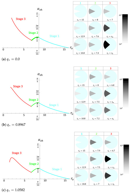
Figure 5. Plots of the spherical collapse of dust for different values of $q_{*}$. On the left side, the angular size ${\alpha }_{sh}$ is displayed as a function of the observer’s radius $r_o$; on the right side, the representation of the viewer’s sky is shown for different radii $r_o$. The corresponding stage of collapse is indicated at the top of the figure.

The magnitude of the angular size is represented in the gray color scale that spans from $\tilde{\alpha }={16}^{\circ }$ (white) to $\tilde{\alpha }={43}^{\circ }$ (black). From these figures, one can conclude that the effect on the shadow of the Hayward parameter $q*$ becomes more noticeable as the collapse progresses. Furthermore, the beginning of the third stage occurs at a smaller radius because the radius of the photosphere decreases with larger values of $q_{*}$. Therefore, the shadow has a smaller size at the end of the second stage. Additionally, at the end of the third stage, the shadow angle will be smaller if the Hayward parameter is large enough, and more importantly, it will have a local maximum. This behavior is related to the repulsive effect of the central core in the Hayward spacetime that dampens the gravitational contraction and is manifested in the shadow measured by the infalling observer.

The values for the maximum in the third stage for a free-falling observer are different depending on the value of the Hayward charge; for $q_{*}=0.0$, the maximum is at ${\alpha }_{sh}=0.734844$ for $r_s=2.0$; for $q_{*}=0.8967$, the maximum is at ${\alpha }_{sh}=0.675211$ for $r_s=1.76981$; and for $q_{*}=1.0582$, the maximum is at ${\alpha }_{sh}=0.600484$ for $r_s=1.90294$.

4. Final Remarks

In this work, we analyze the formation of the shadow of a regular Hayward black hole. The evolution of the angular size of the shadow during the collapse of a star in the regular Hayward spacetime is shown by analyzing the null geodesics. Our results show that, for a static observer outside the star, the behavior of the shadow is essentially divided into three stages. The first and third stages maintain a constant shadow angle since the minimum radius $r_m$ remains constant, obeying Equation (43). The change in the shadow’s angular size occurs in the second stage, where the star’s radius $r_s$, as well as the minimum radius $r_m$, decreases in time due to the collapse of the star. The end of the second stage and the beginning of the third depend on the value of the Hayward parameter $q_{*}$, since the radius of the photosphere depends on this. For a higher value of $q_{*}$, the second stage ends later, causing the shadow angle to reach a lower value. For observers between the photosphere radius and the initial radius of the star, the evolution of the shadow begins during the second stage once the star’s radius is smaller than that of the observer. For an observer between the horizon radius and the photosphere radius, the value of the shadow angle is constant and depends on the radius of the photon sphere. In the case of a radially falling observer, there are also three stages depending on the value of the minimum radius $r_m$. Unlike a static observer, this type of observer sees a change in the shadow angle at the end of the third stage. The relationship between the Hayward charge $q_{*}$ and the shadow angle is that, as the Hayward charge increases, the shadow angle will decrease close to the end of the third stage.

As a final remark, understanding the dynamical formation of black hole shadows in regular spacetimes is important not only for theoretical consistency but also for connecting models of singularity resolution to potential observational signatures. This study provides a perspective on the collapse evolution of regular black holes, revealing the effect of considering a regular metric to study the shadow of a collapsing star. By making a comparison with the Schwarzschild case, discussed, for example, in Ref. [7], our results show how the Hayward parameter modifies both the temporal formation and the final angular size of the shadow, offering a phenomenological window into possible deviations from classical general relativity. In particular, the relationship between the Hayward charge $q_{*}$ and the shadow angle is such that, as $q_{*}$ increases, the shadow angle decreases near the end of the third stage of collapse. This reduction in angular size arises from the effect of the Hayward charge near $r=0$, which prevents the formation of a central singularity during the collapse.

Additionally, beyond its theoretical interest, this model may also serve as a phenomenological tool to explore the possible observational signatures of regular black holes in scenarios where singularity resolution is expected, such as in quantum gravity-inspired corrections to general relativity. In particular, the influence of Hayward parameters on shadow evolution can be mapped to effective deviations that future observations might be sensitive to. Looking ahead, this framework can be extended to include rotation, accretion processes, or deviations motivated by other regular black hole models, providing a broader set of predictions that can be confronted with data from next-generation instruments aiming to resolve the dynamical aspects of black hole shadows.

References

- Akiyama, K.; Alberdi, A.; Alef, W.; Asada, K.; Azulay, R.; Baczko, A.K.; Ball, D.; Baloković, M.; Barrett, J.; Bintley, D.; et al. First M87 Event Horizon Telescope Results. IV. Imaging the Central Supermassive Black Hole. Astrophys. J. Lett. 2019, 875, L4. [Google Scholar] [CrossRef]
- Akiyama, K.; Alberdi, A.; Alef, W.; Asada, K.; Azulay, R.; Baczko, A.K.; Ball, D.; Baloković, M.; Barrett, J.; Bintley, D.; et al. First M87 Event Horizon Telescope Results. V. Physical Origin of the Asymmetric Ring. Astrophys. J. Lett. 2019, 875, L5. [Google Scholar] [CrossRef]
- Akiyama, K.; Alberdi, A.; Alef, W.; Algaba, J.C.; Anantua, R.; Asada, K.; Azulay, R.; Bach, U.; Baczko, A.K.; Ball, D.; et al. First Sagittarius A* Event Horizon Telescope Results. I. The Shadow of the Supermassive Black Hole in the Center of the Milky Way. Astrophys. J. Lett. 2022, 930, L12. [Google Scholar] [CrossRef]
- Akiyama, K.; Alberdi, A.; Alef, W.; Algaba, J.C.; Anantua, R.; Asada, K.; Azulay, R.; Bach, U.; Baczko, A.K.; Ball, D.; et al. First Sagittarius A* Event Horizon Telescope Results. II. EHT and Multiwavelength Observations, Data Processing, and Calibration. Astrophys. J. Lett. 2022, 930, L13. [Google Scholar] [CrossRef]
- Akiyama, K.; Alberdi, A.; Alef, W.; Algaba, J.C.; Anantua, R.; Asada, K.; Azulay, R.; Bach, U.; Baczko, A.K.; Ball, D.; et al. First Sagittarius A* Event Horizon Telescope Results. V. Testing Astrophysical Models of the Galactic Center Black Hole. Astrophys. J. Lett. 2022, 930, L16. [Google Scholar] [CrossRef]
- Vagnozzi, S.; Roy, R.; Tsai, Y.D.; Visinelli, L.; Afrin, M.; Allahyari, A.; Bambhaniya, P.; Dey, D.; Ghosh, S.G.; Joshi, P.S.; et al. Horizon-scale tests of gravity theories and fundamental physics from the Event Horizon Telescope image of Sagittarius A. Class. Quant. Grav. 2023, 40, 165007. [Google Scholar] [CrossRef]
- Schneider, S.; Perlick, V. The shadow of a collapsing dark star. Gen. Rel. Grav. 2018, 50, 58. [Google Scholar] [CrossRef]
- Oppenheimer, J.R.; Snyder, H. On Continued gravitational contraction. Phys. Rev. 1939, 56, 455–459. [Google Scholar] [CrossRef]
- Synge, J.L. The Escape of Photons from Gravitationally Intense Stars. Mon. Not. Roy. Astron. Soc. 1966, 131, 463–466. [Google Scholar] [CrossRef]
- Hayward, S.A. Formation and evaporation of regular black holes. Phys. Rev. Lett. 2006, 96, 31103. [Google Scholar] [CrossRef]
- Frolov, V.P. Notes on nonsingular models of black holes. Phys. Rev. D 2016, 94, 104056. [Google Scholar] [CrossRef]
- Flachi, A.; Lemos, J.P.S. Quasinormal modes of regular black holes. Phys. Rev. D 2013, 87, 24034. [Google Scholar] [CrossRef]
- Lin, K.; Li, J.; Yang, S. Quasinormal Modes of Hayward Regular Black Hole. Int. J. Theor. Phys. 2013, 52, 3771–3778. [Google Scholar] [CrossRef]
- Lopez, L.A.; Hinojosa, V. Quasinormal modes of Charged Regular Black Hole. Can. J. Phys. 2021, 99, 44–48. [Google Scholar] [CrossRef]
- Chiba, T.; Kimura, M. A note on geodesics in the Hayward metric. Prog. Theor. Exp. Phys. 2017, 2017, 43E01. [Google Scholar] [CrossRef]
- Wei, S.W.; Liu, Y.X.; Fu, C.E. Null Geodesics and Gravitational Lensing in a Nonsingular Spacetime. Adv. High Energy Phys. 2015, 2015, 454217. [Google Scholar] [CrossRef]
- Zhao, S.S.; Xie, Y. Strong deflection gravitational lensing by a modified Hayward black hole. Eur. Phys. J. C 2017, 77, 272. [Google Scholar] [CrossRef]
- Kumar, R.; Ghosh, S.G.; Wang, A. Shadow cast and deflection of light by charged rotating regular black holes. Phys. Rev. D 2019, 100, 124024. [Google Scholar] [CrossRef]
- Chowdhuri, A.; Ghosh, S.; Bhattacharyya, A. A review on analytical studies in Gravitational Lensing. Front. Phys. 2023, 11, 1113909. [Google Scholar] [CrossRef]
- Abbas, G.; Sabiullah, U. Geodesic Study of Regular Hayward Black Hole. Astrophys. Space Sci. 2014, 352, 769–774. [Google Scholar] [CrossRef]
- Bautista-Olvera, B.; Degollado, J.C.; German, G. Geodesic structure of a rotating regular black hole. Gen. Relativ. Gravit. 2023, 55, 66. [Google Scholar] [CrossRef]
- Debnath, U. Accretion and Evaporation of Modified Hayward Black Hole. Eur. Phys. J. C 2015, 75, 129. [Google Scholar] [CrossRef]
- Carballo-Rubio, R.; Di Filippo, F.; Liberati, S.; Pacilio, C.; Visser, M. On the viability of regular black holes. J. High Energy Phys. 2018, 7, 23. [Google Scholar] [CrossRef]
- Carballo-Rubio, R.; Di Filippo, F.; Liberati, S.; Visser, M. Phenomenological aspects of black holes beyond general relativity. Phys. Rev. D 2018, 98, 124009. [Google Scholar] [CrossRef]
- Mottola, E. Gravitational Vacuum Condensate Stars. In Regular Black Holes: Towards a New Paradigm of Gravitational Collapse; Bambi, C., Ed.; Springer: Berlin/Heidelberg, Germany, 2023; Chapter 8; pp. 283–352. [Google Scholar]
- Perez-Roman, I.; Bretón, N. The region interior to the event horizon of the Regular Hayward Black Hole. Gen. Relativ. Gravit. 2018, 50, 64. [Google Scholar] [CrossRef]
Disclaimer/Publisher’s Note: The statements, opinions and data contained in all publications are solely those of the individual author(s) and contributor(s) and not of MDPI and/or the editor(s). MDPI and/or the editor(s) disclaim responsibility for any injury to people or property resulting from any ideas, methods, instructions or products referred to in the content. |
© 2025 by the authors. Licensee MDPI, Basel, Switzerland. This article is an open access article distributed under the terms and conditions of the Creative Commons Attribution (CC BY) license (https://creativecommons.org/licenses/by/4.0/).