Abstract
Time-Sensitive Networking (TSN) provides end-to-end data transmission with extremely low delay and high reliability on the basis of Ethernet. It is suitable for time-sensitive applications and will be widely used in scenarios such as autonomous driving and industrial Internet. IEEE 802.1Qbv proposes a time-aware shaper mechanism, which enables switches to control the forwarding of traffic in port queues according to pre-defined Gate Control List (GCL). The length of the GCL is limited, and the previous method of scheduling cycle with a hyper period may result in a larger GCL. Based on Satisfiability Modulo Theories (SMT), we propose a TSN scheduling method for industrial scenarios and develops a series of scheduling constraints. Different from the previous scheduling methods, the method proposed in this paper adopts the base period cycle to update GCL regularly, which can effectively reduce the number of time slots in GCL and make the configuration of GCL simpler and more efficient. In addition, compared with the traditional hyper period method, the method proposed in this paper can calculate the scheduling results faster while ensuring low latency and reducing the runtime effectively.
1. Introduction
With the continuous popularization of the Industrial Internet of Things, increasingly intelligent terminal equipment and infrastructure have formed a super-intelligent system group, and the time-sensitive data (such as control data, fault monitoring data, etc.) generated by these systems must be transmitted within strict time and reliable regulations [1]. The original standard Ethernet IEEE802.3 [2] satisfies the bandwidth requirements of a wide range of application areas while maintaining scalability and cost-effectiveness, but it is not suitable for real-time and safety-critical applications. On the other hand, a variety of industrial Ethernet standards coexist on the market today, and the industrial Ethernet protocols used in different industrial equipment vary from equipment supplier, so the compatibility between various field bus is another big problem. Time-Sensitive Networking (TSN) just solves these challenges. TSN has the following key characteristics: it provides microsecond-level precise clock synchronization, such as 802.1AS [3], and provides multiple delay control mechanisms for time-sensitive traffic, such as 802.1Qbv [4]. With these features, TSN can provide QoS guarantees for the traffic it carries, and ensure real-time and deterministic data transmission. Due to the complexity of industrial communication and automation, more exploration is needed in the practical application of TSN. Researching and improving the performance of TSN is of great significance to the future development of industrial communication and automation control. The scheduling algorithm is a very important part of the network. The efficient work of the scheduling algorithm is closely related to the timely and reliably transmission of data. The problem of scheduling in TSN networks is a multi-objective combinatorial optimization problem, which has been proved to be NP-complete in previous work [5].
The scheduling in this article is based on the switch with 802.1Qbv function, and all devices in the network are time-synchronized. Figure 1 describes the simplified logic of the switch port with 802.1Qbv function. Each switch egress port has 8 priority queues, and the arriving flow enters different queues according to the priority. Each queue has a logical switch called GATE (G in Figure 1). When the value is 1, it means that the GATE of the queue is open, and the flow in the corresponding queue can be transmitted, and 0 means it is closed. Gate Control List (GCL) has a cycle period, so GATE will be opened/closed cyclically according to this period.
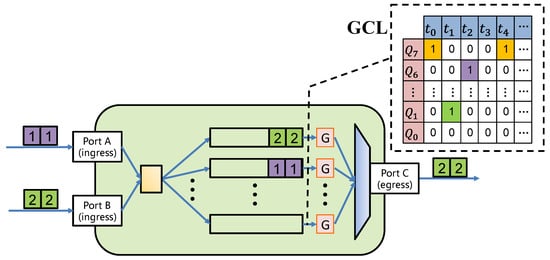
Figure 1.
Simplified view of an 802.1Qbv-capable switch.
This research focuses on the problem of Time-Triggered (TT) traffic scheduling in TSN, and proposes a network architecture that can dynamically manage TSN networks for industrial scenarios, TSN switch and the terminal system with time synchronization function can provide a real-time guarantee for the TT flow. Based on Satisfiability Modulo Theories (SMT), a TSN static scheduling algorithm for industrial scenarios is proposed, and a series of scheduling constraints are formulated. The previous researches on traffic scheduling based on 802.1Qbv have adopted hyper period for scheduling cycles. One of the biggest problems of hyper period is that the size of hyper period is very large, and an oversized hyper period results in a flow with a smaller period being scheduled multiple times per cycle, so many time slots are required for scheduling in each cycle. Larger length of GCL tables requires high-performance hardware support, and most current TSN switches cannot support larger GCLs. Different from the previous 802.1Qbv-based scheduling methods, the algorithm proposed in this paper uses the base period method to update GCL regularly, which can effectively reduce the number of time slot entries in the GCL and make the configuration of the GCL simpler and more efficient. Additionally, compared with the traditional ways of using hyper period, the scheduling method proposed in this paper can calculate the scheduling result faster while ensuring low latency and effectively reducing the runtime.
2. Related Work
Researches on Switched Ethernet has made progress in recent years, such as Avionics full-duplex Switched Etherne (AFDX) [6], TTEthernet [7], or TSN. Some articles have studied the time-predictability of the AFDX network, and analyzed some methods to realize the predictability of switched Ethernet [8,9]. However, the switches and end systems in the AFDX network are not synchronized with the global clock.
This paper only focuses on the transmission deterministic problem of TSN network. Many scholars have conducted different studies in this field. The work in [10] proposes an approach based on a Greedy Randomized Adaptive Search Program (GRASP) metaheuristic to solve the scheduling problem. The work in [11] formulates the scheduling constraints for IEEE 802.1Qbv using the first-order theory of arrays and solves the system’s satisfiability through the SMT solver. An SMT method is used to minimize the number of queues used for scheduling traffic, and to ensure that the remaining queues can be used for non-scheduled traffic in [12]. The work in [13] considers Audio-Video-Bridging (AVB) traffic when scheduling TT traffic, which uses Time-Aware Shaper (TAS) and Credit-Based-Shaper (CBS) scheduling mechanism, and combines routing and scheduling. The work in [14] proposes an iterative method based on SMT that combines routing and scheduling. The work in [15] based on SMT and 802.1Qbv presents a tool “TSNsched” to generate schedule. The above articles all use different scheduling algorithms, but they all use hyper period cycle (HPC) as the scheduling cycle. Therefore, in Section 5, we mainly compared the base period cycle (BPC) proposed in this paper as the scheduling cycle with HPC method.
For the scheduling of large-scale TSN, the work in [16] proposed a segmented approach, which splits the scheduling problem into smaller problems that can be solved independently. While maintaining the scheduling quality, it reduces the running time of the scheduler and can schedule a larger network in a shorter time. The work in [17] relaxes the scheduling rules, and divides the SMT problem into multiple Optimization Modulo Theories (OMT) problems, and reduces the runtime of the solvers to an acceptable level, and then a fast heuristic algorithm is proposed, which combines GCL and controls the time of packet injection to eliminate scheduling conflicts.
By using the logically centralized paradigm of Software-Defined Networks (SDN), given a set of predefined time-triggered flows, the work in [18] is the first to use Integer Linear Programming (ILP) to formulate the integration of routing and scheduling. Subsequently, the same author proposed incremental flow scheduling and routing algorithm in the article [19], which can dynamically add or delete flows by scheduling one at a time. However, the author did not use the time-aware shaper proposed in 802.1Qbv for gate control scheduling. The author proposed a concept of base period, and then divided the base period into multiple time slots, each time slot size is enough to make an MTU size data packets traverse the entire network, and each scheduled flow is allocated a time slot for scheduling. One problem with this is that the time slot reserved for each flow is too large, which causes a lot of bandwidth waste.
3. System Model
3.1. Overall Network Architecture
To meet the requirements of real-time reliability and flexible reconfiguration of the network for edge computing services in factories, this paper proposes an in-factory network architecture for industrial internet based on TSN technologies. The network controller is logically centralized, that is, it has a global view in switches, topology, and traffic, which is conducive to the realization of network control logic such as routing and scheduling. The architecture is divided into three layers, named the field layer, data layer, and application layer, as shown in Figure 2.
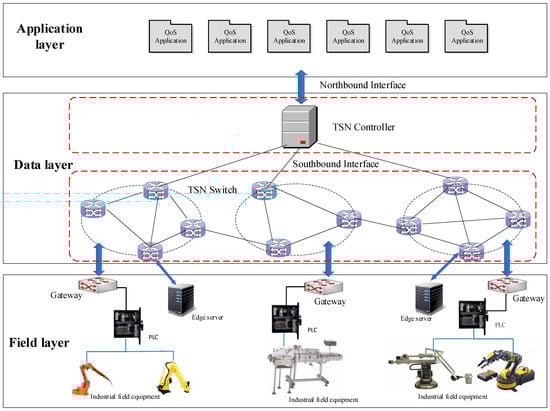
Figure 2.
Time-sensitive industrial architecture.
- (1)
- The field layer includes two parts: the traditional industrial production network and edge computing service equipment. The traditional industrial production network is composed of industrial field equipment, including industrial control machine, intelligent terminals, robots, programmable logic devices, numerical control machine tool, etc. Edge computing service equipment includes edge servers that process user requests and edge devices that seek for services.
- (2)
- The data layer is composed of TSN switches and TSN controllers. TSN switches are used for data forwarding. The controller is responsible for making the forwarding rules of the switch, calculating TSN switch traffic scheduling table and generating the bandwidth allocation strategies.
- (3)
- The application layer contains applications with different QoS requirements, and the applications in the application layer send requests to the TSN controller. Then, the TSN controller performs calculations, configures TSN scheduling and routing rules, and then sends them to the switch, and then to the industrial field layer.
The scheduling algorithm in this paper runs in the TSN controller for time-sensitive traffic scheduling on the data layer.
3.2. Terminologies and Notations
Figure 3 shows a simple TSN network architecture model. The architecture model including end systems, switches, and links. We model the topology of the TSN network as . The vertex set V refers to all devices in the network, including all end system set ES and all switch set SW. Therefore, . refers to the set of all data links in the network. The directed edge from to represents a unidirectional communication link from to . Therefore, the full-duplex link between the devices and is represented as two edges, defined as and . The notations used in this section are all described in Table A1.
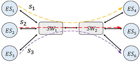
Figure 3.
Time-Sensitive Networking (TSN) network architecture model.
The entire article uses object-oriented notation to refer to specific attributes, e.g., represents the transmission rate of the link . We use to refer to the number of queues in the egress port connected to in .
We denote the set of flows in the network with , flow . A flow can be described by the tuple, denoting the period, the maximum allowed end-to-end latency (deadline) and the route of a flow, respectively. During the entire transmission process, the receiving end system must receive the message within . We use to represent the nodes passing through the routing path of , then . Since the research on routing has been done very well [20], we did not propose any routing algorithm. We stipulate that routing is generated on the basis of some existing algorithms.
We use to refer to the data packet sent by the flow in the -th period . A packet can be described by the tuple, denoting the packet size in bytes, the send time, the end-to-end delay and the transmission duration of a packet, respectively. The transmission duration of the packet on the port is related to packet size and transmission rate. Suppose that the size of a data packet is a maximum transmission unit MTU (1500 bytes) and the total overhead is 42 bytes, and the size of the entire packet is 1542 bytes. Then the transmission duration of packet sent to 1 Gbps link on the port is calculated in Equation (1).
The time period during which the queue gate in the egress port is opened and closed for each flow is called a time slot window, a time slot window can be described by the tuple, denoting the slot start time, the slot end time, and the queue ID of the slot, respectively. In port , the slot window opening time of flow is expressed as , and the closing time of slot window is expressed as . indicates in which queue the flow will be queued, so the upper limit of this value is the number of queues of the port . In this paper, the size of the time slot window will be taken as input and set to a fixed value. Users can define the size of the time slot by themselves.
The moment the packet is received by the receiver is denoted by . Then the time stamp calculation formula of the packet received by the receiver is as follows:
The end-to-end delay of the -th packet of flow is , which is calculated according to Equation (3).
Because the lines between nodes in industrial scenarios are short, the link propagation delay between nodes in most scenarios is negligible. In this paper, the link propagation delay is set to a fixed value of 1μs in the scheduling calculation.
3.3. Base Period
The GCLs of all egress ports constitute a definite timetable, and the switch forwards packets according to the timetable. Due to the periodicity of the flows, GCLs have a certain cycle time, after the first cycle, they will start from the beginning. In all previous traffic scheduling methods based on the 802.1Qbv, GCL is cycled according to the hyper period. One of the biggest problems of hyper period is that the size of hyper period is very large. Then in a scheduling cycle, a particularly large number of flows must be scheduled. So, the GCL is relatively large and there are many scheduling entries, which increases the complexity of scheduling. Naresh Ganesh Nayak proposed the concept of base period for the first time [18], this article defines that the transmission period of all flows is an integer multiple of the base period, and the base period is limited to be less than or equal to the lowest transmission period that a flow in the network may have. Inspired by Naresh Ganesh Nayak, our transmission scheduling was modeled as a cycle scheduling with a duration of base period, the GCL of each port cycled according to the base period. Therefore, in our scheduling algorithm, we use the idea of the base period to carry out scheduling analysis based on the 802.1Qbv scheduling mechanism. Additionally, we define the base period as the greatest common divisor (GCD) of all periods of the flows and is represented by symbol BP. The base period is divided into multiple time slots, and the number and size of time slots in each base period are the same. We set the opening/closing of the time slot in each base period to be the same, and GCL is configured according to the base period. All data packets of the same flow in the same switch egress port have the same priority and enter the same queue, so it is only necessary to determine the time slot of the first packet of each flow.
Flows with the same period (the period is ,) can use the same time slot for different base period. Flows with different periods and the flow with a period of BP cannot share the time slot, because flows of different periods use same time slots will cause time slot conflicts in some subsequent base period. Figure 4 describes an example of cycle scheduling using base period. There are three flows, the periods of and are both , and the period of is , and represent different time slot in a base period. and can use same time slot alternately in different base period, e.g., is scheduled in time slot in BP 1, and can be scheduled in time slot in BP 2. No flow in this example has the same period as , and is scheduled in slot , so slot cannot be used for and in any base period, which can be used if the period of other flows is the same as the period of . The opening/closing of the time slot in each base period is to be the same, so the GCL only needs to be configured in accordance with the gray part in Figure 4.
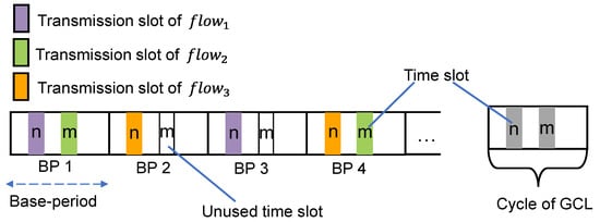
Figure 4.
Example of base period.
4. Scheduling Method Based on Satisfiability Modulus Theories
Satisfiability Modulo Theories (SMT) solver is a tool that can find the satisfiability or unsatisfiability of a set of constraints and are commonly used in verifiability problems [21], but the performance of SMT solvers has improved significantly in the past few years, making them applicable to more complex problems, such as scheduling problems. If the network is not schedulable for a given set of flows and constraints, the SMT solver will return unsatisfiability. The idea of using SMT solvers to search for distributed system scheduling was first proposed by Steiner [22]. The disadvantage of using SMT solvers is that, for large networks, it may take a long time to solve scheduling problems.
The entire workflow of the scheduling algorithm in this paper is described in Figure 5.
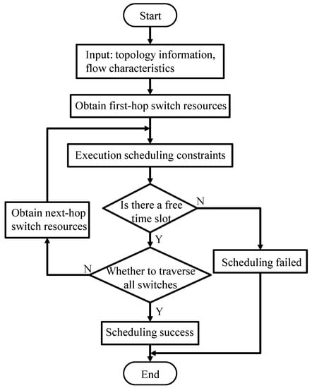
Figure 5.
Workflow of Satisfiability Modulo Theories (SMT) algorithm.
Scheduling Constraints
(1) Periodically send constraint. All packets must be sent periodically according to the period of the flow, which means that the flow will generate a data packet at every interval at the sending terminal, and the sending terminal must send the packet before the next packet is generated. The sending constraint of the sender is as follows:
The data sending port periodically sends packets, so after the sending time of the first packet of the flow is determined, the sending time of the subsequent generated packets is also determined.
(2) End-to-end delay constraint. The deadline of each flow is determined according to the specific requirements of the scenario, and the packet of flow must be fully received by the receiving terminal within the cut-off time . Define the constraint as follows:
;
The calculation of is shown in Equation (3). This constraint ensures that the end-to-end delay of flow cannot be greater than the deadline. We also added the clock synchronization accuracy δ to compensate for synchronization errors that may occur between the two nodes.
(3) Path order constraint. Packets must be transmitted along the routing path given in advance, and the time of the packet at the next node is greater than the time of the previous node.
Here, represents the previous node of in the routing path of flow , and these nodes have been stored in advance in the order of routing nodes, and 1 is the link propagation delay.
(4) Queuing constraint. In order to prevent the nondeterministic caused by different packets queuing in the egress port, we have formulated corresponding queue constraint. This constraint is mainly for the case that packets transmitted from different nodes are forwarded to the same node at the same egress port, that is, the case where there are the same links in different routing paths.
Figure 6a illustrates the nondeterministic queuing of flow. Two flows arrive at the same switch from different devices almost simultaneously and enter the same queue. Due to some factors, such as inaccurate clock synchronization between individual devices and frame loss, nondeterministic may appear when the flow is queued. We have two solutions for this situation. The first is shown in Figure 6b. Two flows are allocated to the same queue, and the opening time of the queue Gate of the previous node is controlled. Only after the current flow is forwarded, the latter flow can enter the queue, which is achieved the time isolation between different flows and avoids interleaving. The second method is shown in Figure 6c, allotting two flows to different queues, so that even if the arrival time of two flows are close, the flow can be isolated and conflicts can be avoided.
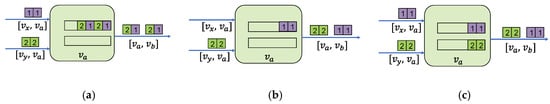
Figure 6.
Example of flow queuing on port. (a) Nondeterministic queuing. (b) Time isolation. (c) Assign to different queues.
For flows arriving from the same device, the first constraint (periodically send constraint) will ensure that the data packets of the flow will not overlap in the time domain. Assuming that the data packets and generated by flows and are forwarded to the device via device , and the flow reaches from the device via the link [], and the flow reaches from the device via the link []. The constraint is as follows:
This constraint indicates that for packets assigned to the same queue, the current packet can enter the queue only after the previous packet is forwarded, or two different packets are assigned to different queues.
(5) Link congestion constraint. This constraint ensures that only one packet can enter the link at a time on each port, that is, packets entering the same link cannot overlap in the time domain.
This is achieved by sequential transmission of packets from the same flow. For packets from different flows, if they enter the same queue, constraint (4) can ensure that packets entering the same queue will not conflicts in the time domain when they are forwarded, if they enter different queues, constraint needs to be formulated to ensure that packets from different queues in the same port will not collide when they enter the link. Define constraints as follows:
(6) Queue usage constraint. The number of queues allocated to time-critical flows cannot be greater than the number of port queues. Define λ as the number of queues that allocated to scheduled traffic by the port. All packets of the same flow enter the same queue. The constraints are as follows:
(7) Time slot window size constraint. We will give a slot window size as input, so that we can determine the time slot size according to the basic information of the network. This value is set as the time for an MTU-sized packet to pass through the switch port, so that all packets of all sizes can pass through the port. The constraint is as follows:
This constraint can be used to optimize the bandwidth used for scheduling traffic. If there is no limit on the size of the time slot window, it is likely that a time slot window will occupy all the time in a base period, so that there is no guarantee that there is remaining time to transmit the best effort traffic. The user can decide by himself whether the constraint is required according to the actual network scenario.
In addition, the time slot window cannot span the base period, so we limit the start time and end time of the window to be in the same base period, and the constraints are as follows:
(8) Time slot window transmission constraint. Packets must be transmitted during the corresponding time slot window, so the start time of the time slot window of the packet on the port cannot be greater than the time when the packet starts transmission, and the end time of window cannot be less than the time when the packet ends transmission.
This constraint ensures that there is enough time slot window to transmit packets, thus avoids the situation where the time slot window is smaller than the packet transmission time and the transmission is interrupted.
(9) Time slot window allocation constraint. For flows with the same period in the same port, e.g., the period of two flows , the same time slot in different base period can be allocated. Since the scheduling entries of the same time slot in GCL have the same setting, the data packets allocated to the same time slot should also be allocated to the same queue.
The same time slot cannot be shared between flows with different periods and flows with a period equal to the BP. The constraints are as follows:
The value of in the formula is the start time of the slot window allocated to the flow in the first base period. Once the time slot of flow is determined, the time period corresponding to the time slot in all BP is reserved exclusively, and the flow cannot be used any more. Therefore, the Equation (19) restricts the flow to only select the remaining unreserved time slots for scheduling in each BP.
(10) Period scheduling constraints. The scheduling time of each flow at the port is scheduled periodically according to the period . The time when the flow arrives at the port is represented by , and the slot window must be within the corresponding scheduling period. In other words, after the packet of the flow with period arrives at port , only the time slot window within after the arrival time can be selected for scheduling. After the time slot of the first packet is determined, the time slots of other packets in the same flow are also determined. Then there are the following constraints:
All packets of the same flow are scheduled in the same time slot of different BP, and the time interval is . Once the corresponding time slot is determined for the first data packet of the flow, the time slot for subsequent data packets of the flow is also determined.
5. Evaluation
There are many different program implementations of SMT solver. In this paper, we use the most widely used Z3 solver [19] to encode the SMT problem. The solution process of this paper based on the SMT scheduling algorithm is as follows:
- (1)
- Use the SMT method to construct TSN traffic scheduling problem constraints.
- (2)
- According to the proposed constraints, Z3 is used for encoding.
- (3)
- Construct network topology and flow information.
- (4)
- A feasible solution that satisfies the constraints is calculated through Z3.
- (5)
- Until the time slots of all flows are determined, the scheduling ends.
Scheduling input: We take the network topology, flow information (including period, routing, size of packets, deadline) and the maximum time slot window as input.
Scheduling output: The sending time of the flow at each node; The arrival time of each node in the flow path; The opening and closing time of the slot window of the of each switch egress port; The end-to-end delay of each flow; The time required to generate the schedule.
The scheduling problem was solved by our code on an Intel(R) Core (TM) i7-7700 CPU @ 2.50 GHz machine with 8 GB memory. We used the Z3 v4.8.8 solver (64-bit) [23], which, in addition to the normal SMT function, also has an algorithm for solving linear optimization goals [24]. We use TSNsched [15] to randomly generate network topology, and user-defined network topology is created with JAVA. Our program and algorithm use JAVA in the linux environment, and the data processing uses MATLAB. For convenience, we choose the timeline granularity as 1 μs, and the communication speed of all links is 1 Gbit/s.
We evaluated the time required to generate the schedule (Use “runtime” instead in the following articles.), the average end-to-end delay of all flows in each test case, and the worst-case end-to-end delay (Refers to the largest end-to-end delay in this test case.). Additionally, the BPC scheduling cycle method proposed in this paper is compared with the previous HPC scheduling cycle method.
5.1. User-Defined Network
This article has created two network topologies as shown in Figure 7, which are divided into small and medium-sized networks according to the size of the network topology, as shown in Figure 7a,b, respectively.
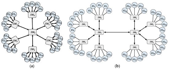
Figure 7.
User-defined network topology example. (a) Small network topologies. (b) Medium network topologies.
The small network consists of 7 switches and 30 terminal systems, all the scheduling flow will be forwarded by the , so when the number of flows is large, there will be flow conflicts and bandwidth contention in . Using the algorithm of this paper to conduct a scheduling test, we can schedule the number of flows with a packet size of 1500 bytes is 47 (all the flows forwarded by ). When the number of flows is increased to 48, the program did not return a result within 50 h.
The medium network consists of 10 switches and 40 terminal systems. All of our tests, the sender is to , and the receiver is to , so all flows will be forwarded to via . At the port , multiple flows will compete for network bandwidth, if not for scheduling, which may cause excessive flow delay or packet loss. We set up multiple test cases for the number of flows from low to high, and performed scheduling tests in turn to test the scheduling quality of the scheduling algorithm in the worst case. The worst case of scheduling, that is, there is only scheduled traffic in the network, and there is no best-effort traffic and all flows are forwarded to through , we can schedule the number of flows with a packet size of 1500 bytes is 28.
We first set up all flow periods in the test cases to be the same, then set up the flow of different periods in the test cases, and created more than 350 test cases for evaluation.
5.1.1. Flows Have the Same Period
Figure 8 describes the results of the test in the small network, increasing the scheduling flows in turn, and analyzes the changes in runtime and delay when the flow period is set to 300 μs, 500 μs, 1000 μs, and 2000 μs. Each time the period is changed, the number of flows increases from 2 to 47, the packet size is set to 1500 bytes, and the deadline is set to 1000 μs. There are 184 test cases in total.
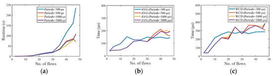
Figure 8.
Small network scheduling results. The flows in each test case have the same period. (a) Runtime. (b) Average end-to-end delay. (c) Worst-case end-to-end delay.
Figure 8a shows the relationship between the runtime and the number of flows. As the number of flows increases, the runtime gradually increases. When the period is set to 500 μs, 1000 μs, and 2000 μs, the difference between the runtime is not big, but it increases significantly when the period is set to be very small (e.g., 300 μs). Figure 8b,c shows that the average end-to-end delay (AVG) of all flows and worst-case end-to end delay (WCD) are kept within a small range, meeting the deadline of 1000 μs.
Then the test is carried out in the medium-sized network, and three groups of test cases are set up. The information of test cases is shown in Table 1. The transmission period of the flow in each test group is the same. The scheduling results are shown in Figure 9.

Table 1.
Test cases. Each group has 7 test cases according to the number of flows.
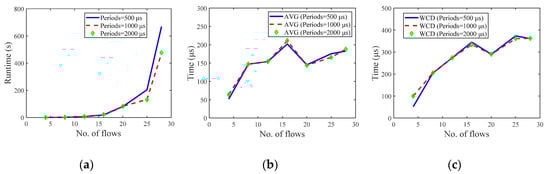
Figure 9.
Medium network scheduling results. The flows in each test case have the same period. (a) Runtime. (b) Average end-to-end delay. (c) Worst-case end-to-end delay.
Figure 9a shows the relationship between the scheduling runtime and the number of flows. With the number of flows increases, the runtime gradually increases. When the number of flows is small, there is almost no difference in the runtime of the three groups of test cases, but with the increase of the number of flows, the runtime of the test cases with 500 μs period increases faster than the other two groups. Figure 9b,c shows the AVG and WCD variation. The WCD increases with the number of flows, but all of them are within 400 μs, meeting the deadline of 1000 μs. The changes of runtime and latency of the two groups of test cases with periods of 1000 μs and 2000 μs are basically the same.
5.1.2. Flows have Different Period
The period of the flow in all test cases is arbitrarily selected from {500 μs, 1000 μs, 2000 μs, 4000 μs}, and the size of all data packets is 1500 bytes, and the deadline is set to 1000 μs.
First, the scheduling test was carried out in the small network. After the flow period is set, BP is calculated and the test cases with the same BP are in the same group. Additionally, 3 groups were set up, each group contains multiple test cases. The changes of runtime and latency are compared when the BP size is 500 μs, 1000 μs, and 2000 μs. The test results are shown in Figure 10.
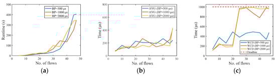
Figure 10.
Small network test results. The period of the flow in all test cases is arbitrarily selected from {500 μs, 1000 μs, 2000 μs, 4000 μs}. (a) Runtime. (b) Average end-to-end delay. (c) Worst-case end-to-end delay.
Figure 10a shows that when the number of flows is the same, the size of the BP will affect the running time, but the difference between the three groups of tests is not large. As the number of flows increases, the test case with a smaller BP increases faster. Figure 10b,c shows the AVG and WCD variation. All the AVG is lower than 500 μs. In the group with a BP of 500 μs, the WCD is smaller, but when the number of flows increases, the WCD in the test cases with a BP of 1000 μs and 2000 μs is larger, but both are lower than 1000 μs, meeting the deadline of 1000 μs.
Then it was tested in the medium network. The changes of runtime and latency are compared when the BP size is 500 μs, 1000 μs, and 2000 μs. Figure 11 shows the running results. The runtime increases with the increase of the number of flows. When the same number of flows is scheduled, the difference in the runtime when the BP is 1000 μs and 2000 μs respectively is small. As the number of flows increases, the runtime is smaller when the BP is 500 μs. Figure 11b,c shows the AVG and WCD variation. AVG and WCD in all test cases are lower than 1000 μs, meeting the deadline of 1000 μs.
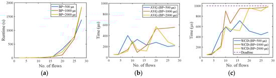
Figure 11.
Medium network test results. The period of the flow in all test cases is arbitrarily selected from {500 μs, 1000 μs, 2000 μs, 4000 μs}. (a) Runtime. (b) Average end-to-end delay. (c) Worst-case end-to-end delay.
5.2. Randomly Generated Network Using Network Tools
In this section, we evaluate the traffic scheduling in the randomly generated network. We use TSNsched [15] to generate multiple test cases with different network topology sizes and the number of flows to evaluate the scheduling quality of our algorithm.
Firstly, considering the influence of the number of flows on the runtime, we randomly generated 75 test cases in a large network system (20 switches and 100 terminals) with a hop count of 3, and 3 groups were set up, and flow period is 500 μs, 1000 μs, and 2000 μs, respectively. Each time the period is changed, the number of flows increases from 5 to 100, the packet size is set to 1500 bytes, and the deadline is set to 1000 μs. The scheduling results are shown in Figure 12a. The runtime increases with the increase of the number of flows. When the number of flows is small, there is basically no difference in the runtime between different periods. When the number of flows is large, the smaller the period is, and the longer the running time is.
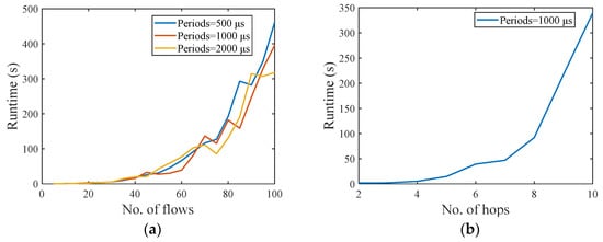
Figure 12.
Randomly generated network. The size of all data packets is 1500 bytes. (a) The impact of the number of scheduling flows on runtime. (b) Impact of flow hop count on runtime.
Then, considering the impact of the number of hops of the flow on the scheduling runtime, 9 test cases with a flow number of 20 and a hop number of 2–10 were randomly generated in the above-mentioned large network system. The scheduling results are shown in Figure 12b. The number of hops has a great impact on the scheduling runtime. However, the overall scheduling quality of our scheduling algorithm is better. When the hop count is 10, the runtime of scheduling 20 flows is 339.72 s.
5.3. Comparison of Base Period and Hyper Period
In the small network, taking 5 flows as an example, we compared our BPC method with the HPC method. The basic idea is to use flows of different periods to understand the performance difference between the two method. The sending terminals of the 5 flows are , , , , and , and the receiving terminals are , , , , and . A total of 8 test cases were set, the information about the sending period, base period size, and hyper period size of each test case are shown in Table 2.
Table 2.
Test cases information in the small network. Sending period of terminals, base period size (GCD), and hyper period size (LCM) per test-case, and the unit is μs.
Figure 13 shows the comparison results of the two methods used in test cases 1 to 8 in terms of scheduling runtime, where all results meet the delay requirement. The results show that when the periods of the flows are the same, the scheduling runtime of the two methods is similar. However, when scheduling different period flows, BPC method is obviously superior to the HPC method, and BPC can calculate the results at a faster speed.
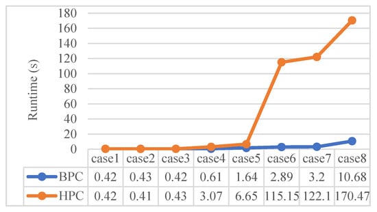
Figure 13.
Comparison of the runtime of the two methods in a small network.
Then, in the medium network, the BPC method is compared with the HPC method, and the runtime of the same flow period and different flow period is compared. Figure 14a shows the running results when all flow periods were the same. A total of 9 test cases were set, the number of flows was set to 12, and the packet size is 1500 bytes, and the sending period increases from 300 μs to 3000 μs. It can be seen from the results that when all flows have the same period, there is no significant difference between the two methods. Figure 14b shows the running results of different flow periods. The number of flows was set to 8, and the packet size is 1500 bytes. The sending terminals of the 8 flows are , , , , , , , and , a total of 20 test cases were set, the information about the sending period, base period size, and hyper period size of each test case are shown in Table A2.
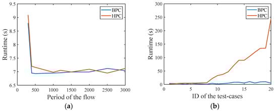
Figure 14.
Comparison of the runtime of the two methods in the medium network. (a) The period of the flow is the same. (b) The period of the flow is different.
It can be seen from the results that the BPC method has a lower runtime in these 20 test cases, which is obviously better than the HPC method. Additionally, for 60% of the test cases, the BPC method is significantly better than HPC method, especially for case20.
Finally, the number of GCL slot entries required by BPC method and HPC method for scheduling is compared, and the results are shown in Figure 15. Figure 15a shows the number of GCL slot entries required on ports [,] when the test cases in Table 2 is scheduled. Figure 15b shows the number of GCL slot entries required on ports [,] when the test cases in Table A1 is scheduled. The results shown in the figure reflect the worst-case scheduling (one slot per flow per BP, one slot per packet per HP). It can be seen that the BPC method we proposed can significantly reduce the number of time slot entries in GCL.
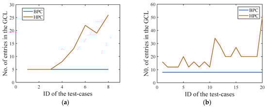
Figure 15.
Comparison of the number of Gate Control List (GCL) time slot entries. (a) Result of port [, ]. (b) Result of port [, ].
6. Conclusions and Next Work
This paper studies the traffic scheduling problem in Time-Sensitive Networking. A network architecture that can dynamically manage TSN networks applied to the industrial networks is proposed. On the basis of 802.1Qbv and clock synchronization, a scheduling algorithm based on base period is proposed by using the Satisfiability Model Theory, which can greatly reduce the size of GCL and simplify the configuration of switch ports. A series of scheduling constraints were formulated, and the scheduling quality of our method was evaluated in a variety of network topologies. The results show that the algorithm can quickly calculate the scheduling results, with a relatively low end-to-end delay, and compared with the previous scheduling of using hyper period, the results show that our scheduling algorithm can calculate the scheduling results faster.
We are currently conducting research on dynamic scheduling algorithms, and intend to implement dynamic incremental scheduling based on our static scheduling, mainly for scenarios where the scheduled traffic in the network may change.
Author Contributions
Conceptualization, Q.L. and X.J.; methodology, Q.L., D.L. and X.J.; software, Q.L. and Q.W.; validation, Q.L., D.L., X.J., Q.W. and P.Z.; investigation, Q.L.; resources, D.L. and P.Z.; data curation, Q.L.; writing—original draft preparation, Q.L.; writing—review and editing, Q.L., D.L., X.J., Q.W. and P.Z.; supervision, D.L.; project administration, D.L. and P.Z.; funding acquisition, D.L. and P.Z. All authors have read and agreed to the published version of the manuscript.
Funding
This research was funded by National Key R&D Program of China (2018YFB1702000), and was funded by Industrial Internet Innovation and Development Project (Project of Basis Standard and Experimental Verification for Industrial Software Defined Networking), and in part by Ningbo Science and Technology project (2018B10089).
Conflicts of Interest
The authors declare no conflict of interest.
Appendix A
Table A1.
Notations are used in this paper.
Table A1.
Notations are used in this paper.
| Notation | Description |
|---|---|
| V | Vertex set |
| E | Link set |
| SW | Switch set |
| ES | End system set |
| S | Flow set |
| A single network node | |
| A single flow | |
| Transmission rate of the link | |
| Number of queues in egress port | |
| Routing path of flow | |
| Deadline of flow | |
| Period of flow | |
| Packet sent by the flow in the -th period | |
| End-to-end delay of packet | |
| ρ | Packet size |
| Transmission duration of packet in port | |
| Send time of packet in port | |
| Time slot start time of packet in port | |
| Time slot end time of packet in port | |
| Time when packet arrives at port | |
| Q | The ID of the queue used by flow |
| λ | Number of queues that allocated to scheduled traffic |
| Moment the packet is received by the receiver | |
| δ | Clock synchronization accuracy |
Appendix B
Table A2.
Test cases information in the medium network. Sending periodicity of terminals, base period size (GCD) and hyper period size (LCM) per use-case, and the unit is μs.
Table A2.
Test cases information in the medium network. Sending periodicity of terminals, base period size (GCD) and hyper period size (LCM) per use-case, and the unit is μs.
| GCD | LCM | |||||||||
|---|---|---|---|---|---|---|---|---|---|---|
| case 1 | 1200 | 1200 | 1200 | 1200 | 3600 | 3600 | 3600 | 3600 | 1200 | 3600 |
| case 2 | 1000 | 1000 | 1000 | 1000 | 500 | 500 | 500 | 500 | 500 | 1000 |
| case 3 | 1500 | 1500 | 1500 | 1500 | 3000 | 3000 | 3000 | 3000 | 1500 | 3000 |
| case 4 | 2000 | 2000 | 2000 | 2000 | 4000 | 4000 | 4000 | 4000 | 2000 | 4000 |
| case 5 | 1800 | 1800 | 1800 | 1800 | 2700 | 2700 | 2700 | 2700 | 900 | 5400 |
| case 6 | 2500 | 2500 | 2500 | 2500 | 5000 | 5000 | 5000 | 5000 | 2500 | 5000 |
| case 7 | 300 | 300 | 300 | 300 | 900 | 900 | 900 | 900 | 300 | 900 |
| case 8 | 1000 | 1000 | 1000 | 1000 | 2000 | 2000 | 2000 | 2000 | 1000 | 2000 |
| case 9 | 1200 | 3600 | 1200 | 3600 | 1200 | 1200 | 3600 | 3600 | 1200 | 3600 |
| case 10 | 600 | 300 | 300 | 300 | 600 | 600 | 600 | 300 | 300 | 600 |
| case 11 | 2000 | 2000 | 2000 | 2000 | 4000 | 4000 | 6000 | 6000 | 2000 | 12000 |
| case 12 | 300 | 300 | 600 | 600 | 600 | 600 | 900 | 900 | 300 | 900 |
| case 13 | 1200 | 1800 | 1200 | 1800 | 1200 | 1200 | 1800 | 1800 | 600 | 3600 |
| case 14 | 1500 | 1000 | 1500 | 1000 | 1000 | 1000 | 1500 | 1500 | 500 | 3000 |
| case 15 | 500 | 500 | 1500 | 1500 | 1500 | 1000 | 1000 | 1000 | 500 | 3000 |
| case 16 | 5000 | 7500 | 5000 | 7500 | 5000 | 5000 | 7500 | 7500 | 2500 | 15000 |
| case 17 | 3000 | 4500 | 3000 | 4500 | 3000 | 3000 | 4500 | 4500 | 1500 | 9000 |
| case 18 | 2000 | 2000 | 2000 | 3000 | 3000 | 2000 | 3000 | 3000 | 1000 | 6000 |
| case 19 | 1800 | 2700 | 1800 | 2700 | 1800 | 1800 | 2700 | 2700 | 900 | 5400 |
| case 20 | 1000 | 1000 | 2000 | 2000 | 3000 | 3000 | 4000 | 4000 | 1000 | 12000 |
References
- Nasrallah, A.; Thyagaturu, A.S.; Alharbi, Z.; Wang, C.; Shao, X.; Reisslein, M.; ElBakoury, H. Ultra-low latency (ULL) networks: The IEEE TSN and IETF DetNet standards and related 5G Ull research. IEEE Commun. Surv. Tutor. 2019, 21, 88–145. [Google Scholar] [CrossRef]
- 802.3-2015-IEEE Standard for Ethernet. Available online: https://ieeexplore.ieee.org/document/7428776 (accessed on 4 October 2020).
- Institute of Electrical and Electronics Engineers, Inc, “802.1AS-Rev: Timing and Synchronization for Time-Sensitive Applications”. Available online: http://www.ieee802.org/1/pages/802.1AS-rev.html (accessed on 3 September 2020).
- Institute of Electrical and Electronics Engineers, Inc, “802.1Qbv: Enhancements for Scheduled Traffic”. Available online: https://standards.ieee.org/standard/802_1Qbv-2015.html (accessed on 20 August 2020).
- Lo Bello, L.; Steiner, W. A Perspective on IEEE Time-Sensitive Networking for Industrial Communication and Automation Systems. Proc. IEEE 2019, 107, 1094–1120. [Google Scholar] [CrossRef]
- Aeronautical Radio, Inc. ARINC 664P7: Aircraft Data Network, Part 7, Avionics Full-DupleX Switched Ethernet Network (AFDX). 2009. Available online: https://standards.globalspec.com/std/1283307/arinc-664-p7 (accessed on 4 October 2020).
- SAE. AS6802: Time-Triggered Ethernet; SAE International: Warrendale, PA, USA, 2011. [Google Scholar]
- Vila-Carbo, J.; Tur-Massanet, J.; Hernandez-Orallo, E. Analysis of Switched Ethernet for Real-Time Transmission. Tech. Fact. Autom. 2010, 221–239. [Google Scholar] [CrossRef]
- Vila-Carbó, J.; Tur-Masanet, J.; Hernández-Orallo, E. An evaluation of switched Ethernet and Linux Traffic Control for real-time transmission. In Proceedings of the 13th IEEE International Conference on Emerging Technologies and Factory Automation, Hamburg, Germany, 15–18 September 2008; pp. 400–407. [Google Scholar]
- Gavrilut, V.; Pop, P. Scheduling in time sensitive networks (TSN) for mixed-criticality industrial applications. In Proceedings of the IEEE International Workshop on Factory Communication Systems (WFCS), Imperia, Italy, 13–15 June 2018; pp. 1–4. [Google Scholar]
- Serna Oliver, R.; Craciunas, S.S.; Steiner, W. IEEE 802.1Qbv gate control list synthesis using array theory encoding. In Proceedings of the IEEE Real-Time and Embedded Technology and Applications Symposium (RTAS), Porto, Portugal, 11–13 April 2018; pp. 13–24. [Google Scholar]
- Craciunas, S.S.; Serna, R.; Martin, O.; Steiner, C.W. Scheduling real-time communication in IEEE 802.1Qbv time sensitive networks. In Proceedings of the 24th International Conference on Real-Time Networks and Systems, New York, NY, USA, 19–21 October 2016; pp. 183–192. [Google Scholar]
- Gavrilut, V.; Zhao, L.; Raagaard, M.L.; Pop, P. AVB-Aware routing and scheduling of time-triggered traffic for TSN. IEEE Access 2018, 6, 75229–75243. [Google Scholar] [CrossRef]
- Mahfouzi, R.; Aminifar, A.; Samii, S.; Rezine, A.; Eles, P.; Peng, Z. Stability-aware integrated routing and scheduling for control applications in Ethernet networks. In Proceedings of the 2018 Design, Automation and Test in Europe Conference and Exhibition (DATE), Dresden, Germany, 19–23 March 2018; pp. 682–687. [Google Scholar]
- Santos, A.C.T.D.; Schneider, B.; Nigam, V. TSNSCHED: Automated schedule generation for time sensitive networking. In Proceedings of the 19th Conference on Formal Methods in Computer-Aided Design (FMCAD), San Jose, CA, USA, 22–25 October 2019; pp. 69–77. [Google Scholar]
- Pozo, F.; Rodriguez-Navas, G.; Hansson, H. Methods for large-scale time-triggered network scheduling. Electronics 2019, 8, 738. [Google Scholar] [CrossRef]
- Jin, X.; Xia, C.; Guan, N.; Xu, C.; Li, D.; Yin, Y.; Zeng, P. Real-time scheduling of massive data in time sensitive networks with a limited number of schedule entries. IEEE Access 2020, 8, 6751–6767. [Google Scholar] [CrossRef]
- Nayak, N.G.; Dürr, F.; Rothermel, K. Time-sensitive Software-defined Network (TSSDN) for Real-time Applications. In Proceedings of the 24th International Conference on Real-Time Networks and Systems, New York, NY, USA, 19–21 October 2016; pp. 193–202. [Google Scholar]
- Nayak, N.G.; Durr, F.; Rothermel, K. Incremental flow scheduling and routing in time-sensitive software-defined networks. IEEE Trans. Ind. Inform. 2018, 14, 2066–2075. [Google Scholar] [CrossRef]
- Nayak, N.G.; Dürr, F.; Rothermel, K. Routing algorithms for IEEE802.1qbv networks. ACM SIGBED Rev. 2018, 15, 13–18. [Google Scholar] [CrossRef]
- Katz, G.; Barrett, C.; Dill, D.L.; Julian, K.; Kochenderfer, M.J. Reluplex: An efficient smt solver for verifying deep neural networks. In Proceedings of the Computer Aided Verification Conference (CAV), Heidelberg, Germany, 24–28 July 2017. [Google Scholar]
- Steiner, W. An evaluation of SMT-based schedule synthesis for time-triggered multi-hop networks. In Proceedings of the 31st IEEE Real-Time Systems Symposium, San Diego, CA, USA, 30 November–3 December 2010; pp. 375–384. [Google Scholar]
- Z3Prover. The z3 Theorem Prover. Available online: https://github.com/Z3Prover/z3 (accessed on 4 October 2020).
- Bjørner, N.; Phan, A.D.; Fleckenstein, L. νZ—An Optimizing SMT Solver. In Tools and Algorithms for the Construction and Analysis of Systems; Baier, C., Tinelli, C., Eds.; TACAS: Iloilo, Philippines, 2015; pp. 194–199. [Google Scholar]
Publisher’s Note: MDPI stays neutral with regard to jurisdictional claims in published maps and institutional affiliations. |
© 2020 by the authors. Licensee MDPI, Basel, Switzerland. This article is an open access article distributed under the terms and conditions of the Creative Commons Attribution (CC BY) license (http://creativecommons.org/licenses/by/4.0/).