Medical Prior Knowledge Guided Automatic Detection of Coronary Arteries Calcified Plaque with Cardiac CT

Abstract

Calcified plaque in coronary arteries is one major cause and prediction of future coronary artery disease risk. Therefore, the detection of calcified plaque in coronary arteries is exceptionally significant in clinical for slowing coronary artery disease progression. At present, the Convolutional Neural Network (CNN) is exceedingly popular in natural images’ object detection field. Therefore, CNN in the object detection field of medical images also has a wide range of applications. However, many current calcified plaque detection methods in medical images are based on improving the CNN model algorithm, not on the characteristics of medical images. In response, we propose an automatic calcified plaque detection method in non-contrast-enhanced cardiac CT by adding medical prior knowledge. The training data merging with medical prior knowledge through data augmentation makes the object detection algorithm achieve a better detection result. In terms of algorithm, we employ a deep learning tool knows as Faster R-CNN in our method for locating calcified plaque in coronary arteries. To reduce the generation of redundant anchor boxes, Region Proposal Networks is replaced with guided anchoring. Experimental results show that the proposed method achieved a decent detection performance.

1. Introduction

Coronary artery disease (CAD) is a typical type of cardiovascular disease that seriously threatens people’s health, and the fall in mortality from cardiovascular disease can increase life expectancy [1]. Calcified plaque in the coronary arteries predicts cardiovascular disease and all-cause mortality and is essential for making an early diagnosis of CAD [2]. Calcified plaques are usually found in the coronary arteries of patients with coronary artery disease [3]. Therefore, calcified plaque detection in coronary arteries is incredibly significant for slowing CAD progression.

The application of Deep Learning has extensively promoted the development of computer vision. Convolutional Neural Network (CNN) has achieved or even exceeded the human level in image classification, image and video recognition, natural language processing, etc. With the development of Deep Learning, more and more Deep Learning methods have also appeared in medical image processing. Especially in the novel corona-virus disease (COVID-19) pandemic, Deep Learning is used to detect lung infections in chest CT images. In [4], a weakly supervised Deep Learning method was proposed to detect infection and distinguish COVID-19 from non-COVID-19 cases. In [5], COVID TV-UNet was proposed to segment the regions infected by COVID-19 in CT images.

However, there are some problems in using Deep Learning to process medical images. First, it is challenging to label medical images. Most previous methods relied on segmentation as the necessary step in the calcified plaque detection processing. In the actual calcified plaques labeling, human operators use commercial software to manually label calcified plaques point by point in each Computed Tomography (CT) scan. Labeling medical images is a time-consuming and labor-intensive process and must be done by professionals.

The second is insufficient medical image data. Due to the privacy protection requirements, it is necessary to eliminate patient identification information and erase sensitive information, that is, de-identification, before using Deep Learning to process medical images. Therefore, medical image data is not as easy to obtain as natural image data. Meanwhile, Deep learning methods require a more considerable amount of image data to achieve better performance.

The third is various problems arising from different medical imaging tasks. We found redundant anchors to one object during the experiment when using the Region Proposal Network (RPN) method to generate anchor boxes. Calcified plaques were set an area ≥1 mm² where the computed tomographic density of every pixel was ≥130 Hounsfield units [6]. According to the definition, calcified plaques are impossible overlapping, although objects’ centers may overlap in natural images.

Many methods just transplant natural image processing methods into medical image processing. Our solutions to the above problems are personalized to the calcified plaque detection task and different from natural image processing methods. In particular, the details of our solutions to the above issues are as follows.

First, in the clinical diagnosis, the fundamental problem is the existence of calcified plaque in coronary arteries. Therefore, the goal of our method is to ensure that no calcified plaque remains undetected. Moreover, for a large number of medical images, lesion-level labeling is easier and faster than pixel-level. We transform a public pixel-level segmentation dataset into a lesion-level detection dataset. More labeled medical image data can be obtained for detection training by the Deep Learning model.

Second, the medical image dataset’s data augmentation is quite necessary to use a limited number of data to achieve the desired result. Current traditional data augmentation solutions of natural images, such as flipping, cropping, etc., are not for medical images’ characteristics. We propose a data augmentation technique for calcified plaque detection, a fusion of medical prior knowledge. Using prior knowledge improves the detection accuracy while increases the amount of data.

Finally, although Not Maximum Suppression (NMS) avoids redundant anchor boxes by setting IoU-threshold in object detection networks, the IoU-threshold needs to be manually set through the experience of object detection. If the IoU-threshold is not set correctly, there are missing detection or redundant detection boxes inevitably. The idea of guided anchoring [7] predicts whether the feature map’s pixel is an object’s center (the probability of an object’s center). Therefore, there can only be one anchor for each pixel location. This character of guided anchoring makes it very suitable for detecting calcified plaques.

In this paper, we merge medical prior knowledge in the data augmentation stage to improve calcified plaque detection accuracy. In terms of model, we chose guided anchoring to avoid redundant anchor boxes.

2. Related Work

2.1. Traditional Machine Learning Methods

Before the large-scale use of Deep Learning, many calcified plaque detection methods employing traditional methods such as threshold [8]. The general process was to extract candidate calcific plaques first, then calculate features of candidate calcific plaques, such as size, intensity, etc. Finally, use one or several classifiers to classify candidate calcific plaques. References [9,10,11] extracted candidate plaques by threshold directly. In [12,13], the location of the calcified plaques is constrained by coronary artery segmentation. After coronary arteries were segmented as ROI in Computed Tomography Angiography (CTA), the pixels above 130 Hounsfield unit (HU) were candidates. In [14], higher-order spectra cumulants were employed to extract important distinguishable features from CTA images.

The traditional machine learning methods make full use of calcified plaques’ features but cannot achieve end-to-end detection.

2.2. Deep Learning Methods

CT scans were generated in the axial, coronal, and sagittal planes. Modern scanners allow this volume of data to be reformatted as 3D representations of structures. There are many more parameters when processing 3D data by CNN model than 2D data. In [15], there are 189.5 million in total in the 3D network. Reference [16] proposed a 2.5D CNN classifier that implements pixel-level classification to reduce the parameters of CNN. Three scans in axial, sagittal, coronal three directions centered on a certain pixel were respectively input into three 2D CNNs. In [17], a bounding box around the heart is estimated using the 2.5D approach, the heart as a region of interest(ROI) to locate calcified plaques. The pixels above 130 HU in ROI as the candidate pixels were classified as positive or negative to detect calcified plaques by the 2.5D approach. Reference [18] also used a heart bounding box and each voxel in the bounding box serves as a candidate. Subsequently, two consecutive pixel CNN classifiers were employed. The first CNN focused on detecting calcified plaque-like voxels, and the second CNN identified calcified plaque voxels among the output of the first CNN. Besides, the results of different inputs 2.5D and 3D were compared. In [19,20], two consecutive 2.5D-like classifiers were also employed. The first classifier is applied to identify calcified plaque in each location, and the second classifier is applied to discard the false positives in the pixels identified as calcified by the first classifier. Reference [21,22] utilized the Object Detection method. Two consecutive Object Detection CNN models were employed, and the detection model in the two papers was respectively R-CNN [23] and Faster R-CNN [24]. The cascade of two classifiers improves the accuracy of detection results but at the same time increases the complexity of the method.

The above methods took the heart bounding box in the CT scans as the location constraint condition for detecting calcified plaques. In [25,26], the centerlines of coronary arteries extracted from CTA data was used as the location constraint of calcified plaques. [25] extracted the centerlines of coronary arteries, which subsequently were used to reconstruct stretched multi-planar reformatted (MPR) images. Afterward, a multi-task recurrent convolutional neural network was designed to detect calcified plaques and stenosis. The input of the recurrent convolutional neural network was a sequence of cubes extracted from the MPR along the extracted centerline in the constructed MPR image. Two classification tasks, plaque-type and stenosis significance, were outputted.

In [27], a Faster R-CNN is applied to detect colitis on 2D CT scans, and a support vector machine (SVM) classifier is applied to develop a patient-level diagnosis. Reference [28] proposed a Residual Attention Network to detect the novel corona-virus disease (COVID-19).

Although the Deep Learning methods can achieve end-to-end calcified plaque detection, it cannot take full advantage of the characteristics of calcified plaques, only roughly locate calcified plaques utilizing heart bounding box, vessel segmentation, and centerlines extraction.

3. Methods

In this section, we introduce our method of calcified plaques detection of coronary arteries. Figure 1 is the framework of the proposed automatic method. Firstly, the train set of the model is obtained by data augmentation with prior knowledge. Secondly, we get feature maps of input images in the train set by the backbone network. Thirdly, the guided anchoring module uses the extracted feature map as an input and outputs generated anchors and the adapted new feature map. Finally, in the detection network, classify and regress the anchors on the new feature map to get the final detection result.

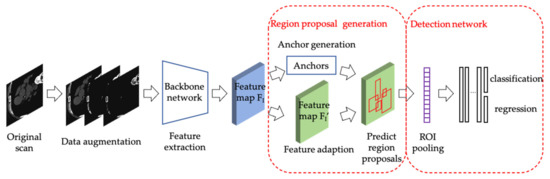
Figure 1. The framework of the proposed automatic method.

3.1. Data Augmentation

Deep learning training requires a lot of labeled data. It is difficult to obtain medical images. Labeled medical images are more difficult to obtain because they require professionals to the label. The data augmentation method used in natural images may affect the detection accuracy in medical images. To increase the number of images without affecting the accuracy of calcified plaque detection, we propose a data augmentation method with merging the prior knowledge of calcified plaque.

The train set we used is expressed as follow:

$$I_{\mathit{pri\_k}} = \left\{I_{\mathit{original}}, I_{\mathit{threshold}}, I_{\mathit{equalization}}\right\}$$

(1)

where $I_{original}$ is a collection of original labeled CT images. $I_{threshold}$ is $I_{original}$ after threshold processing. Calcium appears bright on a CT image, that is, it has a high CT Hounsfield unit. In [6], the threshold is set to 130 HU. A calcified plaque is defined as an area (≥1 mm²) in which all pixels are with a CT density above 130 HU. We use the calcified plaque definition as prior knowledge of the detection model. The prior knowledge is fused into the training process of the model by adding $I_{throuhold}$ in the train set. Every image in $I_{throuhold}$ is retaining the pixels with CT density greater than or equal to 130 HU and resetting pixels to 0 with CT density less than 130 HU, as follow:

$$\begin{array}{c}{\theta }_{threshold}=\left\{\begin{array}{c}0\hspace{1em}\hspace{1em}\hspace{1em}{\theta }_{original}<130 hu\hfill \\ {\theta }_{original}\hspace{1em}otherwise,\hfill \end{array}\right.\end{array}$$

(2)

where ${\theta }_{threshold}$ and ${\theta }_{original}$ is the CT value of the pixel in $I_{threshold}$ image and $I_{original}$ image respectively.

$I_{equalization}$ is the set of images after histogram equalization in $I_{threshold}$ Histogram equalization can increase image contrast and better detail in the images. The intensities can be better distributed on the histogram through histogram equalization. The conversion formula is as follow:

$$\begin{array}{c}{v}_{equalizaiton}^{k^{\prime }}=f\left(v_{threshold}^k\right)=\left(L-1\right)·{\displaystyle {\displaystyle \sum }_{i=0}^k}\frac{n_{threshold}^i}{N_{threshold}},\end{array}$$

(3)

where $k,k^{\prime }\in \left. [0,L-1\right]$, $L$ is the total number of gray levels in the image. $v^k$ is the gray value of image at $k$ level. $n^i$ is the number of occurrences at gray level $i$. $N$ is the total number of pixels in the image. $f$ is the histogram equalization function.

3.2. Detection Framework

Until now, there are two types of object detection CNN models, one-stage learning and two-stage learning. The Faster R-CNN [24] we adopted is a widespread object detection CNN framework and belongs to two-stage learning. The one-stage detector is generally faster but less accurate than the two-stage detector. Medical images require higher precision, not faster speed. Consequently, we adopt Faster R-CNN to detect calcified plaque in CT images.

Faster R-CNN model workflow includes the backbone for feature extraction, RPN for region proposal generation, and detection network for classification and regression. In feature extraction, Faster R-CNN uses a backbone network to extract feature maps of input images. The feature maps are shared for subsequent RPN and RoIHead. RPN generated nine anchors centered on every pixel of the feature map. For a convolutional feature map of size W × H, there are 9 × W × H anchors in total. $N_{cls}$ out of 9 × W × H anchors were selected to participate in RPN training. After RPN training, a set of region proposals is obtained. The detection network classifies the region proposals and regresses the bounding boxes of region proposals.

3.3. Region Proposal Generation

In a two-stage object detection framework, the anchors generated by region proposal generation are used as the input of the detection network for classification and regression. Therefore, the quality of anchors has a significant influence on the final detection result. RPN in Faster R-CNN generates a large set of densely distributed anchors with sliding windows. Only a few anchors are related to the regions of interest. A large of useless anchors caused computational cost. Therefore, Wang, J et al. [7] proposed guided anchoring, a more effective region proposal generation method.

The guided anchoring method generated sparse anchors that may contain objects instead of roughly generating even anchors. Firstly, the guided anchoring method used an image pyramid to build a feature pyramid. Secondly, for each output feature map of the feature pyramid, the anchor location and shape were predicted by two sub-networks branches. A feature adaption module applied deformable convolution to the original feature map to obtain an adapted feature map. Finally, classification and bounding-box regression were performed on the adapted feature map. There are three steps to generate anchors as follows.

Anchor location prediction. For each output feature map $F_I$ of the feature pyramid, anchor location prediction branch using a sub-network to obtain the probability map $p(i, j| F_I)$, where $\left(i,j\right)$ is the coordinate on $F_I$.

Anchor shape prediction. For each output feature map $F_I$ of the feature pyramid, anchor shape prediction branch using a sub-network to predict the best shape $\left(w, h\right)$ for each location, where $\left(w, h\right)$ is the width and height of anchor. The branch outputs $\left(dw, dh\right)$ and uses the transformation $w=\sigma ·s·e^{dw}, h=\sigma ·s·e^{dh}$ to obtain $\left(w, h\right)$, where $s$ is the stride and $\sigma$ is an empirical scale factor.

Anchor-guided feature adaption. Since each anchor has a different shape at the corresponding location, the original feature map cannot be used to obtain the region proposal. Anchor-guided feature adaption branch applies a $3\times 3$ deformable convolutional layer to transform the feature $f_i$ based at the $i$-th location $f_i{}^{\prime }=N_T\left(f_i, w_i,h_i\right)$, where $f_i{}^{\prime }$ is the transformed feature and $(w_i,h_i)$ is the corresponding anchor shape.

4. Experiments and Results

4.1. Dataset

CT is commonly used in clinical examination of the coronary arteries, which allows for noninvasive detection and characterization of calcified plaques. Coronary CT is a widely used imaging examination, and it is an essential basis for doctors to confirm the diagnosis. In clinical, calcified plaque is typically measured on ECG-gated 3 mm CT images [29].

OrCaScore [30] is a public dataset of calcified plaque scores. There is a non-contrast-enhanced calcium scoring CT (CSCT) and a corresponding contrast-enhanced cardiac computed tomography angiography (CCTA) of each patient. As described in [30], the train set includes 32 patients CSCT and CCTA, and the test set includes 40 patients’ images. Images in the dataset were acquired on four different CT scanners from four different vendors in four different hospitals. Patients were scanned on a multidetector-row CT scanner from one of the four different vendors (Lightspeed VCT, software version gmp vct. 26, GE Healthcare, Milwaukee, WI, USA; Brilliance iCT, software version 3.2.0, Philips Healthcare, Best, The Netherlands; SOMATOM Definition Flash, software version syngo ct 2010A, Siemens Healthcare, Forchheim, Germany; and Aquilion ONE, software version 4.93, Toshiba Medical Systems, Otawara, Japan).

In clinical practice, not every patient can undergo a CCTA scan. Many patients only receive CSCT with a lower radiation dose if the patient cannot receive the iodine-containing contrast material as an intravenous (IV) injection. Therefore, we used only the CSCT of the OrCaScore train set.

Unprocessed data is CT volume data in DICOM format. Digital Imaging and Communications in Medicine (DICOM) is the standard for the communication and management of medical imaging information and related data. Each patient corresponds to a DICOM file. A DICOM file consists of a number of attributes, including items such as name, ID, pixel information, etc. We extract axial slices from the CT volume data. We convert the slices to grayscale images with 8-bit. Images with no calcified plaques are eliminated. The dataset $I_{original}$ consists of 180 images that contain calcified plaques. After data augmentation in Section 2.1, there are 432 images in the train set and 36 images in the test set. The size of the image is 512 × 512. The number of images in each set of the original dataset $I_{original}$ and dataset with prior knowledge $I_{pri\_k}$.is shown in Table 1.

Table 1. The number of images in each set.

Dataset	Train Set	Test Set
$I_{original}$	144	36
$I_{pri\_k}$	432	36

orCaScore is a voxel-level segmentation dataset, and we transform it into a lesion-level detection dataset by adding a bounding box outside of every lesion in the reference standard. Figure 2 shows an example of an image and corresponding ground truth.

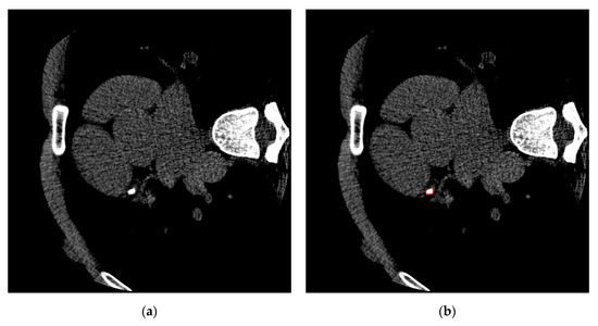
Figure 2. An example of an image and corresponding ground truth. (a) An image of one patient in orCaScore. (b) The corresponding ground truth, the red bounding box points out the calcified plaques in this image.

4.2. Performance Metrics

We use a confusion matrix to present a visualization of algorithm performance. Each column represents the predicted value, and each row represents the actual category. Such as Table 2.

Table 2. Performance confusion matrix.

	Detection	Positive	Negative
Ground Truth
positive		true positive	false negative
negative		false positive	true negative

The conditions for correct prediction are below:

• The category is correct, and the confidence is more significant than a certain threshold. In our experiments, the threshold is 0.5.
• The IoU of the prediction box and the ground truth box is more significant than a certain threshold, IoU_threshold which is set as 0.5 in the experiments. The intersection ratio IoU measures the degree of overlap between the two regions and is the overlap of the two regions occupying the total area.

$$\begin{array}{c}Io{U}_{A,B}= \frac{A\cap B}{A\cup B},\end{array}$$

(4)

where $Io{U}_{A, B}$ is the intersection ratio IoU between bounding box $A$ and ground truth $B$.

In the evaluation, there are three classifications of every bounding box predicted by our model. The bounding box which correctly identified calcified plaque is classified as Ture Positive (TP). The bounding box which identifies calcified plaque but is not in reference standard is classified as False Positive (FP). The bounding box which is calcified plaque but not identified is classified as False Negative (FN).

In the lesion objection, we want to reduce the probability of missed diagnosis as much as possible in clinical. We need to increase the true positives and decrease the false negatives. Therefore, we choose Average Precision (AP) and recall as the evaluation standard. AP measures the overall performance of the model, and recall measures the missed diagnosis of the model. The higher the AP and recall, the better the performance of the model.

Recall and AP are defined as the following formulas:

$$\begin{array}{c}Recall= \frac{True Positive}{Ture Positive+False Negative},\end{array}$$

(5)

$$\begin{array}{c}AP=\sum \left(R_n-R_{n-1}\right)P_{replace}\left(R_n\right),\end{array}$$

(6)

where $P$ and $R$ are Precision and Recall, respectively. $R_n$ is the Recall value at the n-th threshold. $P\left(R\right)$ is the Precision value at the corresponding recall. The precision and $P_{replace}\left(R\right)$ are defined as follows.

$$\begin{array}{c}Precision=\frac{True Positive}{Ture Positive+False Postive},\end{array}$$

(7)

$$\begin{array}{c}{P}_{replace}\left(R\right)=\underset{R^{\prime }\ge R}{\max }P\left(R^{\prime }\right).\end{array}$$

(8)

4.3. Experiment Implementation Details

4.3.1. Training Hyper-Parameters

All experiments are run on Ubuntu 18.04 with Python 3.7. Our experiments are implemented with PyTorch. We trained on 4 NVIDIA Geforce 2080ti GPUs with 2 images per GPU. We use the ResNet50 [31] with Feature Pyramid Network(FPN) [32] as the backbone architecture. The learning rate is initialized to 0.01 and decreased by 0.1 at epoch 8 and 11. The coding is implemented based on a public platform, MMDetection [33]. The Hyper-parameters detail is as Table 3.

Table 3. The hyper-parameters detail.

Stage	Hyper-Parameter	Value
SGD Optimizer	Learning rate	0.01
	Weight decay	0.0001
	Momentum	0.9
Training	Epochs	20
	Batch-size	8
Scale	$\sigma$	4

4.3.2. Loss Function

The loss function in the end-to-end training is a multi-task loss. There are two parts to the detection framework, region proposal generation, and detection network. In region proposal generation, since the center region of the object usually occupies a small part of a whole picture, the loss ${\mathcal{L}}_{loc}$ for anchor location prediction branch is Focal Loss [34]:

$$\begin{array}{c}{\mathcal{L}}_{loc}=\left\{\begin{array}{c}-\alpha {\left(1-p\right)}^{\gamma }\log \left(p\right)\hspace{1em}\hspace{1em}\hspace{1em}if y=1\hfill \\ -\left(1-\alpha \right)p^{\gamma }\log \left(1-p\right)\hspace{1em}otherwise,\hfill \end{array}\right.\end{array}$$

(9)

where $y\in \left\{\pm 1\right\}$ is the label representing whether the pixel belongs to the center region of the object and $p\in \left. [0,1\right]$ is the probability for the class with label $y=1$. $\alpha$ and $\gamma$ are weighting factors, and the values are 0.25 and 2.0 in the experiments, respectively.

The loss ${\mathcal{L}}_{shape}$ for anchor shape prediction branch is bounded iou loss which is defined as:

$$\begin{array}{c}{\mathcal{L}}_{shape}= {\mathcal{L}}_1\left(1-\min \left(\frac{w}{w_g}, \frac{w_g}{w}\right)\right)+{\mathcal{L}}_1\left(1-\min \left(\frac{h}{h_g}, \frac{h_g}{h}\right)\right),\end{array}$$

(10)

where ${\mathcal{L}}_1$ is the smooth L1 loss, $\left(w, h\right)$ and $\left(w_g, h_g\right)$ are the predicted anchor shape and the corresponding ground truth bounding box shape.

In the detection network, the loss ${\mathcal{L}}_{cls}$ and ${\mathcal{L}}_{reg}$ are cross-entropy loss and smooth L1 loss, respectively.

The final joint training loss is as follows:

$$\begin{array}{c}\mathcal{L}= {\lambda }_1{\mathcal{L}}_{loc}+{\lambda }_2{\mathcal{L}}_{shape}+{\mathcal{L}}_{cls}+{\mathcal{L}}_{reg}.\end{array}$$

(11)

where both ${\lambda }_1$ and ${\lambda }_2$ are 1 in the experiments.

4.4. Calcified Plaque Detection Result

We compare the six methods in the experiment, Faster R-CNN with RPN, K. Chellamuthu et al. [22] which is introduced in Section 2.2, DetectoRS [35], Libra R-CNN [36], CARAFE [37], and Faster R-CNN with guided anchoring employed in this paper. We train and test the six methods with two datasets, respectively, the original dataset $I_{original}$ and dataset with prior knowledge $I_{pri\_k}$.

Table 4 shows that the performance of Faster R-CNN with guided anchoring trained on the dataset $I_{pri\_k}$ is superior to that of the other methods. Of the methods considered, the method proposed in this study has the highest recall and AP. As pointed out in Table 4, guided anchoring increases recall to 0.814 and AP to 0.724 instead of RPN, although two sequential Faster R-CNN increase recall from 0.744 to 0.756 and AP from 0.554 to 0.567. Guided anchoring uses fewer parameters and faster speed to get better performance. Although the recall of Libra R-CNN and CARAFE is higher than Faster R-CNN with guided anchoring, we can see from the lower AP of Libra R-CNN and CARAFE that the high recall is obtained through the generation of a large number of predicted bounding boxes to prevent missed detection. Therefore, Faster R-CNN with guided anchoring performs better from the better AP, which measures the model’s overall performance.

Table 4. The comparison results of Faster R-CNN with RPN, K. Chellamuthu et al., DetectoRS, Libra R-CNN, CARAFE, and Faster R-CNN with guided anchoring trained on original dataset and dataset with prior knowledge, respectively. CI = confidence interval.

Method	Dataset	Recall (95% CI)	AP
Faster R-CNN with RPN	$I_{original}$	0.530 (0.404–0.653)	0.296
	$I_{pri\_k}$	0.744 (0.671–0.806)	0.554
K. Chellamuthu et al. [22]	$I_{original}$	0.561 (0.433–0.680)	0.362
	$I_{pri\_k}$	0.756 (0.683–0.755)	0.567
DetectoRS [35]	$I_{original}$	0.621 (0.493–0.735)	0.434
	$I_{pri\_k}$	0.737 (0.669–0.796)	0.594
Libra R-CNN [36]	$I_{original}$	0.652 (0.523–0.762)	0.409
	$I_{pri\_k}$	0.872 (0.811–0.916)	0.593
CARAFE [37]	$I_{original}$	0.697 (0.570–0.801)	0.524
	$I_{pri\_k}$	0.820 (0.752–0.873)	0.656
Faster R-CNN with guided anchoring	$I_{original}$	0.576 (0.448–0.694)	0.379
	$I_{pri\_k}$	0.814 (0.746–0.868)	0.724

The role of data augmentation with prior knowledge is also reflected in Table 4. From the experiment result, we can see that the results of the three methods trained on the dataset $I_{pri\_k}$ greatly surpassed that trained on the dataset $I_{original}$. Especially in Faster R-CNN with guided anchoring, the recall increases from 0.576 to 0.814, and AP increases from 0.379 to 0.724. The data augmentation with prior knowledge can significantly improve the calcified plaque detection performance.

Figure 3 and Figure 4 are the detection results comparing Faster R-CNN and Faster R-CNN with guided anchoring of the same image. The result images are cropped to see clearly. Figure 3 shows the situation of missed detection in the experiment of Faster R-CNN. The false-negative of Faster R-CNN (Figure 4a) is detected by Faster R-CNN with guided anchoring (Figure 4b). Figure 4 shows two examples of reducing redundant detection of Faster R-CNN with guided anchoring. Moreover, both in the two examples of Figure 4, the calcified plaques detected by Faster R-CNN with Guided Anchoring have a higher classification score than by Faster R-CNN.

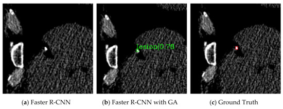
Figure 3. Missed detection of Faster R-CNN. (a) The detection result of Faster R-CNN. The calcified plaque is not detected. (b) The detection result of Faster R-CNN with guided anchoring. (c) The ground truth of the image. The ground truth is labeled by the red bounding box and pointed out by a red arrow.

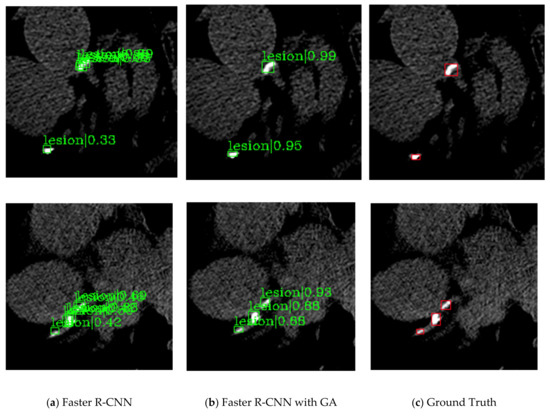
Figure 4. Two examples of the redundant detection of Faster R-CNN. (a) The detection results of Faster R-CNN. (b) The detection results of faster R-CNN with guided anchoring. (c) The ground truths of the images.

4.5. Analysis of Improvement

Table 5 lists the comparison result of different backbone in the detection framework. In the experiment of our proposed method, we choose four popular CNN architectures as backbone, ResNet50, ResNet101, ResNeXt101_32 × 4d and ResNeXt101_64 × 4d. As pointed as Table 5, ResNet101 as the backbone network has the best result in both recall and AP. Therefore, it is not that the more complex the network has better results. Over-fitting caused by an overly complex network makes recall and AP drop.

Table 5. Results of different backbones.

Backbone	Recall (95% CI)	AP
ResNet50	0.814 (0.746–0.868)	0.724
ResNet101	0.855 (0.791–0.902)	0.791
ResNeXt101_32 × 4d	0.779 (0.708–0.837)	0.652
ResNeXt101_64 × 4d	0.715 (0.640–0.780)	0.548

Table 6 shows the comparison result of a pre-trained network and a network trained from scratch. Here we use Faster R-CNN with guided anchoring trained on PASCAL VOC dataset as the pre-trained network. Table 6 results show that the pre-trained network has improved recall and AP compared to the network trained from scratch.

Table 6. Comparison of a pre-trained network and a network trained from scratch.

Method	Recall (95% CI)	AP
trained from scratch	0.814 (0.746–0.868)	0.724
pre-trained	0.843 (0.778–0.892)	0.777

Table 7 shows the impact of the hyper-parameter scale value at 2, 4, 6, 8. The scale is a hyper-parameter representing the size range of the anchor, detail in Section 3.3. Since the size of the calcified plaques is smaller than most objects in natural images, the model has the best performance when the scale value is 2 as pointed out in Table 7.

Table 7. The impact of the scale on the model performance.

Scale	Recall (95% CI)	AP
2	0.855 (0.791–0.902)	0.798
4	0.814 (0.746–0.868)	0.724
6	0.756 (0.683–0.817)	0.692
8	0.686 (0.610–0.753)	0.575

5. Conclusions

We have presented a method with prior knowledge to automatically detect calcified plaque of coronary arteries in non-contrast-enhanced cardiac CT. Our proposed method expands the training data by adding prior knowledge and improves the performance of the calcified plaque detection task. The method employs guided anchoring as the region proposal generation network in Faster R-CNN. In the comparing of the RPN, guided anchoring can solve the problem of anchor box redundancy. Compared with other methods, our method gets better results.

References

- Naghavi, M.; Wang, H.; Lozano, R.; Davis, A.; Liang, X.; Zhou, M.; Vollset, S.E.; Abbasoglu Ozgoren, A.; Abdalla, S.; Abd-Allah, F.; et al. Global, regional, and national age-sex specific all-cause and cause-specific mortality for 240 causes of death, 1990–2013: A systematic analysis for the Global Burden of Disease Study 2013. Lancet 2015, 385, 117–171. [Google Scholar]
- Detrano, R.; Guerci, A.D.; Carr, J.J.; Bild, D.E.; Burke, G.; Folsom, A.R.; Liu, K.; Shea, S.; Szklo, M.; Bluemke, D.A.; et al. Coronary calcium as a predictor of coronary events in four racial or ethnic groups. N. Engl. J. Med. 2008, 358, 1336–1345. [Google Scholar] [CrossRef]
- Liu, W.; Zhang, Y.; Yu, C.M.; Ji, Q.W.; Cai, M.; Zhao, Y.X.; Zhou, Y.J. Current understanding of coronary artery calcification. J. Geriatr. Cardiol. 2015, 12, 668–675. [Google Scholar] [PubMed]
- Hu, S.; Gao, Y.; Niu, Z.; Jiang, Y.; Li, L.; Xiao, X.; Wang, M.; Fang, E.F.; Menpes-Smith, W.; Xia, J.; et al. Weakly Supervised Deep Learning for COVID-19 Infection Detection and Classification from CT Images. IEEE Access 2020, 8, 118869–118883. [Google Scholar] [CrossRef]
- Saeedizadeh, N.; Minaee, S.; Kafieh, R.; Yazdani, S.; Sonka, M. COVID TV-UNet: Segmenting COVID-19 chest CT images using connectivity imposed U-Net. arXiv 2020, arXiv:2007.12303. [Google Scholar]
- Agatston, A.S.; Janowitz, W.R.; Hildner, F.J.; Zusmer, N.R.; Viamonte, M.; Detrano, R. Quantification of coronary artery calcium using ultrafast computed tomography. J. Am. Coll. Cardiol. 1990, 15, 827–832. [Google Scholar] [CrossRef]
- Wang, J.; Chen, K.; Yang, S.; Loy, C.C.; Lin, D. Region proposal by guided anchoring. Proc. IEEE Comput. Soc. Conf. Comput. Vis. Pattern Recognit. 2019, 2019, 2960–2969. [Google Scholar]
- Išgum, I.; Rutten, A.; Prokop, M.; Staring, M.; Klein, S.; Pluim, J.P.; Viergever, M.A.; van Ginneken, B. Automated aortic calcium scoring on low-dose chest computed tomography. Med. Phys. 2010, 37, 714–723. [Google Scholar] [CrossRef]
- Išgum, I.; van Ginneken, B.; Viergever, M.A. Automatic detection of calcifications in the aorta from abdominal CT scans. Int. Congr. Ser. 2003, 1256, 1037–1042. [Google Scholar] [CrossRef]
- Išgum, I.; Prokop, M.; Niemeijer, M.; Viergever, M.A.; Van Ginneken, B. Automatic coronary calcium scoring in low-dose chest computed tomography. IEEE Trans. Med. Imaging 2012, 31, 2322–2334. [Google Scholar] [CrossRef]
- Wolterink, J.M.; Leiner, T.; Takx, R.A.P.; Viergever, M.A.; Išgum, I. Automatic Coronary Calcium Scoring in Non-Contrast-Enhanced ECG-Triggered Cardiac CT with Ambiguity Detection. IEEE Trans. Med. Imaging 2015, 34, 1867–1878. [Google Scholar] [CrossRef] [PubMed]
- Yang, G.; Chen, Y.; Ning, X.; Sun, Q.; Shu, H.; Coatrieux, J.L. Automatic coronary calcium scoring using noncontrast and contrast CT images. Med. Phys. 2016, 43, 2174–2186. [Google Scholar] [CrossRef] [PubMed]
- Durlak, F.; Wels, M.; Schwemmer, C.; Sühling, M.; Steidl, S.; Maier, A. Growing a random forest with Fuzzy spatial features for fully automatic artery-specific coronary calcium scoring. Lect. Notes Comput. Sci. (Incl. Subser. Lect. Notes Artif. Intell. Lect. Notes Bioinform.) 2017, 10541, 27–35. [Google Scholar]
- Acharya, U.R.; Meiburger, K.M.; Koh, J.E.W.; Ciaccio, E.J.; Vicnesh, J.; Tan, S.K.; Wong, J.H.D.; Aman, R.R.A.R.; Ng, K.H. Automated detection of calcified plaque using higher-order spectra cumulant technique in computer tomography angiography images. Int. J. Imaging Syst. Technol. 2019, 30, 285–297. [Google Scholar] [CrossRef]
- Mirsky, Y.; Mahler, T.; Shelef, I.; Elovici, Y. CT-GAN: Malicious tampering of 3D medical imagery using deep learning. In Proceedings of the 28 USENIX Security Symposium, Santa Clara, CA, USA, 14–16 August 2019; pp. 461–478. [Google Scholar]
- Prasoon, A.; Petersen, K.; Igel, C.; Lauze, F.; Dam, E.; Nielsen, M. Deep feature learning for knee cartilage segmentation using a triplanar convolutional neural network. Lect. Notes Comput. Sci. (Incl. Subser. Lect. Notes Artif. Intell. Lect. Notes Bioinform.) 2013, 8150, 246–253. [Google Scholar]
- Lessmann, N.; Išgum, I.; Setio, A.A.A.; de Vos, B.D.; Ciompi, F.; de Jong, P.A.; Oudkerk, M.; Mali, W.P.T.M.; Viergever, M.A.; van Ginneken, B. Deep convolutional neural networks for automatic coronary calcium scoring in a screening study with low-dose chest CT. In Medical Imaging 2016: Computer-Aided Diagnosis; International Society for Optics and Photonics: San Diego, CA, USA, 2016; Volume 9785, p. 978511. [Google Scholar]
- Wolterink, J.M.; Leiner, T.; de Vos, B.D.; van Hamersvelt, R.W.; Viergever, M.A.; Išgum, I. Automatic coronary artery calcium scoring in cardiac CT angiography using paired convolutional neural networks. Med. Image Anal. 2016, 34, 123–136. [Google Scholar] [CrossRef]
- Lessmann, N.; Van Ginneken, B.; Zreik, M.; De Jong, P.A.; De Vos, B.D.; Viergever, M.A.; Išgum, I. Automatic Calcium Scoring in Low-Dose Chest CT Using Deep Neural Networks with Dilated Convolutions. IEEE Trans. Med. Imaging 2018, 37, 615–625. [Google Scholar] [CrossRef]
- Gernaat, S.A.M.; van Velzen, S.G.M.; Koh, V.; Emaus, M.J.; Išgum, I.; Lessmann, N.; Moes, S.; Jacobson, A.; Tan, P.W.; Grobbee, D.E.; et al. Automatic quantification of calcifications in the coronary arteries and thoracic aorta on radiotherapy planning CT scans of Western and Asian breast cancer patients. Radiother. Oncol. 2018, 127, 487–492. [Google Scholar] [CrossRef]
- Liu, J.; Lu, L.; Yao, J.; Bagheri, M.; Summers, R.M. Pelvic artery calcification detection on CT scans using convolutional neural networks. In Medical Imaging 2017: Computer-Aided Diagnosis; International Society for Optics and Photonics: San Diego, CA, USA, 2017; Volume 10134, p. 101341A. [Google Scholar]
- Chellamuthu, K.; Liu, J.; Yao, J.; Bagheri, M.; Lu, L.; Sandfort, V.; Summers, R.M. Atherosclerotic vascular calcification detection and segmentation on low dose computed tomography scans using convolutional neural networks. In Proceedings of the 2017 IEEE 14th International Symposium on Biomedical Imaging (ISBI 2017), Melbourne, Australia, 18–21 April 2017; pp. 388–391. [Google Scholar]
- Girshick, R.; Donahue, J.; Darrell, T.; Malik, J. Rich feature hierarchies for accurate object detection and semantic segmentation. In Proceedings of the IEEE conference on computer vision and pattern recognition 2014, Columbus, OH, USA, 23–28 June 2014; pp. 580–587. [Google Scholar]
- Ren, S.; He, K.; Girshick, R.; Sun, J. Faster R-CNN: Towards real-time object detection with region proposal networks. Adv. Neural Inf. Process. Syst. 2015, 2015, 91–99. [Google Scholar] [CrossRef]
- Zreik, M.; Van Hamersvelt, R.W.; Wolterink, J.M.; Leiner, T.; Viergever, M.A.; Išgum, I. A Recurrent CNN for Automatic Detection and Classification of Coronary Artery Plaque and Stenosis in Coronary CT Angiography. IEEE Trans. Med. Imaging 2019, 38, 1588–1598. [Google Scholar] [CrossRef]
- Fischer, A.M.; Eid, M.; De Cecco, C.N.; Gulsun, M.A.; Van Assen, M.; Nance, J.W.; Sahbaee, P.; De Santis, D.; Bauer, M.J.; Jacobs, B.E.; et al. Accuracy of an Artificial Intelligence Deep Learning Algorithm Implementing a Recurrent Neural Network with Long Short-term Memory for the Automated Detection of Calcified Plaques from Coronary Computed Tomography Angiography. J. Thorac. Imaging 2020, 35, S49–S57. [Google Scholar] [CrossRef] [PubMed]
- Liu, J.; Wang, D.; Lu, L.; Wei, Z.; Kim, L.; Turkbey, E.B.; Sahiner, B.; Petrick, N.A.; Summers, R.M. Detection and diagnosis of colitis on computed tomography using deep convolutional neural networks. Med. Phys. 2017, 44, 4630–4642. [Google Scholar] [CrossRef] [PubMed]
- Yazdani, S.; Minaee, S.; Kafieh, R.; Saeedizadeh, N.; Sonka, M. COVID CT-Net: Predicting Covid-19 from Chest CT Images Using Attentional Convolutional Network. arXiv 2020, arXiv:2009.05096. [Google Scholar]
- Hughes-Austin, J.M.; Dominguez, A.; Allison, M.A.; Wassel, C.L.; Rifkin, D.E.; Morgan, C.G.; Daniels, M.R.; Ikram, U.; Knox, J.B.; Wright, C.M.; et al. Relationship of Coronary Calcium on Standard Chest CT Scans With Mortality. JACC Cardiovasc. Imaging 2016, 9, 152–159. [Google Scholar] [CrossRef]
- Wolterink, J.M.; Leiner, T.; De Vos, B.D.; Coatrieux, J.L.; Kelm, B.M.; Kondo, S.; Salgado, R.A.; Shahzad, R.; Shu, H.; Snoeren, M.; et al. An evaluation of automatic coronary artery calcium scoring methods with cardiac CT using the orCaScore framework. Med. Phys. 2016, 43, 2361–2373. [Google Scholar] [CrossRef] [PubMed]
- He, K.; Zhang, X.; Ren, S.; Sun, J. Deep residual learning for image recognition. Proc. IEEE Comput. Soc. Conf. Comput. Vis. Pattern Recognit. 2016, 2016, 770–778. [Google Scholar]
- Lin, T.Y.; Dollár, P.; Girshick, R.; He, K.; Hariharan, B.; Belongie, S. Feature pyramid networks for object detection. In Proceedings of the IEEE Conference on Computer Vision and Pattern Recognition 2017, Honolulu, HI, USA, 21–26 July 2017; pp. 936–944. [Google Scholar]
- Chen, K.; Wang, J.; Pang, J.; Cao, Y.; Xiong, Y.; Li, X.; Sun, S.; Feng, W.; Liu, Z.; Xu, J.; et al. MMDetection: Open MMLab Detection Toolbox and Benchmark. arXiv 2019, arXiv:1906.07155. [Google Scholar]
- Lin, T.Y.; Goyal, P.; Girshick, R.; He, K.; Dollar, P. Focal Loss for Dense Object Detection. IEEE Trans. Pattern Anal. Mach. Intell. 2020, 42, 318–327. [Google Scholar] [CrossRef]
- Qiao, S.; Chen, L.C.; Yuille, A. DetectoRS: Detecting objects with recursive feature pyramid and Switchable Atrous Convolution. arXiv 2020, arXiv:2006.02334. [Google Scholar]
- Pang, J.; Chen, K.; Shi, J.; Feng, H.; Ouyang, W.; Lin, D. Libra R-CNN: Towards balanced learning for object detection. Proc. IEEE Comput. Soc. Conf. Comput. Vis. Pattern Recognit. 2019, 2019, 821–830. [Google Scholar]
- Wang, J.; Chen, K.; Xu, R.; Liu, Z.; Loy, C.C.; Lin, D. CARAFE: Content-aware reassembly of features. Proc. IEEE Int. Conf. Comput. Vis. 2019, 2019, 3007–3016. [Google Scholar]
Publisher’s Note: MDPI stays neutral with regard to jurisdictional claims in published maps and institutional affiliations. |
© 2020 by the authors. Licensee MDPI, Basel, Switzerland. This article is an open access article distributed under the terms and conditions of the Creative Commons Attribution (CC BY) license (http://creativecommons.org/licenses/by/4.0/).