Multi-Hop Dynamic Map Data Propagation Algorithm for Clustered Vehicular Networks

Abstract

To ensure the driving safety in vehicular network, it is necessary to construct a local dynamic map (LDM) for an extended range. Using the standard vehicular communication protocols, however, vehicles can construct the LDM for only one-hop range. Constructing large-scale LDM is highly challenging because vehicles randomly change their position. This paper proposes a dynamic map propagation (DMP) method, which builds a large aggregated LDM data using a multi-hop communication. To reduce the data overhead, we introduce an efficient clustering method based on a half-circle of the forwarder’s wireless range. The DMP elects one forwarder per cluster, which constructs LDM and forwards it to a neighbor cluster. The inter-cluster interference is minimized by allocating a different transmit window to each cluster. DMP copes with a dynamic environment by frequently re-electing the forwarders and their associated transmission windows. Simulation results reveal that DMP enhances the forwarders’ reception ratio by 20%, while extending LDM dissemination range by 29% over a previous work.

1. Introduction

A self-organized dynamic vehicular network supports various types of communications [1,2]. The communication links between the vehicles can significantly improve the driving safety and traffic control [3]. A vehicle-to-everything (V2X) network supports various types of safety applications which can be utilized to warn the drivers about potential dangers. All safety applications, however, rely on recent dynamic information exchanged between the vehicles via vehicle-to-vehicle (V2V) or vehicle-to-infrastructure (V2I) networks. This dynamic information can be represented as a map which is updated every predefined period to cope with dynamic nature of V2X network. This map is called as a local dynamic map (LDM) and its standard definition is given in [4]. The LDM contains static and dynamic components of the roads. Using the LDM, each vehicle can discover its surrounding neighbors and identify the recent changes on the road. The LDM can be constructed at various scale using V2X technologies. V2X can also be considered as a key technology that enhances a driving safety.

Every year, road accidents cause approximately 1.35 million deaths worldwide (on the average 3700 people lose their lives every day on the roads) [5]. In order to reduce the sudden maneuvers (lane change, abrupt speed change, emergency brake) that cause the accidents, each vehicle needs to share its mobility updates with other vehicles. According to IEEE 1609 and ETSI 102 687 standards [1,2], each vehicle periodically broadcasts a basic safety message (BSM) to announce the latest dynamic updates within one-hop communication range [6]. Using the BSM messages, each vehicle can build its own one-hop range LDM dataset and exploit it while avoiding potential threats. However, one-hop range LDM data may not be sufficient to ensure road safety. In order to create a multi-hop range LDM dataset, vehicles can disseminate their one-hop range LDM data via a multi-hop process.

Both V2V and V2I can be used for data dissemination in the vehicular network [7,8]. In this paper, we consider only V2V communication for simplicity, while it can be easily extended to networks with both V2V and V2I. During the multi-hop LDM data dissemination, however, a standard V2V communication protocol may not guarantee an expected performance since it suffers from a hidden node collision—two vehicles transmitting packets at the same time cause collision at the common receivers.

To ensure the driving safety and enhance the traffic management, the proposed method propagates one-hop range LDM data to construct the multi-hop LDM data. In our method, we use a clustering method to propagate map information in a multi-hop fashion, so each vehicle can obtain the latest position and mobility information of all remote vehicles (vehicles located beyond the communication range). It introduces novel algorithms to avoid the hidden terminal collision and mitigates the interference between the clusters (hereafter, we call it inter-cluster interference). The main contributions of the proposed method are as follows:

• It introduces a new efficient clustering method which significantly reduces data overhead in multi-hop LDM transmission.
• It employs a low-cost forwarder election algorithm that elects the optimum set of forwarders.
• To reduce an inter-cluster interference, it presents a cluster coloring algorithm that allocates optimal transmit windows to adjacent clusters.
• It maximizes the inter-cluster transmit window (color) reuse factor by re-allocating their colors.
• The proposed algorithm improves the range of multi-hop propagation and reduces the interference among hidden terminals.

The rest of the paper is organized as follows. Section 2 provides a review for the related works. Section 3 presents the network model for LDM construction, while Section 4 introduces the proposed clustering method. In Section 5, we describe a forwarder election algorithm; while in Section 6, we explain a transmit window allocation algorithm based on cluster coloring. Simulation results are shown in Section 7 followed by the conclusion and future work in Section 8.

2. Related Work

In vehicular network based on the ETSI 102 687 standard, each vehicle attempts to collect up-to-date information from surrounding vehicles. Then, the vehicle stores this information in LDM, which is employed while making driving decisions and avoiding accidents. The LDM is updated in every predefined period. Data stored in the LDM is divided into four levels: (1) permanent static, (2) transient static, (3) transient dynamic, and (4) highly dynamic [9], as presented in Figure 1. The first and second lowest levels represent the static map details such as roads, intersections, lanes, etc. The third and fourth levels contain the dynamic components of the map, such as a phase of a traffic signal, weather condition, and vehicles (position, speed, heading, etc.) on the road [9].

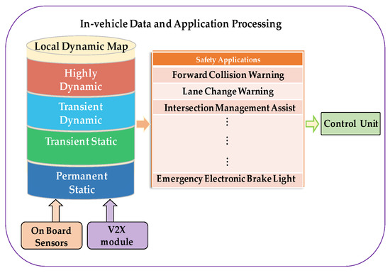
Figure 1. In-vehicle LDM data processing.

Many previous methods are primarily focused on the algorithms to improve the propagation of emergency packets with a few hundred bytes. In [10], the authors proposed a data propagation scheme that relies on V2V communications. In this work, the authors introduce so-called lateral crossing line (LCL) algorithm, which elects a set of relay vehicles to retransmit an emergency message in each hop. Based on the receivers’ location from the source of the emergency message, LCL calculates an overlapped area of the source’s and receiver’s wireless ranges and converts this area value into a back-off timer. If the receiver obtains the shortest back-off timer, then it becomes a relay vehicle for the corresponding hop. However, the authors of [10] did not consider an aggregation of one-hop safety messages and construction of LDM data. Moreover, their method did not specify the inter- and intra-cluster communications. They considered only propagation of small emergency messages generated by the particular vehicles in specific segments of the road.

Another promising study was conducted by Rayeni et al. [11]. Depending on the density, the authors proposed a dynamic partitioning scheme, which divides the backside of the transmitter’s wireless range into small partitions. These partitions associate with various forwarding priorities, which can be determined by assigning different back off timers. As the neighbor distance becomes further, it obtains a shorter back off timer. The length of each partition varies depending on the vehicle density. This scheme, however, assumes that there is always one spare radio which is utilized to generate a busy tone signal. This signal is expected to cover twice distance of the wireless range so that a hidden terminal problem can be resolved. Practically, this assumption can be considered as a waste of resources, and yet it may not provide a complete solution for a hidden node problem.

An infrastructure-based data propagation can enhance the coverage in a vehicular network. Therefore, the literature [12,13,14,15] contains many studies that introduce various approaches to use roadside units (RSUs) in message propagation. The authors of [12] introduced a delay-bound RSU-based data dissemination algorithm. For a given delay bound, this algorithm identifies an optimum number of RSUs to propagate the data in the pre-defined region. Similarly, authors in [13] developed heuristic algorithms to maximize the number of vehicles served by each RSUs in vehicular network. Some of the studies [14,15] formulated RSUs′ deployment problem as an integer linear problem (ILP). They proposed the particular configuration to enhance data propagation in a vehicular network. The authors of [12,13,14,15], however, made a tradeoff between the cost and data dissemination in the target region.

The authors of [7] proposed a method that combines V2I- and V2V-based data propagation. They deploy RSUs far enough from one another so that data between them can be exchanged through the V2V-based multi-hop communication. If there is neither a single-hop nor multi-hop communication link between the vehicles and RSU, the message can still be delivered to other RSUs through a carry-store-forward scheme [16]. An efficient data dissemination can also be organized through the clustering methods. The nodes can be grouped together into clusters, each of which contains one cluster head (CH) and group of member nodes. Normally, the CHs control data transmission and reception procedures. Authors in [17] proposed a hybrid architecture which combines Cellular V2X (C-V2X) and IEEE 802.11p with goal of achieving high packet reception ratio and low dissemination latency in multihop communication among the clusters. They minimized the usage of cellular infrastructure while propagating data in a multi-hop fashion. Their cluster selection technique utilizes the mobility information of the vehicles and selects the one which has a minimum average relative speed with other vehicles. The inter-cluster communication is conducted whether through predefined intermediate nodes or directly (direct connection of cluster head with another cluster) using LTE base stations.

In [18], authors introduced fuzzy inference system (FIS) to construct a clustered network to extend the network lifetime and reduce the packet loss. Their method applies a fuzzy logic to analyze various network parameters while choosing the CHs. Authors considered residual energy, moving speed, and pausing time of the nodes as the input parameters (descriptors) into FIS. Based on these descriptors, FIS outputs the probability (chance value) of nodes to be selected as CH. However, the clustering methods introduced in [18] are designed for fixed and less dynamic WSNs and hence, it may not produce an expected results for the high dynamic networks. Moreover, it did not consider inter-cluster message exchange which is an important process for our target application.

An interesting clustering approach was introduced in [19] where a distributed vehicular network was transformed into clustered network. The CHs are selected through the fitness value computed by each vehicle. In the initial stage, each vehicle discovers its neighbors by exchanging hello messages and then, each vehicle collects the following data: (1) time of transmission hello messages; (2) relative velocity; (3) an approximate link validity period; and (4) connectivity degree (density). Using this data, each vehicle calculates its fitness value and then broadcasts it to the neighbors. Then, the node with the smallest fitness value is selected as CH for the group of vehicles. In this method, the member vehicles may communicate with CHs directly or through relay nodes. It means the size of the cluster can be larger than the wireless range of the CH. However, the authors did not provide sufficient details about the intra-cluster communication process. In LDM construction, intra-cluster communication is a very crucial process.

Authors in [20] proposed a clustering-based multichannel medium access control (MAC) protocol to broadcast the safety messages. The authors differentiated the data traffic into two classes: (1) real-time traffic and (2) non-real time traffic. The CHs are defined by the timer-based election procedure. A new vehicle joins to the existing cluster if it receives an advertisement message within this timer. It becomes an independent cluster otherwise. Their MAC protocol maintains four different channels: (1) inter-cluster control channel; (2) inter-cluster data channel; (3) cluster-range control channel; and (4) cluster-range data channel. Inter-cluster control and cluster-range control channels are used for transmission of real-time traffics while the remaining channels are used for non-real time traffic. The vehicles access the cluster-range control channel through contention-free accessing mechanism while access to the inter-cluster control channel is conducted via a contention-based scheme. The authors applied code division multiplexing access (CDMA) mechanism to organize interference-free intra-cluster data (non-real time traffic) communication. As we can see, their MAC protocol combines various access mechanisms which makes the process of practical implementation very complex. In addition, to reduce hidden terminal interference, this protocol employs twice as much transmission power to conduct inter-cluster communication. However, the hidden terminal interference still may occur in larger scale (while sending aggregated LDM message) due to contention-based access mechanism. In this method, CH should manage resource allocation process in four different channels at a time which may become very complex in reality.

In [21], the authors presented a cluster-based beaconing algorithm that is aimed to provide local proximity maps to all vehicles. This local proximity map allows vehicles to detect the accidents in highway road. This algorithm aims to enhance the two criteria. First, the map used by the vehicles should have accurate details. Second, all vehicles in the vicinity should be coordinated with this map. It uses the cluster-based beaconing (aggregate-forward) scheme to distribute the vehicle proximity map. This scheme enhances the network performance since it uses different transmit windows during the data aggregation. After that, it selects a temporary forwarder that disseminates the map data in the common transmit window. Therefore, inter-cluster communication in this method degrades due to hidden terminal interference.

In most multi-hop data dissemination methods, vehicle information is disseminated through multiple transmissions conducted by selected forwarders. Since the transmissions are broadcast, the forwarders cannot verify whether their messages are successfully received by all target receivers. Moreover, in vehicular network, position of the vehicles frequently changes as they move with various velocity. Since vehicles’ data is propagated over the wireless channel, many factors can cause communication failure. One primary factor is the hidden terminal problem that creates severe interference and incurs significant packet reception loss. The hidden terminal problem often reduces the broadcast coverage by half [22,23].

Therefore, it is crucial to facilitate a robust and scalable propagation method to disseminate large-scale map data in multi-hop vehicular networks. Thus, we propose a dynamic map propagation (DMP) method which can cope with a hidden terminal effect and provides efficient LDM data propagation over the V2V links. It elects forwarders and constructs optimal clusters in a distributed vehicular network. We apply a cluster coloring technique that allocates colors to clusters as transmit window. Our proposed algorithm supports both the IEEE 1609 and ETSI 102 687 as underlying standard protocols.

3. Network Model

As a network model, we consider a multi-lane highway road shown in Figure 2. In our highway network model, we consider one direction at a time to construct individual clustered networks. Figure 2 considers only right direction lanes. The opposite direction can produce another clustered network in a similar fashion. To eliminate the interference, the vehicles travelling in the opposite direction may transmit their data over different channel. The road of Figure 2 contains a set of vehicles defined as $V=\left\{{\mathrm{v}}_1,{\mathrm{v}}_2,\dots ,{\mathrm{v}}_m\right\}$, where ${\mathrm{v}}_i$ represents an individual vehicle. Then, $V$ is divided into a set of clusters, which is represented by $S_{Total}=\left\{S_1,S_2,\dots ,S_m\right\}$ In Figure 2, our proposed clusters are denoted by solid half circles, whereas the full circle denotes the wireless range from each forwarder. A cluster $S_i$ comprises two types of nodes: (1) member nodes ${\mathrm{v}}_i$’s denoted by yellow triangles; and (2) forwarder node F_i denoted by red triangles. The forwarder node is elected among the member nodes that is located in the rear end of the cluster, as presented in Figure 2. The cluster size is denoted by the front half-circle of forwarder’s wireless range as indicated with the solid lines in Figure 2. We assume that all member nodes in the cluster travel in the same direction (towards the right direction as indicated by the triangles of the nodes). The clusters are separated by a set of inter-cluster gaps, $G_{Total}=\left\{g_1,g_2,\dots ,g_{m-1}\right\}$ where each $g_i$ represents the gap (or distances) between the forwarder $F_i$ of $S_i$ and the forwarder $F_{i+1}$ of $S_{i+1}$.

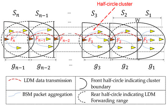
Figure 2. A clustered sub-network in multilane highway road.

Each vehicle is equipped with a V2X communication device. This device includes a global positioning system (GPS) receiver which provides an accurate time synchronization information. Hasan et al. [24] showed through real experiments that the GPS synchronization provides an accuracy of tens of nanoseconds which is sufficient to organize a slotted channel concept. The V2X device also broadcasts a basic safety message (BSM) over a predefined control channel using the IEEE 1609 standard [1]. The BSM message contains mobility details (position, velocity, acceleration, heading, steering wheel angle, yaw rate, etc.) of the transmitter node. The BSM is sent with a period $T_b$ (hereafter, it is referred as a beaconing period). Since each vehicle declares its mobility information inside the BSM message, the forwarders can easily identify the group of neighbors travelling in the same and opposite directions. From the received BSMs, each vehicle can also identify its leading and lagging (in behind) neighbors. Each forwarder $F_i$ collects BSM packets from all member nodes in its cluster $S_i$ indicated by solid half circles in Figure 2. From the collected BSM packets, $F_i$ of $S_i$ constructs the LDM data. Then, $F_i$ forwards this LDM data to the next (i.e., lagging) cluster $S_{i+1}$ which are indicated by the dotted half circles in Figure 2. This forwarding process is repeated through forwarders in multi-hops, so all vehicles in the lagging clusters can receive LDM data from the preceding neighbors. If a member vehicle ${\mathrm{v}}_i$ of the cluster $S_i$ changes its heading, then ${\mathrm{v}}_i$’s updated heading is included in its BSMs. Receiving the BSMs from ${\mathrm{v}}_i$, forwarder $F_i$ adds ${\mathrm{v}}_i$’s new heading information in the LDM and then forwards it to lagging clusters. If ${\mathrm{v}}_i$ drastically changes its heading (${\mathrm{v}}_i$ turns to different direction or road), then within the acceptable latency, this information is propagated to remote lagging vehicles inside the aggregated LDM packet. While transmitting the BSM packet, each member node conducts a contention-based broadcast within allocated transmit window. In this paper, we assume a fixed wireless range denoted as $W$ for simplicity of presentation. For other notations used in this study, reader can refer to Table 1.

Table 1. Brief description of notations

Symbols	Definition
$V$	Total number of vehicles
$S_{Total}=\left\{S_1,\dots ,S_m\right\}$	Set of clusters
$G_{total}=\left\{g_1,\dots ,g_{m-1}\right\}$	Set of inter-cluster gaps
${\mathrm{v}}_i$	Member vehicle of cluster $S_i$
$F_i$	Forwarder of cluster $S_i$
$F_{Lead}$	Leading forwarder
$F_{Lag}$	Lagging forwarder
$T_b$	Beaconing interval
$W$	Wireless range
$u_i$	Number of member vehicles in $S_i$
$u_{max}$	Maximum allowable number of vehicle in $S_i$
$h$	Number of hops
$N_C$	Number of colors
$T_i$	Transmit window $i$, $i\in N_C$
$C_i$	Color $i$, $i\in N_C$
$t_s$	Time slot
$M_{FDM}$	Forwarder designation message
$t_{DB}$	Distance-based forwarding timer
$T_{diss}$	Dissemination sub-window
$T_{agg}$	Aggregation sub-window

LDM Data Construction

In this paper, we consider two levels of LDM data construction. The first level is the construction of a one-hop range LDM data. This LDM data represents the dynamics details of single cluster. The second level is multi-hop range LDM data which comprises a set of one-hop range LDM data aggregated through multiple clusters. A multi-hop range LDM data can be constructed via a multi-hop propagation of one-hop range LDM packets.

As we mentioned, in a vehicular network, every vehicle broadcasts BSM [6] in every $T_b$ period. Taking advantage of this feature, a forwarder of each cluster can act as an aggregator of BSM packets received from its members. We use $u_i$ to denote the total number of member nodes within the cluster $S_i$. Then, in the first level, forwarder $F_i$ collects BSM data of $u_i$ members. Then, $F_i$ constructs a local LDM data of cluster $S_i$. Before forwarding the data, $F_i$ combines its LDM data with the one received from leading clusters. The LDM packet size is proportional to the number of vehicles $u_i$ in each cluster. The number of vehicles in the cluster is constrained by predefined $u_{max}$, which is mathematically defined by Equation (12) in Section 6. The aggregated LDM packet size is bounded by the acceptable range of the IEEE 1609 standard.

As the network density grows, the conventional protocols tend to suffer from serious performance loss due to hidden node problems. To reduce the hidden terminal interference, we partition $T_b$ into multiple transmit windows where each transmit window is assigned to specific cluster to perform the communication. One window can be assigned to multiple clusters as long as these clusters are far enough, so they do not interfere. For instance, in Figure 2, clusters $S_1$, $S_2$, and $S_3$ can be allocated to different transmit windows. Then, these clusters conduct their communication in the different transmit windows, and therefore, interference between these clusters can be significantly reduced.

4. Proposed Clustering Method

In this section, we first describe our novel clustering method. We then prove that our clustering method can reduce communication overhead (the time to transmit the redundant data) compared with a conventional clustering method.

As shown in Figure 3, our clustering method differs from the conventional clustering method utilized in [21,25]. In the conventional clustering method of Figure 3a, a cluster head (CH) considers all nodes within the wireless range as the cluster member nodes. Therefore, we refer to it as ‘full-circle clustering method’, since the wireless range of CH is assumed to be in circular shape. The CH communicates with neighbor CHs through a pair of gateways (GW). The CH organizes an intra-cluster communication session to collect the periodic packets of all member nodes. Then, it generates the LDM packet and then broadcasts it to all its member nodes. Upon receiving this packet, each GW node executes additional broadcast to forward the received LDM packet to neighboring clusters. In the full-circle clustering method, the LDM packet of each cluster must be transmitted three times in order to deliver this LDM data to neighboring clusters.

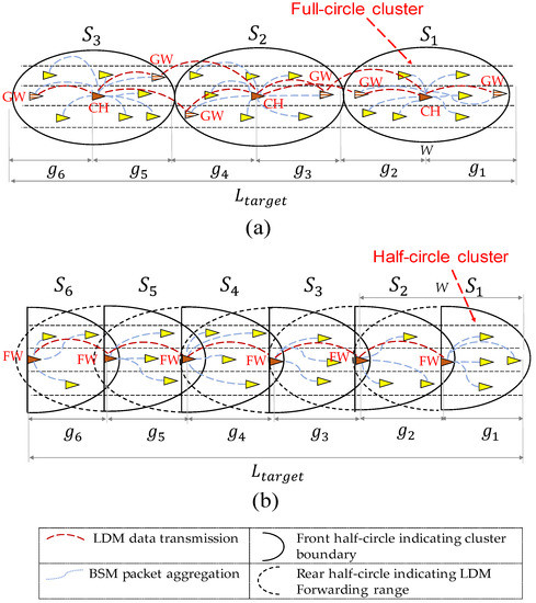
Figure 3. Cluster methods: (a) full-circle clustering method; (b) half-circle clustering method.

Additionally, in the full-circle clustering method, the LDM data of lagging clusters is unnecessarily propagated to the leading clusters. To increase the safety, each vehicle should know a recent mobility information of its leading neighbors. Thus, a forward propagation of LDM data is considered as an unnecessary procedure that generates a large redundant data.

In the proposed clustering method shown in Figure 3b, we elect one forwarder (FW) from each cluster to act as both the CH and the GW node. Then, we group all one-hop leading neighbors of FW into one cluster as shown in Figure 3b. The FW aggregates all BSM packets received from its one-hop leading neighbors. Then, it forwards this aggregated data to the lagging cluster which is a set of one-hop lagging neighbors of that FW. Although the leading FWs receive the aggregated LDM from their lagging FWs, they do not propagate this data to the leading clusters. As all one-hop neighbors of the FW are divided into two different clusters, we name our proposed scheme the half-circle clustering method.

There are two significant benefits of using the half-circle clustering scheme over the full-circle clustering method. Firstly, each FW can support direct communication with neighbor (leading and lagging) FWs. Therefore, each FW can maintain both intra-cluster and inter-cluster links, as shown in Figure 3b. Secondly, the half-circle clustering method allows FWs to transmit a redundant data much less than the full-circle clustering method. In the half-circle clustering scheme, LDM data is propagated only backward, and therefore data overhead is significantly reduced.

To have a fair comparison, let us assume that in both clustering methods the LDM data of cluster $S_i$ is propagated only backward upto target distance $L_{target}$ as shown Figure 3. In order to complete this mission, in both clustering schemes, the LDM packet of $S_i$ should be transmitted through $h$ hops. Then, this target distance is divided into multiple road segments $g_1,\dots ,g_n$, each of which represents the length of hop, as shown in Figure 3. In each $g_i$, there are $u_i$ number of nodes. Let $T_{Info}$ denotes a time it takes to transmit a mobility information of member vehicle ${\mathrm{v}}_i$ with a given link layer data rate. Since cluster $S_i$ contains $u_i$ nodes, it takes $u_i\times T_{Info}$ time to transmit LDM data of single cluster $S_i$. As transmission of redundant data degrades the channel efficiency, in following paragraphs, we demonstrate how our clustering method can reduce the time to transmit the redundant data while constructing the multi-hop LDM. We define this time as communication overhead.

In Figure 3, $g_1$, $g_2$, $g_3$, $g_4$, $g_5$, and $g_6$ represent six different road segments each of which contains $u_1$, $u_2$, $u_3$, $u_4$, $u_5$, and $u_6$ nodes respectively. In this example, the number of hops $h$ is 5. Let us assume that there is no cluster in front of $S_1$. Then, in full-circle clustering method, a total time $T_{FCC}$ it takes to transmit the aggregated LDM packet upto $L_{target}$ distance is given as:

The time required to transmit LDM data in each hop is:

$$t_{1sthop}=\left(u_1+u_2\right)\times T_{Info}$$

which is CH-1’s collection time for $u_1$ messages from segment $g_1$ and $u_2$ messages from segment $g_2$.

$$t_{2ndhop}=\left(u_1+u_2\right)\times T_{Info}$$

which indicates the transmission time for CH-1 to forward its LDM to GW-1

$$t_{3rdhop}=\left(u_1+u_2+u_3+u_4\right)\times T_{Info}$$

which is the sum of transmission time for GW-1 and collection time for $u_3$ and $u_4$

$$t_{4thhop}=\left(u_1+u_2+u_3+u_4\right)\times T_{Info}$$

which is the transmission time for CH-2 to forward its LDM to GW-2

$$t_{5thhop}=\left(u_1+u_2+u_3+u_4+u_5+u_6\right)\times T_{Info}$$

which is the sum of transmission time for GW-2 and collection time for $u_5$ and $u_6$.

Finally, the total time required to transmit all messages to construct and forward the LDMs to 5 hops in Figure 3a is

$$T_{FCC}=T_{Info}\left(2\times {\displaystyle \sum }_{i=1}^2{u}_i+2\times {\displaystyle \sum }_{i=1}^4{u}_i+{\displaystyle \sum }_{i=1}^6{u}_i\right)$$

In contrast, for the half-circle clustering method, the transmission time consumed by each hop is

$$t_{1sthop}=u_1\times T_{Info}$$

which is FW-1’s collection time for $u_1$ messages from segment $g_1$.

$$t_{2ndhop}=\left(u_1+u_2\right)\times T_{Info}$$

which is the sum of FW-2’s collection time for $u_2$ messages and LDM message from FW-1.

$$t_{3rdhop}=\left(u_1+u_2+u_3\right)\times T_{Info}$$

which is the sum of FW-3’s collection time for $u_3$ messages and LDM message from FW-2.

$$t_{4thhop}=\left(u_1+u_2+u_3+u_4\right)\times T_{Info}$$

which is the sum of FW-4’s collection time for $u_4$ messages and LDM message from FW-3.

$$t_{5thhop}=\left(u_1+u_2+u_3+u_4+u_5\right)\times T_{Info}$$

which is the sum of FW-5’s collection time for $u_5$ messages and LDM message from FW4.

The following equation gives the total transmission time $T_{HCC}$ including all BSM messages and LDM messages for the five hops in Figure 3b

$$T_{HCC}=T_{Info}\left(u_i+{\displaystyle \sum }_{i=1}^2{u}_i+{\displaystyle \sum }_{i=1}^3{u}_i+{\displaystyle \sum }_{i=1}^4{u}_i+{\displaystyle \sum }_{i=1}^5{u}_i\right)$$

while the half-circle method transmits only minimum messages needed to finish forwarding LDMs over five hops, the full-circle method transmits redundant messages repeatedly. For example, redundant messages of $u_2$, $u_4$, and $u_6$ vehicles are retransmitted a substantial overhead that can be reduced by the half-circle method. In half-circle clustering, the messages from $u_6$ are not transmitted since they have already been collected by the last forwarder.

To simplify the formula without loss of generality, suppose that the number of nodes in each cluster is $u_{avg}$, the average number of nodes per cluster. This is an acceptable assumption, since in a high density scenario, the number of nodes in each cluster can be bounded with the maximum allowable number of nodes, $u_{max}$. By substituting $T_{u_{avg}}$ for $u_{avg}\times T_{Info}$, $T_{FCC}$, and $T_{HCC}$ for Figure 3 can be generalized as functions of only the number of hops (h), respectively

$$\begin{gathered} T_{FCC}\left(h\right)=T_{u_{avg}}[2h+2\left(h-2\right)+2\left(h-4\right)] \\ {T}_{HCC}\left(h\right)=T_{u_{avg}}\left[h+\left(h-1\right)+\left(h-2\right)+\left(h-3\right)+\left(h-4\right)\right] \end{gathered}$$

Lemma 1:

Given a very large h, a reduction of communication overhead, $T_{FCC}-T_{HCC}$, approaches$T_{u_{avg}}\times \frac{h}{2}$.

Proof:

The transmission time $T_{FCC}$ and $T_{HCC}$ with a large h can be represented by the series functions of $h$. These series functions are expressed by Equations (1) and (2).

$$T_{FCC}\left(h\right)=T_{u_{avg}}\times 2\left[h+\left(h-2\right)+\left(h-4\right)+\dots \right]\cong T_{u_{avg}}\left(\frac{h^2}{2}+h\right)$$

(1)

$$T_{HCC}\left(h\right)=T_{u_{avg}}\left[h+\left(h-1\right)+\left(h-2\right)+\dots \right]=T_{u_{avg}}\frac{h\left(h+1\right)}{2}$$

(2)

Equation (1) can be reduced to $T_{u_{avg}}\left(\frac{h^2}{2}+h\right)$, while Equation (2) can be reduced to $T_{u_{avg}}\left(\frac{h^2}{2}+\frac{h}{2}\right)$. Therefore, $T_{FCC}-T_{HCC}$ approaches $T_{u_{avg}}\times \frac{h}{2}$ for a large h.

This proves that the proposed half-circle clustering method can reduce the communication overhead by $T_{u_{avg}}\times \frac{h}{2}$ compared with the conventional full-circle clustering method. □

Figure 4 compares the communication overhead of the two methods for initial 10 hops. In the proposed method, clusters utilize different transmit windows to perform communication. Neighboring clusters are assigned with different windows, while clusters in far distance may reuse the same window.

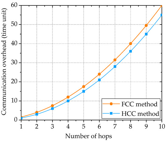
Figure 4. Communication overhead in full-circle and half-circle clustering.

5. Forwarder Election Algorithm

5.1. Problem Definition

To provide efficient and reliable LDM data dissemination, we propose a geographically optimized clustering topology. Within each cluster, we use a star topology for one-hop data aggregation. This topology requires one forwarder to cover the entire cluster population. In addition, to ensure channel resource allocation to all cluster members, we constrain the cluster size by $u_{max}$, the maximum allowable number of nodes as defined in Section 4.

For a target vehicular network, we construct a set of half-circle clusters (described in Section 4) by electing a set of forwarders. The forwarders are elected in a way that keeps the forwarders separated by a maximal distance called the ‘inter-forwarder gap’. By maximizing the inter-forwarder gaps, the objective of our forwarder election algorithm is to minimize the number of clusters in the target network, reduce inter-cluster interference, and maximize the channel utilization.

Let $\left\{F_1,\dots ,F_n\right\}$ be a set of total possible forwarders in the network. We denote $G_{Total}$ as a set of gaps between these forwarders $G_{Total}=\left\{g_1,\dots ,g_{n-1}\right\}$ where each $g_i$ represents the distance between $F_i$ and $F_{i+1}$. The number of nodes in cluster $S_i$ is denoted by $u_i$ while $W$ indicates the wireless transmission range of V2X devices. For simplicity, we assume that $W$ is identical in all clusters. Then, we define the objective and constraints for the forwarder election algorithm as follows:

• Objective: ${\mathrm{Maximize}}_{i\in \left[1\dots n-1\right]}{g}_i$
• Constraint 1: For each $u_i$, $u_i\le u_{max}$.
• Constraint 2: For all $g_i\in G_{Total}$, $g_i<W$

In the remainder of this section, we present the procedure and performance of the forwarder election algorithm.

5.2. Forwarder Election

The proposed forwarder election algorithm is described in the following steps using a multilane highway network of Figure 5. In this network, each vehicle can initiate forwarder election procedure at random time. In this procedure, vehicle can elect itself as forwarder and broadcast a forwarder designation message $M_{FDM}$. A vehicle broadcasts $M_{FDM}$ message in the following two cases:

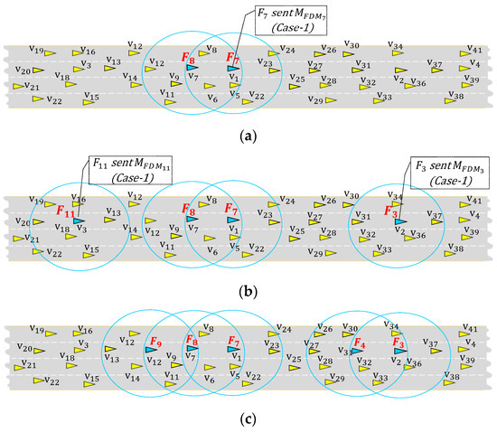
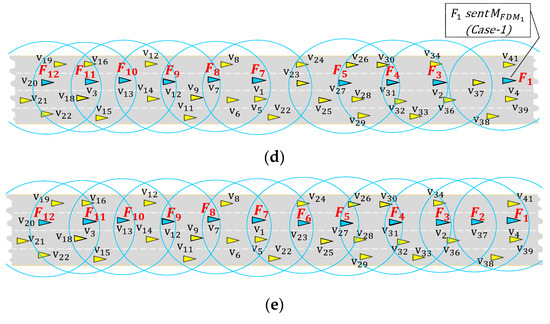
Figure 5. Forwarder election procedures in the proposed method. (a) initial forwarder is elected by Case 1; (b) the forwarders are simultaneously elected by Case 1 and Case 2; (c) the forwarders $F_9$ and $F_{12}$ are elected by Case 2; (d) the forwarders $F_{10}$ and $F_5$ are elected by Case 2 while $F_1$ is elected by Case 1; (e) the vehicles on highway road is divided into 12 different clusters.

• Case 1: When the current vehicle ${\mathrm{v}}_{HV}$ is a new vehicle with no leading forwarder, ${\mathrm{v}}_{HV}$ schedules a transmission of $M_{FDM}$ in randomly selected slot.
• Case 2: When ${\mathrm{v}}_{HV}$ has a leading forwarder, ${\mathrm{v}}_{HV}$ schedules a transmission of $M_{FDM}$ using a distance-based back-off timer.

In Algorithm 1, we summarize the basic steps of the distributed forwarder election procedure. While running Algorithm 1 in each vehicle, when it elects itself as a forwarder, it broadcasts $M_{FDM}$, under the Case1 and Case2 conditions.

Algorithm 1Distributed forwarder election algorithm

Input:${\mathrm{v}}_{HV}$ is host vehicle, $M_{FDM}$ is forwarder designation message, $t_{DB}$ is distance-based back-off timer,$t_{FR}$ is forwarder re-election timer Output: leading forwarder $F_{Lead}$, lagging forwarder $F_{Lag}$ 1 loop 2  //Case1: 3   if ${\mathrm{v}}_{HV}$ is new vehicle (with no $F_{Lead}$ in the neighbor) 4     if $M_{FDM}$ is not scheduled for ${\mathrm{v}}_{HV}$ then 5       Schedule $M_{FDM}$ in random slot from $\left[0,N_{FD}-1\right]$ 6      else if time reaches selected slot then 7       Elect itself as forwarder and broadcast $M_{FDM}$ 8      end if 9   //Case2: 10    else if ${\mathrm{v}}_{HV}$ receives $M_{FDM}$ from $F_{Lead}$ or $F_{Lag}$ then 11     Record ID of $F_{Lead}$ or $F_{Lag}$//forwarder that sent $M_{FDM}$ 12     Dismiss its own $M_{FDM}$, if it was scheduled 13     if $F_{Lag}$ is undefined then 14      Schedule $M_{FDM}$ with back off timer of $t_{DB}$ using Equation (3) 15     end if 16    end if 17    Decrement the back off timer 18    if $t_{DB}$ timer expires then//$t_{DB}$ is defined and $F_{Lag}$ is unknown 19     ${\mathrm{v}}_{\mathrm{HV}}$ elects itself $F_{Lag}$ and sends ${\mathrm{M}}_{\mathrm{FDM}}$ 20   end if 21  end loop

Case 1: (Algorithm 1 line 2–8) Using a contention window method like CSMA protocol, each vehicle randomly selects a time slot to transmit its $M_{FDM}$ message. We allocate a short contention time window for $M_{FDM}$ transmission. We partition the contention window into $N_{FD}$ slots of time length $t_s$. Then, each vehicle ${\mathrm{v}}_i$ selects a random slot from [$0,N_{FD}-1]$. Then, ${\mathrm{v}}_i$ schedules its message $M_{FDM}$ to be sent in the selected slot.

If ${\mathrm{v}}_i$ selected earlier slot than other neighbors, ${\mathrm{v}}_i$ transmits $M_{FDM}$ in its slot and then becomes forwarder $F_i$. On the other hand, if ${\mathrm{v}}_i$ selects later slot, other vehicle would transmit its $M_{FDM}$ and become a forwarder. If ${\mathrm{v}}_i$ receives $M_{FDM}$ from other vehicle, it dismisses its own transmission scheduled at randomly selected slot. For example, Figure 5a,b,d show examples of initial forwarders elected in this way (${\mathrm{v}}_1$, ${\mathrm{v}}_2$, ${\mathrm{v}}_3$, and ${\mathrm{v}}_4$ select themselves as $F_7$, $F_3$, $F_{11}$, and $F_1$ that selected the earliest time slots).

Lines 3–8 of Algorithm 1 describe Case-1, where a new vehicle ${\mathrm{v}}_{HV}$ which has no neighbor forwarder selects a random back off slot. Then, ${\mathrm{v}}_{HV}$ schedules a transmission of $M_{FD{M}_{HV}}$ at selected slot in line 5 and decrements its back off timer.

Case 2: (Algorithm 1 line 9–20) The elected forwarders are denoted either by $F_{Lead}$ or $F_{Lag}$. Here, the order of forwarders is opposite to traveling direction of vehicles. In other words, $F_{Lead}$ denotes the previous forwarder for the leading cluster from the perspective of the current forwarder, while $F_{Lag}$ is the next forwarder for the lagging cluster. For example, in Figure 5b, ${\mathrm{v}}_1$ is $F_{Lead}$ of ${\mathrm{v}}_7$, while ${\mathrm{v}}_7$ is $F_{Lag}$ of ${\mathrm{v}}_1$. In Case2, the algorithm elects the lagging forwarder $F_{Lag}$ only with respect to its previous forwarder $F_{Lead}$ (backward of the vehicle travel direction).

The $M_{FDM}$ message received from $F_{Lead}$ initiates a forwarder election procedure which elects a $F_{Lag}$ among the neighbors that are one-hop lagging from $F_{Lead}$. Our proposed algorithm uses a technique called a distance-based back-off procedure to elect $F_{Lag}$. Each lagging neighbor represented as a host vehicle ${\mathrm{v}}_{HV}$ computes its distance-based back-off timer $t_{DB}$ using Equation (3).

$$t_{DB}=\left[\frac{W-Dist\left(Locatio{n}_{HV}\left(t\right),Locatio{n}_{F_{Lead}}\left(t\right)\right)}{W}\right]\times t_s$$

(3)

Here, $Locatio{n}_{HV}\left(t\right)$ denotes the location of host vehicle at $t$ time. Similarly, $Locatio{n}_{F_{Lead}}\left(t\right)$ is the location of $F_{Lead}$ (the forwarder of the previous cluster of ${\mathrm{v}}_{HV}$) at time $t$. The algorithm elects as $F_{Lag}$ the neighbor ${\mathrm{v}}_{HV}$ that has the shortest $t_{DB}$ or the farthest inter-vehicle distance from $F_{Lead}$. The $t_{DB}$ of ${\mathrm{v}}_{HV}$ constantly decrements until it expires. Once $t_{DB}$ of ${\mathrm{v}}_{HV}$ expires, ${\mathrm{v}}_{HV}$ elects itself as a forwarder, and broadcasts $M_{FD{M}_{HV}}$ to notify all one-hop neighbors. Then, all receivers located in front of ${\mathrm{v}}_{HV}$’s wireless range become the member of current cluster, where ${\mathrm{v}}_{HV}$ is self-designated forwarder. For example, in Figure 5a, $M_{FDM}$ from $F_7$ (current $F_{Lead}$) initiates distance-based back-off procedures in the lagging neighbors ${\mathrm{v}}_6$, ${\mathrm{v}}_7$, and ${\mathrm{v}}_8$. From Equation (3), $t_{D{B}_7}<t_{D{B}_8}<t_{D{B}_6}$, since the distance from $F_7$ is the farthest from ${\mathrm{v}}_7$, and closest from ${\mathrm{v}}_6$. Since $t_{D{B}_7}$ decrements to zero before $t_{D{B}_8}$ and $t_{D{B}_6}$, ${\mathrm{v}}_7$ declares itself as the next forwarder $F_8$ (an $F_{Lag}$ of the current $F_{Lead}$). This procedure is repeated by $F_8$ acting as a next $F_{Lead}$ to elect the next $F_{Lag}$.

In this way, all forwarders are elected, and all vehicles are connected through the elected forwarders as shown in Figure 5e. The current positions of the forwarders, however, may not be optimal, since initial forwarders are randomly elected, and vehicles continuously change their locations. To maximize the gaps between these forwarders, Algorithm 1 iteratively runs the forwarder re-election operation to find better forwarder positions. The forwarder re-election is an iterative procedure (executed every forwarder re-election cycle), which strives to discover the optimum forwarders in the continuously changing vehicular network. The re-election procedure is conducted by Case 2 in Algorithm 1 by repeatedly sending $M_{FDM}$ with random back off timer to initiate election of optimal lagging forwarder. The forwarder re-election procedure is conducted from front to backward.

Each forwarder $F_{Lead}$ selects a random back off slot from $\left[0,N_{FR}-1\right]$ and transmits message $M_{FDM}$ to elect a new $F_{Lag}$. Each lagging vehicle ${\mathrm{v}}_i$ that receive $M_{FDM}$ verifies following two conditions:

(a)

$d_{th}\le \left(Dist\left(F_{Lead},{\mathrm{v}}_i\right)-Dist\left(F_{Lead},F_{Lag}\right)\right)$, where $d_{th}$ is a threshold distance which triggers distance-based back off procedure for ${\mathrm{v}}_i$.

(b)

$u_i\le u_{max}$, where $u_i$ is the number of nodes located between $F_{Lead}$ and ${\mathrm{v}}_i$.

Condition (a) avoid too frequent changes of forwarders, while condition (b) ensures that the cluster for $F_{Lead}$ does not exceed $u_{max}$, the maximum number of vehicles.

If ${\mathrm{v}}_i$ satisfies above two conditions, then it can contend to be $F_{Lag}$ by scheduling its $M_{FDM}$ at the back off slot based on Equation (3). The ${\mathrm{v}}_i$ that has the shortest back-off timer is re-elected as a new $F_{Lag}$, and sends $M_{FDM}$ to announce itself as a new lagging forwarder.

Figure 6 illustrates an example of re-election, $F_6$ sends $M_{FD{M}_6}$ to its lagging vehicles and initiates the re-election procedure. Since ${\mathrm{v}}_5$ is the farthest node from $F_6$, ${\mathrm{v}}_5$ sends $M_{FD{M}_5}$ with the shortest timer $t_{D{B}_5}$, before other vehicles announce themselves as a new $F_7$. Upon receiving $M_{FD{M}_5}$ from ${\mathrm{v}}_5$, ${\mathrm{v}}_{24}$, ${\mathrm{v}}_{22}$, and ${\mathrm{v}}_1$ cancel their distance-based back-off procedure. ${\mathrm{v}}_1$ changes its status from forwarder to a member vehicle. This procedure is iteratively done by each forwarder to maximize the inter-forwarder gap.

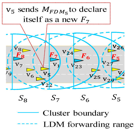
Figure 6. Forwarder re-election procedure.

5.3. Analysis of Time Complexity

In this subsection, we analyze the upper bound time complexity of forwarder re-election procedure. For simplicity, we assume that all clusters (vehicles) are stationary within time interval $\left[t_1,t_2\right]$. Figure 7 shows $n$ forwarders indexed in ascending order from the right to the left. For the sake of simplicity, let us assume that it takes constant $t_{elct}$ time to announce a new forwarder in every re-election operation. Then, let is define a set of forwarders as $\left\{F_1,F_2,\dots ,F_n\right\}$ where $F_k$ and $F_{k+1}$ is separated by gap $g_k$. A set of gaps between each pair of the forwarders is denoted by $\left\{g_1,g_2,\dots ,g_{n-1}\right\}$ as shown in Figure 7. In the worst case scenario, if any $F_k$ starts re-election operation at random $t_i$, it causes $n-k$ recursive re-election operations where each inter-forwarder gap $g_k$ changes to $g_k^{\text{’}}$ (maximum distance). Then, the time required to run $n-k$ recursive re-election operations can be expressed by a time function $f\left(k\right)$ (see that in Figure 8a).

$$f\left(k\right)=\left(n-k\right)\times t_{elct}$$

Figure 7. Forwarders in one-dimensional space separated by initial inter-cluster gaps.

Figure 8. Recursive relation of forwarder re-election procedures: (a) recursive re-election for $k$ clusters; (b) recursive re-election for $m$ clusters.

Let $F_m$ be the next forwarder that launches re-election at $t_{i+1}$. Then, $F_m$ triggers $n-m$ recursive re-election operations as shown in Figure 8b. Since $F_m$ leads $F_k$, $n-k$ forwarders run re-election operation again. Then, the time it takes for $n-m$ forwarders to complete re-election procedure becomes

$$f\left(m\right)=\left(n-m\right)\times t_{elct}=\left[\left(n-k\right)+\left(k-m\right)\right]\times t_{elct}$$

Considering this recursive relation, we define the following lemma.

Lemma 2:

Let$\left\{g_1,g_2,\dots ,g_{n-1}\right\}$be a set of inter-forwarder gaps for n forwarders. Then, each $g_i$converges to the maximum gap after iterative forwarder re-election procedures conducted within the time bound$O\left(n^2\right)$.

Proof:

As described above, in the worst case, the forwarder re-election procedure repeatedly conducted by each forwarder from $F_{n-1}$ to $F_1$ in $n-1$ iterations, which can be written as:

$$\begin{gathered} f\left(n\right)=0\times t_{elct} \\ f\left(n-1\right)=1\times t_{elct} \\ f\left(n-2\right)=2\times t_{elct} \\ ⋮ \\ f\left(2\right)=\left(n-2\right)\times t_{elct} \\ f\left(1\right)=\left(n-1\right)\times t_{elct} \end{gathered}$$

Note that the re-election time for $F_n$ is zero, since $F_n$ is the last forwarder. Then, the total time it takes to maximize all $\left(n-1\right)$ inter-forwarder gaps in the worst case is the sum of all recursive re-election time $f\left(n-1\right)$,$f\left(n-2\right)$, …, $f\left(1\right)$. We denote a total time as $T\left(n\right)$.

$$T\left(n\right)=f\left(n\right)+f\left(n-1\right)+f\left(n-2\right)+\dots +f\left(2\right)+f\left(1\right)=\left[0+1+\dots +\left(n-2\right)+\left(n-1\right)\right]\times t_{elct}$$

(4)

By reversing the ordering, Equation (4) can be expressed by Equation (5).

$$T\left(n\right)=\left[\left(n-1\right)+\left(n-2\right)+\dots +1+0\right]\times t_{elct}$$

(5)

Then, adding Equation (4) with Equation (5) produces Equation (6).

$$2T\left(n\right)=\left[\left(n-1+0\right)+\left(n-2+1\right)+\dots +\left(1+n-2\right)+\left(0+n-1\right)\right]\times t_{elct}$$

(6)

Then, Equation (6) is represented by $\left[n\times \left(n-1\right)\right]\times t_{elct}$ which leads to Equation (7).

$$T\left(n\right)=\frac{n^2-n}{2}\times t_{elct}$$

(7)

The Equation (7) proves that the proposed algorithm takes $O\left(n^2\right)$ time to maximize each of $\left\{g_1,g_2,\dots ,g_{n-1}\right\}$. □

The overall processing time of the proposed algorithm is dominated by the recursive re-election time, since the initial election time is given by $n\times t_{elct}$, which is negligible. This proves that the proposed forwarder election algorithm can obtain optimal result in complexity of $O\left(n^2\right)$ even in the worst case.

6. Transmit Window Allocation

This section describes the transmit window allocation algorithm based on coloring to maximize the channel utilization. Figure 9 illustrates an example of cluster coloring on a road segment with four clusters, each of which selects one color out of predefined set $\left\{C_1,\dots ,C_{N_C}\right\}$. We partition the transmission interval $T_b$ into $N_C$ of short transmit windows, which is represented as $\left\{T_1,\dots ,T_{N_C}\right\}$. Then, each transmit window $T_i$ corresponds to predefined color $C_i$. If forwarder $F_k$ of cluster $S_k$ selects a window $T_i$, then all member vehicles in $S_k$ transmit their BSM packet and $F_k$ forwards the LDM message within $T_i$ window. For example, Figure 9 illustrates a case of using three colors (red, green, blue), each of which indicates unique transmit window ($T_1$, $T_2$, and $T_3$). All vehicles in each cluster transmit messages only within allocated transmit window, while they receive messages all time. However, one transmit window can be reused by multiple clusters if the distance between these clusters is large enough, so their vehicles do not interfere. In Figure 9, vehicles in two different clusters $S_i$ and $S_m$ are colored red. This means the members of these clusters access the channel within $T_1$ of $T_b$. The forwarder $F_i$ then receives all the packets sent by the member vehicles of $S_i$ as indicated by the solid half circle around $F_i$. Then, it aggregates these packets to create the LDM data of $S_i$. Then, $F_i$ forwards the LDM data to the cluster behind $S_j$. In the same way, $F_j$ also creates the LDM data of $S_j$ and aggregates it with the LDM data received from $F_i$. Then, $F_j$ sends its aggregated LDM data to cluster $S_k$. Following the same procedure, $F_k$ also builds the LDM data of $S_k$ and adds it to the aggregated data received from $F_j$. Next, $F_k$ transmits its aggregated LDM data to cluster $S_m$. In this way, the LDM data of  reaches vehicles in cluster $S_k$ through a multihop forwarding procedure indicated with dashed half circle of Figure 9. When $F_i$ transmits its LDM data to $F_j$, $F_h$ also receives the LDM data of $F_i$ since it is sent as a broadcast packet. Then, $F_h$ verifies whether its LDM data is successfully received and aggregated in the LDM packet of $F_i$.

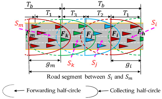
Figure 9. Cluster coloring in a segment of road where identical color is used by two different clusters.

To color each cluster, we allocate a predefined contention period. This contention period is divided into $N_{CD}$ slots of time length $t_s$. Each forwarder select a random slot out of [$0,N_{CD}-1$] to declare its selected color. Algorithm 2 describes the basic steps of distributed color selection procedure. Algorithm 2 starts by checking whether the host vehicle ${\mathrm{v}}_{HV}$ is a forwarder or not (line 2). If ${\mathrm{v}}_{HV}$ is a forwarder, then ${\mathrm{v}}_{HV}$ verifies whether it has selected its own color (line 3). If color is undefined, ${\mathrm{v}}_{HV}$ picks a random slot in which it declares its selected color (line 4). Meanwhile, in line 11–13, if ${\mathrm{v}}_{HV}$ receives color from a neighbor forwarder $F_{Nbr}$, then ${\mathrm{v}}_{HV}$ records this color in a local color table denoted as $Tabl{e}_{Col}$ (later this table is shared with neighboring clusters). In Figure 9, let us assume that $F_i$ selects an earlier slot than $F_j$. Then, $F_j$ receives color information from $F_i$ before $F_j$ picks its color, and, $F_j$ records the color of $F_i$ in $Tabl{e}_{Co{l}_j}$. Then, in the later slot, $F_j$ transmits its selected color with its updated $Tabl{e}_{co{l}_j}$. When $Tabl{e}_{co{l}_j}$ is received by $F_i$, $F_i$ verifies whether its coloring details are recorded in $Tabl{e}_{co{l}_j}$. If it is not recorded, then $F_i$ concludes that there has happened when it transmitted its coloring details. Therefore, $F_i$ selects another random slot to re-announce its selected color.

Algorithm 2 Distributed color selection algorithm
Input:$F_{Nbr}$ is neighbor forwarder, $Tabl{e}_{Col}$ is a table that contains color information received from $F_{Nbr}$’s
Output: color (transmit window)
1 2 3 4 5 6 7 8 9 10 11 12 13 14 15 16 17 18 19	Loop  if${\mathrm{v}}_{HV}$ is forwarder then//for forwarders if Color is undefined then     if Color designation slot is undefined then Select a random slot from $\left[0,N_{CD}-1\right]$ else if time reaches selected slot then      Select minimum cost color using Equation (8)//pick window      Broadcast coloring information//declare Tx Window end if end if if Color designation message is received from $F_{Nbr}$ then Insert $F_{Nbr}$’s coloring details in $Tabl{e}_{Col}$ end if  else//for member vehicles   if Color is received from forwarder then    Schedule BSM transmission within transmit window corresponds to received color   end if  end if end loop

In line 6 of Algorithm 2, once time reaches the selected slot of ${\mathrm{v}}_{HV}$, ${\mathrm{v}}_{HV}$ runs line 7 to calculate the cost for each color and then select the one with minimum cost. Our cost calculation function relies on Friis free space propagation model [26]. This model is defined as $P_r\left(d\right)=P_{t}K{\left(d_0/d\right)}^2$, where a power of received signal $P_r$ is inversely proportional to the square of $d$, the distance between transmitter and receiver. $P_t$, $K$, and $d_0$ are constants representing transmission power, unitless coefficient, and reference distance, respectively [20]. Therefore, we disregard these constant parameters while defining the cost function in Equation (8). We use Cost(C_j) to denote aggregated cost of color $C_j$.

$$Cost\left(C_j\right)={\displaystyle \sum }_{F_{Nbr}\in Tabl{e}_{Col}}\frac{1}{Dist{\left({\mathrm{v}}_{HV},F_{Nbr}\right)}^2}$$

(8)

Here, $Dist\left({\mathrm{v}}_{HV},F_{Nbr}\right)$ is the function which calculates a distance between ${\mathrm{v}}_{HV}$ (considering ${\mathrm{v}}_{HV}$ as a forwarder of current cluster) and neighbor $F_{Nbr}$.

The cost of free color (not occupied by any $F_{Nbr}$) is zero, since the distance for free color represents infinite value in Equation (8). Once ${\mathrm{v}}_{HV}$ selects a minimum cost color, then ${\mathrm{v}}_{HV}$ broadcasts its color (and its color table) as shown in line 8 of Algorithm 2. In Figure 9, let us assume that $F_j$ is the next forwarder who selects color after $F_i$. Suppose that $F_j$ received color information: red color from $F_i$ and green color from $F_h$. Then, $F_j$ picks blue color from (red, green, blue), since blue is unoccupied color and thus gives zero cost. Suppose that $F_k$ is the next to select the color. Then, $F_k$ selects green color since red and blue colors have higher cost due to the shorter distance of their $F_{Nbr}$.

In case when ${\mathrm{v}}_{HV}$ is a member vehicle, it polls the color information of its forwarder. Once ${\mathrm{v}}_{HV}$ receives color from its forwarder, then ${\mathrm{v}}_{HV}$ schedules its BSM transmission within the transmit window corresponding to the forwarder’s color.

The proposed cluster coloring scheme can also be applied to grid structured crowded city roads with many intersections. To reduce the interference in the intersection area, we can extend $T_b$, the beaconing period, to accommodate more colors. Then, the additional colors can be assigned to the clusters representing the roads crossing with the main road at the intersection. This way, we can minimize the potential inter-cluster interference in the intersection area.

The increased number of colors may degrade the channel reuse efficiency. In other words, if we increase the number of colors, a distance between the interfering clusters becomes larger. On the other hand, if we use the minimum number of colors, more vehicles can transmit their BSM packet in the same transmit window. Therefore, we should use the minimum colors to maintain better channel reuse efficiency.

Requirement of Transmit Window

Each transmit window is divided into two sub-windows: (1) aggregation sub-window $T_{\mathrm{agg}}$ and (2) dissemination sub-window $T_{diss}$ as shown in Figure 10. The aggregation sub-window is defined as

$$T_{\mathrm{agg}}=u_{max}\times \left(T_{CSMA}+T_{BMS}\right)$$

(9)

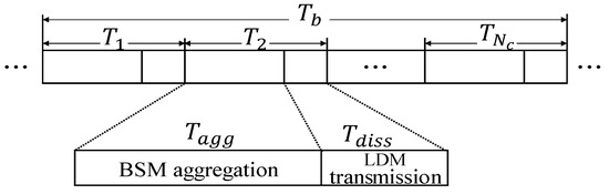
Figure 10. The allocation of time within the window.

Here, $T_{BSM}$ represents a time it takes to transmit single BSM packet while $T_{CSMA}$ is a maximum time required to access the channel using the standard carrier sense multiple access (CSMA) scheme. By multiplying $u_{max}$ (a maximum number of members in a cluster), Equation (9) represents the maximum required aggregation sub-window.

In Equation (10), we define dissemination sub-window in which the forwarder transmits its aggregated LDM packet to the next cluster.

$$T_{diss}=u_{max}\times h\times T_{Info}$$

(10)

Here, $T_{Info}$ is a time required to send mobility information of each ${\mathrm{v}}_i$, while $h$ is the number of hops indicating that the LDM of $h$ clusters is accumulated. By multiplying $u_{max}$, Equation (10) represents the upper limit of the LDM size. Equation (11) gives the maximum length of transmit window $T_i$.

$$T_i=T_{\mathrm{agg}}+T_{diss}=u_{max}\times \left(T_{BSM}+T_{CSMA}+h\times T_{Info}\right)$$

(11)

Since $N_c$ denotes the number of colors (transmit windows), we can identify $u_{max}$ for each cluster using Equation (12).

$$u_{max}=\frac{T_b}{N_C\times \left(T_{BSM}+h\times T_{Info}+T_{CSMA}\right)}$$

(12)

In Equation (12), we can see the parameters $N_C$ and $h$ are inversely proportional to $u_{max}$. We can observe the property that to increase $u_{max}$, $N_C$ should be reduced. In this paper, we use a fixed number of colors to disseminate the LDM data up to a fixed number of hops for simplicity.

7. Performance Evaluation

7.1. Simulation Set-Up

To evaluate our algorithm, we implemented it using NS3 simulator, and tested the performance with a highway mobility scenario. We configured the simulations with vehicles moving with random speed on a multilane highway road of 5 km. The speed of the vehicles varies in the range of 10–35 m/s. To simulate the communication between the vehicles, we used the NS3 library that supports the IEEE 1609 standard. Table 2 summarizes the parameters used in our simulation. We also implemented a previous method called CB-BDP [16] using NS3 and compared the performance of the two methods.

Table 2. Simulation settings

Specification	Value
Length of highway	5 km
MAC and PHY parameters	IEEE 802.11p
Data Rate	6 Mbps
Beacon frequency	10 Hz
Maximum velocity	35 mps
Average wireless range	250 m
Maximum number of members $u_{max}$	44
Target number of hops	5
Number of lanes	4
Simulation time	80 s

7.2. Results

In the proposed method, every forwarder collects the mobility information of all members and then aggregates this data into a single LDM packet. Then, it broadcasts the LDM packet within its dissemination sub-window. Figure 11 shows a reception ratio of the LDM packet for the member vehicles. The reception ratio for one transmitted LDM packet is calculated by X/Y, where Y is a number of expected receivers and X is the number of receivers with successful reception. We consider all the member vehicles within the wireless range of the forwarder as the expected receivers.

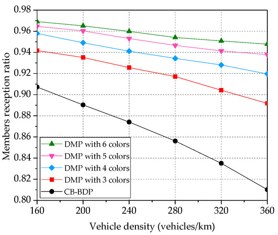
Figure 11. Impact of the number of colors on members reception ratio.

In this experiment, we proportionally extend the beaconing period $T_b$ to accommodate more colors (with each color representing each transmit windows). Therefore, in Figure 11, we also show the impact of increasing number of colors on a reception ratio of the member vehicles. The clusters are assigned with fixed wireless range and they may serve only $u_{max}$ vehicles. Therefore, when the vehicle density grows, the distance between the clusters with the identical color shrinks. Then, a communication conducted in one cluster may start interfering with the neighboring clusters. In such a case, the members’ reception ratio degrades if the number of available colors is not enough. DMP obtains a higher members’ reception ratio, when the number of colors increases. For example, DMP provides 17% improvement in members reception ratio over CB-BDP, when it utilizes six colors. This experiment also proves that DMP can be applied in crowded city area with many intersections. In an intersection, for example, the set of colors can be divided into multiple disjoint subsets and allocated to individual roads of the intersection to reduce the interference. Figure 12 shows a reception ratio of LDM message for the forwarders (forwarder to forwarder reception ratio).

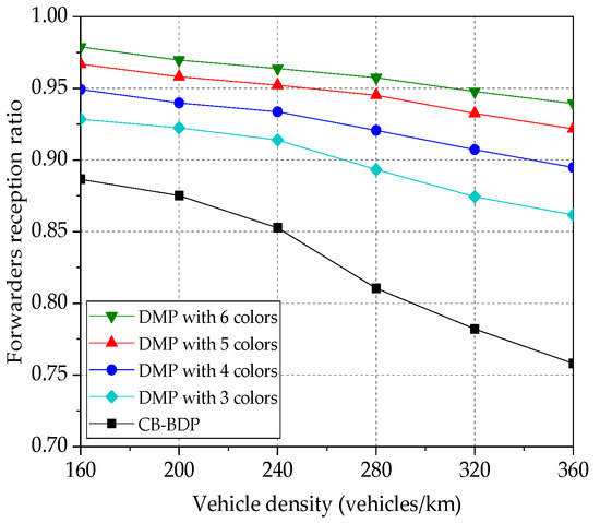
Figure 12. Impact of the number of colors on forwarders reception ratio.

When the vehicle density increases, the forwarders reception ratio decreases due to the inter-cluster interference. However, by increasing the number of colors, we can mitigate the interference and thus enhance the forwarders reception ratio. For example, when we increase the number of colors from 3 to 4, 5, and 6 colors, the forwarders reception ratio% gradually increases. By increasing the number of colors to 6, DMP improves the forwarders reception ratio by 20 compared to CB-BDP for a vehicle density of 360 vehicles/km. On the other hand, CB-BDP produces the worst results since it utilizes an inefficient way of data transmission from CH to CH. Each cluster head (CH) needs to select the gateways to forward its data to neighboring CH. For this communication, CB-BDP allocates common transmit window and thus, when we increase the density, it suffers more from the hidden terminal interference.

Figure 13 demonstrates the result of the experiment where the members reception ratio is measured for various network density. In this experiment, we change the forwarder re-election cycle time, in which re-election operation is periodically executed by each forwarder. Although a high network density causes reduction in the members reception ratio, a shorter re-election cycle improves the members reception ratio. For a vehicle density of 240 vehicles/km in Figure 13, when a re-election cycle of 1 s is chosen, the members reception ratio is 87.7%. When we shorten the re-election cycle to 0.5 s and 0.2 s, respectively, the members reception ratio increases to 90% and 91.8%.

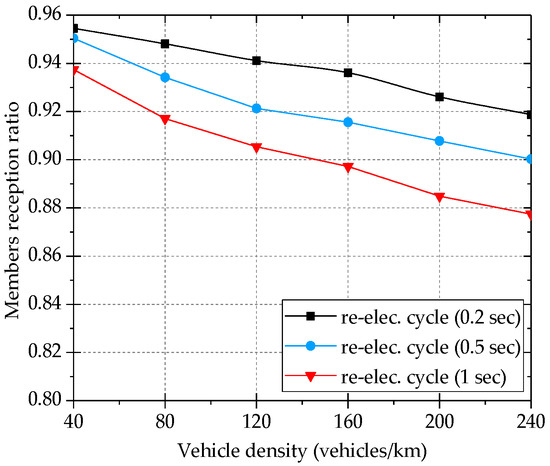
Figure 13. Impact of re-election cycle on members reception ratio.

Figure 14 compares the average propagation distance of LDM messages for the two algorithms. Since we constrain the number of member vehicles in each cluster by $u_{max}$, the cluster size (inter-forwarder gap) shrinks for the growing vehicle density. Thus, the LDM message dissemination distance decreases gradually as we increase the density. CB-BDP demonstrates a poor dissemination distance of 500 m for than DMP, since it suffers from a higher hidden terminal interference in the inter-cluster communication. For example, for a vehicle density of 360 vehicle/km in Figure 14, CB-BDP disseminates LDM only to 500 m, whereas DMP disseminates LDM up to 711 m (29% improvement).

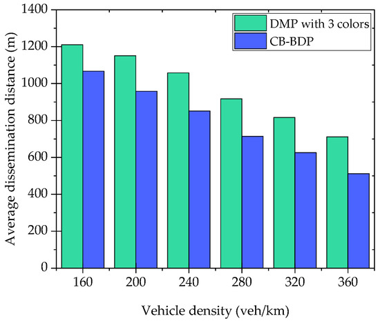
Figure 14. Average LDM message dissemination distance vs. vehicle density (number of target hops is 5).

As described in Section 5, we limit the cluster size by $u_{max}$ in order to ensure that all members of the cluster can transmit within the fixed transmit window. The number of colors is 3. The length of aggregation and dissemination sub-windows are 22 ms and 11 ms respectively. In this experiment, we aim to propagate the LDM within 200 ms latency constraint. Figure 15 presents impact of $u_{max}$ on the average LDM dissemination distance. We obtain the average LDM dissemination distance for three different $u_{max}$ of 30, 40, and 50. In all three cases, the LDM is disseminated up to the same predefined number of hops. For the $u_{max}$ of 50, we observed the largest dissemination distance. It means when we provide greater $u_{max}$ value, the clusters maintain longer inter-cluster distance. Therefore, each hop may represent relatively larger distance. The shortest dissemination distance is observed for a $u_{max}$ of 30. Since the clusters are allowed to have only 30 vehicles as the members, the size of clusters shrinks for the growing density. Overall, in the highest vehicle density, we achieve the average dissemination distances 514, 689, and 802 m for $u_{max}$ of 30, 40, and 50 respectively.

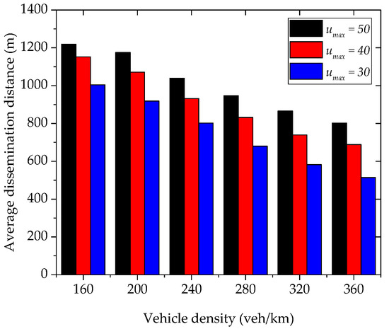
Figure 15. Impact of $u_{max}$ on the LDM dissemination distance (number of target hops is 5).

The above extensive simulation experiments demonstrated that DMP can offer substantial enhancement in the members reception ratio, forwarders’ reception ratio, and inter-forwarder distance compared with the previous method, CB-BDP.

8. Conclusions and Future Work

In this paper, we have proposed a local dynamic map propagation technique—dynamic map propagation (DMP) for clustered vehicular network. DMP uses the half-circle clustering method to reduce communication overhead during the inter-cluster communication. The proposed low-cost and distributed forwarder election algorithm dynamically identifies the forwarders and optimizes inter-forwarder gaps. To achieve efficient and reliable local dynamic map propagation, we exploit a distributed cluster coloring technique. The clusters utilize different transmit windows to minimize inter-cluster interference. Neighboring clusters are assigned with different transmit windows, while clusters with farther distances reuse the same transmit window. We evaluated the performance of DMP in comparison with cluster-based beacon dissemination process (CB-BDP), a previous full-circle clustering method. The simulation results demonstrated that DMP outperforms in all aspects of metrics evaluated. In the future, we plan to exploit this method in a 2D city environment.

In the future, we plan to extend the proposed clustering-based multi-hop LDM data propagation scheme to C-V2X and NR V2X networks. Using a multi-hop LDM data, we can realize interference-free resource allocation in two-dimensional time-frequency resource map. We also plan to apply deep reinforcement learning methods to optimize cooperative sensing and competitive resource selection for C-V2X.

References

- Intelligent Transport Systems (ITS). Decentralized Congestion Control Mechanisms for Intelligent Transport Systems Operating in the 5 GHz Range; Access Layer Part. 2018. Available online: https://www.etsi.org/deliver/etsi_ts/102600_102699/102687/01.02.01_60/ts_102687v010201p.pdf (accessed on 16 October 2020).
- IEEE. IEEE Standard for Wireless Access in Vehicular Environment (WAVE), IEEE Vehicular Technology Society Supported by the Intelligent Transmission Systems Committee, Revised Draft; IEEE: New York, NY, USA, 2014. [Google Scholar]
- Federal Motor Vehicle Safety Standards; V2V Communications. Department of Transportation, National Highway Traffic Safety Administration 49 CFR Part 571 [Docket No. NHTSA-2016-0126] RIN 2127-AL55; Proposed Rules; National Highway Traffic Safety Administration: Washington, DC, USA, 2016. [Google Scholar]
- Intelligent Transport Systems (ITS); Vehicular Communications; Basic Set of Applications; Local Dynamic Map (LDM); Rationale for and Guidance on Standardization. ETSI TR 102 863 V1.1.1 (2011-06); ETSI: Sophia-Antipolis, France, 2011. [Google Scholar]
- Annual Road Crash Statistics of Association of Safe International Road Travel. Available online: https://www.asirt.org/safe-travel/road-safety-facts/ (accessed on 16 October 2020).
- SAE International Standard. Dedicated Short-Range Communications (DSRC) Message Set Dictionary; J2735_200911; SAE: Warrendale, PA, USA, 2009. [Google Scholar]
- Jalooli, A.; Song, M.; Wang, W. Message coverage maximization in infrastructure-based urban vehicular networks. Veh. Commun. 2019, 16, 1–14. [Google Scholar] [CrossRef]
- Xue, L.; Yang, Y.; Dong, D. Roadside Infrastructure Planning Scheme for the Urban Vehicular Networks. Transp. Res. Procedia 2017, 25, 1380–1396. [Google Scholar] [CrossRef]
- Eiter, T.; Füreder, H.; Kasslatter, F.; Parreira, J.X.; Schneider, P. Towards a Semantically Enriched Local Dynamic Map. Int. J. Intell. Transp. Syst. Res. 2018, 17, 32–48. [Google Scholar] [CrossRef]
- Urmonov, O.; Kim, H. A Multi-Hop Data Dissemination Algorithm for Vehicular Communication. Computers 2020, 9, 25. [Google Scholar] [CrossRef]
- Rayeni, M.S.; Hafid, A.; Sahu, P.K. Dynamic spatial partition density-based emergency message dissemination in VANETs. Veh. Commun. 2015, 2, 208–222. [Google Scholar] [CrossRef]
- Li, P.; Huang, C.; Liu, Q. Delay Bounded Roadside Unit Placement in Vehicular Ad Hoc Networks. Int. J. Distrib. Sens. Netw. 2015, 11, 937673. [Google Scholar] [CrossRef]
- Trullols, O.; Fiore, M.; Casetti, C.; Chiasserini, C.-F.; Ordinas, J.B. Planning roadside infrastructure for information dissemination in intelligent transportation systems. Comput. Commun. 2010, 33, 432–442. [Google Scholar] [CrossRef]
- Liang, Y.; Liu, H.; Rajan, D. Optimal Placement and Configuration of Roadside Units in Vehicular Networks. In Proceedings of the 2012 IEEE 75th Vehicular Technology Conference (VTC Spring), Yokohama, Japan, 6–9 May 2012; Institute of Electrical and Electronics Engineers (IEEE): Piscataway, NJ, USA, 2012; pp. 1–6. [Google Scholar]
- Lochert, C.; Scheuermann, B.; Wewetzer, C.; Luebke, A.; Mauve, M. Data Aggregation and Roadside Unit Placement for a Vanet Traffic Information System. In Proceedings of the Fifth ACM International Workshop on VehiculAr Inter-NETworking (VANET ’08), San Francisco, CA, USA, 15 September 2008; Association for Computing Machinery (ACM): New York, NY, USA, 2008; pp. 58–65. [Google Scholar]
- Briesemeister, L.; Hommel, G. Role-based Multicast in Highly Mobile but Sparsely Connected Ad Hoc Networks. In Proceedings of the 2000 First Annual Workshop on Mobile and Ad Hoc Networking and Computing, Boston, MA, USA, 11 August 2000; Institute of Electrical and Electronics Engineers (IEEE): Piscataway, NJ, USA, 2002; pp. 45–50. [Google Scholar]
- Ucar, S.; Ergen, S.C.; Ozkasap, O. Multihop-Cluster-Based IEEE 802.11p and LTE Hybrid Architecture for VANET Safety Message Dissemination. IEEE Trans. Veh. Technol. 2015, 65, 2621–2636. [Google Scholar] [CrossRef]
- Lee, J.-S.; Teng, C.-L. An Enhanced Hierarchical Clustering Approach for Mobile Sensor Networks Using Fuzzy Inference Systems. IEEE Internet Things J. 2017, 4, 1095–1103. [Google Scholar] [CrossRef]
- Benkerdagh, S.; Duvallet, C. Cluster-based emergency message dissemination strategy for VANET using V2V communication. Int. J. Commun. Syst. 2019, 32, e3897. [Google Scholar] [CrossRef]
- Su, H.; Zhang, X. Clustering-Based Multichannel MAC Protocols for QoS Provisionings over Vehicular Ad Hoc Networks. IEEE Trans. Veh. Technol. 2007, 56, 3309–3323. [Google Scholar] [CrossRef]
- Allouche, Y.; Segal, M. Cluster-Based Beaconing Process for VANET. Veh. Commun. 2015, 2, 80–94. [Google Scholar] [CrossRef]
- Agustin, C.H. Urban VANETs and Hidden Terminals: Evaluation through a Realistic Urban Grid Propagation Model. In Proceedings of the 2012 IEEE International Conference on Vehicular Electronics and Safety (ICVES 2012), Istanbul, Turkey, 24–27 July 2012. [Google Scholar]
- Mir, Z.H.; Filali, F. LTE and IEEE 802.11p for vehicular networking: A performance evaluation. EURASIP J. Wirel. Commun. Netw. 2014, 2014, 89. [Google Scholar] [CrossRef]
- Hasan, K.F.; Feng, Y.; Tian, Y.-C. GNSS Time Synchronization in Vehicular Ad-Hoc Networks: Benefits and Feasibility. IEEE Trans. Intell. Transp. Syst. 2018, 19, 3915–3924. [Google Scholar] [CrossRef]
- Allouche, Y.; Segal, M. A Cluster-Based Beaconing Approach in VANETs: Near Optimal Topology via Proximity Information. Mob. Netw. Appl. 2013, 18, 766–787. [Google Scholar] [CrossRef]
- Friis, H.T. A Note on a Simple Transmission Formula. Proc. IRE 1946, 34, 254–256. [Google Scholar] [CrossRef]
Publisher’s Note: MDPI stays neutral with regard to jurisdictional claims in published maps and institutional affiliations. |
© 2020 by the authors. Licensee MDPI, Basel, Switzerland. This article is an open access article distributed under the terms and conditions of the Creative Commons Attribution (CC BY) license (http://creativecommons.org/licenses/by/4.0/).