1. Introduction
The measurement and study of the parameters governing the Schumann resonances (SRs) remain a major interdisciplinary challenge. SRs are pseudo-stationary electromagnetic waves created in the spherical cavity between the earth’s surface and the lower layers of the ionosphere at altitudes of about 50 km. This spherical cavity is a “natural” waveguide that acts as an electromagnetic resonance cavity in the extremely low frequency (ELF) spectrum. The primary source of SRs is lightning discharges. Lightning discharges can be considered as antennae emitting signals in the ELF spectrum area. These signals are, in turn, amplified by the natural waveguide between the surface of the earth and the lower layers of the ionosphere, creating the resonances that were theoretically studied for the first time by the German physicist W. Schumann. Schumann theoretically predicts resonant frequencies (
fn) according to Equation (1) [
1]:
where
c is the speed of light,
RE is the earth’s radius, and
n = {1,2,3, …}. Eight years later, in 1960, SR frequencies were experimentally measured by Balser and Wanger [
2]. The fundamental frequency (
n = 1) was observed at 7.8 Hz, while the subsequent eigenmodes at frequencies of 14.1, 20.3, 26.4, and 32.5 Hz. The principal SR parameters, besides the eigenmodes, frequencies are the Q-factor and the power of Schumann resonances.
SR detection and long-term monitoring have been of considerable scientific interest for a long time due to their wide range of applications. Much work on the potential of SR as a monitoring global lighting tool has been carried out [
3,
4,
5], yet there are still some critical issues regarding the SR inverse problem [
6] as well as the effect of Q-bursts on the SR spectrum [
7]. The SR provides a unique tool for exploring the continuous and long-term monitoring of global climate-changing parameters, which are the tropical land surface temperature and the tropical upper tropospheric water vapor [
8,
9,
10,
11]. Irregular changes in the SR parameters are evidence of the development of strong disturbances in the high-latitude ionosphere. Such a kind of irregular changes have been detected at a low-latitude station, Agra India, during two events of X-ray bursts followed by solar proton events that occurred on 22 September 2011 and on 6 July 2012 [
12]. The decrease of frequencies of the first and second Schumann resonance modes of 0.4 Hz and the increase of the first-mode bandwidth from 0.8 to 1.5 Hz have been detected in Russian observatories, Lovozero and Lekhta, during the solar proton event of 14 July 2000 [
13]. In recent years there has been growing interest in the interconnection between seismic and pre-seismic activity and the atmospheric electromagnetic ELF background, particularly in the SR spectrum area [
14,
15,
16,
17,
18]. Few studies have been published on the influence of Schumann resonance on biological systems. The contingency of variations in amplitude–frequency parameters of the main SR modes and changes in human encephalograms in the frequency range of 6–16 Hz has been examined by Pobachenko et al. [
19]. Price examined the influence of the natural, frequency-specific, SR signal on rat cardiomyocyte cultures and also examined the coupling between these two natural ELF fields. [
20]. McCraty et al. have shown that the autonomic nervous system is synchronized with the time-varying magnetic fields associated with Schumann resonances [
21].
Furthermore, Schumann resonance detection is of particular interest in the field of electronics as it requires the design and implementation of a sensitive and accurate customized electronic platform. Such a kind of electronic equipment is required because the magnitude of the earth’s geomagnetic field as the earth’s surface extends between 25 and 65 μT [
22] while the SR amplitude fluctuates around a few pT, which is about 70 dB smaller. Additionally, indoor [
23] and outdoor [
24] average ELF magnetic fields, varying from 0.05 to 0.2 μΤ in urban environments, constitute to the extremely difficult measurement of SR amplitudes. Consequently, most platforms are installed in non-urban environments [
25,
26]. Even then, either natural (thermal noise, rain, wind) or human-made noises (shock noises, motors, and vibrations) can significantly affect the detection of SR resonances. There have been many studies evaluating diurnal or daily SR parameter variations in correlation mainly with several physical phenomena [
27,
28]. On the other hand, there is a lack of detail existing in the literature concerning the design and implementation of the electronic subsystems that are used for SR detection as well as the test fixtures and calibration methodologies [
29,
30]. Only a few studies have focused on the electronics of the system, for which remains vital to have reliable measurements and accurate SR detection [
30,
31,
32,
33,
34]. We present, to the best of our knowledge and for the first time, the design and implementation of a detailed test fixture for the calibrations of ELF SR magnetic antenna receivers. This paper is organized as follows. In
Section 2, the implementation details of the entire test fixture are described. Measurement results are presented in
Section 3, followed by the Conclusions in
Section 4.
2. Implementation Details
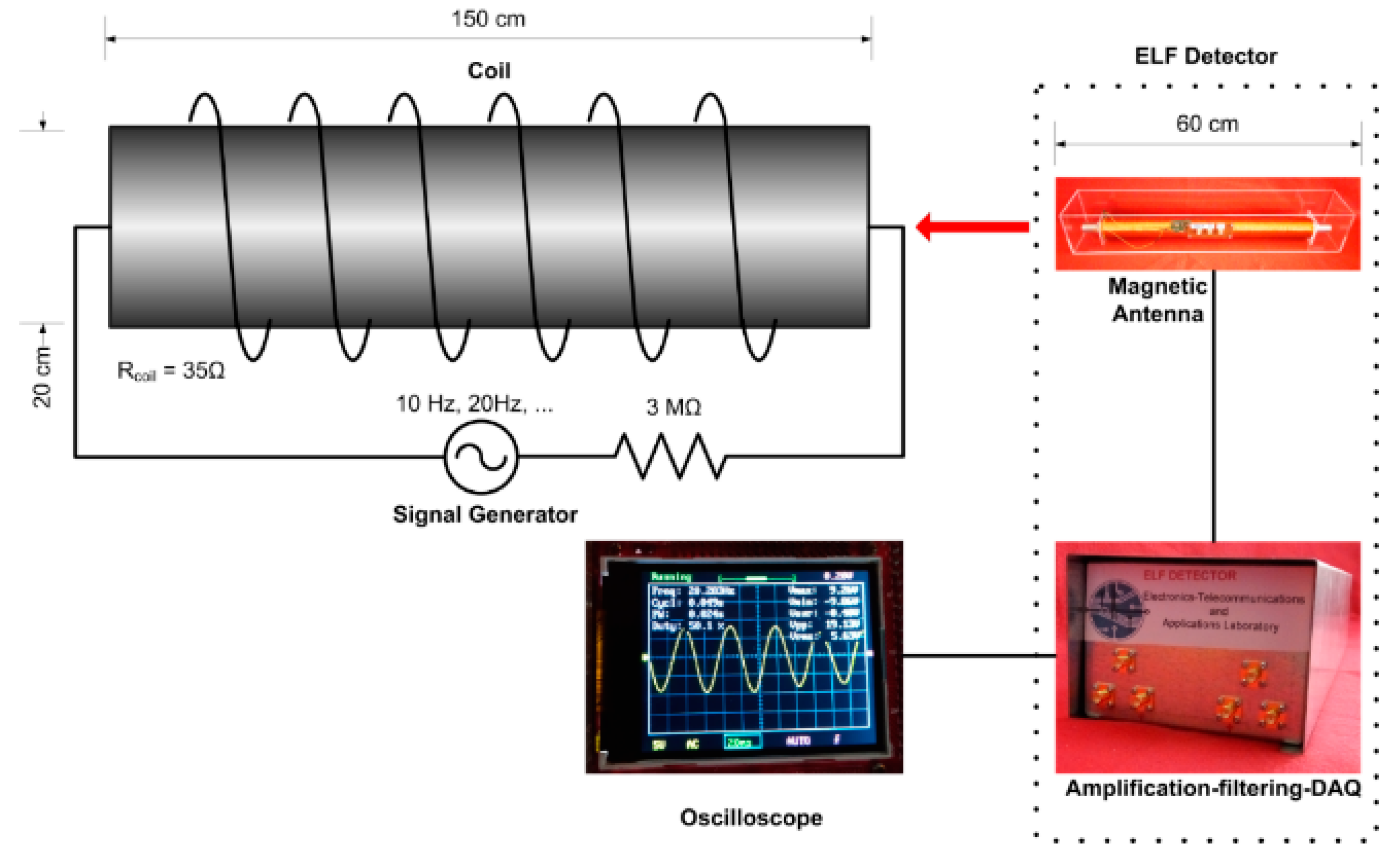
The entire test fixture is depicted in
Figure 1 and consists of the constructed coil, the signal generator, and the oscilloscope. The device to be calibrated is the magnetic antenna and its associated electronics (amplification-filtering data acquisition). The Electronics-Telecommunications and Applications (ETA) laboratory (Lab) ELF SR magnetic antenna detector was used as the device to be calibrated. It must be stressed that one of the most important requirements that have to be met in this procedure is to keep the external magnetic interferences (noises) as low as possible. Therefore, the whole test fixture presented in
Figure 1, as well as measurements, took place at the ELF detector installation site far away from an urban environment [
35]. The magnetic field generated inside the constructed coil is captured by the magnetic antenna exactly in the same way the SR waves are captured in the free air. The design of ETA Lab’s SR magnetic antenna receiver started at the end of 2012. In 2014, the first prototype was implemented, while from 2015 to 2016, preliminary measurements took place in the region of Epirus North West Greece [
36,
37]. After several updates and tuning ups, the SR system was installed near the Doliana village in the Ioannina prefecture, Northwestern Greece. The ETA Lab’s SR magnetic antenna receiver started measuring on the 19 January 2016 till now with concurrent recordings and measures up to six SR modes [
30,
38]. Recent discontinuities in the SR spectra of the detection station have shown a possible interconnection between lithospheric seismic activity and the atmospheric electromagnetic ELF background [
16,
17]. In June 2016, the measurement station was added to the list of worldwide SR stations. In February 2019, ETA Lab’s SR data were made available to the scientific community through the MIT SuperCloud for the multi-station inversion calculation for global lightning activity. ETA Lab’s ELF detector consists of the magnetic antenna and the signal conditioning chain [
30] as well as the data acquisition (DAQ) chain [
34].
2.1. Magnetic Antenna
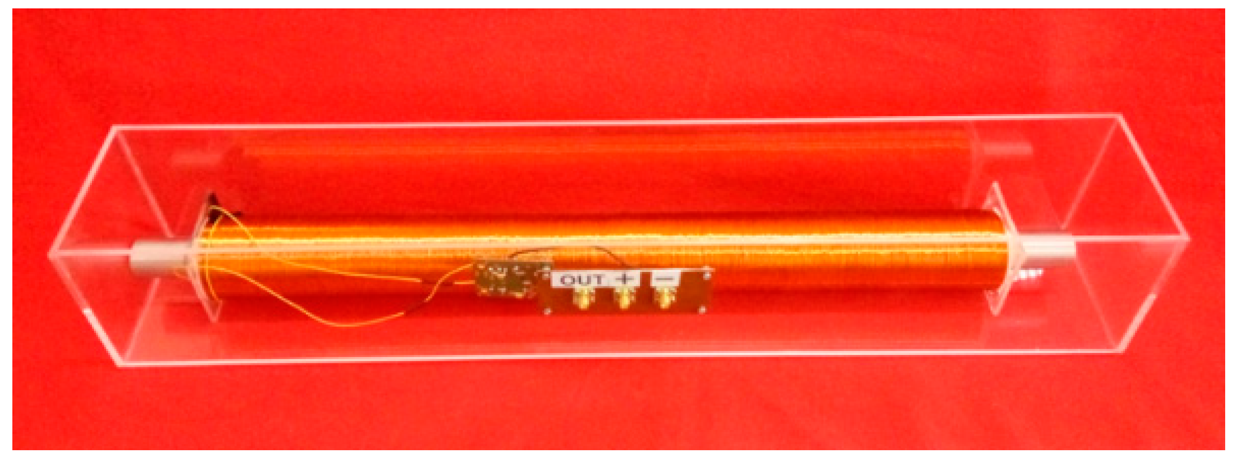
The magnetic induction antenna that was used, illustrated in
Figure 2, is 60 cm long. The cylindrical rod material of the detector is mu-metal with a diameter of 2.5 cm and consists of 90,000 turns of 0.25 mm copper wire around it. The inductance of the magnetic antenna is measured and has a value of 420 H. The self-resonant frequency of the magnetic antenna is measured to be 250 Hz. From the measured inductance and the resonant frequency, the parasitic capacitance of the magnetic antenna is found to be 965 pF. The practical operating frequency range of this antenna is below 45 Hz, near the sixth mode of the SR resonances, where the antenna has a linear response, and frequencies above 45 Hz are out of interest.
As it can be seen from Faraday’s law, depicted in Equation (2), the larger the relative magnetic permeability of the rod, the larger the induced voltage of the detected signal:
where
N is the number of turns of the induction coil,
μr is the relative magnetic permeability of the rod used, and Δ
Φ/Δ
t is the rate of change of magnetic flux. Therefore, it is almost imperative to use ferromagnetic rod materials that exhibit very high magnetic permeability, of a greater order than 10
5, thus providing a high induced voltage amplitude. Such a material with very high magnetic permeability is the mu-metal (ASTM A753 Alloy 4) that was used. Besides, it exhibits minimal coercive force, very low core loss, and remanence. However, since in the implemented antenna, the core used is an open-ended rod, the resultant apparent magnetic permeability is many times smaller than the mu-metal magnetic permeability itself. Taking into account the theoretical approach, the resultant apparent magnetic permeability of an open-ended rod depends not only on the magnetic permeability of the ferromagnetic material used but also on the induction coil geometry through demagnetization factor
ND. The above dependency is depicted by Equations (3) and (4):
where
m is the core length to diameter ratio
μe is the effective relative permeability, and
μr is the relative core permeability.
It is also clear that for
μr values of 10
5 order, Equation (3) is simplified to Equation (5) as:
In ETA Lab’s detector,
m = 24 (derived from 60/2.5),
ND = 0.004984724, and
μe = 200.6.
Although this theoretical value is a good approximation of the expected apparent magnetic permeability value of the rod, it might be different from the real, experimentally measured value.
2.2. Constructed Coil
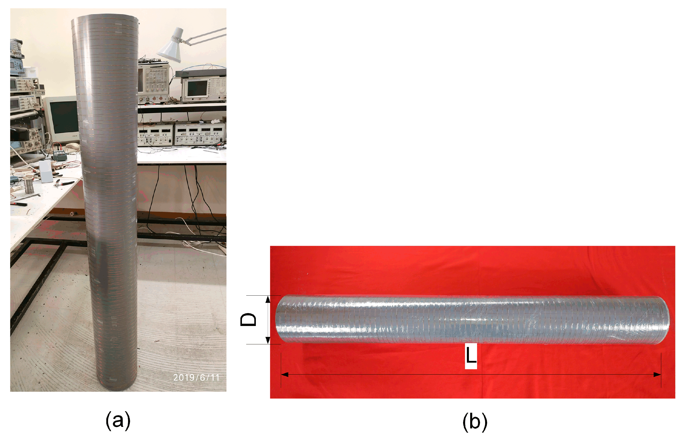
The proposed test fixture allows the precise measurement of the real (apparent) value of the rod’s magnetic permeability used in the detection antennae; thus, it is essential to know this value since, according to Equation (2), it defines the gain of the antenna. The implemented absolute and accurate calibration test fixture consists of a large enough test solenoid where the length
L is 150 cm, its diameter
D is 20 cm, and the number of equidistant turns
NS is 150 (one turn per centimeter). The solenoid with these dimensions, considered to produce a homogeneous magnetic field for the inner Schumann magnetic antenna detector dimensions [
39], as for an infinite length solenoid given by:
where
I is the current flow, and
μ0 is the vacuum permeability, considered to be 4π 10
−7 Hm
−1. The constructed coil is depicted in
Figure 3a,b. The magnetic field generated inside the coil is measured extensively and found to be homogenous better than 98% in the area of interest that is sufficient enough for the test fixture purposes.
2.3. Signal Generator
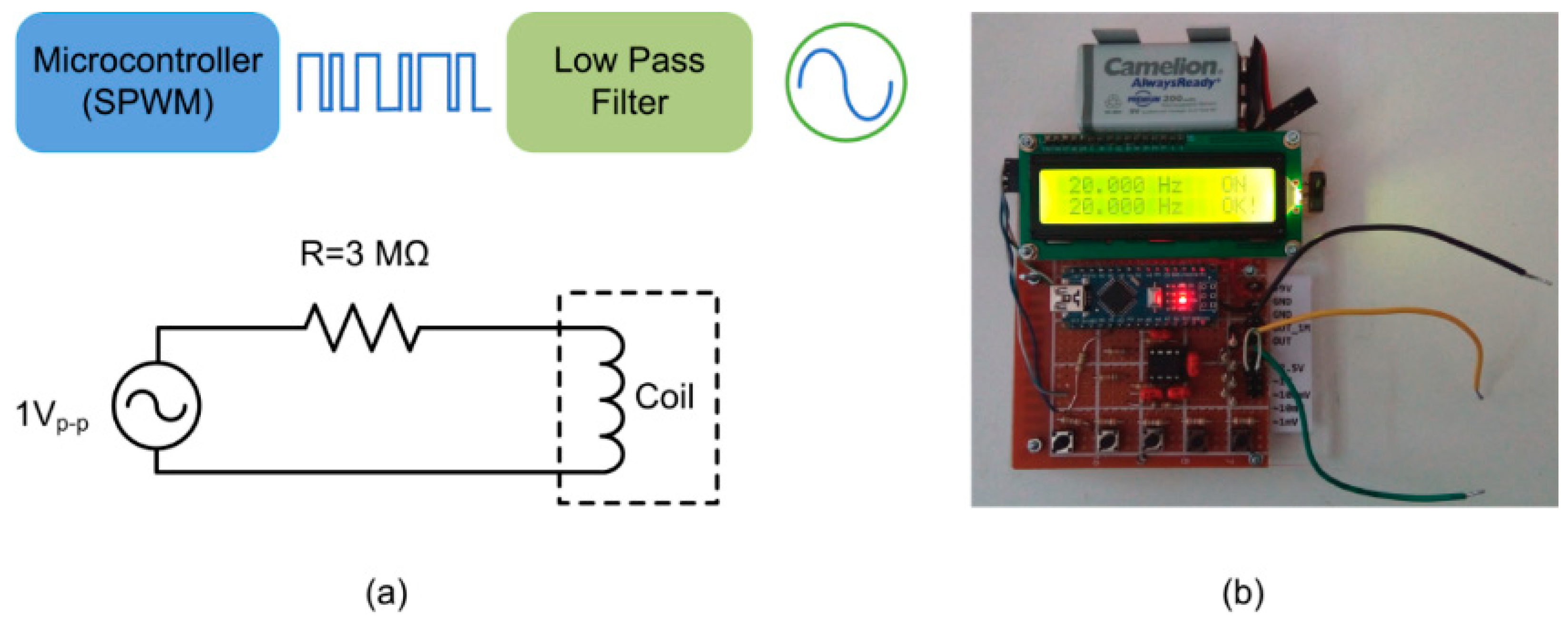
The final purpose of this apparatus is to generate magnetic fields of the order of pT. Therefore, extreme care must be taken in order to avoid any external noise and interference. To minimize as much as possible any external noise coming from the mains, a 9 V powered signal generator, as shown in
Figure 4b, was implemented. This generator provides digitally produced sinusoidal waveforms (SPWM). The frequency range is 1 Hz–1 kHz with a step of 1 Hz. The output has a fixed peak-to-peak value of 1 V, and the PWM frequency is 32 kHz. It must be pointed out that both frequency and amplitude are very accurate. The circuit uses the development board Arduino Nano that is based on the microcontroller ATmega328P by Microchip Technology Inc. The microcontroller is programmed to produce a time-variable PWM signal via a dedicated I/O line output.
The variable duty cycle corresponds to a sinus waveform (SPWM). This square-shaped signal is filtered with a fourth order Butterworth active low-pass filter using the Sallen–Key topology. The active low-pass filter uses the operational amplifier LM358 by Texas Instruments Inc. and has a unity gain, and the cut-off frequency is 212 Hz, eliminating the PWM base frequency and the harmonics allowing only the DC component to pass, thus producing the desired ELF sinusoidal signal. The filter is designed to have a passband large enough for the SR range of 0–50 Hz in order to keep the output amplitude constant in this range.
As can be seen from
Figure 4a, the solenoid is fed with 1 V through R, which is a 3 MΩ resistor. In this case, the current flowing through the solenoid is
Ιcoil = 0.333 μA. By substituting this value in Equation (6), the resultant magnetic flux density is 42 pT.
This magnetic flux density creates a signal that is detected and measured at the amplifier output.
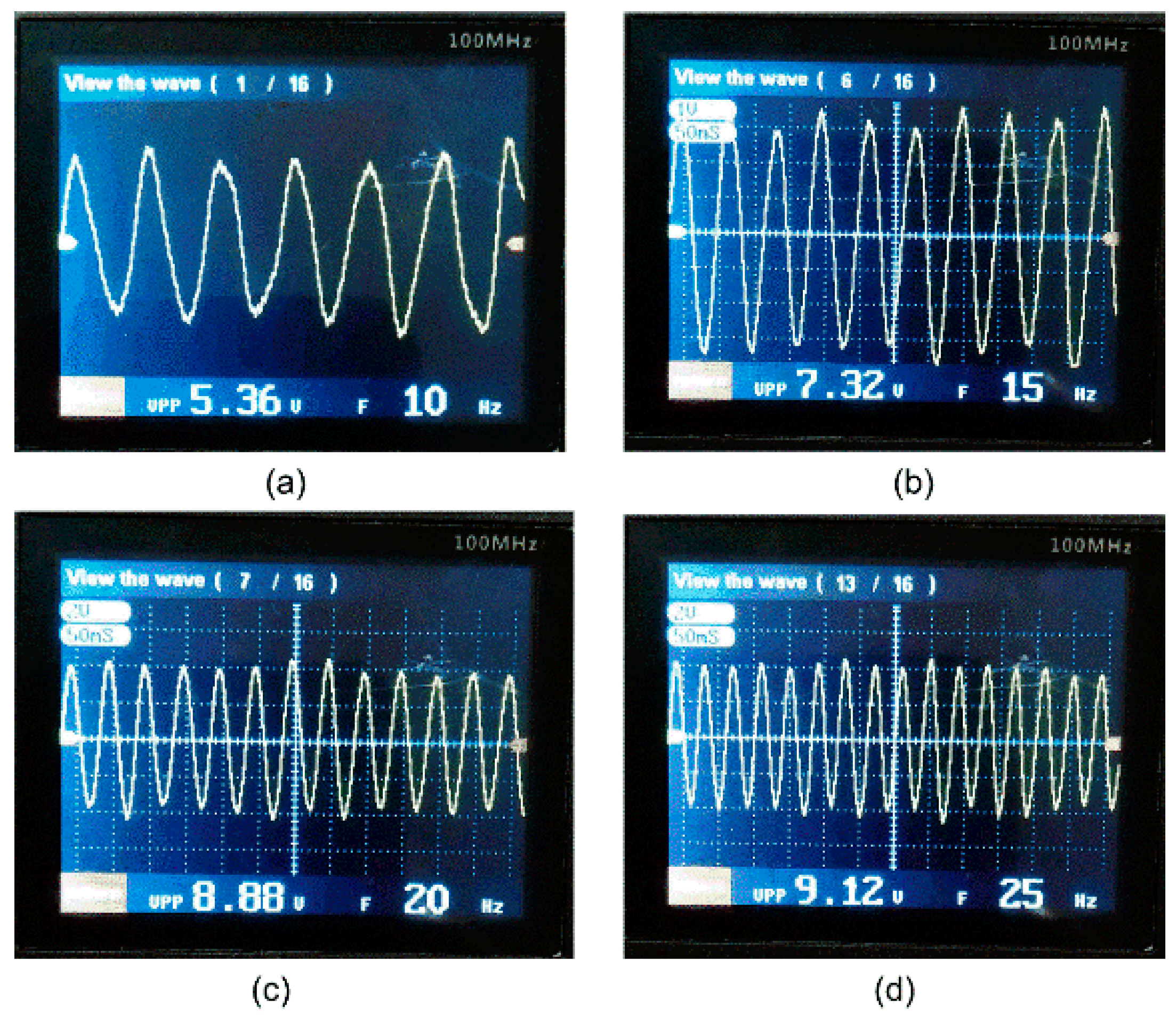
Figure 5 shows some acquired measurements that were taken at different frequencies, more specifically at 10, 15, 20, and 25 Hz. For each of these frequencies, the amplitude of the amplifier output was measured in order to calculate the system’s sensitivity, which is the output voltage (mV) for the detector input magnetic flux (pT). Since the outputted sinusoidal signal has additive noise, as is visible in
Figure 5, the amplitude of the signal was estimated by using nonlinear least square regression, fitting the experimental data in a sinusoidal model as expressed in Equation (7). For that purpose, the output signal was sampled by ETA Lab’s data logger [
34] at a rate of 2400 samples/sec, and the stored waveforms were processed in order to estimate the sine amplitude. The parameters
a,
φ, and
b are to be estimated, and we are interested in the sine amplitude
a as:
where
y stands for the sampled data vector,
t is the time vector,
a is the sine amplitude,
ω is the angular frequency,
φ is the phase offset, and
b is the total voltage offset of the signal. The frequency, and therefore the angular frequency, is known and as mentioned above has four values (10, 15, 20, and 25 Hz).
2.4. Amplification-Filtering (Data Acquisition)-DAQ
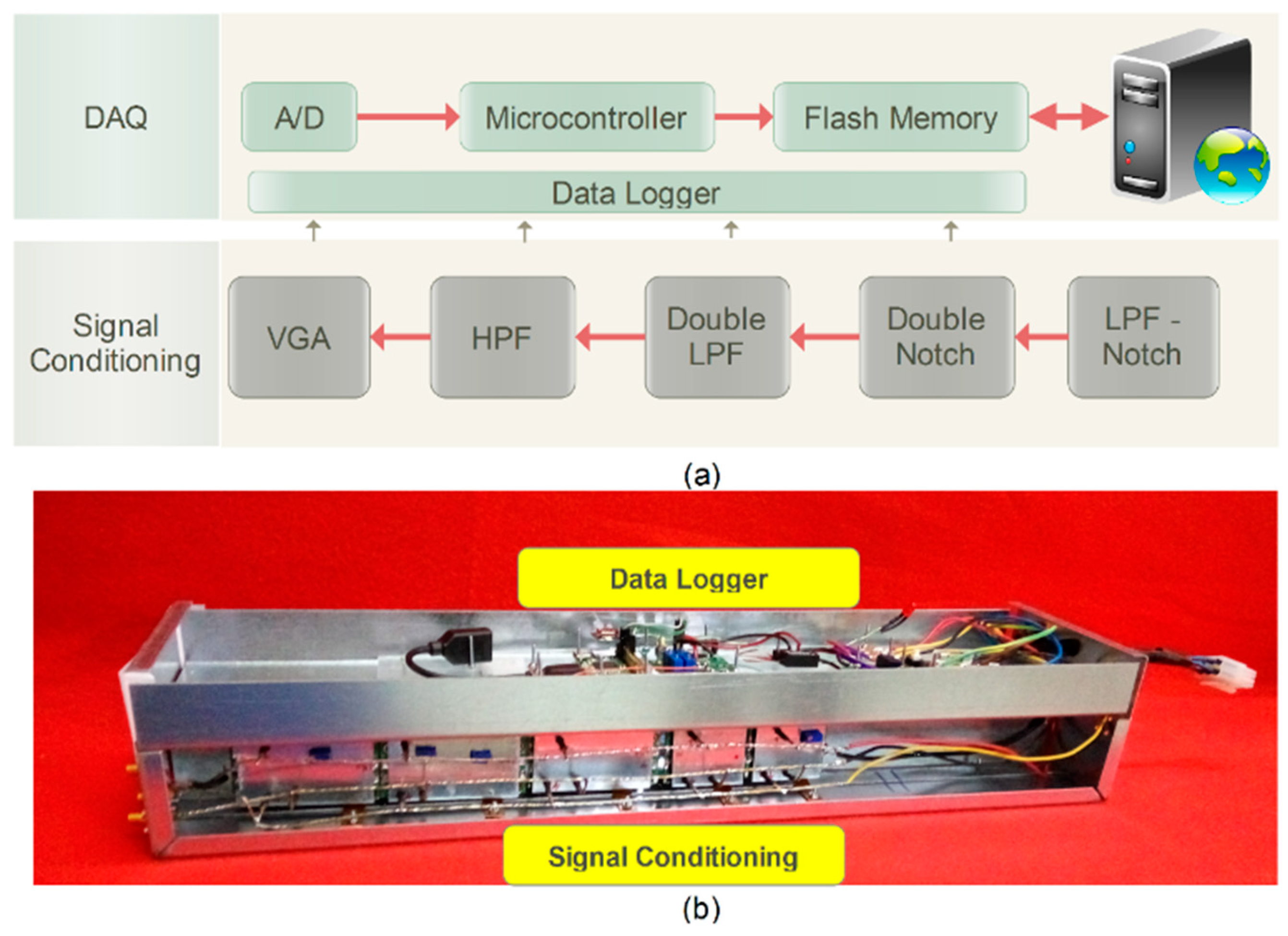
The Electronics-Telecommunications and Applications (ETA) laboratory (Lab) ELF SR magnetic antenna detector was used as the device to be calibrated. The ELF receiver is a customized lab-made device that consists of the magnetic antenna, the amplifying filtering (signal conditioning), and data acquisition (DAQ) chains. A block diagram of signal conditioning and DAQ is depicted in
Figure 6a, while the magnetic antenna [
30,
34] is depicted in
Figure 2. The signal conditioning stage receives the ELF signal captured from the magnetic antenna. As shown in the block diagram of
Figure 6a, signal conditioning consists of filters and a voltage gain amplifier (VGA). The first filter stage consists of a second-order Sallen–Key low-pass filter and a 50 Hz Twin-T notch filter (LPF-Notch). The second stage consists of two cascaded 50 Hz Twin-T notch filters (Double Notch). The third stage of the filtering chain is based on two second-order low-pass filters in cascading connection (Double LPF). The fourth stage of the filtering chain involves a Sallen–Key high-pass filter topology (HPF) and, finally, the VGA adjusts the gain up to 20. The DAQ stage is based on low-power scalable ETA’s Lab prototype logger and consists of an A/D converter and a microcontroller. The logger’s sampling rate is programmable from 512 Hz to 19,200 Hz while the bit resolution is 18 bits. The sampling rate is set to 19,200 Hz and the logger averages the samples by a factor of 8, thus outputting a sampling rate of 2400 Hz. After averaging, the 16 most significant bits are used. Raw data are stored in an SD card. Further signal processing is performed offline through a PC. SR data and spectra are available to the scientific community through the internet. The constructed ELF detector is shown in
Figure 6b. On top of the amplifying and filtering chain is located in the data acquisition chain. Below is located the amplification and filtering chain that comprises two channels for simultaneous detection of North–South and East–West Schumann resonances. The amplification and filtering chain comprises five units electromagnetically shielded, as can be seen in
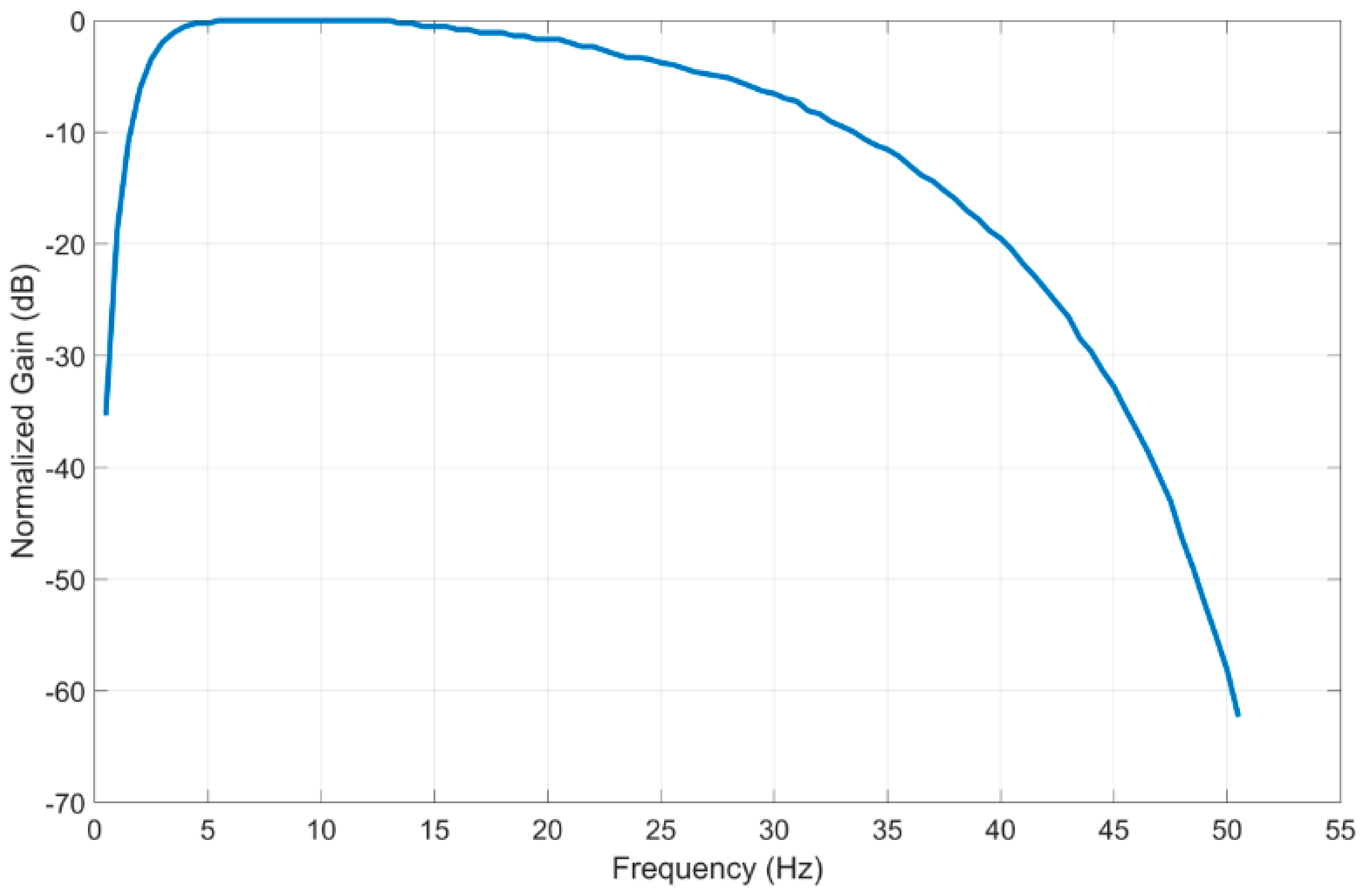
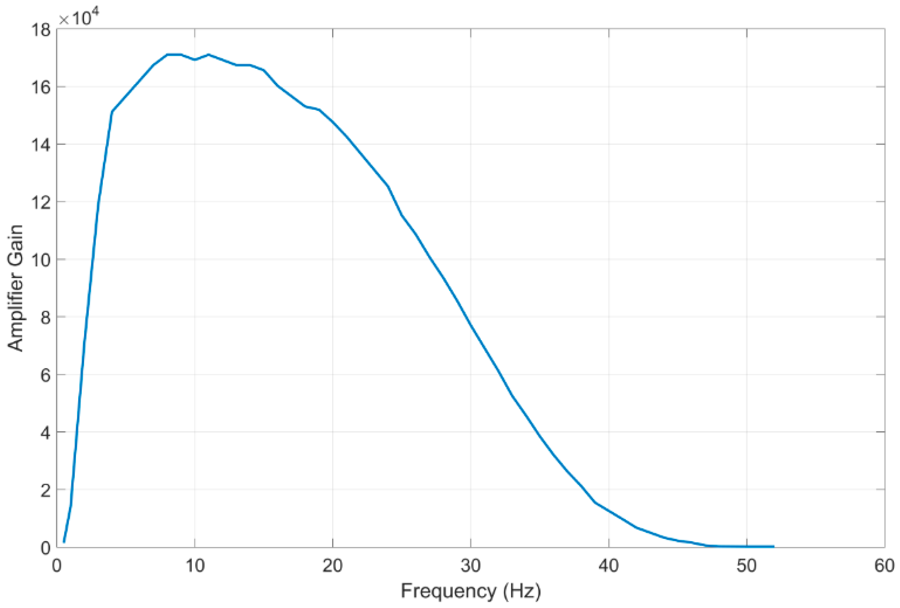
Figure 6b. Moreover, all stages are mounted inside a metallic box thus assuring additional shielding of each chain. An identical amplification and filtering chain is located at the bottom left side of the isolated metallic case. The maximum amplification gain is 171,000, and the attenuation of any 50 Hz noise (induced by the mains in the detection coil) equals 60 dB. The total frequency response of the amplifier–filtering unit is shown in
Figure 7. A detailed analysis of the ELF magnetic antenna detector, including amplification and filtering schemes, magnetic antenna, and data acquisition process, can be found in the literature [
30,
34,
36,
37,
38].
3. Measurement Results
Table 1 shows the measurement results, using the sinusoidal fitting method as described above. These are the responses of the system for input of 42 pT, as mentioned before, on our magnetic coil for different frequencies. For example, at 20 Hz, the sensitivity of the magnetic antenna can be calculated as 58.94 μV/42 pT = 1.4 μV/pT, and the total system sensitivity is 8.70 V/42 pT = 207 mV/pT.
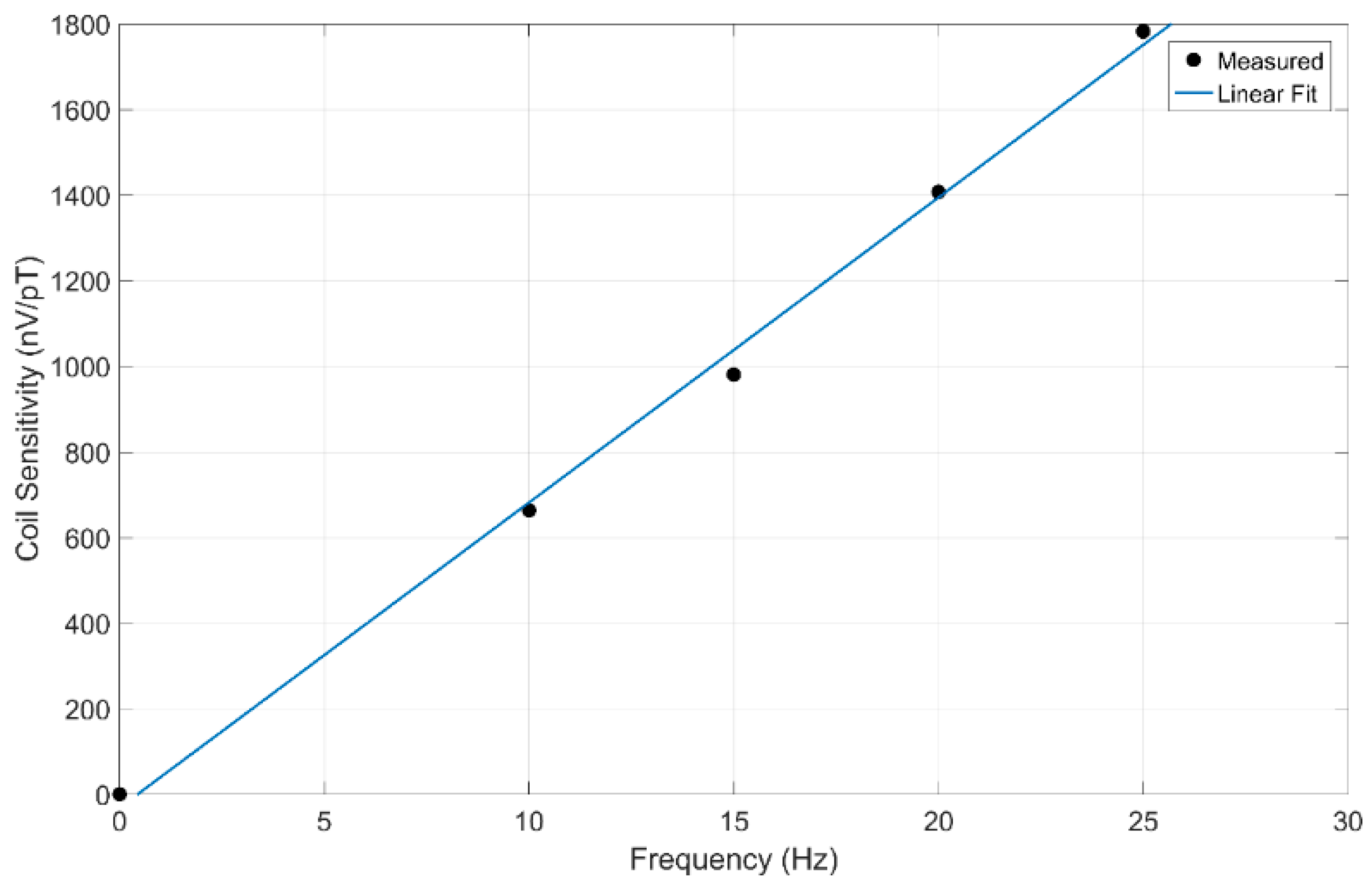
Figure 8 depicts the four measured sensitivity values of the magnetic receiver coil versus frequency. Since a magnetic coil is expected theoretically to have an output voltage amplitude linearly proportional to the frequency (Equation (2)), the best linear fit was estimated as one may observe in this Figure, and the final estimated sensitivity of the coil is found through the line slope equal to 70 nV/pT/Hz.
Figure 9 depicts the measured signal conditioning circuit (amplification and filtering) gain against frequency. The corresponding values at the selected frequencies are visible in the third column of
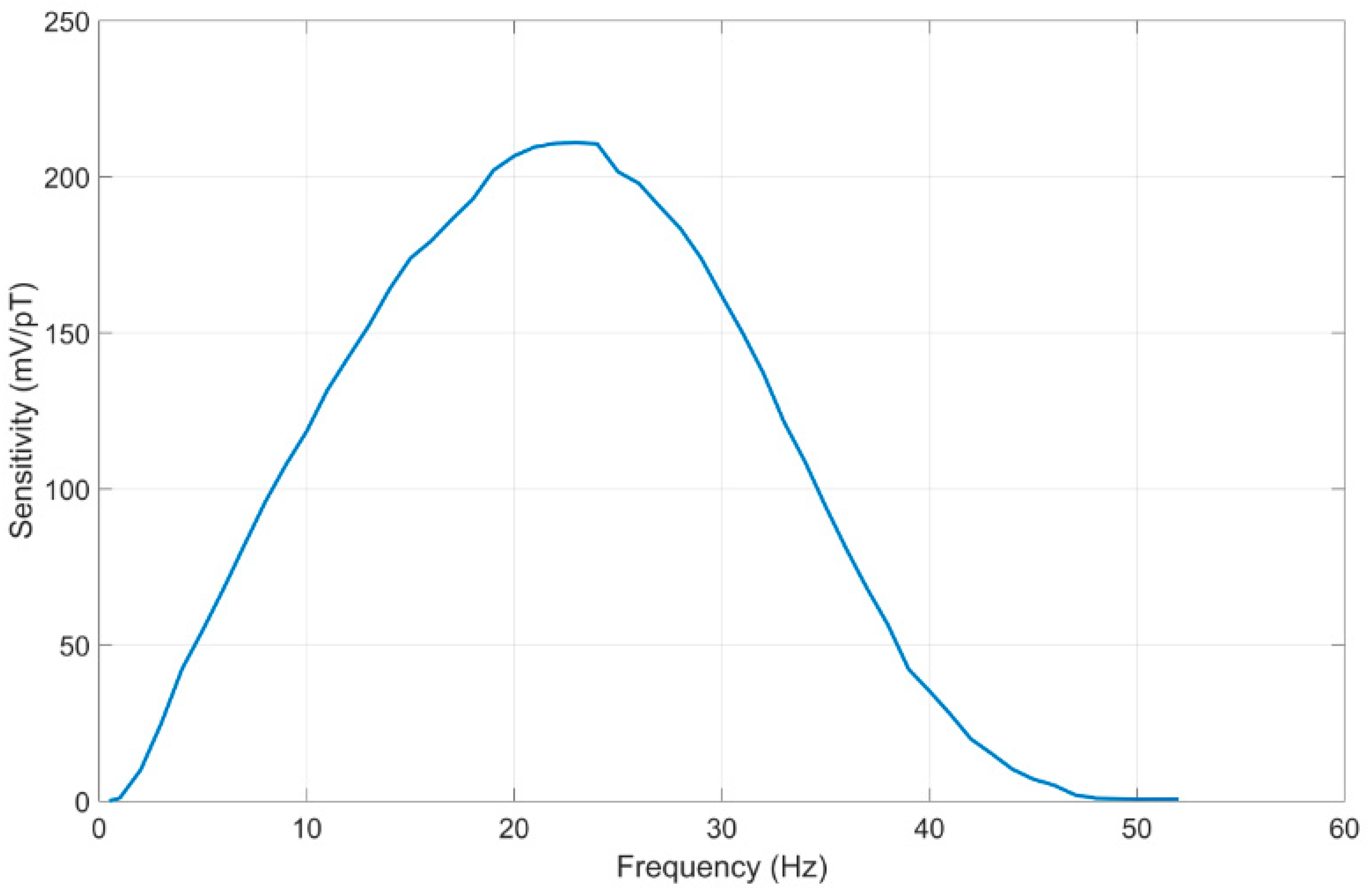
Table 1. The total system (antenna and signal conditioning) as a function of the frequency is shown in
Figure 10.
The proposed experimental setup allows the estimation of the apparent permeability of the mu-metal core used. A magnetic flux sinusoidal waveform was considered such as the one produced in the experimental procedure with the generator. The mathematical expression is shown in Equation (8):
where
A is the cross-section area of the core calculated as
,
B0 is the magnetic flux density amplitude, and f is the frequency. We assume the total magnetic flux inside the coil to be approximately equal to the flux inside the core expecting that the core has a relatively large effective permeability. Following Faraday’s law in Equation (2), the rate of change of the magnetic flux is given by:
The induced voltage is also a sinusoidal waveform and by substitution of previous in Equation (2), the induced voltage amplitude value is:
where
μe is the core apparent permeability and, for simplicity, a frequency of 1 Hz and a magnetic flux density amplitude of 1 pT were considered. Taking into account that the final estimated sensitivity is 70 nV/pT/Hz, the core magnetic permeability exported by Equation (10) is
μe = 70/0.2773 ~
μe = 252. This is an estimation according to our measurements, and as mentioned above, we find a value greater than the theoretical one, which is about 200. The total equivalent input voltage noise of the detector is 55 nV as measured and presented in [
30], resulting mainly from the thermal noise of the coil, which is about 50 nV, and also the amplifier input noise found experimentally to be about 20 nV, considering the bandwidth of our interest, 0–50 Hz.
In the present work, we have estimated the sensitivity of the magnetic antenna and total detector as it is depicted in
Figure 8 and
Figure 10. Taking into account that the system has a maximum sensitivity around the area of 20 Hz, where the antenna has a sensitivity of about 1400 nV/pT, we roughly may calculate an estimate of the input equivalent noise to ETA Lab’s detector as (55 nV)/(1400 nV/pT) = 0.04 pT, that is the equivalent magnetic flux density noise at the input of the ELF detector.
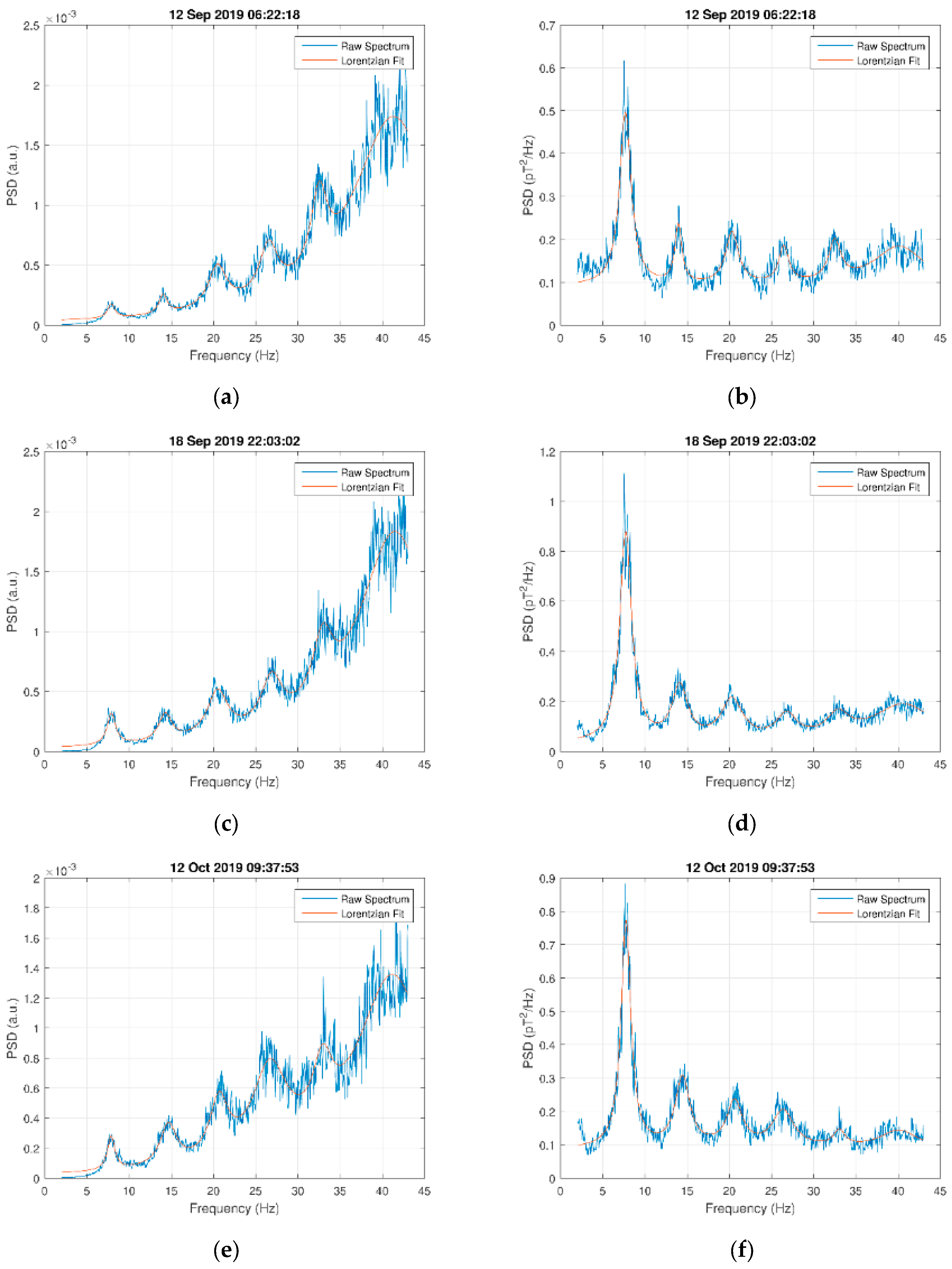
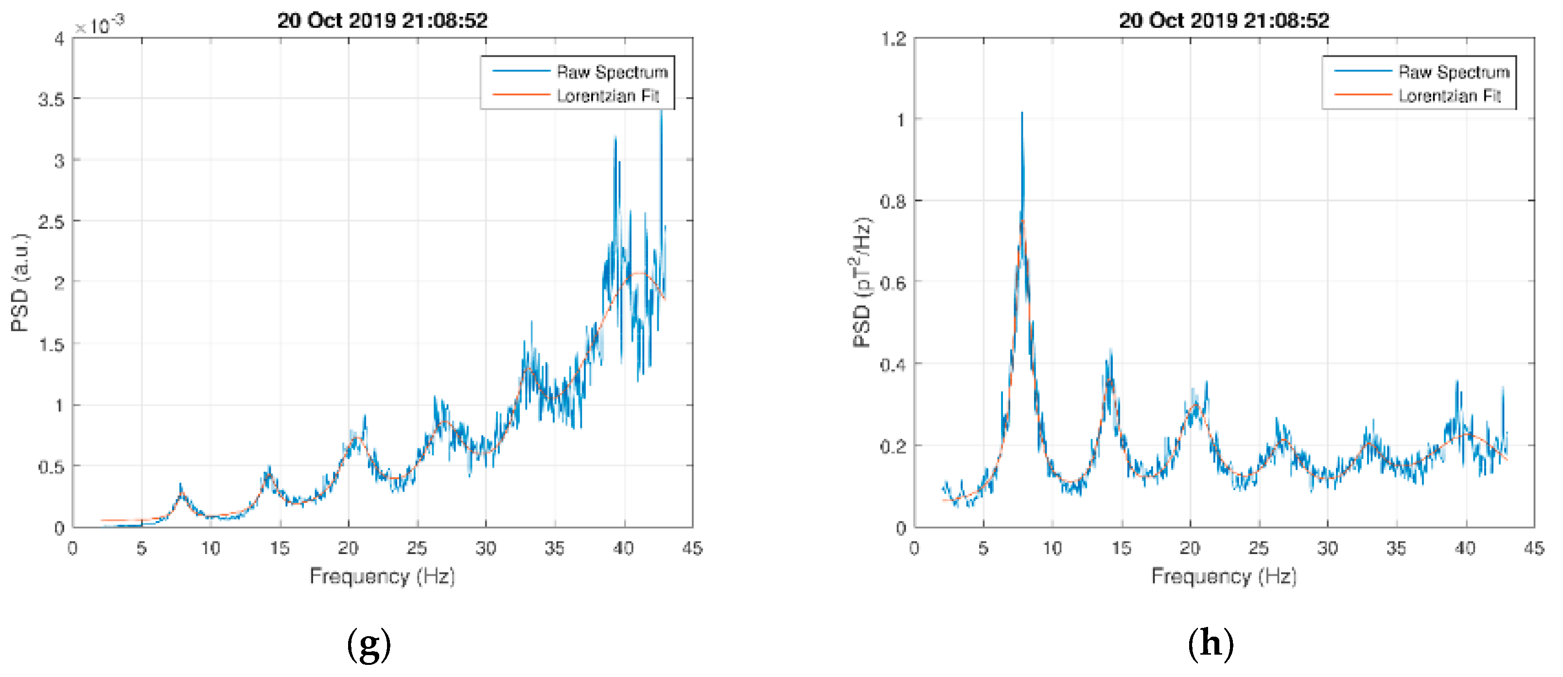
In
Figure 11, recent measurements taken from ETA Lab’s system are shown in the fall of 2019. A nonlinear least square regression, using a Lorentzian-like function for the mathematical model for the resonance estimation, is performed on the raw spectrum. On the left images, the spectra are calculated by inverting the effect of the amplification and filtering system but not the magnetic coil. On the right, we observe the final spectrum in the input of the receiver (magnetic coil) inverting the effect of the antenna as well. Therefore, the vertical axis is displayed in corresponding units of the magnetic field’s spectral power density. The peak frequencies were
fn = [7.8, 14.7, 20.2, 26.5, 33, 40] Hz, while the power spectral density (PSD) values for the six modes are clearly shown and varying from 0.2 to 0.9 pT
2/Hz, which yields a signal-to-noise ratio greater than 10.
4. Conclusions
The Schumann resonances (SR) appear as peaks with extremely low amplitudes of a few pT at frequencies ranging from 7 Hz and reaching up to 40 Hz. There is a vast amount of literature on Schumann resonances’ correlation with several physical phenomena. However, only a few studies have focused on the electronics of the receiver platform, which remains vital to have reliable measurements and accurate SR spectra. It is a fact that there are a limited amount of data and SR spectra in public scientific sources on the subject. The available SR spectra are mostly presented in arbitrary units (such as dB). Furthermore, most spectra appear as mean values in 10 min and 30 min time windows, and there are not instant for the SR spectra. In order to export accurate SR spectra, an ELF Schumann receiver must be precisely calibrated. To our best knowledge, no previous study has presented a test fixture for the calibration of an ELF Schumann resonance magnetic antenna receiver. The proposed test fixture allows the scientific community to adopt a straightforward methodology for the calibration of ELF SR magnetic antenna receivers. In this way, SR data and spectra could be exported in absolute units rather than arbitrary units. Thus, the ability to correlate data across the world will facilitate understanding of a variety of global geophysical phenomena related to SR resonances. The detector is based on a magnetic coil that serves as an ELF antenna and signal conditioning DAQ chain. This calibrating platform allows the precise measurement of the sensitivity of our system, the measurement of the apparent permeability of the core of the magnetic coil antenna, and the equivalent input noise of ETA Lab’s detector. The sensitivity of the magnetic antenna is 70 nV/pT/Hz considering a sinusoidal input signal. The total sensitivity of the system, including the amplifier and filters, is frequency-dependent and exhibits a maximum sensitivity of 210 mV/pT around 20 Hz. The total input noise to the ELF detector is measured to be approximately as low as 0.04 pT. Finally, the experimental procedure results that the apparent magnetic permeability of the mu-metal rod of the magnetic antenna coil has a value of 250.

 ,
, 


