A Novel Image-Restoration Method Based on High-Order Total Variation Regularization Term

Abstract

This paper presents two new models for solving image the deblurring problem in the presence of impulse noise. One involves a high-order total variation (TV) regularizer term in the corrected total variation L1 (CTVL1) model and is named high-order corrected TVL1 (HOCTVL1). This new model can not only suppress the defects of the staircase effect, but also improve the quality of image restoration. In most cases, the regularization parameter in the model is a fixed value, which may influence processing results. Aiming at this problem, the spatially adapted regularization parameter selection scheme is involved in HOCTVL1 model, and spatially adapted HOCTVL1 (SAHOCTVL1) model is proposed. When dealing with corrupted images, the regularization parameter in SAHOCTVL1 model can be updated automatically. Many numerical experiments are conducted in this paper and the results show that the two models can significantly improve the effects both in visual quality and signal-to-noise ratio (SNR) at the expense of a small increase in computational time. Compared to HOCTVL1 model, SAHOCTVL1 model can restore more texture details, though it may take more time.

1. Introduction

In the field of electronics and information, signal processing is a hot research topic, and as a special signal, the study of image has attracted the attention of scholars all over the world [1,2,3]. In image processing, image restoration is one of the most important issues and this issue has received extensive attention in the past few decades [4,5,6,7,8,9,10,11]. Image restoration is a technology that uses degraded images and some prior information to restore and reconstruct clear images, to improve image quality. At present, this technology has been widely used in many fields, such as medical imaging [12,13], astronomical imaging [14,15], remote sensing image [16,17], and so on. In this paper, the problem of image deblurring under impulse noise is considered. Normally, camera shake, and relative motion between the target and the imaging device may cause image blurring; while in digital storage and image transmission, impulse noise may be generated.

In the process of image deblurring under impulse noise, the main task is to find the unknown true image $\mathit{x}\in R^{n^2}$ from the observed image $\mathit{f}\in R^{n^2}$ defined by

$$\mathit{f}=N_{imp}(\mathit{K}\mathit{x})$$

(1)

where $N_{imp}$ denote the process of image degradation by impulse noise, and $\mathit{K}\in R^{n^2\times n^2}$ is a blurring operator. It is known that when $\mathit{K}$ is unknown, the model deals with blind restoration, and when $\mathit{K}$ is known, it deals with image denoising.

There are two main types of impulse noise: salt-and-pepper noise and random-valued noise. Suppose the dynamic range of $\mathit{x}$ to be $[d_{min},d_{max}]$, for all $(i,j)\in \Omega =\left\{1,2,\dots ,n\right\}\times \left\{1,2,\dots ,n\right\}$, the $x_{i,j}$ is the gray value of an image $\mathit{x}$ at location $(i,j)$, and $d_{min}\le f_{i,j}\le d_{max}$. For 8-bit images, $d_{min}=0$ and $d_{max}=255$. Then for salt-and-pepper noise, the noisy version $\mathit{f}$ at pixel location $(i,j)$ is defined as

$$f_{i,j}=\left\{\begin{array}{cc}{d}_{min},\hfill & \mathrm{with}\mathrm{probability}\frac{s}{2},\hfill \\ d_{max},\hfill & \mathrm{with}\mathrm{probability}\frac{s}{2},\hfill \\ x_{i,j},\hfill & \mathrm{with}\mathrm{probability}1-s,\hfill \end{array}\right.$$

(2)

where s is the noise level of the salt-and-pepper noise.

For random-valued noise, the noisy version $\mathit{f}$ at pixel location $(i,j)$ is defined as

$$f_{i,j}=\left\{\begin{array}{cc}{d}_{i,j},\hfill & \mathrm{with}\mathrm{probability}r,\hfill \\ x_{i,j},\hfill & \mathrm{with}\mathrm{probability}1-r,\hfill \end{array}\right.$$

(3)

where $d_{i,j}$ is uniformly distributed in $d_{min}\le f_{i,j}\le d_{max}$ and r is the noise level of random-valued noise. It is clear that compared with salt-and-pepper noise, the random-valued noise is more difficult to remove since it can be arbitrary number in $d_{min}\le f_{i,j}\le d_{max}$.

For image-restoration problem contaminated by impulse noise, the widely used model is composed of data fidelity term measured by ${\ell }_1$ norm and the TV regularization term, which is called TVL1 model [18,19,20]. TVL1 model can effectively preserve image boundary information and eliminate the influence of outliers, so it is especially effective to deal with non-Gaussian additive noise such as impulse noise. Now, it has been widely and successfully applied in medical image and computer vision.

However, TVL1 model has its own shortcomings, which makes it ineffective in dealing with high-level noise, such as 90% salt-and-pepper noise and 70% random-valued noise [21]. In recent years, a large number of scholars have devoted themselves to this research, and a lot of algorithms have been proposed [22,23,24,25,26,27]. In 2009, Cai et al. [22] proposed a two-phase method, and in the first phase, damaged pixels of the contaminated image were explored, then in the second phase, undamaged pixels were used to restore images. Numerical experiments show that the two-phase method is superior to TVL1 model, it can handle as high as 90% salt-and-pepper noise, and as high as 55% random-valued noise, while it cannot perform effectively when the level of random-valued noise is higher than 55%. Similarly, considering the problem that TVL1 model may deviate from the data-acquisition model and the prior model, especially for high levels of noise, Bai et al. [23] introduced an adaptive correction procedure in TVL1 model and proposed a new model called the corrected TVL1 (CTVL1) model. The main idea is to improve the sparsity of the TVL1 model by introducing an adaptive correction procedure. The CTVL1 method also uses two steps to restore the corrupted image, the first step generates an initial estimator by solving the TVL1 model, and the second step generates a higher accuracy recovery from the initial estimator which is generated by TVL1 model. Meanwhile, for higher salt-and-pepper noise and higher random-valued noise, by repeating the correction step for several times, high levels of noise can be removed very well. Numerical experiments show that the CTVL1 model can remove salt-and-pepper noise as high as 90%, and remove random-valued noise as high as 70%, which is superior to the two-phase method.

Similar to CTVL1 method, Gu et al. [24] combined TV regularization with smoothly clipped absolute deviation (SCAD) penalty for data fitting, and proposed TVSCAD model; Gong et al. [25] used minimax concave penalty (MCP) in combination with TV regularization for data fitting, and he proposed TV-MCP model. Numerical experiments show that both TVSCAD model and TV-MCP model can achieve better effects than two-phase method. But compared with CTVL1 method, their contributions mainly focus on the convergence rate, and they did not improve much in terms of impulse noise removal.

However, as is described in [28], TV norm may transform the smooth area to piecewise constants, the so-called staircase effect. To overcome this deficiency, the efficient way is to replace the TV norm by a high-order TV norm [29]. In particular, second-order TV regularization schemes are widely studied for overcoming the staircase effects while preserving the edges well in the restored image. In [30], Si Wang proposed a combined total variation and high-order total variation model to restore blurred images corrupted by impulse noise or mixed Gaussian plus impulse noise. In [27], based on Chen and Cheng’s an effective TV-based Poissonian image deblurring model, Jun Liu introduced an extra high-order total variation (HTV) regularization term to this model, which can effectively remove Poisson noise, and its effect is better than Chen and Cheng’s model. In [31], Gang Liu combined the TV regularizer and the high-order TV regularizer term, and proposed HTVL1 model, which can better remove the impulse noise contrast to TVL1 model. However, since TVL1 model has its own defects, the restoration of HTVL1 model is limited. Besides, the author did not consider the removal effect of random-valued noise.

In this paper, we continue to study the problem of image deblurring under impulse noise. The main contributions of this paper include: (1) Combining high-order TV regularizer term with CTVL1 model, a new model named high-order corrected TVL1(HOCTVL1) model is proposed and the alternating direction method of multipliers (ADMM) is used to solve this new model. Compared with existing models, our model can get higher signal-to-noise (SNR) in dealing with image deblurring under impulse noise. (2) The spatially adapted regularization parameter is introduced into the HOCTVL1 model and SAHOCTVL1 model is proposed. Compared to HOCTVL1 model, SAHOCTVL1 model can further improve the effects of image restoration in some degree.

The rest of this paper is organized as follows. In Section 2, a brief review of related work is made. In Section 3, the presentation of HOCTVL1 model is discussed, and  the HOCTVL1 algorithm is concluded. Section 4 introduces the spatially adapted regularization parameter selection scheme, and SAHOCTVL1 model is proposed. Numerical experiments are carried out in Section 5 and finally, the conclusion is presented in Section 6.

2. Brief Review of Related Work

For recovering the image corrupted by blur and impulse noise, the classic method is TVL1 model. Since a lot of literature [19,20,31,32,33] demonstrates that using L1-fidelity term for image restoration under impulse noise can achieve good effects, the TVL1 model is expressed as

$$\underset{x}{min}TV(\mathit{x})+\lambda {∥\mathit{K}\mathit{x}-\mathit{f}∥}_1$$

(4)

where $\mathit{f}$ is the observed image, $\mathit{x}$ denotes the restoration image, $\mathit{K}$ is a blur matrix, $\lambda$ is a regularization parameter which is greater than zero, $TV(\mathit{x})$ represents the discrete TV norm and is defined as $TV(\mathit{x})={\displaystyle \sum _{1\le i,j\le n}}∥{(\mathit{D}\mathit{x})}_{i,j}∥$. Here, $\mathit{D}$ denotes the discrete gradient operator (under periodic boundary conditions). The norm in $∥{(\mathit{D}\mathit{x})}_{i,j}∥$ can be taken as ${\ell }_1$ norm or ${\ell }_2$ norm. When the ${\ell }_2$ norm is used, the resulting TV term is isotropic and when the ${\ell }_1$ norm is used, the result is anisotropic. For more details about the TV norm, readers can refer to [18].

Since one of the unique characteristics of impulse noise is that an image corrupted with impulse noise still has intact pixels, the impulse noise can be modeled as sparse components, whereas the underlying intact image retains the original image characteristics [34]. Therefore, TVL1 model can efficiently remove abnormal value noise signals, and some points of the solution of the TVL1 model are close to the points of the original image. However, Nikolova [21] pointed out from the viewpoint of MAP that the solutions of the TVL1 model substantially deviate from both the data-acquisition model and the prior model, and Minru Bai [23] further pointed out that the TVL1 model does not perform well at the sparsity of $\mathit{K}\mathit{x}-\mathit{f}$ and there are many biased estimates produced by the TVL1 model. To overcome this shortcoming, Bai et al. took a correction step to generate an estimator to obtain a better recovery performance.

Given a reasonable initial estimator $\tilde{\mathit{x}}\in R^{n^2}$ generated by TVL1 model, let $\tilde{\mathit{z}}=\mathit{K}\tilde{\mathit{x}}-\mathit{f}$, then she established a model called CTVL1 model, which is defined as

$$\begin{array}{c}\underset{x,z}{min}\sum _{1\le i,j\le n}∥{(\mathit{D}\mathit{x})}_{i,j}∥+\lambda ({∥\mathit{z}∥}_1-⟨\mathit{F}(\tilde{\mathit{z}}),\mathit{z}⟩)s.t.\mathit{z}=\mathit{K}\mathit{x}-\mathit{f}\hfill \end{array}$$

(5)

Compared with TVL1 model, CTVL1 model is added a correction term $-⟨\mathit{F}(\tilde{\mathit{z}}),\mathit{z}⟩$, and $\mathit{F}$:$R^{n^2}\to R^{n^2}$ is an operator defined as

$$\mathit{F}(\mathit{z})=\left\{\begin{array}{c}\varphi (\frac{\mathit{z}}{{∥\mathit{z}∥}_{\infty }}),\mathit{z}\in R^{n^2}\setminus \left\{0\right\},\hfill \\ 0,\mathit{z}=0,\hfill \end{array}\right.$$

(6)

and the scalar function $\varphi$:$R\to R$ takes the form

$$\varphi (t)=\mathrm{sgn}(t)(1+{\epsilon }^{\tau })\frac{{\left|t\right|}^{\tau }}{{\left|t\right|}^{\tau }+{\epsilon }^{\tau }},\forall \mathrm{t}\in \mathrm{R},$$

(7)

where $\tau >0$ and $\epsilon >0$. Numerical results show that the CTVL1 model improves the sparsity of the data fidelity term $\mathit{K}\mathit{x}-\mathit{f}$ greatly for the images deblurring under impulse noise, to achieve a good denoising effect.

Since TV regularization term may come into staircase effects, in the past few years, a lot of researchers have devoted to solving this problem, and they concluded that replacing the TV norm by a high-order TV norm can get a better effect. The majority of the high-order norms involve second-order differential operators because piecewise-vanishing second-order derivatives lead to piecewise-linear solutions that better fit smooth intensity changes [35]. The second-order TV norm is defined as

$${({\mathit{D}}^2\mathit{x})}_{i,j}=({(\mathit{D}\mathit{x})}_{i,j}^{x,x},{(\mathit{D}\mathit{x})}_{i,j}^{x,y},{(\mathit{D}\mathit{x})}_{i,j}^{y,x},{(\mathit{D}\mathit{x})}_{i,j}^{y,y})$$

(8)

where ${(\mathit{D}\mathit{x})}_{i,j}^{x,x},{(\mathit{D}\mathit{x})}_{i,j}^{x,y},{(\mathit{D}\mathit{x})}_{i,j}^{y,x},{(\mathit{D}\mathit{x})}_{i,j}^{y,y}$ denote the second-order difference of the $\left(\left(j-1\right)n+i\right)$th entry of the vector $\mathit{x}$. Here we just briefly mention the concept of second-order TV norm, for more details, readers can refer to [36].

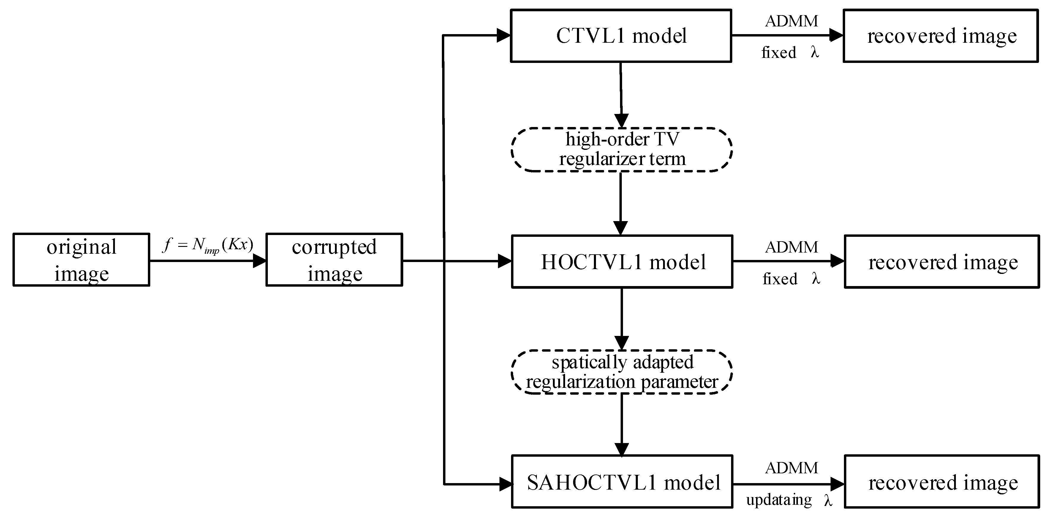
Figure 1 shows the diagram of image restoration. In this paper, two models named HOCTVL1 model and SAHOCTVL1 model are proposed and are used to recover the corrupted images.

Figure 1. The block diagram of solving image deblurring problem under impulse noise.

3. New Method: The HOCTVL1 Algorithm

In this section, the HOCTVL1 model is proposed and the selection of $\mathit{F}(\mathit{z})$ is talked about among CTVL1, SCAD and MCP models. Then ADMM is used to solve the proposed model and the HOCTVL1 algorithm is concluded.

3.1. Proposed New Model

Since the TV regularization norm $∥{(\mathit{D}\mathit{x})}_{i,j}∥$ can be taken as ${\ell }_1$ norm or ${\ell }_2$ norm, which is isotropic or anisotropic respectively. In [23,24,25,31], the authors all only consider the isotropic case, so in this paper, we will also only treat the isotropic case in detail, and the anisotropic case is similar to deal with. Based on this premise, the proposed high-order corrected TVL1 (HOCTVL1) model can be expressed as

$$\begin{array}{c}\underset{x,z}{min}{\displaystyle \sum _{1\le i,j\le n}}{\alpha }_{i,j}{∥{(\mathit{D}\mathit{x})}_{i,j}∥}_2+(1-{\alpha }_{i,j}){∥{({\mathit{D}}^2\mathit{x})}_{i,j}∥}_2+\lambda ({∥\mathit{z}∥}_1-⟨\mathit{F}(\tilde{\mathit{z}}),\mathit{z}⟩)s.t.\mathit{z}=\mathit{K}\mathit{x}-\mathit{f}\hfill \end{array}$$

(9)

where $\mathit{f}$ is the corrupted image, $\mathit{x}$ denotes the restoration image, $\mathit{K}$ is a blur matrix, $\lambda$ is a regularization parameter, ${∥{(\mathit{D}\mathit{x})}_{i,j}∥}_2$ denotes the first-order TV norm and ${∥{({\mathit{D}}^2\mathit{x})}_{i,j}∥}_2$ denotes the second-order TV norm, $-⟨\mathit{F}(\tilde{\mathit{z}}),\mathit{z}⟩$ is a correction term, and $\mathit{F}(\mathit{z})$ is an operator composed of a cluster of scalar functions.

${\alpha }_{i,j}$ is a weighting parameter that discriminates the TV and second-order TV penalty, and there are several selection methods for the weighting parameter $\alpha$. Here, the $\alpha$ in [31] is chosen since it can achieve better effects in experiments compared with the $\alpha$ in [37]. The $\alpha$ is expressed as

$$\begin{array}{c}\hfill \alpha (i,j)=\left\{\begin{array}{c}1,\mathrm{if}{∥\mathit{D}{\mathit{x}}_{i,j}^{k+1}∥}_2\ge c\hfill \\ \frac{1}{2}cos(\frac{2\pi {∥\mathit{D}{\mathit{x}}_{i,j}^{k+1}∥}_2}{c})+\frac{1}{2},\mathrm{else}\hfill \end{array}\right.\end{array}$$

(10)

where c is a constant, and $0\ll c<1$.

About the selection of $\mathit{F}(\mathit{z})$, in [24], Gu et al. used the SCAD penalty function for data fitting, and in [25], Gong et al. used the MCP penalty function for data fitting, the SCAD function $\xi (t)$ and MCP function $\varsigma (t)$ are described as

$$\xi (t)=\left\{\begin{array}{cc}\left|t\right|,\hfill & \mathrm{if}\left|t\right|\le {\gamma }_1\hfill \\ \frac{-t^2+2{\gamma }_2\left|t\right|-{\gamma }_1^2}{2({\gamma }_2-{\gamma }_1)},\hfill & \mathrm{if}{\gamma }_1<\left|t\right|<{\gamma }_2\hfill \\ \frac{{\gamma }_1+{\gamma }_2}{2},\hfill & \mathrm{if}\left|t\right|\ge {\gamma }_2\hfill \end{array}\right.$$

(11)

$$\varsigma (t)=\left\{\begin{array}{cc}{\theta }_1\left|t\right|-\frac{t^2}{2{\theta }_2},\hfill & \mathrm{if}\left|t\right|\le {\theta }_1{\theta }_2\hfill \\ \frac{{\theta }_1^2{\theta }_2}{2},\hfill & \mathrm{if}\left|t\right|>{\theta }_1{\theta }_2\hfill \end{array}\right.$$

(12)

where ${\gamma }_1,{\gamma }_2,{\theta }_1,{\theta }_2$ are all numbers greater than 0, and  $0\le t\le 1$.

It is easy to find that $\xi (t)$ and $\varsigma (t)$ are nonconvex and are difficult to solve. To solve this problem, Gu et al. adopted a difference of convex functions (DCA) algorithm to solve the nonconvex TVSCAD model. Similar to TVSCAD, Gong also adopted the DCA algorithm to solve the nonconvex TV-MCP model. The final processed functions $\phi (t)$ in [24] and $\psi (t)$ [25] are respectively defined as

$$\phi (t)=\left\{\begin{array}{cc}0,\hfill & \mathrm{if}\left|t\right|\le {\gamma }_1\hfill \\ \frac{t-{\gamma }_{1}sgn(t)}{{\gamma }_2-{\gamma }_1},\hfill & \mathrm{if}{\gamma }_1<\left|t\right|\le {\gamma }_2\hfill \\ sgn(t),\hfill & \mathrm{if}\left|t\right|>{\gamma }_2\hfill \end{array}\right.$$

(13)

and

$$\psi (t)=\left\{\begin{array}{cc}\frac{t}{{\theta }_2},\hfill & \mathrm{if}\left|t\right|\le {\theta }_1{\theta }_2\hfill \\ {\theta }_1,\hfill & \mathrm{if}\left|t\right|>{\theta }_1{\theta }_2\hfill \end{array}\right.$$

(14)

Figure 2 shows the characteristics of $\varphi (t)$, $\phi (t)$ and $\psi (t)$. In TVL1 model, the regularization term is to enforce certain regularity conditions or prior constraints on the image, and the data fitting term penalizes the deviation of the observed data from the physical model. According to the analysis in Section 2 of [24], these three functions can all enforce less or even null data fitting and more regularization whenever $\mathit{K}\mathit{x}$ deviates significantly from $\mathit{f}$. However, in the experimental simulation, it is found that the experimental results are almost the same no matter which function is selected. Therefore, in this paper, the scalar function still chooses $\varphi (t)$.

Figure 2. Plots of $\varphi (t)$ in CTVL1, $\phi (t)$ in TVSCAD and $\psi (t)$ in TV-MCP. (a) $\varphi (t)$:$({\epsilon }^2,\tau )=(0.001,2)$; (b) $\phi (t)$:$({\gamma }_1,{\gamma }_2)=(0.08,0.2)$; (c) $\psi (t)$:$({\theta }_1,{\theta }_2)=(1,0.15)$.

3.2. The HOCTVL1 Algorithm

In this subsection, the solving procedure of the HOCTVL1 model by ADMM will be shown, and the HOCTVL1 algorithm will be concluded. About the details of ADMM, readers can refer to [38]. Firstly, let $y_{i,j}={(\mathit{D}\mathit{x})}_{i,j}$, $w_{i,j}={({\mathit{D}}^2\mathit{x})}_{i,j}$, and $(i,j=1,2,\dots ,n)$. Then Equation (2) can be rewritten as

$$\begin{array}{c}\hfill \underset{x,z}{min}\sum _{1\le i,j\le n}{\alpha }_{i,j}{∥{(\mathit{D}\mathit{x})}_{i,j}∥}_2+(1-{\alpha }_{i,j}){∥{({\mathit{D}}^2\mathit{x})}_{i,j}∥}_2+\lambda ({∥\mathit{z}∥}_1-⟨\mathit{F}(\tilde{\mathit{z}}),\mathit{z}⟩)\\ \hfill s.t.y_{i,j}={∥{(\mathit{D}\mathit{x})}_{i,j}∥}_2,w_{i,j}={∥{({\mathit{D}}^2\mathit{x})}_{i,j}∥}_2,\mathit{z}=\mathit{K}\mathit{x}-\mathit{f},(i,j=1,2,\dots ,n)\end{array}$$

(15)

where for each i, j, $y_{i,j}=({(y_1)}_{i,j},{(y_2)}_{i,j})\in R^2$, $w_{i,j}=({(w_{11})}_{i,j},{(w_{12})}_{i,j},{(w_{21})}_{i,j},{(w_{22})}_{i,j})\in R^4$, ${∥y_{i,j}∥}_2=\sqrt{{({(y_1)}_{i,j})}^2+{({(y_2)}_{i,j})}^2}$, ${∥w_{i,j}∥}_2=\sqrt{{({(w_{11})}_{i,j})}^2+{({(w_{12})}_{i,j})}^2+{({(w_{21})}_{i,j})}^2+{({(w_{22})}_{i,j})}^2}$.

Thus, the augmented Lagrangian function of Equation (15) is

$$\begin{array}{cc}L(\mathit{x},\mathit{y},\mathit{z},\mathit{w},{\mathit{\mu }}_1,{\mathit{\mu }}_2,{\mathit{\mu }}_3)=\hfill & \sum _{i,j}{\alpha }_{i,j}{∥y_{i,j}∥}_2-{\mathit{\mu }}_1^{\mathit{T}}(\mathit{y}-\mathit{D}\mathit{x})+\frac{{\beta }_1}{2}\sum _{i,j}{∥y_{i,j}-{(\mathit{D}\mathit{x})}_{i,j}∥}_2^2+\sum _{i,j}(1-{\alpha }_{i,j}){∥w_{i,j}∥}_2\hfill \\ & -{\mathit{\mu }}_2^{\mathit{T}}(\mathit{w}-{\mathit{D}}^2\mathit{x})+\frac{{\beta }_2}{2}\sum _{i,j}{∥w_{i,j}-{({\mathit{D}}^2\mathit{x})}_{i,j}∥}_2^2+\lambda ({∥\mathit{z}∥}_1-⟨\mathit{F}(\tilde{\mathit{z}}),\mathit{z}⟩)\hfill \\ & -{\mathit{\mu }}_3^{\mathit{T}}(\mathit{z}-(\mathit{K}\mathit{x}-\mathit{f}))+\frac{{\beta }_3}{2}{∥\mathit{z}-(\mathit{K}\mathit{x}-\mathit{f})∥}_2^2\hfill \end{array}$$

(16)

where ${\mathit{\mu }}_1\in R^{2n^2},{\mathit{\mu }}_3\in R^{n^2}$, ${\mathit{\mu }}_2\in R^{4n^2}$ are the Lagrangian multipliers, and ${\beta }_1,{\beta }_2,{\beta }_3>0$ are the penalty parameters. Then the ADMM for solving the model Equation (2) by updating $\mathit{x},\mathit{y},\mathit{w},\mathit{z}$ and $\lambda$ as follows:

$$\left\{\begin{array}{c}{\mathit{y}}^{k+1}=arg\underset{y}{min}L({\mathit{x}}^k,\mathit{y},{\mathit{z}}^k,{\mathit{w}}^k,{{\mathit{\mu }}_1}^k,{{\mathit{\mu }}_2}^k,{{\mathit{\mu }}_3}^k)\hfill \\ {\mathit{w}}^{k+1}=arg\underset{w}{min}L({\mathit{x}}^k,{\mathit{y}}^{k+1},{\mathit{z}}^k,\mathit{w},{\mathit{\mu }}_1^k,{{\mathit{\mu }}_2}^k,{{\mathit{\mu }}_3}^k)\hfill \\ {\mathit{z}}^{k+1}=arg\underset{z}{min}L({\mathit{x}}^k,{\mathit{y}}^{k+1},\mathit{z},{\mathit{w}}^{k+1},{{\mathit{\mu }}_1}^k,{{\mathit{\mu }}_2}^k,{{\mathit{\mu }}_3}^k)\hfill \\ {\mathit{x}}^{k+1}=arg\underset{x}{min}L(\mathit{x},{\mathit{y}}^{k+1},{\mathit{z}}^{k+1},{\mathit{w}}^{k+1},{{\mathit{\mu }}_1}^k,{{\mathit{\mu }}_2}^k,{{\mathit{\mu }}_3}^k)\hfill \\ {{\mathit{\mu }}_1}^{k+1}={{\mathit{\mu }}_1}^k-\zeta {\beta }_1({\mathit{y}}^{k+1}-\mathit{D}{\mathit{x}}^{k+1})\hfill \\ {{\mathit{\mu }}_2}^{k+1}={{\mathit{\mu }}_2}^k-\zeta {\beta }_2({\mathit{w}}^{k+1}-{\mathit{D}}^2{\mathit{x}}^{k+1})\hfill \\ {{\mathit{\mu }}_3}^{k+1}={{\mathit{\mu }}_3}^k-\zeta {\beta }_3({\mathit{z}}^{k+1}-(\mathit{K}{\mathit{x}}^{k+1}-\mathit{f}))\hfill \end{array}\right.$$

(17)

where $\zeta >0$ is the step length, and it can vary $(0,(\sqrt{5}+1)/2)$ [23]. For the $\mathit{y},\mathit{w},\mathit{z}$ sub-problems, it is easy to get the scalar minimizer by using the soft thresholding, and for $\mathit{x}$ sub-problem, it can be solved by fast Fourier transform (FFT) under periodic boundary conditions. Therefore, for $\mathit{y}$ sub-problem, it can be obtained that

$$\begin{array}{c}\hfill \begin{array}{cc}\hfill y_{i,j}^{k+1}=& max\left\{∥{(\mathit{D}{\mathit{x}}^k)}_{i,j}+\frac{{({{\mathit{\mu }}_1}^k)}_{i,j}}{{\beta }_1}∥-\frac{{\alpha }_{i,j}}{{\beta }_1},0\right\}·\frac{{(\mathit{D}{\mathit{x}}^k)}_{i,j}+{({{\mathit{\mu }}_1}^k)}_{i,j}/{\beta }_1}{{∥{(\mathit{D}{\mathit{x}}^k)}_{i,j}+{({{\mathit{\mu }}_1}^k)}_{i,j}/{\beta }_1∥}_2}\hfill \end{array}\end{array}$$

(18)

here we assume the convention $0·(0/0)=0$, $i,j=1,2,\dots ,n$. For the $\mathit{w}$ sub-problem, there is

$$\begin{array}{c}\hfill \begin{array}{cc}\hfill w_{i,j}^{k+1}=& max\left\{∥{({\mathit{D}}^2{\mathit{x}}^k)}_{i,j}+\frac{{({{\mathit{\mu }}_2}^k)}_{i,j}}{{\beta }_2}∥-\frac{1-{\alpha }_{i,j}}{{\beta }_2},0\right\}·\frac{{({\mathit{D}}^2{\mathit{x}}^k)}_{i,j}+{({{\mathit{\mu }}_2}^k)}_{i,j}/{\beta }_2}{{∥{({\mathit{D}}^2{\mathit{x}}^k)}_{i,j}+{({{\mathit{\mu }}_2}^k)}_{i,j}/{\beta }_2∥}_2}\hfill \end{array}\end{array}$$

(19)

Taking account of $\mathit{z}$, there is

$$\begin{array}{c}\hfill \begin{array}{cc}\hfill {\mathit{z}}^{k+1}=& max\left\{\left|\mathit{K}{\mathit{x}}^k-\mathit{f}+\frac{{{\mathit{\mu }}_3}^k+\lambda \mathit{F}(\tilde{\mathit{z}})}{{\beta }_3}\right|-\frac{\lambda }{{\beta }_3},0\right\}\circ \mathrm{sgn}(\mathit{K}{\mathit{x}}^k-\mathit{f}+\frac{{{\mathit{\mu }}_3}^k+\lambda \mathit{F}(\tilde{\mathit{z}})}{{\beta }_3})\hfill \end{array}\end{array}$$

(20)

where ∘ denotes pointwise product. For x sub-problem, it can be solved by FFT and the result is shown as

$$\begin{array}{c}\hfill \begin{array}{c}\hfill {\mathit{x}}^{k+1}=\frac{{\mathit{D}}^{\mathit{T}}({\beta }_1{\mathit{y}}^{k+1}-{{\mathit{\mu }}_1}^k)+{({\mathit{D}}^2)}^T({\beta }_2{\mathit{w}}^{k+1}-{{\mathit{\mu }}_2}^k)+{\mathit{K}}^{\mathit{T}}({\beta }_3{\mathit{z}}^{k+1}-{{\mathit{\mu }}_3}^k)+{\beta }_3{\mathit{K}}^{\mathit{T}}f}{{\beta }_1{\mathit{D}}^{\mathit{T}}\mathit{D}+{\beta }_2{({\mathit{D}}^2)}^{\mathit{T}}{\mathit{D}}^2+{\beta }_3{\mathit{K}}^{\mathit{T}}\mathit{K}}\end{array}\end{array}$$

(21)

Now, the HOCTVL1 Algorithm 1 can be concluded and is described as follows.

Algorithm 1: The HOCTVL1 algorithm

Input: $\mathit{f},\mathit{K},\lambda ,{\beta }_1,{\beta }_2,{\beta }_3,\zeta ,c,{\delta }_{tol}$, Maxiter Initialization: $x^0=\mathit{f}$, ${\mu }_1^0=0$, ${\mu }_2^0=0$, ${\mu }_3^0=0$, $k=0$, $\alpha =1$. Step 1. Compute $y_{i,j}^{k+1}$, $w_{i,j}^{k+1}$, $z^{k+1}$ via Equations (18)–(20) respectively, Step 2. Compute ${\mathit{x}}^{k+1}$ by solving Equation (21), Step 3. Update ${{\mathit{\mu }}_1}^{k+1}$, ${{\mathit{\mu }}_2}^{k+1}$, ${{\mathit{\mu }}_3}^{k+1}$, via Equation (17), Step 4. Update ${\alpha }_{i,j}$ via Equation (10), Step 5. If $k<\mathrm{Maxiter}$ or ${∥{\mathit{x}}^{k+1}-{\mathit{x}}^k∥}_2/{∥{\mathit{x}}^k∥}_2>{\delta }_{tol}$, go to Step 1 Output: $x^k$.

4. SAHOCTVL1 Model

It is known that the regularization parameter $\lambda$ controls the trade-off between the fidelity and the smoothness of the solution. Usually in most models, $\lambda$ is a fixed value. In [39], Dong et al. developed a new automated spatially adapted regularization parameter selection method, and had a good effect on the Gaussian noise removal. In [27,40], the authors proposed a spatially adapted regularization parameter selection scheme for Poissonian image deblurring. In [31], the authors used the spatially adapted regularization parameter selection scheme for the impulse noise removal, while this method did not always show good results. In this section, the spatially adapted regularization parameter selection scheme described in [39] is adopted into the HOCTVL1 model, and SAHOCTVL1 algorithm is concluded.

Firstly, the SAHOCTVL1 model is defined as

$$\begin{array}{c}\hfill \underset{x,z}{min}\sum _{1\le i,j\le n}{∥{\alpha }_{i,j}{(\mathit{D}\mathit{x})}_{i,j}∥}_2+(1-{\alpha }_{i,j}){∥{({\mathit{D}}^2\mathit{x})}_{i,j}∥}_2+({∥\mathit{\lambda }\circ (\mathit{z}-\mathit{F}(\tilde{\mathit{z}})\circ \mathit{z})∥}_{1}s.t.\mathit{z}=\mathit{K}\mathit{x}-\mathit{f}\end{array}$$

(22)

where ∘ represents the pointwise product. Here, $\mathit{\lambda }$ is a matrix as the same size of $\mathit{f}$, and its all elements equal to one constant when we set its initial value.

As described in  [39], the local window filter is defined as

$$\omega (a,b)=\left\{\begin{array}{cc}\frac{1}{{\omega }^2},\hfill & \mathrm{if}{∥b-a∥}_{\infty }\le \frac{\omega }{2},\hfill \\ 0,\hfill & \mathrm{else},\hfill \end{array}\right.$$

(23)

with $a\in \Omega$ fixed, and ${\int }_{\Omega }\omega (a,b)\mathrm{d}a\mathrm{d}b=1$.

Let r represents the noise level, and $\nu$ represents the control constant for controlling the fidelity term. For the salt-and-pepper noise removal, we set

$$\nu =r/2$$

(24)

and the $\mathit{\lambda }$ updating rule is expressed as

$${({\tilde{\mathit{\lambda }}}^{p+1})}_{i,j}=\eta min({({\tilde{\lambda }}^p)}_{i,j}+\tau max(LEAV{E}_{i,j}-\nu ,0),L)$$

(25)

$${({\tilde{\mathit{\lambda }}}^{p+1})}_{i,j}=\frac{1}{{\omega }^2}\sum _{(s,t)\in {\Omega }_{i,j}^{\omega }}{({\tilde{\mathit{\lambda }}}^{p+1})}_{s,t}$$

(26)

where L is a large constant to ensure $\lambda$ is finite, $1<\eta <2$, ${\Omega }_{i,j}^{\omega }$ is a local window with the center on $(i,j)$, and $\tau =2{∥\lambda (:)∥}_{\infty }/r$, $LEAV{E}_{i,j}=\frac{1}{{\omega }^2}{\displaystyle \sum _{(s,t)\in {\Omega }_{i,j}^{\omega }}}{\left|\mathit{K}\mathit{x}-\mathit{f}\right|}_{s,t}$.

For the random-valued noise removal, the $\nu$ is defined as

$${\nu }_{i,j}^{\omega }=\frac{1}{{\omega }^2}\sum _{(s,t)\in {\Omega }_{i,j}^{\omega }}r·({(\mathit{K}\mathit{x})}_{s,t}^2-{(\mathit{K}\mathit{x})}_{s,t}+\frac{1}{2})$$

(27)

Then the $\mathit{\lambda }$ updating rule is expressed as

$${({\tilde{\mathit{\lambda }}}^{p+1})}_{i,j}=\eta min({({\tilde{\lambda }}^p)}_{i,j}+\tau ·{(LEAV{E}_{i,j}^{\omega }-{\nu }_{i,j}^{\omega })}^{+},L)$$

(28)

$${({\tilde{\lambda }}^{p+1})}_{i,j}=\frac{1}{{\omega }^2}\sum _{(s,t)\in {\Omega }_{i,j}^{\omega }}{({\tilde{\lambda }}^{p+1})}_{s,t}$$

(29)

where the parameters $\eta$, L, $\tau$, and $LEAV{E}_{i,j}$ are the same as before.

Now, the spatially adapted HOCTVL1 Algorithm 2 can be concluded.

Algorithm 2: Spatially adapted algorithm for solving the SAHOCTVL1 model

Input: $\mathit{f},\mathit{K},\mathit{\lambda },{\beta }_1,{\beta }_2,{\beta }_3,\zeta ,c,{\delta }_{tol}$, Maxiter, $r,\omega ,L$. Initialization: $x^0=\mathit{f}$, ${\mu }_1^0=0$, ${\mu }_2^0=0$, ${\mu }_3^0=0$, $k=0$, $\alpha =1$, $p=0$. Step 1. Solve the model Equation (22) by Algorithm 1, and get $x^p$, Step 2. Update ${\tilde{\mathit{\lambda }}}^p$ via Equations (24)–(26) for salt-and-pepper noise,     Update ${\tilde{\mathit{\lambda }}}^p$ via Equations (27)–(29) for random-valued noise, Step 3. stop or set $p=p+1$ and return to Step 1. Output: $x^p$.

5. Numerical Results

In this section, numerical results will be presented to illustrate the efficiency of the proposed models. Firstly the HOCTVL1 model is compared with TVL1 [20], HTVL1 [31], CTVL1 [23], then four state-of-the-art methods are selected for comparisons and the methods include LpTV-ADMM [26], the Adaptive Outlier Pursuit (AOP) method [41], the Penalty Decomposition Algorithm (PDA) [42], L0TV-PADMM [43]. It should be noted that we all only use HOCTVL1 model in these tests for comparison. In the last subsection, the efficiency of SAHOCTVL1 model will be compared with HOCTVL1 separately. In this section, the convergence of HOCTVL1 model is analyzed too. The test images are mainly: Lena, camera, pepper, boat, which are shown in Figure 3. In the experiments, for ease of comparison, we only consider “Gaussian” blurring kernel, since the model is also suitable for other blurring kernels. Besides, signal-to-noise ratio (SNR) is used to evaluate the quality of restoration, which is defined as

$$SNR(\mathit{x})=10{log}_{10}\frac{{∥\widehat{\mathit{x}}-E(\widehat{\mathit{x}})∥}_2^2}{{∥\widehat{\mathit{x}}-\mathit{x}∥}_2^2}$$

(30)

where $\widehat{\mathit{x}}$ and $\mathit{x}$ denote the original and restored image respectively, and $E(\widehat{\mathit{x}})$ represents the mean of $\widehat{\mathit{x}}$. To evaluate the convergence rate, the running time of every algorithm is considered. For fairness, the stop criterion is the same among the algorithms mentioned in the experiments, which is expressed as

$$\frac{{∥{\mathit{x}}^{k+1}-{\mathit{x}}^k∥}_2^2}{{∥{\mathit{x}}^k∥}_2^2}<{\delta }_{tol}$$

(31)

Figure 3. Original images. First column: image name. Second column: image size. (a) Lena: $512\times 512$; (b) camera: $256\times 256$; (c) pepper: $512\times 512$; (d) boat: $512\times 512$.

All experiments are operated under the Windows 10 and MATLAB R2018a with the platform Lenovo of Intel (R) Core (TM) i5-4200M CPU@2.50GHz 2.50 GHz made in Beijing, China.

5.1. Parameter Setting

In this subsection, we mainly define the values of some parameters in the experiments. In [23], the author set $({\beta }_1,{\beta }_2)=(5,350)$ for TVL1 model, and $({\beta }_1,{\beta }_2)=(5,\mathrm{20,000})$, $\zeta =1.618$, $\tau =2$ for CTVL1 model. In [31], the author set $({\beta }_1,{\beta }_2,{\beta }_3)=(5,10,1000)$, $\eta =1.1$, $c=0.1$, the local window size $\omega =21$ for HTVL1 model. In this paper, firstly we decide the value of ${\beta }_3$. 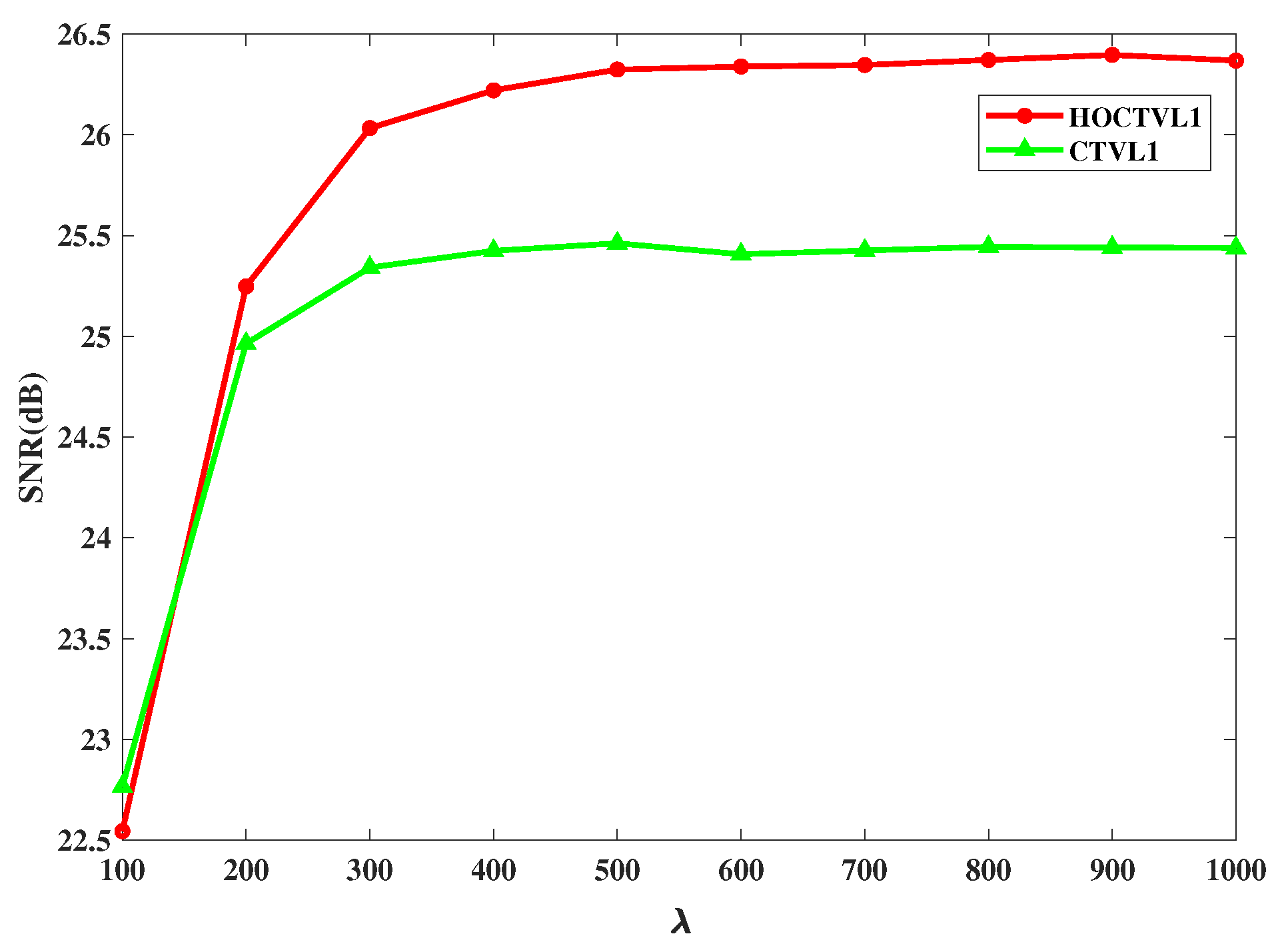Choose camera as test image and add salt-and-pepper noise with noise level 30%, the blurring kernel is Gaussian (hsize = 7, standard deviation = 5). When setting $\lambda =500$ (not the most appropriate $\lambda$) and varying ${\beta }_3$ from 500 to 30,000, the trend of SNR of the restored image is shown in Figure 4. From Figure 4, it can be seen that with the increasing of ${\beta }_3$, SNR is also increasing, and when ${\beta }_3>\mathrm{20,000}$, the trend keeps stable. In order to obtain good numerical results, in this paper, we set ${\beta }_3=\mathrm{25,000}$.

Figure 4. The SNR for results with different ${\beta }_3$.

Then considering the selection of $\lambda$, it is often a troublesome thing. In most cases, scholars obtain the appropriate $\lambda$ through experience or a lot of attempts. In [24], Gong defined a selection scheme of $\lambda$ based on numerical experiments, which is expressed as follows.

$$\lambda =\frac{c{\lambda }^{*}}{1-r}$$

(32)

where ${\lambda }^{*}$ denotes the “best” $\lambda$ found for TVL1 model, c is a constant and r represents the noise level. It means that we still need to struggle for the $\lambda$ of TVL1 model. Through a large number of simulation experiments, we find that the difficulty in selecting $\lambda$ mainly lies in the initial value of $\lambda$ when the noise level is 10%, and as the noise increases, the value of $\lambda$ decreases. Figure 5 shows the results of HOCTVL1 model and CTVL1 model corrupted by 10% salt-and-pepper noise with different $\lambda$ and it can be seen that the appropriate $\lambda$ for HOCTVL1 is almost the same with the $\lambda$ for CTVL1. Therefore, similarly, we can adopt the $\lambda$ for CTVL1 model in our HOCTVL1 model, and we set $\lambda =800$ for impulse noise with noise level 10%.

Figure 5. The SNR of HOCTVL1 and CTVL1 with different $\lambda$.

The size of local window $\omega$ is a factor that may influence the noise removal effect of SAHOCTVL1 model. In [33], the author illustrated through experiments that it can reduce more noise and recover more details when $\omega \ge 11$. Here, we also make an experiment. We choose camera as test image, and add 30% salt-and-pepper noise. When varying $\omega$ from 3 to 31, the SNR of the restored image is shown in Figure 6. From Figure 6, generally speaking, SNR does not change much, and when $\omega \ge 13$, SNR tends to be stable. Therefore, in this paper, we still set $\omega =21$ and the other parameters are the same as mentioned before.

Figure 6. The SNR for results with different $\omega$.

5.2. Convergence Analysis of HOCTVL1 Model

In this subsection, the convergence of HOCTVL1 algorithm will be analyzed. In [23], the author has proved that the CTVL1 model can converge to an optimal solution and its dual. Let $\left\{{\mathit{y}}^k,{\mathit{w}}^k,{\mathit{z}}^k,{\mathit{x}}^k,{{\mathit{\mu }}_1}^k,{{\mathit{\mu }}_2}^k,{{\mathit{\mu }}_3}^k\right\}$ be the iterative sequence generated by the ADMM approach, and set $Q_1(y)={\displaystyle \sum _{1\le i,j\le n}}{∥y_{i,j}∥}_2$, $Q_2(w)={\displaystyle \sum _{1\le i,j\le n}}{∥w_{i,j}∥}_2$, $Q_3(z)=\lambda ({∥z∥}_1-⟨F(\tilde{z}),z⟩)$. It is obvious that $Q_1:R^{2n^2}\to R$, $Q_2:R^{4n^2}\to R$, and $Q_3:R^{n^2}\to R$ are closed proper convex functions. Then according to the subsection 4.3 of [23], it is easy for us to obtain the convergence result of HOCTVL1 model. Here, we verify the convergence property of HOCTVL1 model from another point of view. We observe the changes of SNR and $\mathit{F}(\mathit{z})$ with the iterations by considering the camera image of size of $256\times 256$ corrupted by Gaussian blur (hsize = 15, standard deviation = 5) and 50% salt-and-pepper noise, $\lambda =500$, as are shown in Figure 7.

Figure 7. Changes of SNR and $F(z)$ with the iterations for Camera image corrupted by Gaussian blur and 50% salt-and-pepper noise. (a) SNR; (b) $F(z)$.

It can be seen that the SNR value (or the function $\mathit{F}(\mathit{z})$) increases (or decreases) monotonically, which can demonstrate the convexity of the model. Besides, it can be seen that after 130th iteration, the SNR values keep stable, and the function remains unchanged after 70th iteration, which means that the model has converged to an optimal solution.

5.3. Comparisons of TVL1, HTVL1 and CTVL1 Models

In this subsection, some experiments are made to illustrate the superiority of HOCTVL1 model in removing the impulse noise and overcoming the staircase effects. By comparing the restoration effect of TVL1, HTVL1 and CTVL1 models, the superiority of our model is further illustrated. For CTVL1 model and HOCTVL1 model, the results of TVL1 model are used as the initial value, and the initial value is same. The blurring kernel is Gaussian (hsize = 15, standard deviation = 5). Next, the experiments will be carried out from three aspects: (1) Deblurring image under salt-and-pepper noise. (2) Deblurring image under random-valued noise. (3) Analysis of convergence rate.

5.3.1. For Salt-and-Pepper Noise

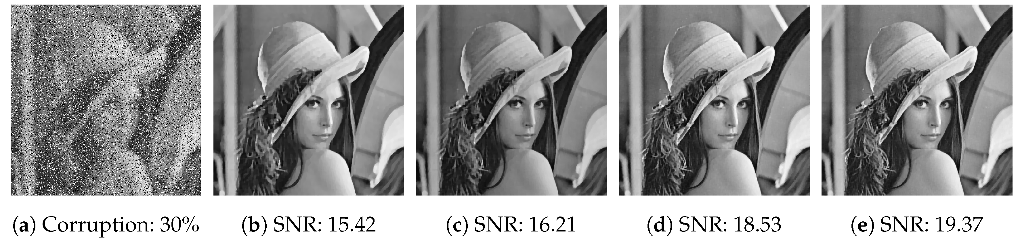
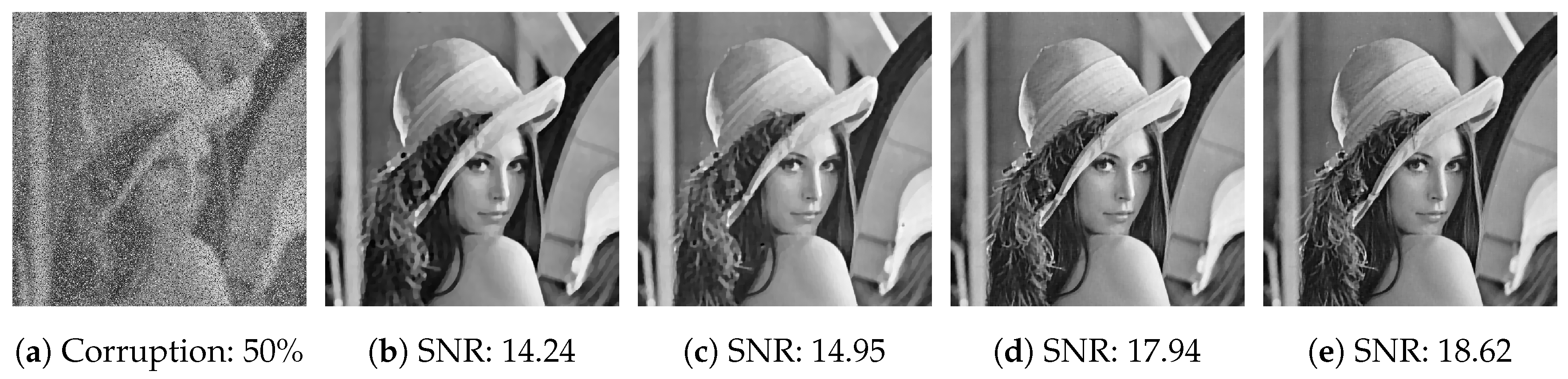
Firstly, the visual comparisons of Lena image corrupted by Gaussian blur and salt-and-pepper noise with noise levels 30%, 50%, 70% are carried out, and the results are shown in Figure 8, Figure 9 and Figure 10 respectively. The unit of SNR value is dB.

Figure 8. Comparisons of TVL1, HTVL1, CTVL1 and HOCTVL1 model on the Lena image corrupted by Gaussian blur and salt-and-pepper noise with noise level 30%. (a) Corrupted image. (b) TVL1 model. (c) HTVL1 model. (d) CTVL1 model. (e) HOCTVL1 model.

Figure 9. Comparisons of TVL1, HTVL1, CTVL1 and HOCTVL1 model on the Lena image corrupted by Gaussian blur and salt-and-pepper noise with noise level 50%. (a) Corrupted image. (b) TVL1 model. (c) HTVL1 model. (d) CTVL1 model. (e) HOCTVL1 model.

Figure 10. Comparisons of TVL1, HTVL1, CTVL1 and HOCTVL1 model on the Lena image corrupted by Gaussian blur and salt-and-pepper noise with noise level 70%. (a) Corrupted image. (b) TVL1 model. (c) HTVL1 model. (d) CTVL1 model. (e) HOCTVL1 model.

From Figure 8, Figure 9 and Figure 10, it can be found that for noise levels 30% and 50%, four models can all remove the salt-and-pepper noise effectively, but the quality of the restored images is different. The restored image by HOCTVL1 model is closer to the original image and its SNR is the highest. For noise level 70%, the restored image by TVL1 model is not clear. The restored image by HTVL1 model is clearer than the restored image by TVL1 model, but there are some noise points in the image that have not been removed, while both CTVL1 model and HOCTVL1 model can get a good restored result. By comparing the results of TVL1 model and HTVL1 model, the image quality can be indeed improved by introducing the high-order TV regularizer term. However, since the poor performance of TVL1 model, the results of HTVL1 is not very good. Since an adaptive correction procedure is introduced in CTVL1 model, which can greatly enhance the effect of image deblurring. While we combine the CTVL1 model with second-order TV regularizer term, which can further improve the effect of image deblurring. Both for removing the salt-and-pepper noise with noise level from 30% to 70%, HOCTVL1 model can have a great performance. It cannot only provide a very good visual effect, but also achieve a higher SNR. Especially for noise level 30%, the SNR value of the restored image by HOCTVL1 model is more than 1 dB higher than that by CTVL1 model and for noise level 50%, the SNR value obtained by HOCTVL1 model is also about 0.6 dB higher than CTVL1 model.

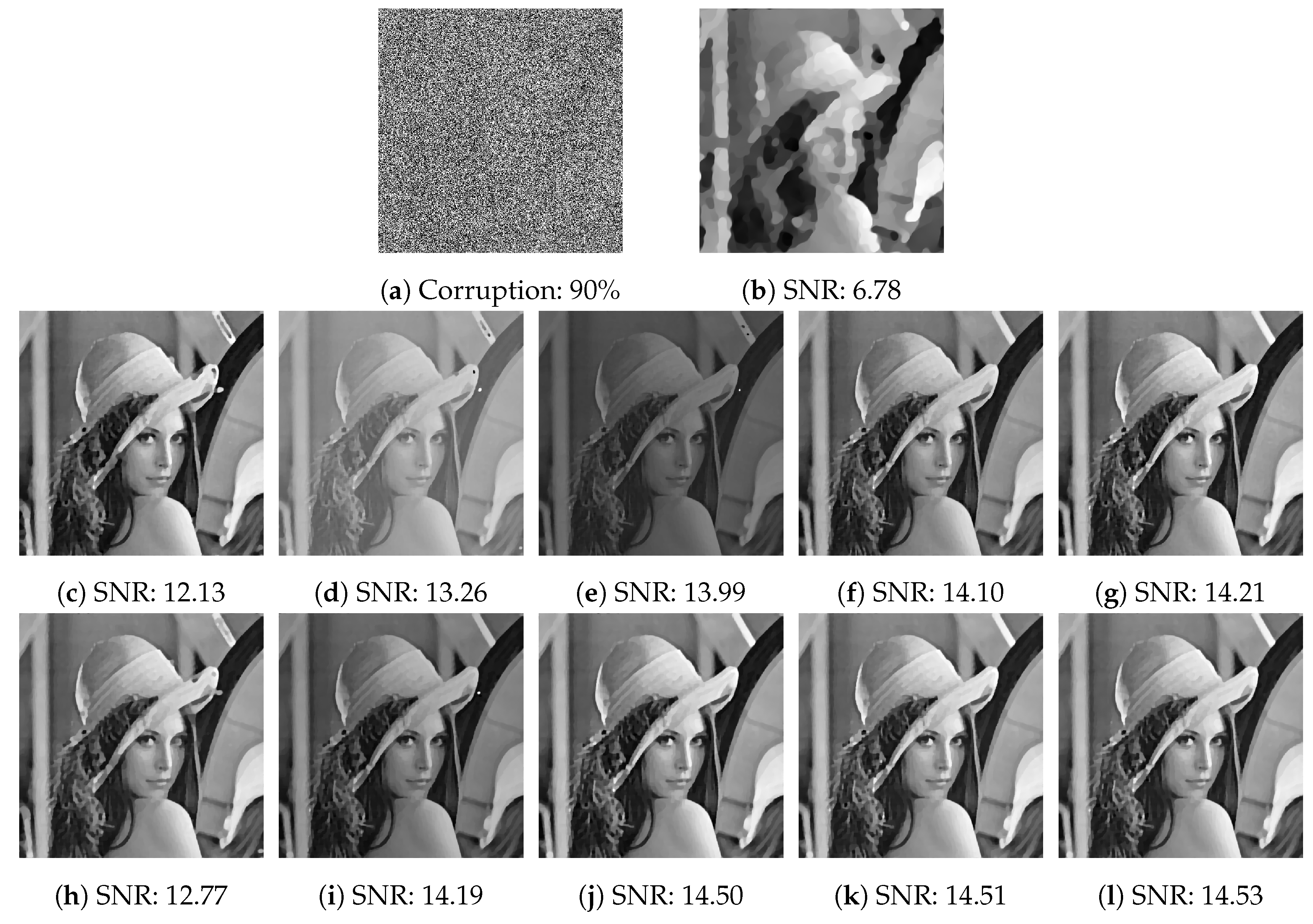
For noise level 90%, HOCTVL1 model can also use the step correction to improve the removal effect, as shown in Figure 11. Figure 11 shows the results of CTVL1 model and HOCTVL1 model during five correction steps. It can be seen that after several correction steps, two models both can improve the effect of image deblurring though the effect of TVL1 model is worse. However, from first correction step to fifth correction step, the SNR of our HOCTVL1 model is always higher than CTVL1 model. After first correction step, the SNR of recovered image by HOCTVL1 model is about 0.6 dB higher than CTVL1 model. Meanwhile, after three correction steps, the SNR of the restored image keeps stable, and the noise is eliminated, which shows that the correction efficiency of HOCTVL1 model is very high.

Figure 11. Restored images of TVL1, CTVL1 and HOCTVL1 models on the Lena image corrupted by Gaussian blur and salt-and-pepper noise with noise level 90%. (a) Corrupted image. (b) TVL1 model. (c–g) first correction step to fifth correction step of CTVL1 model. (h–l) first correction step to fifth correction step of HOCTVL1 model.

Table 1 shows the results of the four models for restoring the corrupted images with noise levels 10%, 30%, 50%, 70% and 90%. The test images are what are shown in Figure 3. It should be noted that the values of CTVL1 and HOCTVL1 model for noise level 90% are the SNR of the restored images after first correction step. From Table 1, it can be seen that compared with other three models, HOCTVL1 model can achieve a higher SNR value. It can also be seen that there is a great improvement in HOCTVL1 model compared with TVL1 and HTVL1 model no matter what the noise level is. Compared with CTVL1 model, there is about 1 dB higher in restoring the Lena, pepper and boat images when noise levels are 10% and 30%. Even for recovering camera image, the SNR of the restored image by HOCTVL1 model is still at least 0.5 dB higher than CTVL1 model when noise levels are 10% and 30%. For noise level 90%, the SNR of our HOCTVL1 model is the highest among the four model, though there is only a slight improvement in the camera image.

Table 1. SNR of four different models for test images corrupted by Gaussian blur and salt-and-pepper noise.

Image	Noise Level	SNR(dB)
		TVL1	HTVL1	CTVL1	HOCTVL1
Lena	10%	15.68	16.83	18.93	19.79
	50%	14.82	15.14	18.01	18.60
	70%	12.39	13.59	17.43	17.71
	90%	7.32	6.77	12.13	12.77
Camera	10%	12.95	13.64	16.27	16.92
	30%	12.30	12.99	15.73	16.21
	50%	11.48	11.79	14.79	15.28
	70%	10.26	10.27	12.44	12.54
	90%	5.73	5.56	8.08	8.20
Pepper	10%	19.40	21.65	25.08	26.00
	30%	18.96	21.01	24.24	25.43
	50%	17.98	19.31	23.65	24.63
	70%	16.14	16.48	22.77	23.25
	90%	7.90	7.12	13.16	14.75
Boat	10%	15.26	16.54	19.03	20.02
	30%	14.78	16.01	18.58	19.52
	50%	13.63	14.58	18.08	18.69
	70%	12.30	12.51	17.26	17.69
	90%	6.79	6.13	10.99	11.36

5.3.2. For Random-Valued Noise

For the sake of testing the performance of HOCTVL1 model in removing random-valued noise, we also carry out a series of experiments. Figure 12 and Figure 13 show the visual comparisons of Lena image corrupted by Gaussian blur and random-valued with noise levels 30% and 50%. It can be seen that for noise level 30%, both four models can effectively restore the corrupted image, but the image restored by TVL1 is still somewhat blurred, the images recovered by other three models are clearer and the recovered image by HOCTVL1 model is closer to the original image and its SNR is the highest. For noise level 50%, there is a little noise in Figure 13b,c, which shows that TVL1 and HTVL1 models cannot completely remove the 50% random-valued noise though HTVL1 model has a better performance. While CTVL1 model and HOCTVL1 model can remove noise very well, and the recovered image by HOCTVL1 model is clearer than that by CTVL1 model, which illustrates that high-order regularizer term can effectively restrain the staircase effects. Meanwhile, the value of SNR of HOCTVL1 model also illustrates this point.

Figure 12. Comparisons of TVL1, HTVL1, CTVL1 and HOCTVL1 model on the Lena image corrupted by Gaussian blur and random-valued noise with noise level 30%. (a) Corrupted image. (b) TVL1 model. (c) HTVL1 model. (d) CTVL1 model. (e) HOCTVL1 model.

Figure 13. Comparisons of TVL1, HTVL1, CTVL1 and HOCTVL1 model on the Lena image corrupted by Gaussian blur and random-valued noise with noise level 50%. (a) Corrupted image. (b) TVL1 model. (c) HTVL1 model. (d) CTVL1 model. (e) HOCTVL1 model.

Figure 14 shows the results of TVL1, five correction steps of CTVL1 model and eighth correction steps of HOCTVL1 model for removing the random-valued noise with noise level 70%. Though the performance of TVL1 model is not good, after several correction steps, both CTVL1 model and HOCTVL1 model can improve the restoration effect. Meanwhile, it can be found that the SNR of the new model is always higher than CTVL1 model after the same correction step. Besides, after the eighth correction step, there are only a few noise points in the image and the restored image is very clear, which shows the superiority of HOCTVL1 model.

Figure 14. Restored images of TVL1, CTVL1 and HOCTVL1 model on the Lena image corrupted by Gaussian blur and random-valued noise with noise level 70%. (a) Corrupted image. (b) TVL1 model. (c–g) first correction step to fifth correction step of CTVL1 model. (h–o) first correction step to eighth correction step of HOCTVL1 model.

Table 2 shows the results of the four models for restoring the corrupted images with noise levels 10%, 30%, 50%, 70%. The values of CTVL1 and HOCTVL1 models for noise level 70% in Table 2 are also the SNR of the restored images after first correction step. The values show the superiority of our model for removing the random-valued noise. Different to removing salt-and-pepper noise, there is only a little improvement compared to CTVL1 model for removing noise as high as 70%. But when the noise level is lower than 70%, the improvement is remarkable.

Table 2. SNR of four different models for test images corrupted by Gaussian blur and random-valued noise.

Image	Noise Level	SNR(dB)
		TVL1	HTVL1	CTVL1	HOCTVL1
Lena	10%	15.70	16.82	18.87	19.68
	30%	15.41	16.25	18.48	19.32
	50%	14.24	14.95	17.94	18.62
	70%	8.34	8.28	9.35	9.54
Camera	10%	12.97	13.64	16.22	16.76
	30%	12.18	12.88	15.80	16.20
	50%	9.35	9.37	11.20	11.46
	70%	3.30	3.60	3.63	3.79
Pepper	10%	19.41	21.57	25.00	25.95
	30%	18.94	20.88	24.24	25.35
	50%	16.23	16.88	20.88	21.40
	70%	7.58	7.12	8.63	8.80
Boat	10%	15.26	16.48	19.01	19.90
	30%	14.76	15.94	18.55	19.47
	50%	12.90	13.62	17.06	18.31
	70%	6.57	7.06	7.88	7.98

5.3.3. Analysis of Convergence Rate

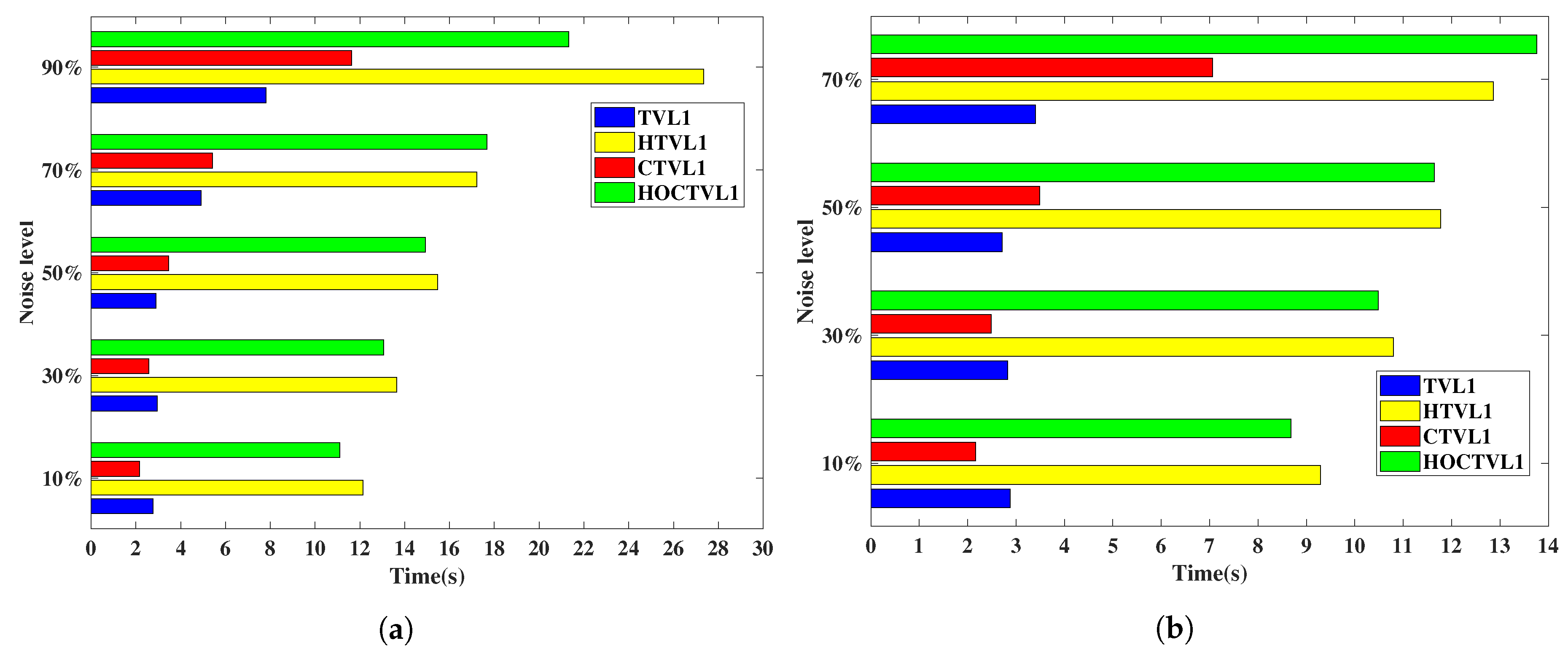
Now, we analyze the convergence rate of four models. We choose Lena as the test image, and use the running time to evaluate the convergence rate. Figure 15 shows the time that four models spend restoring the corrupted Lena image under impulse noise with different level. It can be seen that when dealing with the same noise, TVL1 and CTVL1 model cost relatively less time. Because of the combination of high-order TV regularizer term, which increases the computational complexity of the algorithm, HTVL1 and HOCTVL1 models consume more time compared to TVL1 and CTVL1 model. While HOCTVL1 model can effectively reduce the staircase effect and restore more details, it is worthwhile taking more time. Figure 16 shows the change of $F(z)$ with the iteration number when dealing with the salt-and-pepper noise with noise levels 30% and 50%. It can be seen that the convergence rate of HOCTVL1 model is slower than CTVL1 model, and the iteration number is about twice as much as that of CTVL1 model.

Figure 15. Running time of four different models for Lena corrupted by Gaussian blur and impulse noise. (a) Salt-and-pepper noise; (b) Random-valued noise.

Figure 16. Change of $F(z)$ value with Iteration number. (a) Corruption: 30%; (b) Corruption: 50%.

5.4. Comparisons of Some Other Methods

In this subsection, we compare the effect of the HOCTVL1 model with some other methods for image deblurring under impulse noise, mainly include: LpTV-ADMM [26], AOP [41], PDA [42] and L0TV-PADMM [43]. Since in [23], the author has shown the superiority of CTVL1 model by numerical experiments compared with two-phase method, in this subsection, we do not consider two-phase method. In this experiment, for ease of comparison, we choose “Gaussian” blurring kernel with hsize =9 and standard deviation =7, which is same with [43] and the parameter settings of these methods also obey to the related papers and readers can refer to them for details.

Firstly, we show the visual results of the pepper image corrupted by salt-and-pepper noise and random-valued noise with noise level 50% respectively, as are shown in Figure 17 and Figure 18.

Figure 17. Recovered images on Pepper image corrupted by salt-and-pepper noise with noise level 50%. (a) Corrupted image. (b) Lp-ADMM. (c) AOP. (d) PDA. (e) L0TV-PADMM. (f) HOCTVL1.

Figure 18. Recovered images on Pepper image corrupted by random-valued noise with noise level 50%. (a) Corrupted image. (b) Lp-ADMM. (c) AOP. (d) PDA. (e) L0TV-PADMM. (f) HOCTVL1.

From Figure 17 and Figure 18, it can be seen that the restoration effect of HOCTVL1 model is very remarkable. It is obvious that HOCTVL1 model has the highest SNR, followed by PDA and AOP methods, and the Lp-ADMM method has the lowest SNR. When removing 50% salt-and-pepper noise, as shown in Figure 17, compared with Lp-ADMM method, the SNR of (f) is more than twice as (b). Compared with L0-PADMM method, the SNR of our model is also 4 dB higher. When removing 50% random-valued noise, compared with L0-PADMM method, our model has only about 2 dB improvement in SNR, which is less than that in removing salt-and-pepper noise. But similarly, compared with Lp-ADMM method, our model has more than 100% improvement.

Table 3 shows the results of the five methods for restoring the corrupted images by impulse noise with different noise level, respectively. The value on the left of “/” represents the result after the first correction step and the value on the right of “/” represents the result after multi-correction steps. For removing salt-and-pepper noise, it is obvious that Lp-ADMM and PDA methods perform poorly, and when noise level is 90%, Lp-ADMM method has the worst effect. When the noise level varies from 30% to 70%, HOCTVL1 model has the highest SNR in most cases, except the SNR of L0TV-PADMM when dealing with the camera image with noise level 70%. It can also be seen that L0TV-PADMM method has the best restoration effect and its SNR value is higher than our model when the noise level is 90%. For dealing with random-valued noise, it can be seen that our model has the highest SNR when noise level varies from 30% to 50%. Similarly, for noise level 70%, L0TV-PADMM method has certain advantages; however, it can be seen from Lena and boat images that our model can achieve a higher SNR than L0TV-PADMM method after multi-correction steps.

Table 3. SNR of five methods for test images corrupted by Gaussian blur and impulse noise.

Image	Algorithm	Salt-and-Pepper Noise				Random-Valued Noise
		30%	50%	70%	90%	30%	50%	70%
Lena	Lp-ADMM	14.18	12.72	8.25	2.21	14.24	12.79	7.21
	AOP	14.75	14.34	13.79	13.18	14.49	14.03	5.56
	PDA	14.22	13.75	12.96	9.12	14.07	13.41	11.77
	L0TV-PADMM	19.41	18.62	17.46	15.02	18.14	16.92	15.31
	HOCTVL1	23.66	22.19	18.52	11.05/13.82	23.49	19.44	9.27/17.24
Camera	Lp-ADMM	9.46	8.37	3.92	−0.43	9.43	7.54	2.68
	AOP	11.32	10.63	9.52	8.37	11.08	8.65	2.57
	PDA	9.91	9.57	8.98	5.86	9.64	8.92	6.54
	L0TV-PADMM	15.57	14.32	12.63	9.74	13.16	12.35	10.53
	HOCTVL1	22.27	17.89	12.55	6.22/6.46	21.67	14.79	3.65/9.51
Pepper	Lp-ADMM	16.63	14.33	7.80	1.92	16.75	13.80	6.52
	AOP	17.33	16.97	16.31	15.32	17.24	16.23	5.74
	PDA	16.53	15.95	14.91	9.54	16.30	15.45	13.10
	L0TV-PADMM	26.18	24.62	21.55	17.53	22.66	20.82	18.00
	HOCTVL1	32.07	30.64	22.58	9.80/11.25	30.34	22.94	8.06/16.09
Boat	Lp-ADMM	12.28	11.13	7.16	1.99	12.22	10.95	6.18
	AOP	13.70	12.80	12.24	11.43	13.11	12.51	5.43
	PDA	12.38	11.91	11.18	8.29	12.32	11.76	10.43
	L0TV-PADMM	19.45	18.12	16.58	13.26	17.38	15.76	14.04
	HOCTVL1	24.21	22.55	18.15	9.25/10.85	23.84	18.46	7.91/15.45

Figure 19 shows the running time of the five methods for restoring the corrupted pepper image. When dealing with 90% salt-and-pepper noise and 70% random-valued noise, HOCTVL1 model needs multi-correction steps, which costs a lot time, here we only show the time of removing salt-and-pepper noise as high as 70% and random-valued noise as high as 50%. It can be seen that compared to other four methods, our HOCTVL1 model spends the least time whatever the noise level is. It can also be found that the other four methods take several times as much time as our model, which illustrates the advantages of our model.

Figure 19. Running time of five methods for pepper corrupted by Gaussian blur and impulse noise. (a) Salt-and-pepper noise; (b) Random-valued noise.

5.5. Comparisons between SAHOCTVL1 Model and HOCTVL1 Model

In this subsection, the restoration effect of SAHOCTVL1 model will be analyzed. We choose camera and Lena as test images, we use “Gaussian” blurring with hsize = 15 and standard deviation = 5, and we set the spatially adapted iteration number $p\le 3$. Since we have shown the superiority of HOCTVL1 model by many simulation experiments, here we only compare the effect of SAHOCTVL1 model and HOCTVL1 model on image restoration. Meanwhile, since we have shown the huge advantage of HOCTVL1 model compared to HTVL1 model, while the effect of SAHTVL1 model is similar to HTVL1 model, therefore we do not consider SAHTVL1 model in [31] either. In this subsection we do not consider the 90% salt-and-pepper noise and 70% random-valued noise since the multi-correction steps take much time. We evaluate the results by SNR and running time, and the restoration results are shown in Table 4.

Table 4. Comparisons of SAHOCTVL1 and HOCTVL1 model for Cameraman and Lena corrupted by Gaussian blur and impulse noise.

Image	Noise Type	Noise Level	SNR(dB)		Time(s)
			HOCTVL1	SAHOCTVL1	HOCTVL1	SAHOCTVL1
Camera	SP	10%	16.85	16.98	2.32	6.76
		30%	16.18	16.51	2.67	8.20
		50%	15.33	15.72	3.02	9.32
		70%	12.50	12.57	5.15	15.47
	RV	10%	16.73	16.78	2.06	6.07
		30%	16.22	16.34	2.30	7.08
		50%	11.39	11.99	3.02	8.74
Lena	SP	10%	19.78	19.82	11.19	31.45
		30%	19.35	19.44	13.97	39.27
		50%	18.63	18.78	16.13	47.12
		70%	17.72	17.85	18.82	55.57
	RV	10%	19.68	19.72	9.18	30.60
		30%	19.29	19.32	11.39	36.77
		50%	18.56	18.68	12.07	41.35

SP denotes salt-and-pepper noise and RV denotes random-valued noise.

From Table 4, as is shown, generally speaking, SAHOCTVL1 model can achieve at least the same effect as HOCTVL1 model. For camera image, when noise is 30% and 50% salt-and-pepper noise, the SNR of SAHOCTVL1 model is about 0.4 dB higher than HOCTVL1 model and when noise is 50% random-valued noise, there is 0.6 dB higher than HOCTVL1 model. For Lena image, the advantage of SAHOCTVL1 model is little, and the SNR improves by about 0.1 dB when noise levels are 50% and 70%. Meanwhile, because we set $p\le 3$, which makes the algorithm run 3 times, making the time SAHOCTVL1 model takes be about 3 times as much as that HOCTVL1 model takes. But we think it is worthwhile to obtain high SNR at the expense of running time.

6. Conclusions

This paper gives a contribution to solving the problem of image deblurring under impulse noise, and two models named HOCTVL1 model and SAHOCTVL1 model are proposed. Benefitting from the merits of high-order TV regularizer term and spatially adapted regularization parameter selection scheme, both models perform well in recovering the corrupted images. A great quantity of experiments is carried out to show the superiority of the two models. Compared to CTVL1 model, HOCTVL1 model can achieve better visual effects and higher SNR values. When dealing with salt-and-pepper noise with noise level less than 90% and random-valued noise with noise level less than 70%, there is about 0.5∼1 dB improvement. When dealing with 90% salt-and-pepper noise and 70% random-valued noise, multi-correction steps are used to improve the restoration quality. HOCTVL1 model outperforms CTVL1 model both in the SNR value of each correction step and the number of correction steps they need. Compared to four other state-of-the-art methods, HOCTVL1 model always outperforms Lp-ADMM, AOP, and PDA methods. Compared to L0TV-PADMM method, HOCTVL1 model performs well in most cases and it can achieve about 1∼4 dB improvement. When dealing with 90% salt-and-pepper noise and 70% random-valued noise, L0TV-PADMM method performs well, while after several correction steps, HOCTVL1 model can obtain higher SNR value in some cases and HOCTVL1 model takes less time. In the last experiment, the comparisons of HOCTVL1 model and SAHOCTVL1 model are conducted and the results show that SAHOCTVL1 can achieve about 0.1∼0.6 dB improvement compared to HOCTVL1 model. However, it takes about three times as long as HOCTVL1 model, which is a problem that needs to be optimized in a future study.