A Robust Semi-Blind Receiver for Joint Symbol and Channel Parameter Estimation in Multiple-Antenna Systems

Abstract

For multiple-antenna systems, the technologies of joint symbol and channel parameter estimation have been developed in recent works. However, existing technologies have a number of problems, such as performance degradation and the large cost of prior information. In this paper, a tensor space-time coding scheme in multiple-antenna systems was considered. This scheme allowed spreading, multiplexing, and allocating information symbols associated with multiple transmitted data streams. We showed that the received signal was formulated as a third-order tensor satisfying a Tucker-2 model, and then a robust semi-blind receiver was developed based on the optimized Levenberg–Marquardt (LM) algorithm. Under the assumption that the instantaneous channel state information (CSI) is unknown at the receiving end, the proposed semi-blind receiver jointly estimates the information symbol and channel parameters efficiently. The proposed receiver had a better estimation performance compared with existing semi-blind receivers, and still performed well when the channel became strongly correlated. Moreover, the proposed semi-blind receiver could be extended to the multi-user massive multiple-input multiple-output (MIMO) system for joint symbol and channel estimation. Computer simulation results were shown to demonstrate the effectiveness of the proposed receiver.

1. Introduction

Multiple-antenna techniques are well known to provide spatial diversity and multiplexing gains [1,2,3]. Over the last few decades, the benefits of multiple-antenna communications have been verified in both theory and practice. On the other hand, tensor-based signaling approaches that utilize several signal dimensions such as time, space, and code, are seen as good technologies for improving the information transmission rate and enhancing communication reliability [4,5,6]. Against this background, the problem of joint symbol and channel estimation is resolved by using tensor-based signaling approaches, and a number of semi-blind or blind receivers have been proposed for multiple-input multiple-output (MIMO) systems.

A parallel factor (PARAFAC) [7] based receiver is proposed in [8] by using the Khatri–Rao space-time (KRST) coding scheme, which can achieve a flexible tradeoff between error performance and transmission efficiency. In [9], the authors extend the KRST coding scheme by using the linear constellation precoding, and then developing several semi-blind receivers. These semi-blind receivers allow a joint symbol and channel estimation without requiring pilot sequences for the instantaneous channel state information (CSI) acquisition. In [10], the authors develop a new tensor-based receiver in MIMO relay systems for channel estimation by using PARAFAC analysis. A low complexity PARAFAC-based channel estimation scheme for non-regenerative MIMO relay systems is developed in [11]. In [12], a novel semi-blind receiver is derived using a multiple KRST coding scheme for joint symbol and channel estimation. More recently, a nested PARAFAC-based receiver for cooperative MIMO communications is proposed in [13], and three-step and double two-step alternating least squares (ALS) algorithms are proposed to fit the nested PARAFAC model for estimating system parameters. For millimeter wave (mmWave) massive MIMO systems, a PARAFAC decomposition-based algorithm is developed in [14] to jointly estimate channel parameters of multiple users. In [15], the algorithm in [14] is extended to mmWave MIMO orthogonal frequency division multiplexing (MIMO-OFDM) systems for channel estimation, and Cramér–Rao bound (CRB) results for channel parameters are also derived. Considering the channel estimation issue in the presence of pilot contamination for multi-cell massive MIMO systems, a new PARAFAC-based approach is proposed in [16] to jointly estimate directions of arrival, fading coefficients, and delays. Although these works [8,9,10,11,12,13,14,15,16] consider different design approaches, their common feature is using the PARAFAC model, which needs to know the first column or row of one loading matrix to eliminate scaling ambiguity. Furthermore, the ALS algorithm used in these receivers exhibits a convergence problem when ill-conditioned factor matrices exist [17].

In contrast to the ALS algorithm, the Levenberg–Marquardt (LM) algorithm updates all the parameters to be estimated at the same time. The LM algorithm is successfully used to fit some tensor models, adapt to collinearity problems, and provide quadratic convergence [18,19,20]. A LM algorithm is first proposed for fitting PARAFAC model in [18]. In [19], the authors present a LM algorithm to the decomposition of the Block Component Model (BCM) in the uplink of a wideband direct-sequence code-division multiple access (DS-CDMA) systems. Recently, a LM algorithm was developed in [20] to jointly estimate information symbol and channel matrices for a generalized PARATUCK2 model. As an iterative algorithm, the LM algorithm is also sensitive to initialization. Thus, the optimization of the initial value is important to improve the performance of the LM algorithm.

In [21], a tensor-based space-coding scheme using PARATUCK2 model is developed. For the PARATUCK2 model, the number of channel uses can be different from one transmitted data stream to another. In [22], a generalized PARATUCK2 model is proposed by exploiting a tensor space-time (TST) coding. Recently, a Kronecker product least squares (KPLS) receiver is proposed in [23] to estimate the symbol and channel matrices. More recently, it is shown in [24] that a KPLS receiver can be extended to all the tensor-based systems. Although the KPLS receiver is a non-iterative and low-complexity solution, it needs the related core tensor unfolding to be right-invertible, which is a relatively harsh condition in signal design.

Inspired by [21] and [22], we considered a simple tensor space-time coding scheme for multiple-antenna systems, along with an efficient receiver. The allocation factor and the space-time code factor in the TST coding scheme in [22] are independent, while the allocation factor in our coding scheme is also a three-dimensional space-time code factor. Thanks to the special structure of the proposed coding scheme, the received signal can be constructed as a Tucker-2 model [25,26], which has uniqueness property under some suitable conditions. Then, a robust semi-blind receiver based on optimized LM algorithm is presented for joint channel and symbol estimation. Uniqueness and identifiability issues for the constructed Tucker-2 model are also discussed in this paper. Compared with existing receivers, the proposed receiver has a better estimation performance. Moreover, the proposed semi-blind receiver can be extended to the multi-user massive MIMO system. For the low-rank channel, the proposed receiver still has good performance for joint symbol and channel estimation even in the shorter length of code and information symbol, and larger number of data streams.

The organization of this paper is as follows. Section 2 presents a brief overview of the Tucker model. In Section 3, the system model is presented and the associated tensor signal model is formulated. Section 4 briefly reviews the receiver with the ALS algorithm and describes the proposed semi-blind receiver based on the optimized LM algorithm. Section 5 extends the proposed semi-blind receiver to multi-user massive MIMO systems for joint symbol and channel estimation. In Section 6, some simulation results are shown to demonstrate the performance of our semi-blind receiver. Conclusions are drawn in Section 7.

Notation: Scalars, vectors, matrices, and tensors are denoted by lower-case letters $\left(a,b,\cdots \right)$, boldface lower-case letters $\left(a,b,\cdots \right)$, boldface capitals $\left(A,B,\cdots \right)$, and underlined boldface capitals $\left(\underline{A},\underline{B},\cdots \right)$, respectively. $A^T$, $A^H$, $A^{-1}$, and $A^{†}$ represent transpose, conjugate transpose, inverse, and Moore–Penrose pseudo-inverse of the matrix $A$, respectively. ${∥A∥}_F$ denotes the Frobenius norm of $A$. $I_M$ denotes the $M\times M$ identity matrix. The operator $vec\left(·\right)$ stacks the columns of its matrix argument to a vector, while $unvec\left(·\right)$ represents the inverse vectorization operation. The Kronecker matrix product is denoted by ⊗. The term $D_i\left(A\right)$ corresponds the diagonal matrix out of the i-th row of $A$.

2. Tucker Model

This section first presents a brief overview of the Tucker model, and then focuses on the Tucker-2 model used in this work. For an Nth-order tensor $\underline{T}\in {\mathbb{C}}^{I_1\times \cdots \times I_N}$, a Tucker-N model or Tucker model is defined in the following scalar form as [26]:

$$\begin{array}{c}\hfill \begin{array}{c}{t}_{i_1,\dots ,i_N}={\displaystyle \sum _{r_1=1}^{R_1}}\cdots {\displaystyle \sum _{r_N=1}^{R_N}}{g}_{r_1,\dots ,r_N}\left(a_{i_1,r_1}^{\left(1\right)}\times \cdots \times a_{i_N,r_N}^{\left(N\right)}\right)\hfill \\ =\sum _{r_1=1}^{R_1}\cdots {\displaystyle \sum _{r_N=1}^{R_N}}{g}_{r_1,\dots ,r_N}{\displaystyle \prod _{n=1}^N}{a}_{i_n,r_n}^{\left(n\right)}\hfill \end{array}\end{array}$$

(1)

where $i_n=1,\dots ,I_n$ for $n=1,\dots ,N$, $a_{i_n,r_n}^{\left(n\right)}$ and $g_{r_1,\dots ,r_N}$ stand for typical elements of the matrix factor ${\mathbf{A}}^{\left(n\right)}\in {\mathbb{C}}^{I_n\times R_n}$ and the core tensor $\underline{\mathbf{G}}\in {\mathbb{C}}^{R_1\times \cdots \times R_N}$, respectively. Using the mode-n product representation, the model (1) can be written as:

$$\begin{array}{c}\hfill \begin{array}{c}\underline{\mathbf{T}}=\underline{\mathbf{G}}{\times }_1{\mathbf{A}}^{\left(1\right)}{\times }_2{\mathbf{A}}^{\left(2\right)}{\times }_3\cdots {\times }_N{\mathbf{A}}^{\left(N\right)}\hfill \\ =\underline{\mathbf{G}}{\times }_{n=1}^N{\mathbf{A}}^{\left(n\right)}\hfill \end{array}\end{array}$$

(2)

where $\underline{\mathbf{G}}{\times }_n{\mathbf{A}}^{\left(n\right)}$ denotes the mode-n product of $\underline{\mathbf{G}}$ and ${\mathbf{A}}^{\left(n\right)}$ along the $N^{th}$ mode, gives a tensor $\underline{\mathbf{W}}$ of dimensions $R_1\times \cdots \times R_{n-1}\times I_n\times R_{n+1}\times \cdots \times R_N$ such that:

$$\begin{array}{c}\hfill w_{r_1,\dots ,r_{n-1},i_n,r_{n+1},\dots ,r_N}=\sum _{r_n=1}^{R_n}{a}_{i_n,r_n}^{\left(n\right)}{g}_{r_1,\dots ,r_{n-1},r_n,r_{n+1},\dots ,r_N}\end{array}$$

(3)

where $w_{r_1,\dots ,r_{n-1},i_n,r_{n+1},\dots ,r_N}$ is a typical element of the tensor $\underline{\mathbf{W}}$. It has been known that the Tucker model is not essentially unique [26], which restricts its application. Their matrix factors can be only determined up to nonsingular transformations characterized by nonsingular matrices. However, some low-order Tucker models with special structures are unique up to permutation and/or scaling ambiguities.

Assuming $N=3$ and ${\mathbf{A}}^{\left(3\right)}={\mathbf{I}}_{I_3}$ for the third-order tensor $\underline{\mathbf{T}}\in {\mathbb{C}}^{I_1\times I_2\times I_3}$, we have:

$$\begin{array}{c}\hfill \begin{array}{c}{t}_{i_1,i_2,i_3}={\displaystyle \sum _{r_1=1}^{R_1}}{\displaystyle \sum _{r_2=1}^{R_2}}{\displaystyle \sum _{r_3=1}^{R_3}}{g}_{r_1,r_2,r_3}{\displaystyle \prod _{n=1}^3}{a}_{i_n,r_n}^{\left(n\right)}\hfill \\ ={\displaystyle \sum _{r_1=1}^{R_1}}{\displaystyle \sum _{r_2=1}^{R_2}}{g}_{r_1,r_2,i_3}{a}_{i_1,r_1}^{\left(1\right)}{a}_{i_2,r_2}^{\left(2\right)}.\hfill \end{array}\end{array}$$

(4)

This model is called Tucker-2 model or Tucker-(2, 3) model, and is widely applied in data analysis and parameter estimation [4]. ${\mathbf{A}}^{\left(1\right)}$ and ${\mathbf{A}}^{\left(2\right)}$ are the two loading matrices, and $\underline{\mathbf{G}}$ is the core tensor. In the same way, such a model can be written in terms of mode-n product as:

$$\begin{array}{c}\hfill \begin{array}{c}\underline{\mathbf{T}}=\underline{\mathbf{G}}{\times }_1{\mathbf{A}}^{\left(1\right)}{\times }_2{\mathbf{A}}^{\left(2\right)}{\times }_3{\mathbf{I}}_{I_3}\hfill \\ =\underline{\mathbf{G}}{\times }_{n=1}^2{\mathbf{A}}^{\left(n\right)}.\hfill \end{array}\end{array}$$

(5)

3. System Model

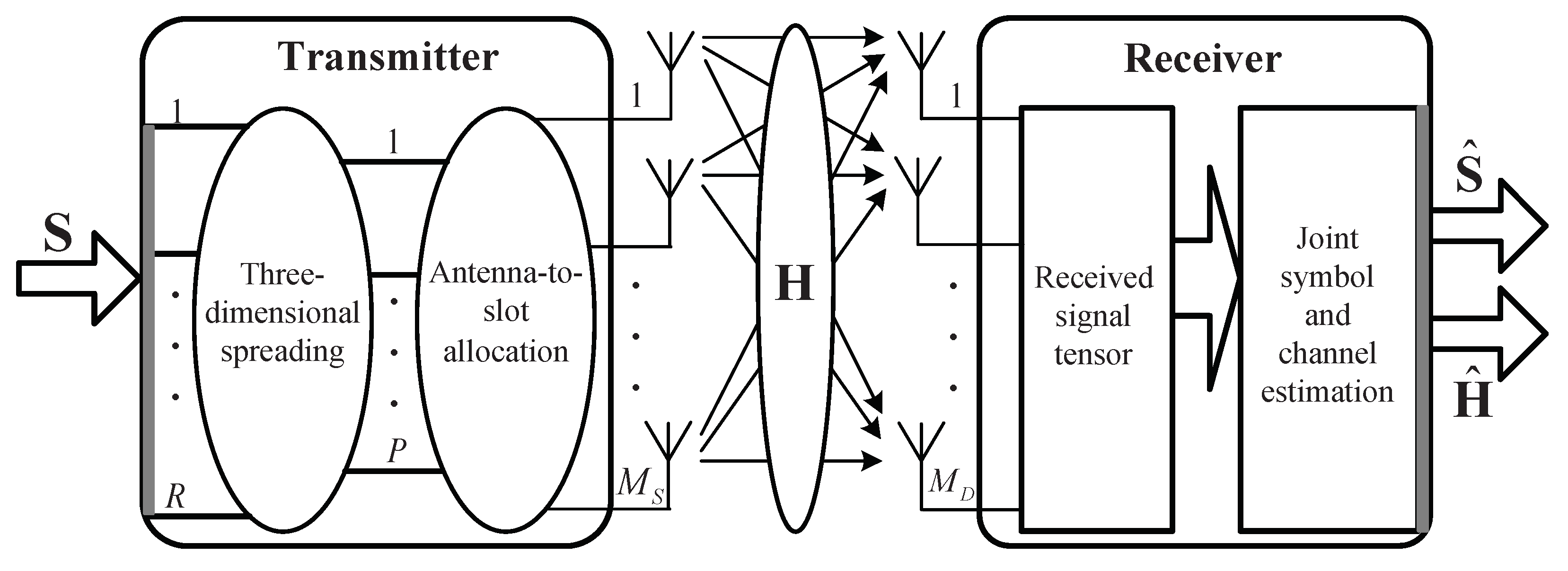
Consider a multiple-antenna system with $M_S$ transmit antennas and $M_D$ receive antennas as shown in Figure 1. $h_{m_D,m_S}$ represents the channel coefficient between the $m_S$-th transmit antenna and the $m_D$-th receive antenna ($m_S=1,\dots ,M_S$, $m_D=1,\dots ,M_D$). $s_{n,r}$ represents the n-th symbol of the r-th data stream ($n=1,\dots ,N$, $r=1,\dots ,R$), with each data stream being formed of N information symbols. Each symbol $s_{n,r}$ is coded by a three-dimensional space-time code $b_{m_S,r,p}$ ($p=1,\dots ,P$), whose dimensions are the numbers of transmit antennas, data streams, and chips, respectively. We then define the antenna-to-slot allocation factor $q_{p,m_S}$, which is 0 or 1. Both the transmitter and the receiver know these factors $b_{m_S,r,p}$ and $q_{p,m_S}$.

The signal transmitted from $m_S$-th transmit antenna, during the n-th symbol period of the p-th chip, is given by:

$$\begin{array}{c}\hfill x_{m_S,n,p}=\sum _{r=1}^R{q}_{p,m_S}{b}_{m_S,r,p}{s}_{n,r}\end{array}$$

(6)

where $s_{n,r}$ and $q_{p,m_S}$ are $\left(n,r\right)$-th and $\left(p,m_S\right)$-th elements of signal matrix $\mathbf{S}\in {\mathbb{C}}^{N\times R}$ and the antenna-to-slot allocation matrix $\mathbf{Q}\in {\mathbb{C}}^{P\times M_S}$, respectively. $x_{m_S,n,p}$ and $b_{m_S,r,p}$ are typical elements of the transmitted signal tensor $\underline{\mathbf{X}}\in {\mathbb{C}}^{M_S\times N\times P}$ and the coding tensor $\underline{\mathbf{B}}\in {\mathbb{C}}^{M_S\times R\times P}$, respectively. The elements in $\underline{\mathbf{B}}$ are chosen as $e^{\sqrt{-1}\varsigma /\phantom{\sqrt{-1}\varsigma 2\pi }2\pi }$, where $\varsigma$ is taken from random uniformly distributed pseudorandom numbers. In our tensor coding scheme, the number of transmitted data streams is not restricted to be equal to that of transmit antennas, and the data streams can be allocated to an arbitrary set of transmitted antennas. Without considering the allocation of stream-to-slot, the coding scheme in [21] can be regarded as a special case of our tensor coding scheme with a fixed two-dimensional space-time code.

Assuming Rayleigh flat fading channels, then the discrete-time baseband signal at the $m_D$-th receive antenna can be written as:

$$\begin{array}{c}\hfill \begin{array}{c}{y}_{m_D,n,p}={\displaystyle \sum _{m_S=1}^{M_S}}{h}_{m_D,m_S}{x}_{m_S,n,p}+v_{m_D,n,p}\hfill \\ ={\displaystyle \sum _{m_S=1}^{M_S}}{\displaystyle \sum _{r=1}^R}{h}_{m_D,m_S}{q}_{p,m_S}{b}_{m_S,r,p}{s}_{n,r}+v_{m_D,n,p}\hfill \end{array}\end{array}$$

(7)

where $h_{m_D,m_S}$ is the $\left(m_D,m_S\right)$-th element of channel matrix $\mathbf{H}\in {\mathbb{C}}^{M_D\times M_S}$, $y_{m_D,n,p}$ and $v_{m_D,n,p}$ are typical elements of the received signal tensor $\underline{\mathbf{Y}}\in {\mathbb{C}}^{M_D\times N\times P}$ and the noise tensor $\underline{\mathbf{V}}\in {\mathbb{C}}^{M_D\times N\times P}$, respectively.

3.1. Constructed Tucker-2 Model

Let us define $c_{m_S,r,p}=q_{p,m_S}{b}_{m_S,r,p}$, where $c_{m_S,r,p}$ is the typical element of the compound tensor $\underline{\mathbf{C}}\in {\mathbb{C}}^{M_S\times R\times P}$. So Equation (7) can be written as:

$$\begin{array}{c}\hfill y_{m_D,n,p}=\sum _{m_S=1}^{M_S}\sum _{r=1}^R{h}_{m_D,m_S}{c}_{m_S,r,p}{s}_{n,r}+v_{m_D,n,p}.\end{array}$$

(8)

By comparing Equation (4) with Equation (8), the received signal tensor $\underline{\mathbf{Y}}\in {\mathbb{C}}^{M_D\times N\times P}$ of noiseless signals satisfies a Tucker-2 model, with the following correspondences:

$$\begin{array}{c}\hfill \left(\underline{\mathbf{G}},{\mathbf{A}}^{\left(1\right)},{\mathbf{A}}^{\left(2\right)}\right)\iff \left(\underline{\mathbf{C}},\mathbf{H},\mathbf{S}\right)\end{array}$$

(9)

$$\begin{array}{c}\hfill \left(I_1,I_2,R_1,R_2,I_3\right)\iff \left(M_D,N,M_S,R,P\right).\end{array}$$

(10)

Using the mode-n product representation, the model (8) can be written as:

$$\begin{array}{c}\hfill \underline{\mathbf{Y}}=\underline{\mathbf{C}}{\times }_1\mathbf{H}{\times }_2\mathbf{S}+\underline{\mathbf{V}}\end{array}$$

(11)

where $\mathbf{S}$ and $\mathbf{H}$ represent the two loading matrices, and $\underline{\mathbf{C}}$ is the core tensor.

Let us define ${\mathbf{Y}}_{··p}\in {\mathbb{C}}^{M_D\times N}$, ${\mathbf{B}}_{··p}\in {\mathbb{C}}^{M_S\times R}$, ${\mathbf{C}}_{··p}\in {\mathbb{C}}^{M_S\times R}$ and ${\mathbf{V}}_{··p}\in {\mathbb{C}}^{M_D\times N}$ as the p-th matrix slice of $\underline{\mathbf{Y}}\in {\mathbb{C}}^{M_D\times N\times P}$, $\underline{\mathbf{B}}\in {\mathbb{C}}^{M_S\times R\times P}$, $\underline{\mathbf{C}}\in {\mathbb{C}}^{M_S\times R\times P}$, and $\underline{\mathbf{V}}\in {\mathbb{C}}^{M_D\times N\times P}$, respectively. We have ${\mathbf{C}}_{··p}=D_p\left(\mathbf{Q}\right){\mathbf{B}}_{··p}$. By defining ${\mathbf{Y}}_1={\left[{\mathbf{Y}}_{··1}^T,\dots ,{\mathbf{Y}}_{··P}^T\right]}^T\in {\mathbb{C}}^{P{M}_D\times N}$, ${\mathbf{Y}}_2={\left[{\mathbf{Y}}_{··1},\dots ,{\mathbf{Y}}_{··P}\right]}^T\in {\mathbb{C}}^{PN\times M_D}$, ${\mathbf{Y}}_3=\left[vec\left({\mathbf{Y}}_{··1}\right),\dots ,vec\left({\mathbf{Y}}_{··P}\right)\right]\in {\mathbb{C}}^{M_{D}N\times P}$, and ${\mathbf{Y}}_4=\left[vec\left({\mathbf{Y}}_{··1}^T\right),\dots ,vec\left({\mathbf{Y}}_{··P}^T\right)\right]\in {\mathbb{C}}^{N{M}_D\times P}$, we can obtain four compact forms of the Tucker-2 model (11):

$$\begin{array}{c}\hfill \begin{array}{c}{\mathbf{Y}}_1=\left({\mathbf{I}}_P\otimes \mathbf{H}\right){\mathbf{F}}_1{\mathbf{S}}^T+{\mathbf{V}}_1\end{array}\end{array}$$

(12)

$$\begin{array}{c}\hfill \begin{array}{c}{\mathbf{Y}}_2=\left({\mathbf{I}}_P\otimes \mathbf{S}\right){\mathbf{F}}_2{\mathbf{H}}^T+{\mathbf{V}}_2\end{array}\end{array}$$

(13)

$$\begin{array}{c}\hfill \begin{array}{c}{\mathbf{Y}}_3=\left(\mathbf{S}\otimes \mathbf{H}\right){\mathbf{F}}_3+{\mathbf{V}}_3\end{array}\end{array}$$

(14)

$$\begin{array}{c}\hfill \begin{array}{c}{\mathbf{Y}}_4=\left(\mathbf{H}\otimes \mathbf{S}\right){\mathbf{F}}_4+{\mathbf{V}}_4\end{array}\end{array}$$

(15)

with,

$$\begin{array}{c}\hfill \begin{array}{c}{\mathbf{F}}_1={\left[{\mathbf{B}}_{··1}^T{D}_1\left(\mathbf{Q}\right),\dots ,{\mathbf{B}}_{··P}^T{D}_P\left(\mathbf{Q}\right)\right]}^T\hfill \\ {\mathbf{F}}_2={\left[D_1\left(\mathbf{Q}\right){\mathbf{B}}_{··1},\dots ,D_P\left(\mathbf{Q}\right){\mathbf{B}}_{··P}\right]}^T\hfill \\ {\mathbf{F}}_3=\left[vec\left(D_1\left(\mathbf{Q}\right){\mathbf{B}}_{··1}\right),\dots ,vec\left(D_P\left(\mathbf{Q}\right){\mathbf{B}}_{··P}\right)\right]\hfill \\ {\mathbf{F}}_4=\left[vec\left({\mathbf{B}}_{··1}^T{D}_1\left(\mathbf{Q}\right)\right),\dots ,vec\left({\mathbf{B}}_{··P}^T{D}_P\left(\mathbf{Q}\right)\right)\right]\hfill \end{array}\end{array}$$

(16)

and,

$$\begin{array}{c}\hfill \begin{array}{c}{\mathbf{V}}_1={\left[{\mathbf{V}}_{··1}^T,\dots ,{\mathbf{V}}_{··P}^T\right]}^T\hfill \\ {\mathbf{V}}_2={\left[{\mathbf{V}}_{··1},\dots ,{\mathbf{V}}_{··P}\right]}^T\hfill \\ {\mathbf{V}}_3=\left[vec\left({\mathbf{V}}_{··1}\right),\dots ,vec\left({\mathbf{V}}_{··P}\right)\right]\hfill \\ {\mathbf{V}}_4=\left[vec\left({\mathbf{V}}_{··1}^T\right),\dots ,vec\left({\mathbf{V}}_{··P}^T\right)\right].\hfill \end{array}\end{array}$$

(17)

In this paper, two following assumptions are satisfied.

(a) The antenna-to-slot allocation matrix $\mathbf{Q}$ does not have an all-zero column. This means that at least one transmit antenna is used during each time slot;

(b) Both the transmitter and receiver know the allocation matrix $\mathbf{Q}$ and the coding tensor $\underline{\mathbf{B}}$.

3.2. Uniqueness Issue

Due to the loading matrices factors being unique up to nonsingular matrices, the generalized Tucker-2 model is not essentially unique. This consequence can be verified by using the property of the mode-n product:

$$\begin{array}{c}\hfill \begin{array}{c}\underline{\mathbf{C}}{\times }_1\mathbf{H}{\times }_2\mathbf{S}=\underline{\mathbf{C}}{\times }_1\left(\mathbf{H}{\Theta }_{\mathbf{H}}{\Theta }_{\mathbf{H}}^{-1}\right){\times }_2\left(\mathbf{S}{\Theta }_{\mathbf{S}}{\Theta }_{\mathbf{S}}^{-1}\right)\hfill \\ =\underline{\mathbf{C}}{\times }_1{\Theta }_{\mathbf{H}}^{-1}{\times }_2{\Theta }_{\mathbf{S}}^{-1}{\times }_1\left(\mathbf{H}{\Theta }_{\mathbf{H}}\right){\times }_2\left(\mathbf{S}{\Theta }_{\mathbf{S}}\right)\hfill \end{array}\end{array}$$

(18)

where the noise tensor $\underline{\mathbf{V}}$ has been omitted for convenience of notation, ${\Theta }_{\mathbf{S}}\in {\mathbb{C}}^{R\times R}$ and ${\Theta }_{\mathbf{H}}\in {\mathbb{C}}^{M_S\times M_S}$ are nonsingular matrices.

It is shown that applying the uniqueness theorem of the Tucker model in [25], if the core tensor $\underline{\mathbf{C}}$ is known, then $\mathbf{S}$ and $\mathbf{H}$ are unique to a scaling ambiguity, i.e.,

$$\begin{array}{c}\hfill \left(\mathbf{S},\mathbf{H}\right)=\left({\overline{\mathbf{S}}\Theta }_{\mathbf{S}}^{-1},{\overline{\mathbf{H}}\Theta }_{\mathbf{H}}^{-1}\right)\end{array}$$

(19)

where $\overline{\mathbf{S}}$ and $\overline{\mathbf{H}}$ are alternative solutions for $\mathbf{S}$ and $\mathbf{H}$, respectively, ${\Theta }_{\mathbf{S}}=\beta {\mathbf{I}}_R$ and ${\Theta }_{\mathbf{H}}=\left(1/\phantom{1\beta }\beta \right){\mathbf{I}}_{M_S}$. Consequently, the priori knowledge of only one symbol is enough to resolve this scaling ambiguity factor $\beta$. Compared to the PARAFAC model used in existing receivers, the constructed Tucker-2 model only needs a priori knowledge of one symbol to eliminate the scaling ambiguity. Therefore, our scheme has higher spectral efficiency.

3.3. Identifiability Conditions

The identifiability for the constructed Tucker-2 model is an assignable problem for recovering the parameters to be estimated. In this paper, it is directly linked to the estimation of the signal matrix $\mathbf{S}$ and channel matrix $\mathbf{H}$ from the received signal tensor $\underline{\mathbf{Y}}$. Conditions of parameter identifiability is given in the following theorem.

Theorem 1.

(Sufficient Conditions): Assuming that $\mathbf{H}$ has independent and identically distributed (i.i.d.) entries, and $\mathbf{S}$ has a full column rank. $P_1$ denotes the number of nonzero elements in $\mathbf{Q}$. Then sufficient conditions for identifiability of signal matrix $\mathbf{S}$ and channel matrix $\mathbf{H}$ are:

$$P_1⩾Randmin\left(M_D,R\right)⩾M_S.$$

(20)

Proof of Theorem 1.

From Equation (12) and Equation (13), necessary and sufficient conditions for identifiability of $\mathbf{S}$ and $\mathbf{H}$ requires that $\left({\mathbf{I}}_P\otimes \mathbf{H}\right){\mathbf{F}}_1$ and $\left({\mathbf{I}}_P\otimes \mathbf{S}\right){\mathbf{F}}_2$ have a full column rank, i.e.,

$$Rank\left(\left({\mathbf{I}}_P\otimes \mathbf{H}\right){\mathbf{F}}_1\right)=R$$

(21)

$$Rank\left(\left({\mathbf{I}}_P\otimes \mathbf{S}\right){\mathbf{F}}_2\right)=M_S.$$

(22)

Under the assumptions in Theorem 1 that $\mathbf{H}$ has i.i.d. entries, $M_D⩾M_S$ can ensure $\mathbf{H}$ has a full column rank. Since ${\mathbf{I}}_P$ and $\mathbf{H}$ have a full column-rank, then ${\mathbf{I}}_P\otimes \mathbf{H}$ has a full column rank, i.e., $Rank\left({\mathbf{I}}_P\otimes \mathbf{H}\right)=P{M}_S$. Therefore, Equation (21) is satisfied if ${\mathbf{F}}_1$ has a full column rank. We rewrite ${\mathbf{F}}_1$ from Equation (15) as:

$${\mathbf{F}}_1=diag\left(vec\left({\mathbf{Q}}^T\right)\right){\mathbf{B}}_1$$

(23)

where ${\mathbf{B}}_1={\left[{\mathbf{B}}_{··1}^T,\dots ,{\mathbf{B}}_{··P}^T\right]}^T$. Due to ${\mathbf{B}}_1$ being a specially constructed matrix with different generators, any two rows (or two columns) of ${\mathbf{B}}_1$ are linearly independent. If the number of non-zero rows of ${\mathbf{F}}_1$ is greater than or equal to the number of columns of ${\mathbf{F}}_1$ (i.e., $P_1⩾R$), then ${\mathbf{F}}_1$ is full column rank. Thus, $M_D⩾M_S$ and $P_1⩾R$ can ensure that condition (21) is satisfied.

Since $\mathbf{S}$ has a full column rank, we can deduce that $Rank\left({\mathbf{I}}_P\otimes \mathbf{S}\right)=PR$. Thus, condition (22) is satisfied if ${\mathbf{F}}_2$ has a full column rank. We rewrite ${\mathbf{F}}_2$ from Equation (16) as:

$${\mathbf{F}}_2={\mathbf{B}}_2^T{\mathbf{Q}}_P$$

(24)

where ${\mathbf{B}}_2=\mathrm{blk}\left[{\mathbf{B}}_{··1},\dots ,{\mathbf{B}}_{··P}\right]$ and ${\mathbf{Q}}_P={\left[D_1\left(\mathbf{Q}\right),\dots ,D_P\left(\mathbf{Q}\right)\right]}^T$. Recall that $\mathbf{Q}$ does not have an all-zero column, which means that ${\mathbf{Q}}_P$ has a full column rank. We have that ${\mathbf{F}}_2$ is full column rank if ${\mathbf{B}}_2$ is full row rank. Since ${\mathbf{B}}_2$ has the block diagonal structure and ${\mathbf{B}}_{··p}$ has different generators, $R⩾M_S$ ensures that ${\mathbf{B}}_2$ has full row rank. Therefore, $R⩾M_S$ can ensure that condition (22) is satisfied. This ends the proof. ☐

Remark 1.

The conditions in Theorem 1 is sufficient but not necessary for parameter identifiability. Sufficient condition (21) and condition (22) also concern the ALS algorithm. In fact, identifiability of signal and channel parameters is possible in our simulation results when $M_S>R$. Necessary conditions for parameter identifiability is based on the dimensions of $\left({\mathbf{I}}_P\otimes \mathbf{H}\right){\mathbf{F}}_1$ and $\left({\mathbf{I}}_P\otimes \mathbf{S}\right){\mathbf{F}}_2$. If the channel matrix $\mathbf{H}$ does not have a full column or row rank, i.e., $L<min\left(M_S,M_D\right)$, where L is the rank of the channel matrix $\mathbf{H}$. Thus, identifiability conditions of Theorem 1 are no longer applicable because of the low-rank property of $\mathbf{H}$. However, we can also deduce identifiability conditions based on Equations (21) and (22), i.e., necessary and sufficient conditions for identifiability of $\mathbf{S}$ and $\mathbf{H}$ requires that $\left({\mathbf{I}}_P\otimes \mathbf{H}\right){\mathbf{F}}_1$ and $\left({\mathbf{I}}_P\otimes \mathbf{S}\right){\mathbf{F}}_2$ have full column rank. For this case, we will do further analysis in Section 5.

4. Semi-Blind Receiver

The ALS algorithm is a classical solution for fitting tensor models. However, it is well known that the ALS algorithm exhibits a convergence problem when collinearity is present in one or more modes [27,28]. The LM algorithm is successfully used to fit the PARAFAC and PARATUCK2 models, adapted to collinearity problems, and provide quadratic convergence [19,20]. As an iterative algorithm, the LM algorithm is also sensitive to initialization. Thus, the optimization of the initial value is important to improving the performance of the LM algorithm.

In this section, a novel semi-blind receiver based on the optimized LM algorithm is developed for joint symbol and channel estimation. The basic principle of the optimized LM algorithm is to first resort to a LSK approximation problem [29,30], based on the singular value decomposition (SVD) of rank-1 matrix to initialize the symbol and channel matrices, and then update these two matrices at the same time in each iteration. Finally, the modified singular value projection (SVP) based algorithm [31,32] is used to further improve the performance of channel estimation.

The proposed optimal initialization method is based on the Kronecker least squares algorithm, which exploits SVD-based rank-one approximations to get an initial estimation of $\mathbf{S}$ and $\mathbf{H}$ from their Kronecker matrix product.

By post-multiplying Equation (14) with ${\mathbf{F}}_3^{†}$, we get $\mathbf{Z}=\left({\widehat{\mathbf{S}}}^{\left(0\right)}\otimes {\widehat{\mathbf{H}}}^{\left(0\right)}\right)={\mathbf{Y}}_3{\mathbf{F}}_3^{†}\in {\mathbb{C}}^{N{M}_D\times R{M}_S}$, where ${\widehat{\mathbf{S}}}^{\left(0\right)}$ and ${\widehat{\mathbf{H}}}^{\left(0\right)}$ are initial estimates of $\mathbf{S}$ and $\mathbf{H}$. According to the Theorem 2.1 in [29], we have:

$${∥\mathbf{Z}-{\widehat{\mathbf{S}}}^{\left(0\right)}\otimes {\widehat{\mathbf{H}}}^{\left(0\right)}∥}_F^2={∥\Xi -vec\left({\widehat{\mathbf{H}}}^{\left(0\right)}\right){\left(vec\left({\widehat{\mathbf{S}}}^{\left(0\right)}\right)\right)}^T∥}_F^2$$

(25)

where $\Xi =unvec(\Delta )\in {\mathbb{C}}^{M_D{M}_S\times NR}$ is a rank-one matrix, and $\Delta \in {\mathbb{C}}^{N{M}_{D}R{M}_S\times 1}$ is, given that:

$$\begin{array}{c}\hfill \Delta =\left[\begin{array}{c}vec\left(\mathbf{Z}(1:M_D,1:M_S)\right)\hfill \\ ⋮\hfill \\ vec\left(\mathbf{Z}((N-1)M_D+1:N{M}_D,1:M_S)\right)\hfill \\ ⋮\hfill \\ vec\left(\mathbf{Z}(1:M_D,(R-1)M_S+1:R{M}_S)\right)\hfill \\ ⋮\hfill \\ vec\left(\mathbf{Z}((N-1)M_D+1:N{M}_D,(R-1)M_S+1:R{M}_S)\right)\hfill \end{array}\right]\end{array}$$

(26)

In this case, the Kronecker product matrix $\mathbf{Z}$ has been rearranged into a rank-one matrix $\Xi$. Applying SVD to the rank-one matrix $\Xi$, the vectors $vec\left({\widehat{\mathbf{S}}}^{\left(0\right)}\right)$ and $vec\left({\widehat{\mathbf{H}}}^{\left(0\right)}\right)$ can be estimated by using a rank-one approximation method, i.e., by computing its largest singular value and the corresponding left and right singular vectors. ${\widehat{\mathbf{S}}}^{\left(0\right)}$ and ${\widehat{\mathbf{H}}}^{\left(0\right)}$ are determined up to a scaling factor, which can be removed by setting $s_{1,1}=1$ as in [27,30]. The detailed process is shown below.

By applying SVD to the rank-one matrix $\Xi$, we have:

$$\begin{array}{c}\hfill \Xi =\mathbf{U}\Sigma {\mathbf{V}}^H\end{array}$$

(27)

where $\Sigma \in {\mathbb{C}}^{M_D{M}_S\times NR}$ is a diagonal matrix containing singular values of $\Xi$, $\mathbf{U}\in {\mathbb{C}}^{M_D{M}_S\times M_D{M}_S}$ and $\mathbf{V}\in {\mathbb{C}}^{NR\times NR}$ are unitary matrices. Using the rank-one approximation of $\Xi$, we have:

$$\begin{array}{c}\hfill \Xi \approx {\mathbf{U}}_{·1}{\sigma }_1{\mathbf{V}}_{·1}^H\end{array}$$

(28)

where ${\sigma }_{·1}$ is the largest singular value, and ${\mathbf{U}}_{·1}$ and ${\mathbf{V}}_{·1}$ are the corresponding left and right singular vectors. Thus, vectors $vec\left({\widehat{\mathbf{S}}}^{\left(0\right)}\right)$ and $vec\left({\widehat{\mathbf{H}}}^{\left(0\right)}\right)$ can be estimated as:

$$\begin{array}{c}\hfill vec\left({\widehat{\mathbf{S}}}^{\left(0\right)}\right)=\alpha {\mathbf{V}}_{·1}^{*},vec\left({\widehat{\mathbf{H}}}^{\left(0\right)}\right)=\frac{{\sigma }_1}{\alpha }{\mathbf{U}}_{·1}\end{array}$$

(29)

where $\alpha$ is the scalar factor. $vec\left({\widehat{\mathbf{S}}}^{\left(0\right)}\right)$ and $vec\left({\widehat{\mathbf{H}}}^{\left(0\right)}\right)$ are determined up to this scalar factor. In practical communication systems, this scalar factor $\alpha$ can be removed by setting $s_{1,1}=1$. Thus, the value $\alpha$ in this paper is equal to $\frac{1}{v_{1.1}^{*}}$ when $s_{1,1}=1$. Note that we can also choose Equation (14) to implement the above optimal initialization procedure.

Define a parameter vector stacking all the unknowns as:

$$\begin{array}{c}\hfill \mathbf{u}={\left[{\mathbf{u}}_{\mathbf{S}}^T,{\mathbf{u}}_{\mathbf{H}}^T\right]}^T\in {\mathbb{C}}^{Q\times 1}\end{array}$$

(30)

where ${\mathbf{u}}_{\mathbf{S}}=vec\left({\mathbf{S}}^T\right)\in {\mathbb{C}}^{NR\times 1}$, ${\mathbf{u}}_{\mathbf{H}}=vec\left({\mathbf{H}}^T\right)\in {\mathbb{C}}^{M_D{M}_S\times 1}$, and $Q=NR+M_D{M}_S$. The cost function to be minimized is given by:

$$\begin{array}{c}\hfill \begin{array}{c}\varphi \left(\mathbf{u}\right)=\frac{1}{2}\sum _{{\mathrm{m}}_D=1}^{M_D}\sum _{n=1}^N\sum _{p=1}^P{\left|{\tilde{y}}_{m_D,n,p}\left(\mathbf{u}\right)-y_{m_D,n,p}\right|}^2\hfill \\ =\frac{1}{2}\sum _{l=1}^L{\left|z_l\left(\mathbf{u}\right)\right|}^2=\frac{1}{2}{\mathbf{z}}^H\left(\mathbf{u}\right)\mathbf{z}\left(\mathbf{u}\right)\hfill \end{array}\end{array}$$

(31)

where ${\tilde{y}}_{m_D,n,p}\left(\mathbf{u}\right)$ is the typical element of the tensor $\underline{\tilde{\mathbf{Y}}}\left(\mathbf{u}\right)\in {\mathbb{C}}^{M_D\times N\times P}$, which denotes the output tensor in absence of noise. $\mathbf{z}\left(\mathbf{u}\right)=vec\left(\underline{\tilde{\mathbf{Y}}}\left(\mathbf{u}\right)\right)-vec\left(\underline{\mathbf{Y}}\right)=\tilde{\mathbf{y}}\left(\mathbf{u}\right)-\mathbf{y}\in {\mathbb{C}}^{NP{M}_D\times 1}$ denotes the vector of residuals and $L=NP{M}_D$.

Let the $\mathbf{J}\in {\mathbb{C}}^{L\times Q}$ be the Jacobian matrix of $\mathbf{z}\left(\mathbf{u}\right)$ with respect to $\mathbf{u}$, and $\mathbf{g}$ be the gradient of $\varphi \left(\mathbf{u}\right)$ with respect to $\mathbf{u}$. $\mathbf{J}$ and $\mathbf{g}$ are respectively defined by:

$$\begin{array}{c}\hfill J_{l,q}=\partial z_l\left(\mathbf{u}\right)/\phantom{\partial z_l\left(\mathbf{u}\right)\partial {\mathbf{u}}_q}\partial {\mathbf{u}}_q=\partial {\tilde{y}}_l\left(\mathbf{u}\right)/\phantom{\partial {\tilde{y}}_l\left(\mathbf{u}\right)\partial {\mathbf{u}}_q}\partial {\mathbf{u}}_q\end{array}$$

(32)

$$\begin{array}{c}\hfill \mathbf{g}=\partial \varphi \left(\mathbf{u}\right)/\phantom{\partial \varphi \left(\mathbf{u}\right)\partial \mathbf{u}}\partial \mathbf{u}={\mathbf{J}}^H\left(\mathbf{u}\right)\mathbf{z}\left(\mathbf{u}\right).\end{array}$$

(33)

The optimized LM algorithm consists in optimizing ${\mathbf{u}}^{\left(0\right)}$, and estimating ${\mathbf{u}}^{\left(i+1\right)}$ at the $\left(i+1\right)$-th iteration from ${\mathbf{u}}^{\left(i\right)}$ at the i-th iteration via ${\mathbf{u}}^{\left(i+1\right)}={\mathbf{u}}^{\left(i\right)}+\Delta {\mathbf{u}}^{\left(i\right)}$. The step $\Delta {\mathbf{u}}^{\left(i\right)}\in {\mathbb{C}}^{NP{M}_D\times 1}$ is updated by solving the following modified normal equations:

$$\begin{array}{c}\hfill \left({{\mathbf{J}}^{\left(i\right)}}^H{\mathbf{J}}^{\left(i\right)}+{\lambda }^{\left(i\right)}{\mathbf{I}}_Q\right)\Delta {\mathbf{u}}^{\left(i\right)}=-{\mathbf{g}}^{\left(i\right)}\end{array}$$

(34)

where ${\lambda }^{\left(i\right)}$ is the damping parameter to ensure that $\Delta {\mathbf{u}}^{\left(i\right)}$ is a descent direction. The whole procedure of the optimized LM algorithm used in our semi-blind receiver is listed in Algorithm 1.

Due to the partitioned structure of $\mathbf{u}$, the Jacobian matrix $\mathbf{J}$ can be written as $\mathbf{J}=\left[{\mathbf{J}}_{{\mathbf{u}}_{\mathbf{S}}},{\mathbf{J}}_{{\mathbf{u}}_{\mathbf{H}}}\right]$, where ${\mathbf{J}}_{{\mathbf{u}}_{\mathbf{S}}}\in {\mathbb{C}}^{NP{M}_D\times NR}$ and ${\mathbf{J}}_{{\mathbf{u}}_{\mathbf{H}}}\in {\mathbb{C}}^{NP{M}_D\times M_D{M}_S}$ are respectively given by:

$$\begin{array}{c}\hfill {\mathbf{J}}_{{\mathbf{u}}_{\mathbf{S}}}={\mathbf{I}}_N\otimes \left(\left({\mathbf{I}}_P\otimes \mathbf{H}\right){\mathbf{F}}_1\right)\end{array}$$

(35)

$$\begin{array}{c}\hfill {\mathbf{J}}_{{\mathbf{u}}_{\mathbf{H}}}=\Pi \left({\mathbf{I}}_{M_D}\otimes \left(\left({\mathbf{I}}_P\otimes \mathbf{S}\right){\mathbf{F}}_2\right)\right).\end{array}$$

(36)

The permutation matrix $\Pi \in {\mathbb{C}}^{NP{M}_D\times M_{D}PN}$ is given by:

$$\begin{array}{c}\hfill \Pi =\sum _{{\mathrm{m}}_D=1}^{M_D}\sum _{n=1}^N{\mathbf{e}}_n^{\left(N\right)}{\left({\mathbf{e}}_{m_D}^{\left(M_D\right)}\right)}^T\otimes {\mathbf{I}}_P\otimes {\mathbf{e}}_{m_D}^{\left(M_D\right)}{\left({\mathbf{e}}_n^{\left(N\right)}\right)}^T\end{array}$$

(37)

where ${\mathbf{e}}_n^{\left(N\right)}$ and ${\mathbf{e}}_{m_D}^{\left(M_D\right)}$ are the n-th and $m_D$-th column vectors of the identity matrices ${\mathbf{I}}_N$ and ${\mathbf{I}}_{M_D}$, respectively.

Algorithm 1 The optimized LM algorithm

First stage: • Compute the LS estimate of $\mathbf{Z}$: $\mathbf{Z}={\mathbf{Y}}_3{\left({\mathbf{F}}_3\right)}^{†}$; • Rearrange $\mathbf{Z}$ to a rank-one matrix $\Xi$; • Apply the SVD on $\Xi$: $SVD\left(\Xi \right)=\mathbf{U}\Sigma {\mathbf{V}}^H$; • Calculate initialization matrices ${\mathbf{S}}^{\left(0\right)}$ and ${\mathbf{H}}^{\left(0\right)}$: ${\mathbf{S}}^{\left(0\right)}=unvec\left({{\mathbf{V}}_{·1}^{*}/\phantom{{\mathbf{V}}_{·1}^{*}v}v}_{1,1}^{*}\right),{\mathbf{H}}^{\left(0\right)}=unvec\left({\sigma }_1{\mathbf{U}}_{·1}{v}_{1,1}^{*}\right)$. Second stage: Initialization: Initialize ${\mathbf{u}}^{\left(0\right)}={\left[{\mathbf{u}}_{{\widehat{\mathbf{S}}}^{\left(0\right)}}^T,{\mathbf{u}}_{{\widehat{\mathbf{H}}}^{\left(0\right)}}^T\right]}^T$, ${\lambda }^{\left(0\right)}=\max \left(\mathrm{diag}\left({\mathbf{J}}^{\left(0\right)H}{\mathbf{J}}^{\left(0\right)}\right)\right)$ and $\tau =2$; set $\epsilon ={10}^{-5}$ and $i=1$; while$\left|\varphi \left({\mathbf{u}}^{\left(i\right)}\right)-\varphi \left({\mathbf{u}}^{\left(i-1\right)}\right)\right|/\phantom{\left|\varphi \left({\mathbf{u}}^{\left(i\right)}\right)-\varphi \left({\mathbf{u}}^{\left(i-1\right)}\right)\right|\left|\varphi \left({\mathbf{u}}^{\left(i\right)}\right)\right|}\left|\varphi \left({\mathbf{u}}^{\left(i\right)}\right)\right|⩾\epsilon$do Step 1. Compute ${{\mathbf{J}}^{\left(i\right)}}^H{\mathbf{J}}^{\left(i\right)}$ and ${\mathbf{g}}^{\left(i\right)}$ respectively; Step 2. Compute $\Delta {\mathbf{u}}^{\left(i\right)}$:           $\Delta {\mathbf{u}}^{\left(i\right)}=-{\left({{\mathbf{J}}^{\left(i\right)}}^H{\mathbf{J}}^{\left(i\right)}+{\lambda }^{\left(i\right)}{\mathbf{I}}_Q\right)}^{-1}{\mathbf{g}}^{\left(i\right)}$; Step 3. Update ${\mathbf{u}}^{\left(i+1\right)}$: ${\mathbf{u}}^{\left(i+1\right)}={\mathbf{u}}^{\left(i\right)}+\Delta {\mathbf{u}}^{\left(i\right)}$; Step 4. Calculate the gain rate $\alpha$: $\alpha =\frac{\varphi \left({\mathbf{u}}^{\left(i+1\right)}\right)-\varphi \left({\mathbf{u}}^{\left(i\right)}\right)}{{\delta }^{\left(i\right)}}$, where ${\delta }^{\left(i\right)}={\left({\mathbf{J}}^{\left(i\right)}\Delta {\mathbf{u}}^{\left(i\right)}\right)}^H\mathbf{z}\left({\mathbf{u}}^{\left(i\right)}\right)+$$\frac{1}{2{∥{\mathbf{J}}^{\left(i\right)}\Delta {\mathbf{u}}^{\left(i\right)}∥}_F^2}$; Step 5. Update $\lambda$: If $\alpha ⩾0$, ${\mathbf{u}}^{\left(i+1\right)}$ is ture, and set ${\lambda }^{\left(i+1\right)}={\lambda }^{\left(i\right)}max\left(1-{\left(2\alpha -1\right)}^3,1/3\right)$ and $\tau =2$. Otherwise, ${\mathbf{u}}^{\left(i+1\right)}$ is invalid, and set ${\lambda }^{\left(i+1\right)}=\tau {\lambda }^{\left(i\right)}$ and $\tau \leftarrow 2\tau$; Step 6.$i\leftarrow i+1$; end Acquire ${\mathbf{S}}^{\left(\infty \right)}$ and ${\mathbf{H}}^{\left(\infty \right)}$: ${\mathbf{S}}^{\left(\infty \right)}={\left(unvec\left({\mathbf{u}}_{\mathbf{S}}^{\left(\infty \right)}\right)\right)}^T$, ${\mathbf{H}}^{\left(\infty \right)}={\left(unvec\left({\mathbf{u}}_{\mathbf{H}}^{\left(\infty \right)}\right)\right)}^T$. Compute ${\mathbf{H}}_{new}^{\left(\infty \right)}$: If $L<min\left(M_S,M_D\right)$, ${\mathbf{H}}_{new}^{\left(\infty \right)}=SVP\left({\mathbf{H}}^{\left(\infty \right)}\right)$. Otherwise, ${\mathbf{H}}_{new}^{\left(\infty \right)}={\mathbf{H}}^{\left(\infty \right)}$. Remove the scaling ambiguity: ${\widehat{\mathbf{S}}}^{\left(final\right)}=\frac{{\widehat{\mathbf{S}}}^{\left(\infty \right)}}{{\widehat{s}}_{1,1}^{\left(\infty \right)}}$, ${\widehat{\mathbf{H}}}^{\left(final\right)}={\widehat{s}}_{1,1}^{\left(\infty \right)}{\mathbf{H}}_{new}^{\left(\infty \right)}$.

We can then build the blocks of ${\mathbf{J}}^H\mathbf{J}$ as follows:

$$\begin{array}{c}\hfill {\mathbf{J}}^H\mathbf{J}=\left[\begin{array}{c}{\mathbf{J}}_{{\mathbf{u}}_{\mathbf{S}}}^H{\mathbf{J}}_{{\mathbf{u}}_{\mathbf{S}}}{\mathbf{J}}_{{\mathbf{u}}_{\mathbf{S}}}^H{\mathbf{J}}_{{\mathbf{u}}_{\mathbf{H}}}\hfill \\ {\left({\mathbf{J}}_{{\mathbf{u}}_{\mathbf{S}}}^H{\mathbf{J}}_{{\mathbf{u}}_{\mathbf{H}}}\right)}^H{\mathbf{J}}_{{\mathbf{u}}_{\mathbf{H}}}^H{\mathbf{J}}_{{\mathbf{u}}_{\mathbf{H}}}\hfill \end{array}\right]\end{array}$$

(38)

The terms ${\mathbf{J}}_{{\mathbf{u}}_{\mathbf{S}}}^H{\mathbf{J}}_{{\mathbf{u}}_{\mathbf{S}}}$, ${\mathbf{J}}_{{\mathbf{u}}_{\mathbf{H}}}^H{\mathbf{J}}_{{\mathbf{u}}_{\mathbf{H}}}$ and ${\mathbf{J}}_{{\mathbf{u}}_{\mathbf{S}}}^H{\mathbf{J}}_{{\mathbf{u}}_{\mathbf{H}}}$ can be respectively written as:

$$\begin{array}{c}\hfill {\mathbf{J}}_{{\mathbf{u}}_{\mathbf{S}}}^H{\mathbf{J}}_{{\mathbf{u}}_{\mathbf{S}}}={\mathbf{I}}_N\otimes \left({\mathbf{F}}_1^H\left({\mathbf{I}}_P\otimes {\mathbf{H}}^H\mathbf{H}\right){\mathbf{F}}_1\right)\end{array}$$

(39)

$$\begin{array}{c}\hfill {\mathbf{J}}_{{\mathbf{u}}_{\mathbf{H}}}^H{\mathbf{J}}_{{\mathbf{u}}_{\mathbf{H}}}={\mathbf{I}}_{M_D}\otimes \left({\mathbf{F}}_2^H\left({\mathbf{I}}_P\otimes {\mathbf{S}}^H\mathbf{S}\right){\mathbf{F}}_2\right)\end{array}$$

(40)

$$\begin{array}{c}\hfill {\mathbf{J}}_{{\mathbf{u}}_{\mathbf{S}}}^H{\mathbf{J}}_{{\mathbf{u}}_{\mathbf{H}}}={\left({\mathbf{I}}_N\otimes \left({\mathbf{I}}_P\otimes \mathbf{H}\right){\mathbf{F}}_1\right)}^H\Pi \left({\mathbf{I}}_{M_D}\otimes \left({\mathbf{I}}_P\otimes \mathbf{S}\right){\mathbf{F}}_2\right).\end{array}$$

(41)

Similarly, the partitioned structure of $\mathbf{u}$ allows us to write $\mathbf{g}$ as the concatenation of the following two gradients:

$$\begin{array}{c}\hfill \mathbf{g}=\left[\begin{array}{c}{\partial \varphi \left(\mathbf{u}\right)/\phantom{\partial \varphi \left(\mathbf{u}\right)\partial \mathbf{u}}\partial \mathbf{u}}_{\mathbf{S}}\hfill \\ {\partial \varphi \left(\mathbf{u}\right)/\phantom{\partial \varphi \left(\mathbf{u}\right)\partial \mathbf{u}}\partial \mathbf{u}}_{\mathbf{H}}\hfill \end{array}\right]=\left[\begin{array}{c}{\mathbf{g}}_{{\mathbf{u}}_{\mathbf{S}}}\hfill \\ {\mathbf{g}}_{{\mathbf{u}}_{\mathbf{H}}}\hfill \end{array}\right]\end{array}$$

(42)

where ${\mathbf{g}}_{{\mathbf{u}}_{\mathbf{S}}}\in {\mathbb{C}}^{NR\times 1}$ and ${\mathbf{g}}_{{\mathbf{u}}_{\mathbf{H}}}\in {\mathbb{C}}^{M_D{M}_S\times 1}$ are respectively given by:

$$\begin{array}{c}\hfill {\mathbf{g}}_{{\mathbf{u}}_{\mathbf{S}}}={\mathbf{J}}_{{\mathbf{u}}_{\mathbf{S}}}^H{\mathbf{J}}_{{\mathbf{u}}_{\mathbf{S}}}{\mathbf{u}}_{\mathbf{S}}-{\mathbf{J}}_{{\mathbf{u}}_{\mathbf{S}}}^H\mathbf{y}\end{array}$$

(43)

$$\begin{array}{c}\hfill {\mathbf{g}}_{{\mathbf{u}}_{\mathbf{H}}}={\mathbf{J}}_{{\mathbf{u}}_{\mathbf{H}}}^H{\mathbf{J}}_{{\mathbf{u}}_{\mathbf{H}}}{\mathbf{u}}_{\mathbf{H}}-{\mathbf{J}}_{{\mathbf{u}}_{\mathbf{H}}}^H\mathbf{y}.\end{array}$$

(44)

In Algorithm 1, the estimated matrix ${\mathbf{H}}^{\left(\infty \right)}$ is projected onto a low rank estimated matrix ${\mathbf{H}}_{new}^{\left(\infty \right)}$ by the SVP based algorithm when $L<min\left(M_S,M_D\right)$. Here ${\mathbf{H}}_{new}^{\left(\infty \right)}$ is calculated as ${\mathbf{H}}_{new}^{\left(\infty \right)}=SVP\left({\mathbf{H}}^{\left(\infty \right)}\right)={\displaystyle \sum _{l=1}^L}{\beta }_l{\mathbf{U}}_{·l}^{\left(C\right)}{\left({\mathbf{V}}_{·l}^{\left(C\right)}\right)}^H$, where ${\beta }_l$ denotes the l-th largest singular value of ${\mathbf{H}}^{\left(\infty \right)}$, ${\mathbf{U}}_{·l}^{\left(C\right)}$ and ${\mathbf{V}}_{·l}^{\left(C\right)}$ are the corresponding left and right singular vectors. The overall complexity of the optimized LM algorithm mainly depends on the per-iteration complexity and the numbers of iterations. The per-iteration complexity of this algorithm can be estimated as $\mathcal{O}\left({\left(NR+M_D{M}_S\right)}^3\right)$. Since the antenna-to-slot allocation matrix and the coding tensor are fixed and known at the receiver, the convergence of the optimized LM algorithm is usually achieved in only a few iterations. The average number of iterations for the optimized LM algorithm will be further analyzed in Section 6.

5. Extension to Multi-User Massive Mimo Systems

In the following section, we show that the developed algorithm can be applied to multi-user massive MIMO systems with hybrid precoding architecture for joint symbol and channel estimation. We consider a fully-connected hybrid precoding architecture, which is the typical model of massive MIMO systems. The base station communicates with M users simultaneously, and each mobile station is equipped with $M_D$ antennas. The base station is equipped with $M_S$ antennas and $M_{RF}$ independent radio frequency chains to transmit R streams for $M_D$ receive antennas in each mobile station. In the considered downlink system, each symbol $s_{n,r}$ is coded by a three-dimensional baseband code $b_{m_{RF},r,p}^{\left(M\right)}$ followed by a radio frequency code $e_{m_S,m_{RF}}$ in the base station. At the m-th ($m=1,\dots ,M$) mobile station, the discrete-time baseband signal at the $m_D$-th receive antenna is written as:

$$\begin{array}{c}\hfill y_{m_D,n,p}^{\left(m\right)}=\sum _{m_S=1}^{M_S}\sum _{m_{RF}=1}^{M_{RF}}\sum _{r=1}^R{h}_{m_D,m_S}^{\left(m\right)}{q}_{p,m_S}{e}_{m_S,m_{RF}}{b}_{m_{RF},r,p}{s}_{n,r}+v_{m_D,n,p}^{\left(m\right)}\end{array}$$

(45)

where $e_{m_S,m_{RF}}$ and $h_{m_D,m_S}^{\left(m\right)}$ are $\left(m_S,m_{RF}\right)$-th and $\left(m_D,m_S\right)$-th elements of the radio frequency precoder matrix $\mathbf{E}\in C^{M_S\times M_{RF}}$ and the massive MIMO channel matrix ${\mathbf{H}}^{\left(m\right)}\in C^{M_D\times M_S}$, respectively. $y_{m_D,n,p}^{\left(m\right)}$ is the typical element of the received signal tensor ${\underline{\mathbf{Y}}}^{\left(m\right)}\in C^{M_D\times N\times P}$. Then Equation (45) can be rewritten as:

$$\begin{array}{c}\hfill y_{m_D,n,p}^{\left(m\right)}=\sum _{m_S=1}^{M_S}\sum _{r=1}^R{h}_{m_D,m_S}^{\left(m\right)}{c}_{m_S,r,p}{s}_{n,r}+v_{m_D,n,p}^{\left(m\right)}\end{array}$$

(46)

where,

$$\begin{array}{c}\hfill c_{m_S,r,p}=\sum _{m_{RF}=1}^{M_{RF}}{q}_{p,m_S}{e}_{m_S,m_{RF}}{b}_{m_{RF},r,p}\end{array}$$

(47)

Following [33,34], we also adopt a geometric channel model with $L_m$ scatterers between the base station and the m-th mobile station, $L_m=1,\dots ,L_M$. Under this model, the channel matrix ${\mathbf{H}}^{\left(m\right)}$ is expressed as:

$$\begin{array}{c}{\mathbf{H}}^{\left(m\right)}=\sum _{l=1}^{L_m}{\alpha }_l^{\left(m\right)}{\Lambda }_{MS}\left({\theta }_l^{\left(m\right)}\right){\Lambda }_{BS}\left({\varphi }_l^{\left(m\right)}\right){\mathbf{a}}_{MS}\left({\theta }_l^{\left(m\right)}\right){\mathbf{a}}_{BS}^H\left({\varphi }_l^{\left(m\right)}\right)\hfill \end{array}$$

(48)

where ${\alpha }_l^{\left(m\right)}$ denotes the complex gain of l-th path, ${\theta }_l^{\left(m\right)}$, and ${\varphi }_l^{\left(m\right)}$ are l-th ’s azimuth angles of arrival and departure (AoAs/AoDs) of the mobile station and base station, respectively. ${\Lambda }_{MS}\left({\theta }_l^{\left(m\right)}\right)$ and ${\Lambda }_{BS}\left({\varphi }_l^{\left(m\right)}\right)$ are receive and transmit antenna array at a specific AoA and AoD, respectively. Finally, ${\mathbf{a}}_{BS}\left({\varphi }_l^{\left(m\right)}\right)$ and ${\mathbf{a}}_{MS}\left({\theta }_l^{\left(m\right)}\right)$ are the steering vectors at the base station and mobile station, respectively. If uniform linear arrays are considered, the steering vectors ${\mathbf{a}}_{BS}\left({\varphi }_l^{\left(m\right)}\right)$ and ${\mathbf{a}}_{MS}\left({\theta }_l^{\left(m\right)}\right)$ are respectively given by:

$$\begin{array}{c}\hfill \begin{array}{c}{\mathbf{a}}_{BS}\left({\varphi }_l^{\left(m\right)}\right)=\frac{1}{M_S}{[1,e^{j\frac{2\pi }{\lambda }dsin{\varphi }_l^{\left(m\right)}},\cdots ,e^{j\frac{2\pi }{\lambda }d(M_S-1)sin{\varphi }_l^{\left(m\right)}}]}^T\hfill \end{array}\end{array}$$

(49)

$$\begin{array}{c}\hfill \begin{array}{c}{\mathbf{a}}_{MS}\left({\theta }_l^{\left(m\right)}\right)=\frac{1}{M_D}{[1,e^{j\frac{2\pi }{\lambda }dsin{\theta }_l^{\left(m\right)}},\cdots ,e^{j\frac{2\pi }{\lambda }d(M_D-1)sin{\theta }_l^{\left(m\right)}}]}^T\hfill \end{array}\end{array}$$

(50)

where $\lambda$ denotes the signal wavelength, and d is the distance between two neighboring antenna elements.

Similar to the analysis of Section 3.1, the received signal tensor ${\underline{\mathbf{Y}}}^{\left(m\right)}$ of noiseless signal also satisfies the Tucker-2 model, and the proposed algorithm in Section 4 remains suitable for joint symbol and channel estimation at each mobile station. However, two points are important to note here. First, identifiability conditions of Theorem 1 are no longer applicable because of the low-rank property of ${\mathbf{H}}^{\left(m\right)}$. However, we can deduce new identifiability conditions based on Equations (21) and (22), i.e., necessary and sufficient conditions for identifiability of $\mathbf{S}$ and ${\mathbf{H}}^{\left(m\right)}$ require that $\left({\mathbf{I}}_P\otimes {\mathbf{H}}^{\left(m\right)}\right){\mathbf{F}}_1$ and $\left({\mathbf{I}}_P\otimes \mathbf{S}\right){\mathbf{F}}_2$ have full column rank. For convenience of analysis, we assume that the antenna-to-slot allocation matrix is all-ones matrix. Then, we have the following theorem.

Theorem 2.

Assuming that the path gains of the low-rank channel ${\mathbf{H}}^{\left(m\right)}$ are Rayleigh distributed, and N and R are large enough. Then sufficient conditions for identifiability of ${\mathbf{H}}^{\left(m\right)}$ and $\mathbf{S}$ are:

$$P⩾max\left(\frac{R}{L_m},\frac{M_S}{N},\frac{M_S}{R}\right)$$

(51)

Proof of Theorem 2.

The channel model ${\mathbf{H}}^{\left(m\right)}$ is expressed as Equation (48). The rank of ${\mathbf{H}}^{\left(m\right)}$ is $L_m$, and the path gains of the ${\mathbf{H}}^{\left(m\right)}$ are Rayleigh distributed. ${\mathbf{F}}_{\mathbf{1}}$ is a full rank matrix, which contains different generators. Consequently, $min\left(P{M}_D,P{L}_m,P{M}_S\right)⩾R$ ensures that $\left({\mathbf{I}}_P\otimes \mathbf{H}\right){\mathbf{F}}_1$ have full column rank. Since ${\mathbf{H}}^{\left(m\right)}$ is a low-rank, i.e., $L_m<min\left(M_S,M_D\right)$, $P⩾\frac{R}{L_m}$ can ensure $\left({\mathbf{I}}_P\otimes \mathbf{H}\right){\mathbf{F}}_1$ has the full column rank. Since N and R are large enough, and $\mathbf{S}$ has the random nature, the rank of $\mathbf{S}$ is equal to N or R. Moreover, ${\mathbf{F}}_2$ is also a full rank matrix because of its special structure. We deduce that $\left({\mathbf{I}}_P\otimes \mathbf{S}\right){\mathbf{F}}_2$ is full column rank if $min\left(PN,PR\right)⩾M_S$, i.e., $P⩾max\left(\frac{M_S}{N},\frac{M_S}{R}\right)$. Therefore, condition (51) can ensure identifiability of ${\mathbf{H}}^{\left(m\right)}$ and $\mathbf{S}$. This ends the proof of Theorem 2. ☐

Second, the low-rank property of the mmWave massive MIMO channel should be exploited. Due to very limited scattering of the mmWave channel and larger quantities of transmitting and receiving antennas, $L_m$ is usually less than $M_S$ and $M_D$. Different from the conventional MIMO channel matrix that usually has full column or row rank, the rank of the mmWave massive MIMO channel matrix is much smaller than its dimension. This is called ‘low-rank property’ of the mmWave massive MIMO channel matrix. Therefore, the final part of the proposed Algorithm 1 takes advantage of this low-rank constraint $rank\left({\mathbf{H}}^{\left(m\right)}\right)⩽L_m$ to further improve the estimation accuracy of the channel.

6. Simulation Results and Discussion

We studied the performance of the proposed semi-blind receiver through numerical simulations. The channel matrix $\mathbf{H}$ has independent and identically distributed (i.i.d.) complex Gaussian entries with zero-mean and unit variance. The default values of the system parameters are set to $M_S=M_D=4$, and the antenna-to-slot allocation matrix is all-ones matrix. Throughout the simulation, the coding tensor $\underline{\mathbf{C}}$ is known at the receiver. Quadrature phase-shift keying (QPSK) constellations are used to modulate the transmitted symbols. All results are averaged over 10,000 independent Monte Carlo simulations. As in [8,9], the signal-to-noise ratio (SNR) at the receiver is defined as:

$$SNR=10{log}_{10}\left({∥\underline{\tilde{\mathbf{Y}}}∥}_F^2/\phantom{{∥\underline{\tilde{\mathbf{Y}}}∥}_F^2{∥\underline{\mathbf{V}}∥}_F^2}{∥\underline{\mathbf{V}}∥}_F^2\right)dB$$

(52)

where $\underline{\tilde{\mathbf{Y}}}$ denotes the noise-free signal tensor (the tensor-of-interest) containing both symbol and channel parameters. For each channel realization, the normalized mean square error (NMSE) for different receivers is computed as ${∥\mathbf{H}-\widehat{\mathbf{H}}∥}_F^2/\phantom{{∥\mathbf{H}-\widehat{\mathbf{H}}∥}_F^2{∥\mathbf{H}∥}_F^2}{∥\mathbf{H}∥}_F^2$, where $\widehat{\mathbf{H}}$ is the estimation of $\mathbf{H}$ at convergence.

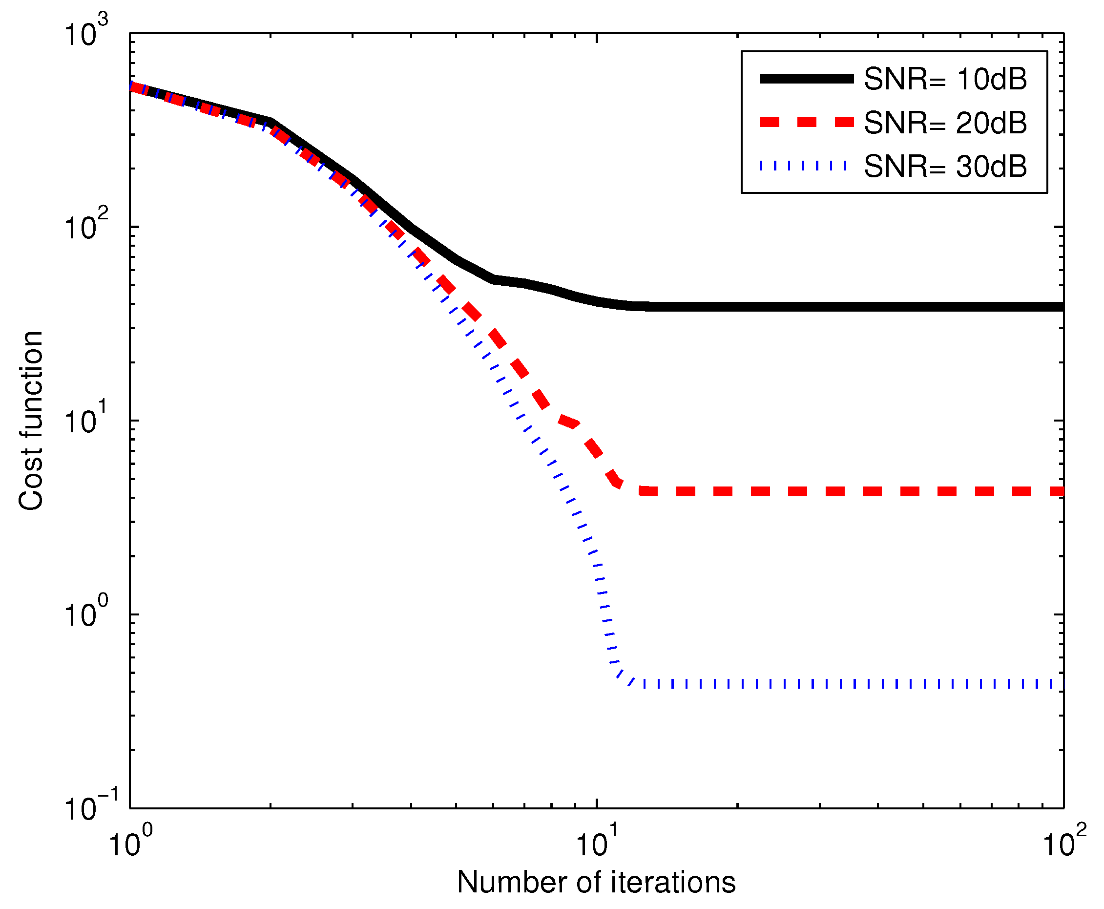
In the first example, we evaluate the convergence performance of the optimized LM algorithm, which is used in our semi-blind receiver. We assume the system design parameters $N=P=5$ and $R=3$. In Figure 2, the average value of the cost function is plotted versus the number of iterations, for three SNR values. We observe from Figure 2 that for each SNR value, the cost function decreases as the number of iterations increases until the algorithm converges. We can also see that for the same number of iterations, the cost function decreases as SNR increases. The proposed algorithm needs few iterations to converge. For instance, the optimized LM algorithm achieves convergence in about 10 iterations at the SNR of 20 dB.

In the second example, we evaluated the estimation performance of the proposed semi-blind receiver in terms of bit error rate (BER) and the NMSE of channel estimation. In particular, we compared the PARAFAC-based receiver with KRST (P-KRST) coding scheme in [8] and the training-based receiver with the space-time (TB-ST) coding scheme. For the TB-ST scheme, the symbol matrix is composed of two parts as in [9], i.e., the training symbol matrix and the unknown data symbol matrix. $N_{tr}$ denotes the length of the channel training sequence in the TB-ST receiver.

The transmission rates for the proposed coding scheme and the KRST coding scheme are $\frac{RN}{PN}=\frac{R}{P}$ and $\frac{M_{S}N}{PN}=\frac{M_S}{P}$ (data symbols per symbol period), respectively. However, the KRST coding scheme needs to know the first column of signal matrix $\mathbf{S}$ to eliminate the scaling ambiguity, while the proposed coding scheme only needs to know $s_{1,1}$ to eliminate the scaling ambiguity. Thus, the efficient transmission rates for the proposed coding scheme and the KRST coding scheme are $\frac{RN-1}{PN}$ and $\frac{M_S\left(N-1\right)}{PN}$, respectively. To ensure a fair comparison, the proposed coding scheme and the KRST coding scheme should keep the same efficient transmission rate, i.e., $N=\frac{M_S-1}{M_S-R}$. Thus, the system design parameters in this example are set equal to $M_S=4$, $P=7$, and $R=N=3$. For TB-ST coding scheme, we divide $P=P_{tr}+P_d$, where blocks $P_{tr}=2$ and $P_{tr}=5$ are used for channel training and data transmitting. Therefore, the length of the channel training sequence in the TB-ST receiver is $N_{tr}=P_{tr}N=6$.

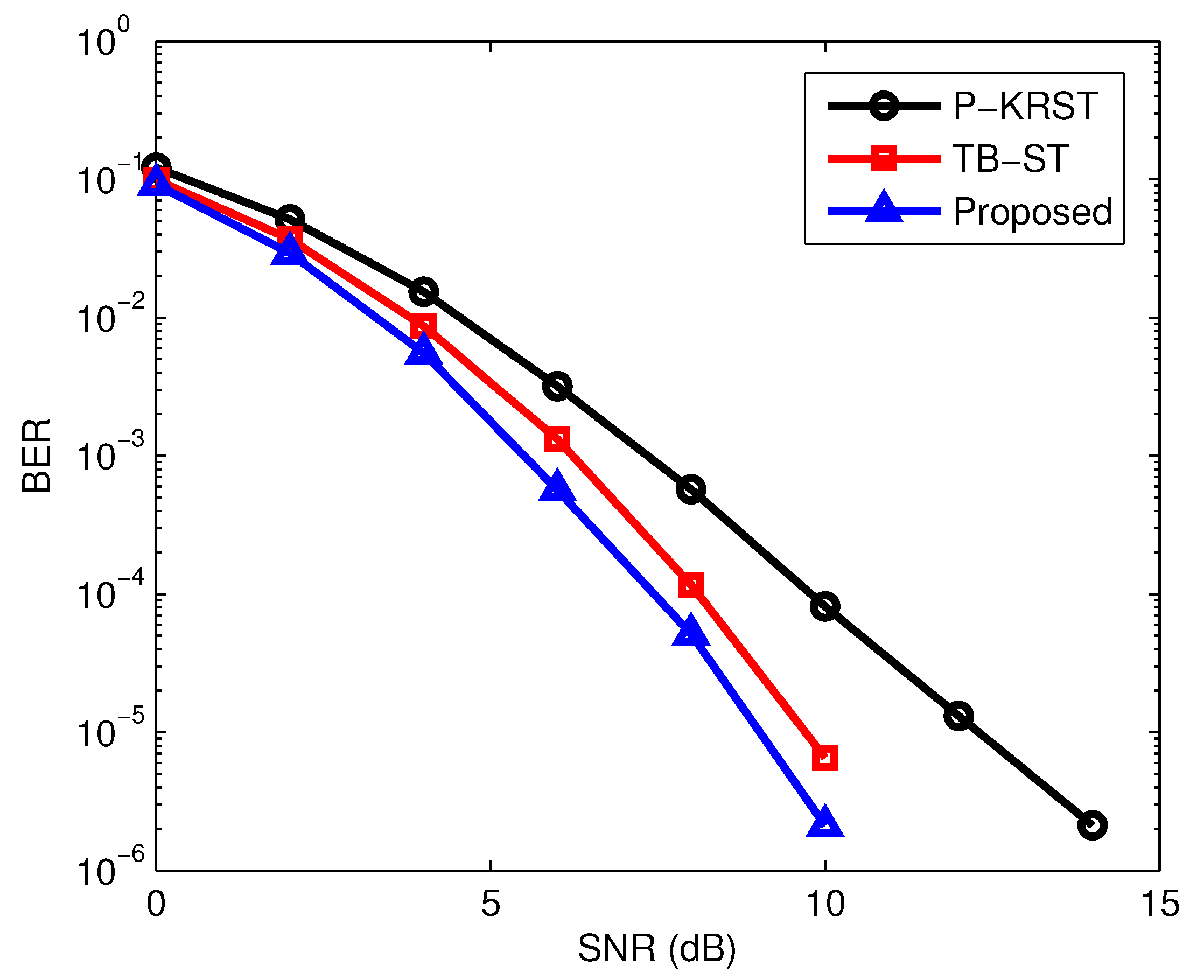
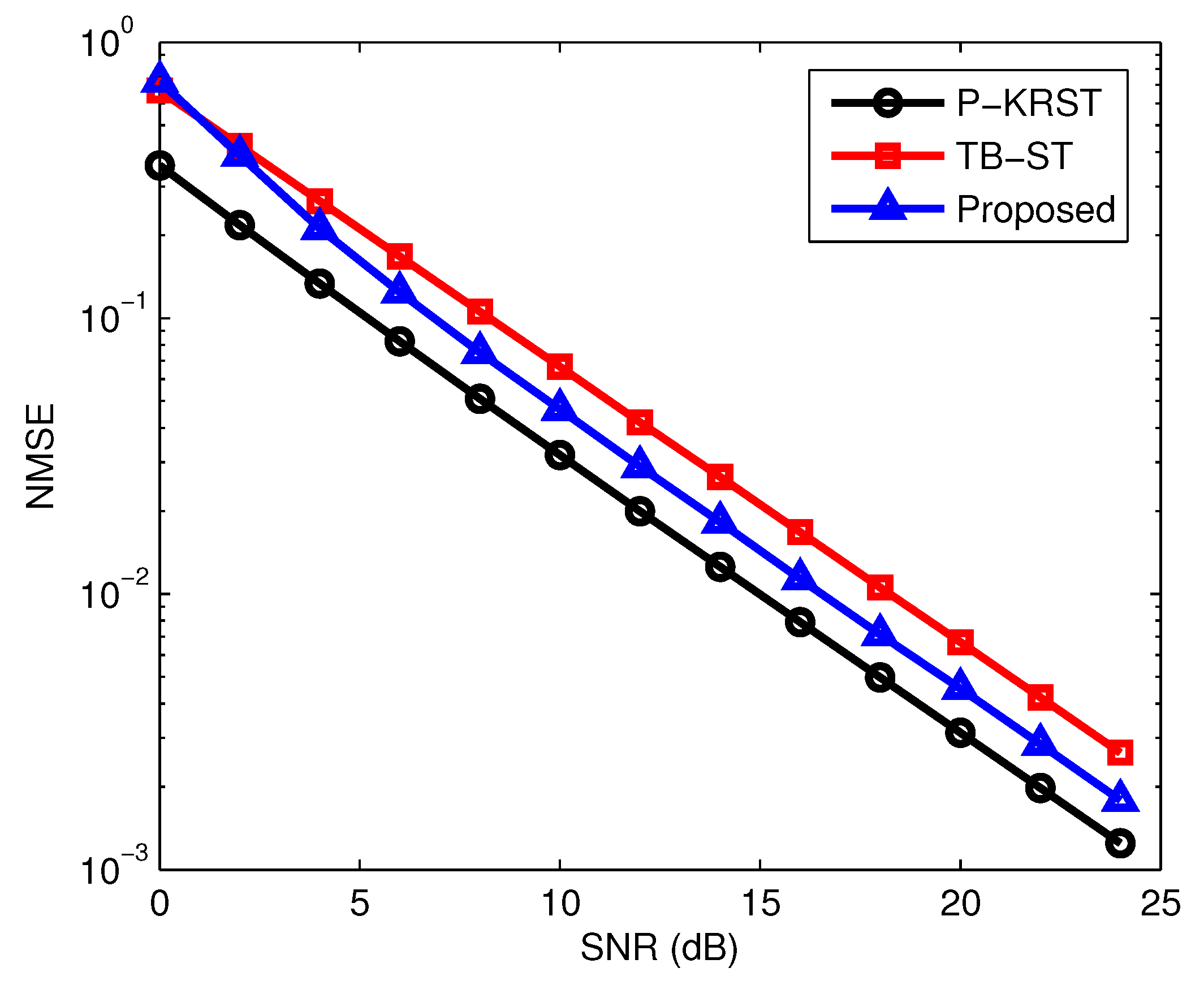
The BER performance of different receivers versus SNR is shown in Figure 3. It can be seen that the proposed semi-blind receiver outperforms the P-KRST and TB-ST receiver. The NMSE performance of the different receivers is demonstrated in Figure 4. It can be seen from Figure 4 that the P-KRST receiver has the best performance of channel estimation, and the proposed semi-blind receiver yields a smaller NMSE compared with the TB-ST receiver. From [8], the per-iteration complexity in the PARAFAC based receiver is $\mathcal{O}\left(M_S{M}_{D}PN\right)$. The complexity of the TB-ST scheme can be estimated as $\mathcal{O}\left(N_r{M}_S\left(M_D+N_r\right)+RP{M}_D\left(N+R\right)\right)$. The per-iteration complexity of the proposed O-LM algorithm is given at the end of Section 4. The TB-ST scheme has the least computational complexity due to the use of the channel training sequence. Due to the adoption of the simple KRST coding scheme, the PARAFAC based receiver has lower complexity than that of the proposed receiver. However, the TB-ST receiver requires a long channel training sequence, the PARAFAC-based receiver needs to know the first column or row of the signal matrix to eliminate the scaling ambiguity, but the proposed receiver only needs to know one symbol of the signal matrix.

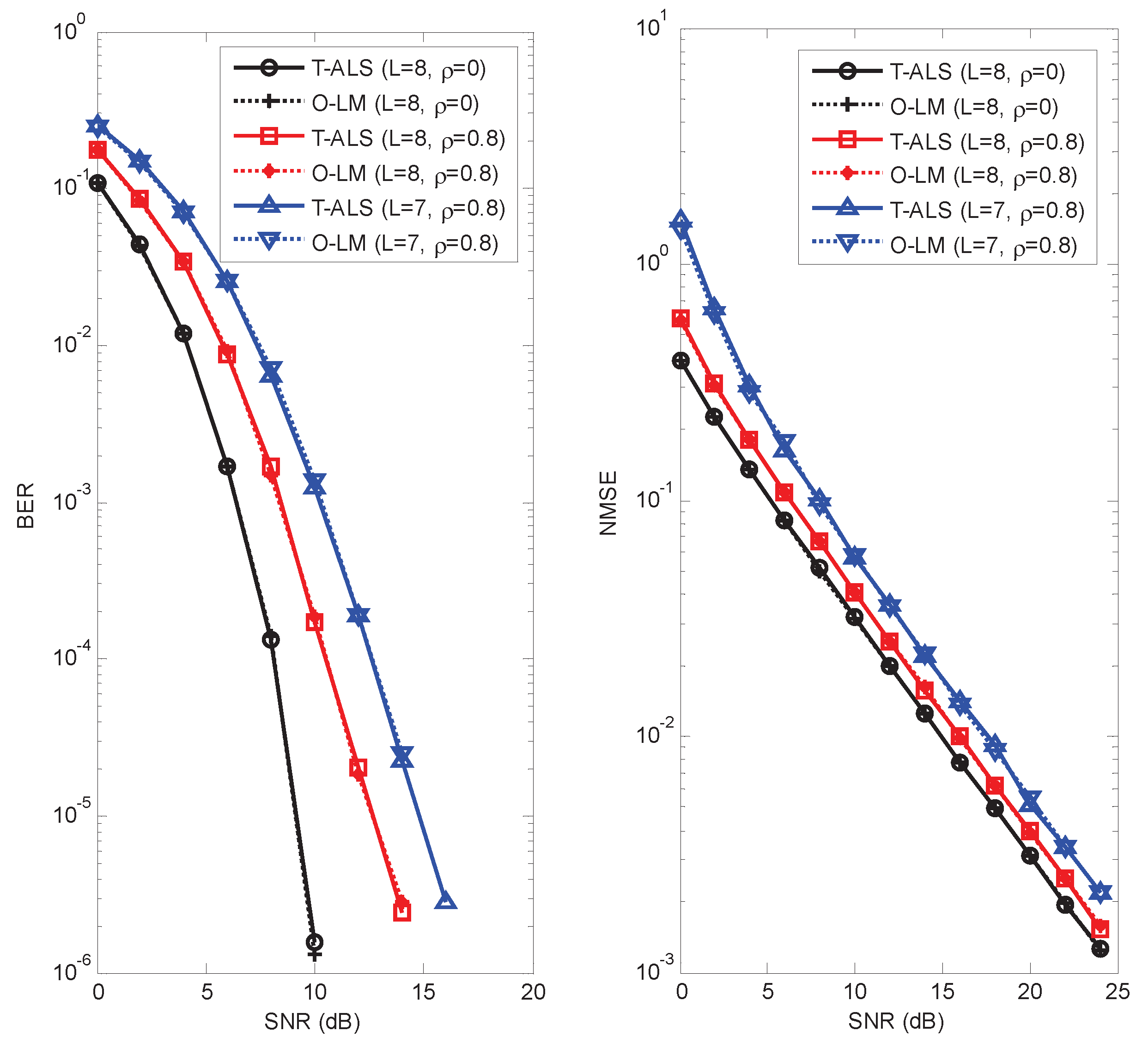
In the third example, we evaluated and compared the performance of the traditional ALS (T-ALS) and optimized LM (O-LM) algorithms. We assume the system design parameters $N=P=L$ and $R=5$. Correlated MIMO channel is considered in this example, and the channel matrix $\mathbf{H}$ is modeled as in [35], where $\rho$ denotes the normalized correlation coefficient with magnitude $\left|\rho \right|\le 1$. We consider $\rho =0$ (non-correlation) and $\rho =0.8$ (strong correlation), respectively. For each Monte Carlo run, the T-ALS algorithm is initialized with ten different random matrices as in [20,36]. The estimation performance is evaluated after selecting the best initialization, which is the one that results in the minimum value of ${\delta }^{\left(j\right)}$.

We observe from Figure 5 that the T-ALS and O-LM algorithms give a similar BER and NMSE performance, which means that these two algorithms converge to the same point. For the right subfigure of Figure 5, the NMSE of the T-ALS and O-LM algorithms is also shown in

Table 1. NMSE of the T-ALS and O-LM algorithms.

$\mathit{SNR}$ (dB)	0	2	4	6	8	10	12	14	16	18	20	22	24
$TALS$, $L=8$, $\rho =0$	0.3917	0.2265	0.1348	0.0822	0.0514	0.0318	0.0199	0.0124	0.0077	0.0049	0.0030	0.0019	0.0012
$O-LM$, $L=8$, $\rho =0$	0.3900	0.2253	0.1355	0.0814	0.0503	0.0317	0.0198	0.0124	0.0077	0.0049	0.0030	0.0019	0.0012
$TALS$, $L=8$, $\rho =0.8$	0.5920	0.3113	0.1803	0.1079	0.0666	0.0407	0.0251	0.0156	0.0100	0.0061	0.0039	0.0024	0.0015
$O-LM$, $L=8$, $\rho =0.8$	0.5777	0.3090	0.1814	0.1078	0.0664	0.0404	0.0251	0.0161	0.0098	0.0062	0.0039	0.0024	0.0015
$TALS$, $L=7$, $\rho =0.8$	1.5305	0.6519	0.3055	0.1623	0.1004	0.0570	0.0360	0.0221	0.0139	0.0091	0.0051	0.0034	0.0021
$O-LM$, $L=7$, $\rho =0.8$	1.4047	0.6228	0.2849	0.1770	0.0952	0.0580	0.0354	0.0221	0.0136	0.0087	0.0055	0.0034	0.0021

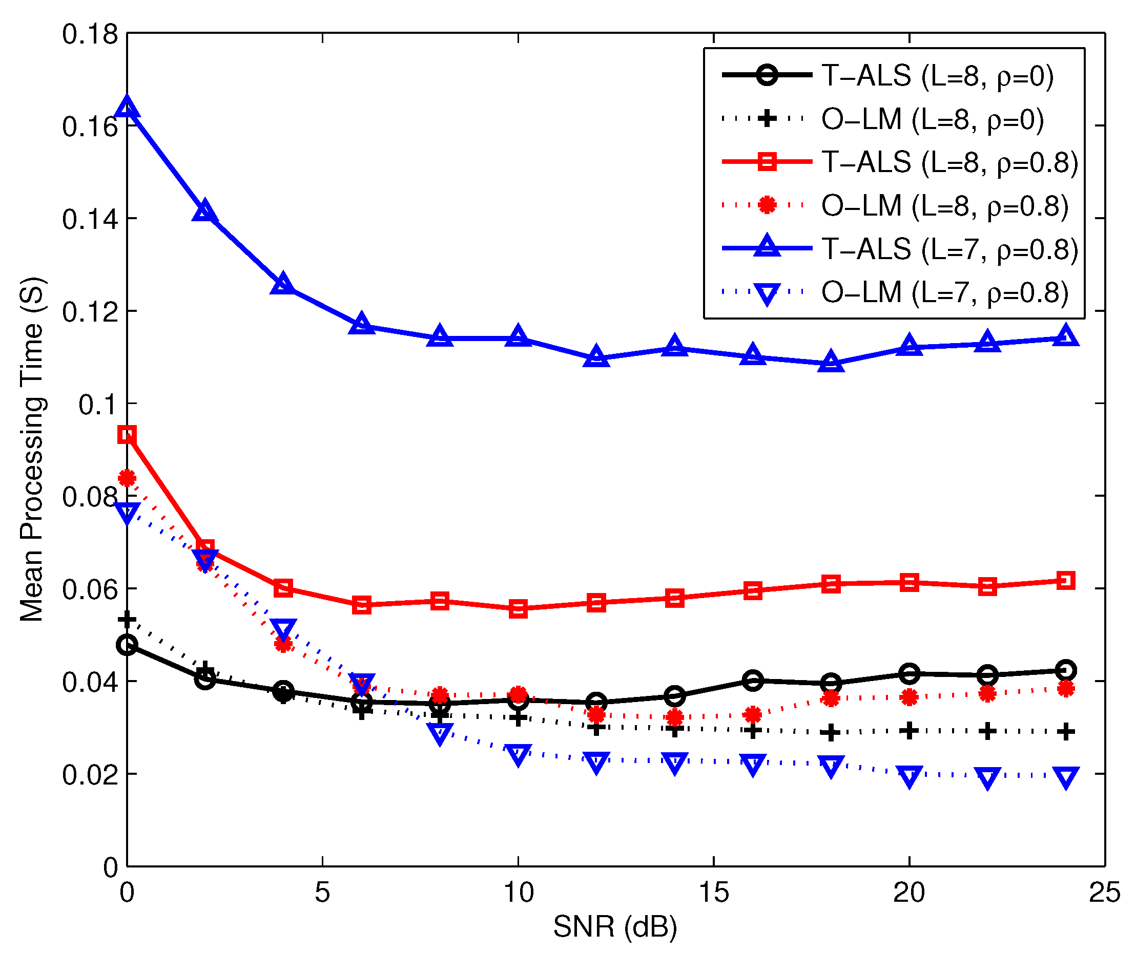
for the sake of comparison. We can also observe from Figure 5 that for these two algorithms, BER and NMSE performance degrade when the channel becomes strongly correlated. The overall complexities of the O-LM algorithm and the ALS algorithm depend on the per-iteration complexity and the number of iterations. The per-iteration complexity of the O-LM algorithm is higher than that of the T-ALS algorithm. However, because of the robustness of the O-LM algorithm, the O-LM algorithm needs fewer iterations compared with the T-ALS algorithm. Therefore, the proposed algorithm has lower complexity compared with the existing T-ALS algorithm. The mean processing times required in the T-ALS and O-LM algorithms are shown in Figure 6. We observe that the mean processing time required in the O-LM algorithm is shorter than that of the T-ALS algorithm, especially when the channel becomes strongly correlated. From Figure 6 we can also observe that the advantage of the O-LM algorithm is obvious as L decreases from 8 to 7 compared with the T-ALS algorithm.

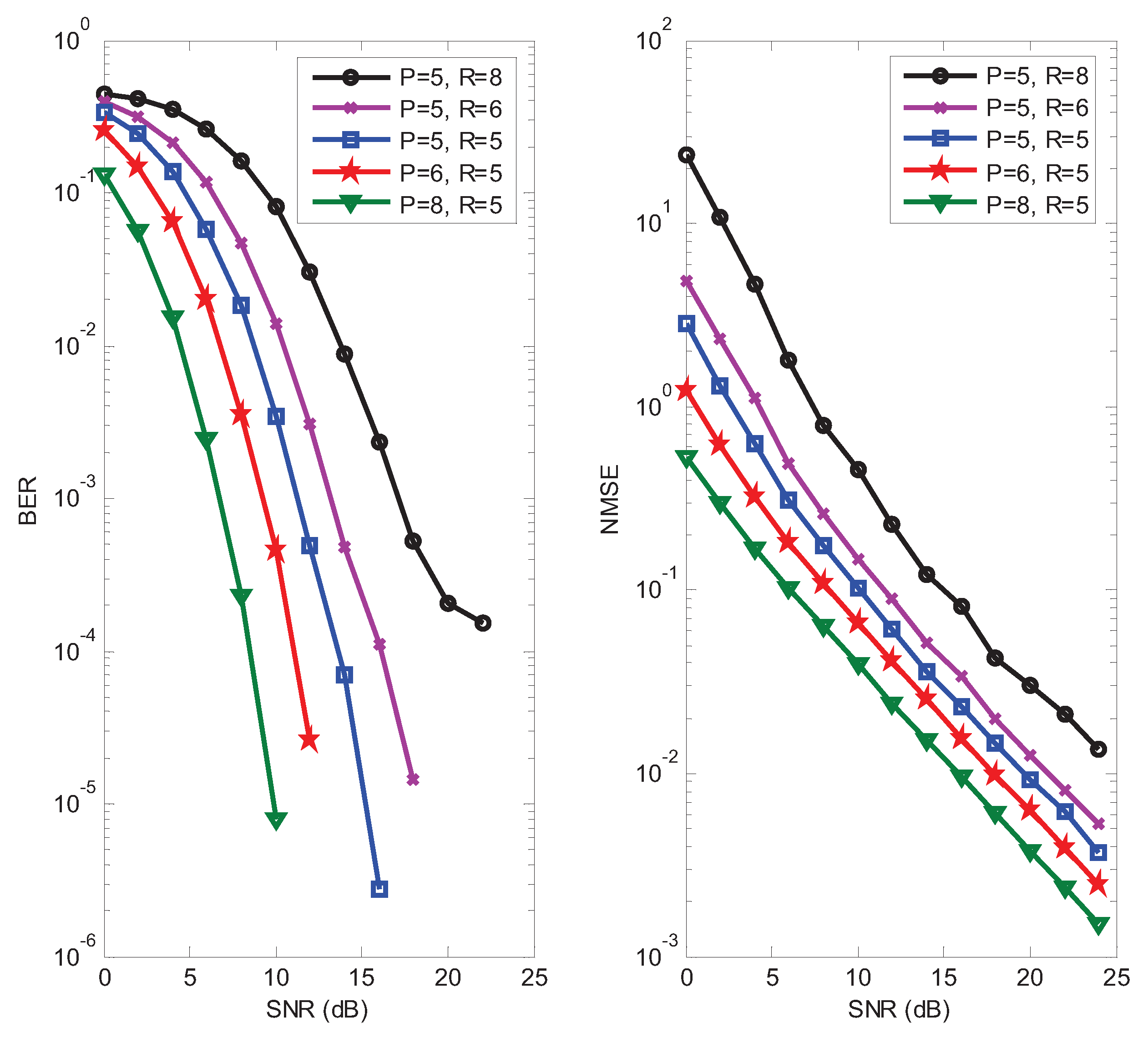
In the fourth example, the influence of design parameters $\left(P,R\right)$ for the proposed receiver is studied. In the left subfigure of Figure 7, it can be seen that the BER decreases when P increases, which expounds the performance gain brought by the time diversity. It can also be seen from this subfigure that the BER increases as the number of data streams R increases. The impact of design parameters $\left(P,R\right)$ on the NMSE performance is shown in the right subfigure of Figure 7. As expected, we can observe that the NMSE decreases linearly as a function of P, and increases as R increases. Hence, appropriate values for the design parameters P and R can be selected according to requirements of the system performance and transmission rate.

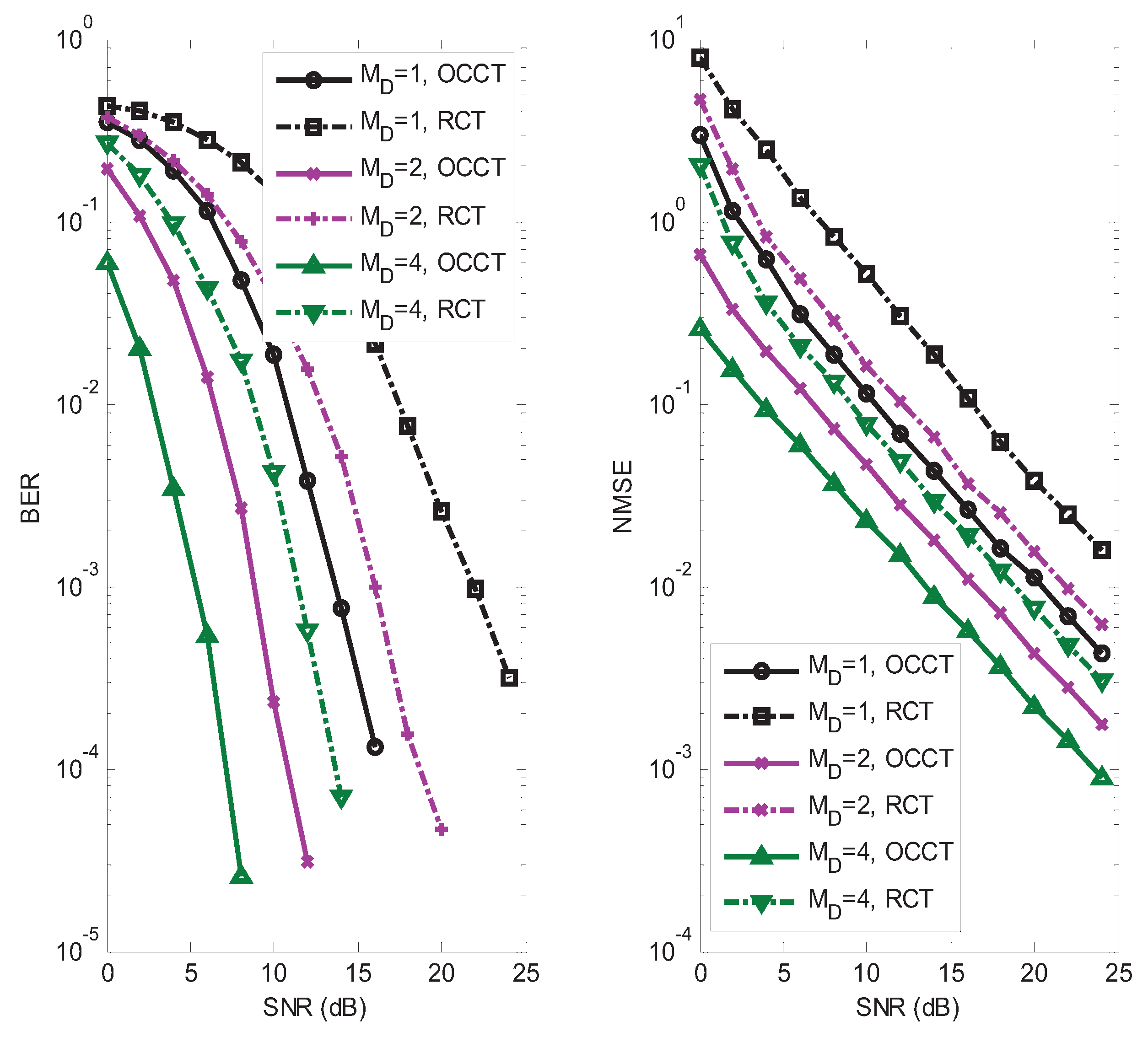
In the fifth example, we assume $M_S=3$, $R=4$, and $N=P=8$ for our semi-blind receiver. The influence of the receive antenna was analyzed. We also compared the performance of our chosen coding tensor (OCCT) $\underline{\mathbf{B}}$ with the random coding tensor (RCT) whose entries are circularly-symmetric Gaussian random variables. In Figure 8, it can be seen that both the BER and NMSE decrease when $M_D$ increases, which expounds the performance gain brought by the receive diversity. We also observed from Figure 8 that OCCT has a better performance than RCT. Although OCCT is suboptimal, this choice has good symbol and channel identifiability properties, which is advantageous from a receiver design viewpoint.

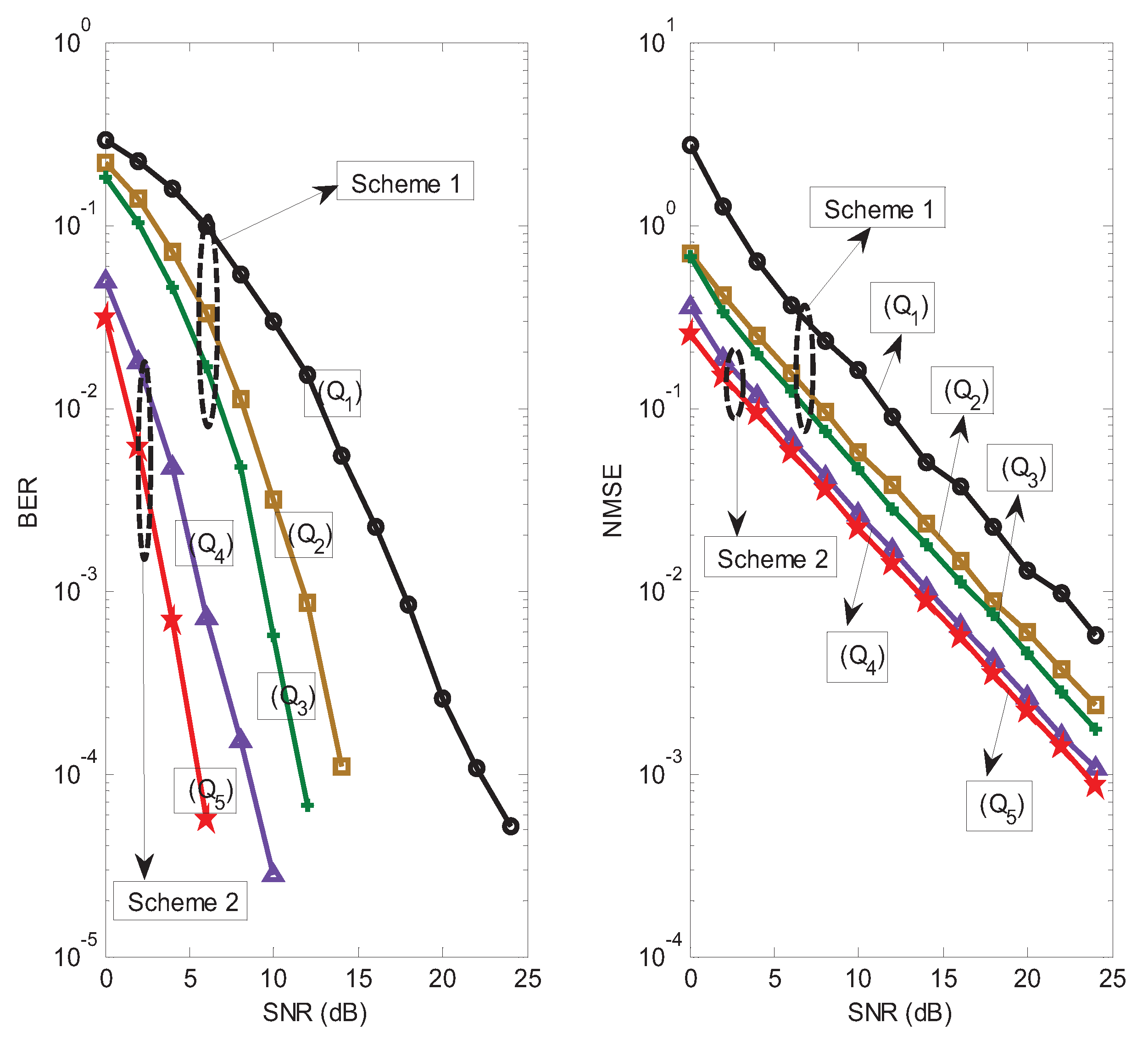
In the sixth example, we studied the estimation performance of two different transmission schemes for our semi-blind receiver. The default values of the system parameters were set to $M_D=5$ and $N=6$. In scheme 1, we assume $M_S=2$, $R=5$, and $P=6$. Three different antenna-to-slot allocation matrices are given as follows:

$${\mathbf{Q}}_1=\left[\begin{array}{c}10\hfill \\ 01\hfill \\ 10\hfill \\ 10\hfill \\ 01\hfill \\ 10\hfill \end{array}\right],{\mathbf{Q}}_2=\left[\begin{array}{c}01\hfill \\ 11\hfill \\ 10\hfill \\ 01\hfill \\ 11\hfill \\ 10\hfill \end{array}\right],{\mathbf{Q}}_3=\left[\begin{array}{c}11\hfill \\ 01\hfill \\ 11\hfill \\ 10\hfill \\ 11\hfill \\ 11\hfill \end{array}\right]$$

In scheme 2, we assume $M_S=3$, $R=3$, and $P=7$. Three different antenna-to-slot allocation matrixes are given as follows:

$${\mathbf{Q}}_4=\left[\begin{array}{c}100\hfill \\ 100\hfill \\ 101\hfill \\ 100\hfill \\ 010\hfill \\ 010\hfill \\ 101\hfill \end{array}\right],{\mathbf{Q}}_5=\left[\begin{array}{c}101\hfill \\ 110\hfill \\ 111\hfill \\ 110\hfill \\ 111\hfill \\ 010\hfill \\ 111\hfill \end{array}\right]$$

The BER and NMSE performance of the proposed receiver for different schemes is shown in Figure 9. For scheme 1, the proposed receiver with ${\mathbf{Q}}_2$ has a better BER and NMSE performance than that of the proposed receiver with ${\mathbf{Q}}_1$. The reason is that the allocation matrix ${\mathbf{Q}}_2$ provides a higher transmit spatial diversity gain than the allocation matrix ${\mathbf{Q}}_1$. For the same reason, the allocation matrix ${\mathbf{Q}}_3$ outperforms ${\mathbf{Q}}_2$, and the allocation matrix ${\mathbf{Q}}_5$ outperforms ${\mathbf{Q}}_4$. We also observe in Figure 9 that scheme 2 has a better BER and NMSE performance than scheme 1. The reason is that scheme 2 can provide a higher coding diversity than scheme 1. It is worth noting that scheme 1 has higher spectral efficiency compared with scheme 2. The transmission rates for scheme 1 and scheme 2 are about 5/6 and 3/7 (data symbols per symbol period), respectively. In summary, a desired tradeoff between estimation performance and transmission rate can be obtained by designing a suitable scheme.

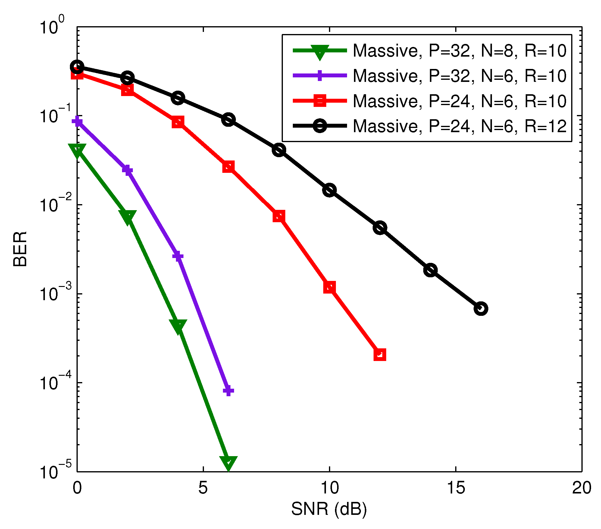
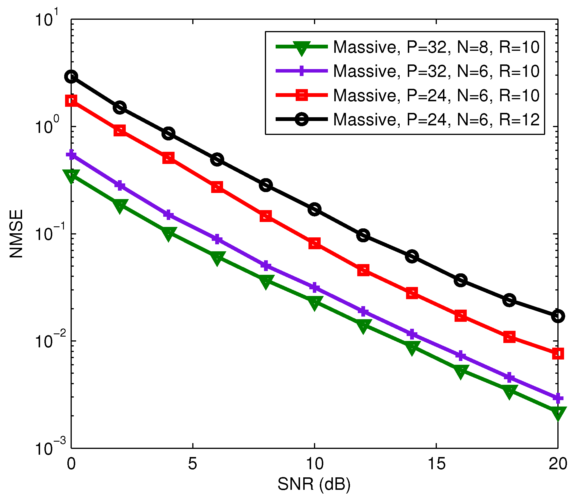
In final example, the multi-user massive MIMO system with a fully-connected hybrid precoding architecture was considered, where $M_S=48$, $M\times M_D=6\times 6$, and $L_m=2$ for all $m=1,\dots ,M$. The carrier frequency of this system is set as 28 GHz [37], and $d=\lambda /\phantom{\lambda 2}2$. We assume that AoAs/AoDs are uniformly distributed in $\left[0,2\pi \right]$. For the considering multi-user massive MIMO system, we also evaluate the estimation performance of the proposed receiver in terms of BER and NMSE of channel estimation. It can be seen from Figure 10 and Figure 11 that the BER and NMSE of the proposed semi-blind receiver decrease as P and N increase, and increase as R increases. The increase of P will reduce the transmission rate, but the increase or decrease of N has no effect on the transmission rate. That means that we can improve the estimation performance of the proposed semi-blind receiver by increasing N if the channel is constant over a long time interval before changing to another realization. We also observed from Figure 10 and Figure 11 that the proposed semi-blind receiver still has a good performance for joint symbol and channel estimation even in a shorter length of code and information symbol, and a larger number of data streams, i.e., $P=24$, $N=6$, and $R=12$.

7. Conclusions

We have developed a robust semi-blind receiver combined with the Tucker-2 model in multiple-antenna systems. The proposed receiver could jointly estimate the information symbol and channel parameters. Compared with existing semi-blind receivers, the proposed one gave better estimation performance, and had a higher spectral efficiency Moreover, the proposed semi-blind receiver was also applicable to multi-user massive MIMO systems. Perspectives of this work include an extension to relay-assisted massive MIMO systems by applying the antenna allocation matrix at the relays. Since both the source-relay and the relay-destination channel matrices have low-rank property, new identifiability conditions and efficient fitting algorithms will be deduced and developed, respectively. Another perspective considers extending the proposed robust semi-blind receiver into mmwave MIMO systems for joint channel parameter estimation, which includes AOAs, fading coefficients and time delays [38,39].