Regularized Auto-Encoder-Based Separation of Defects from Backgrounds for Inspecting Display Devices


Abstract
:1. Introduction
2. Related Works
2.1. Low-Rank-Approximation-Based Method
2.2. Auto-Encoder Based Segmentation
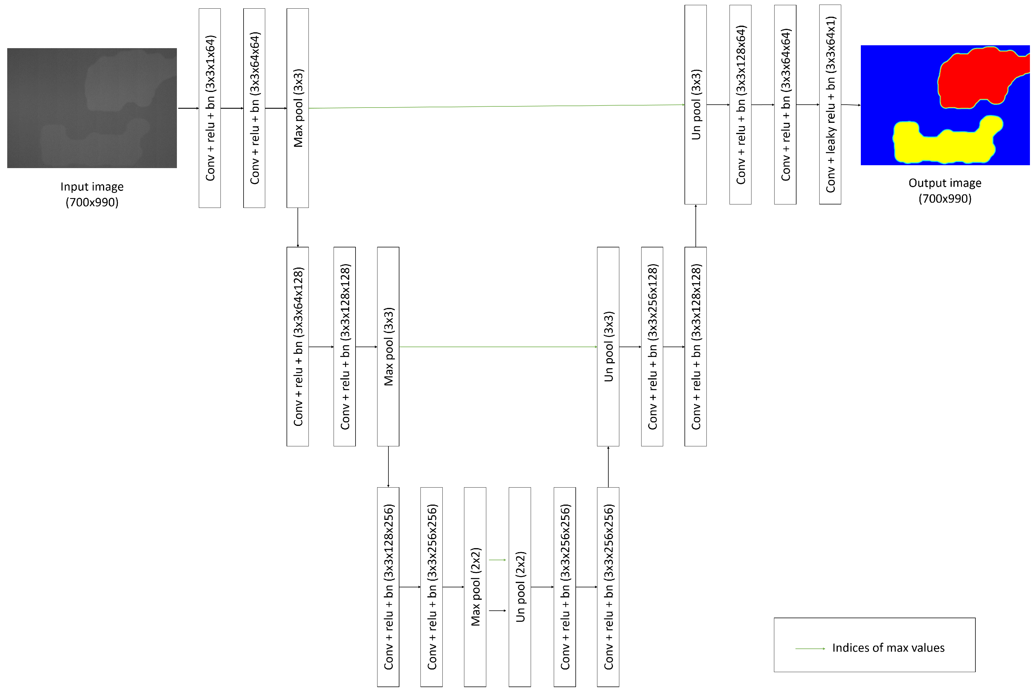
3. Proposed Method
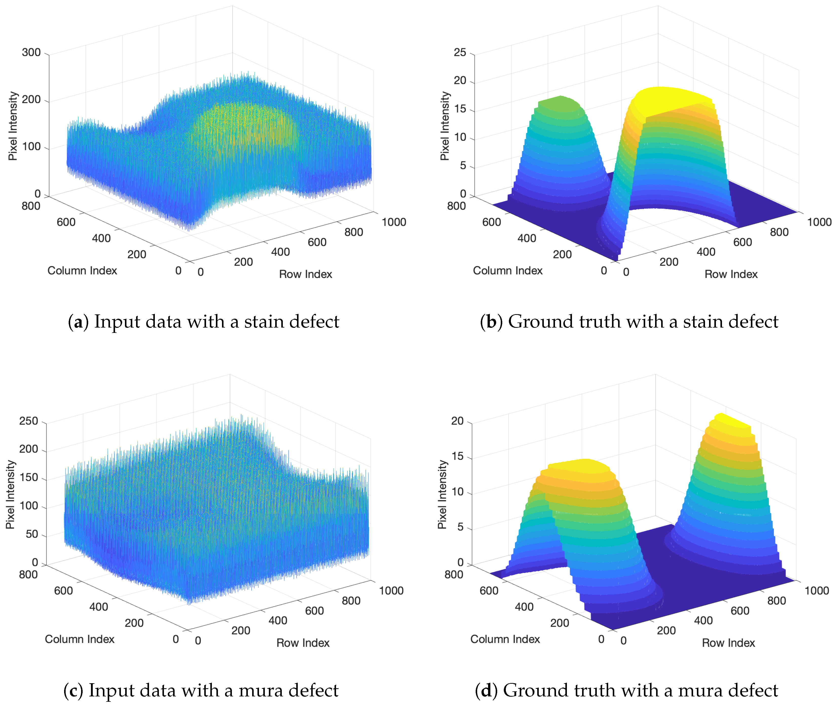
3.1. Problem Formulation
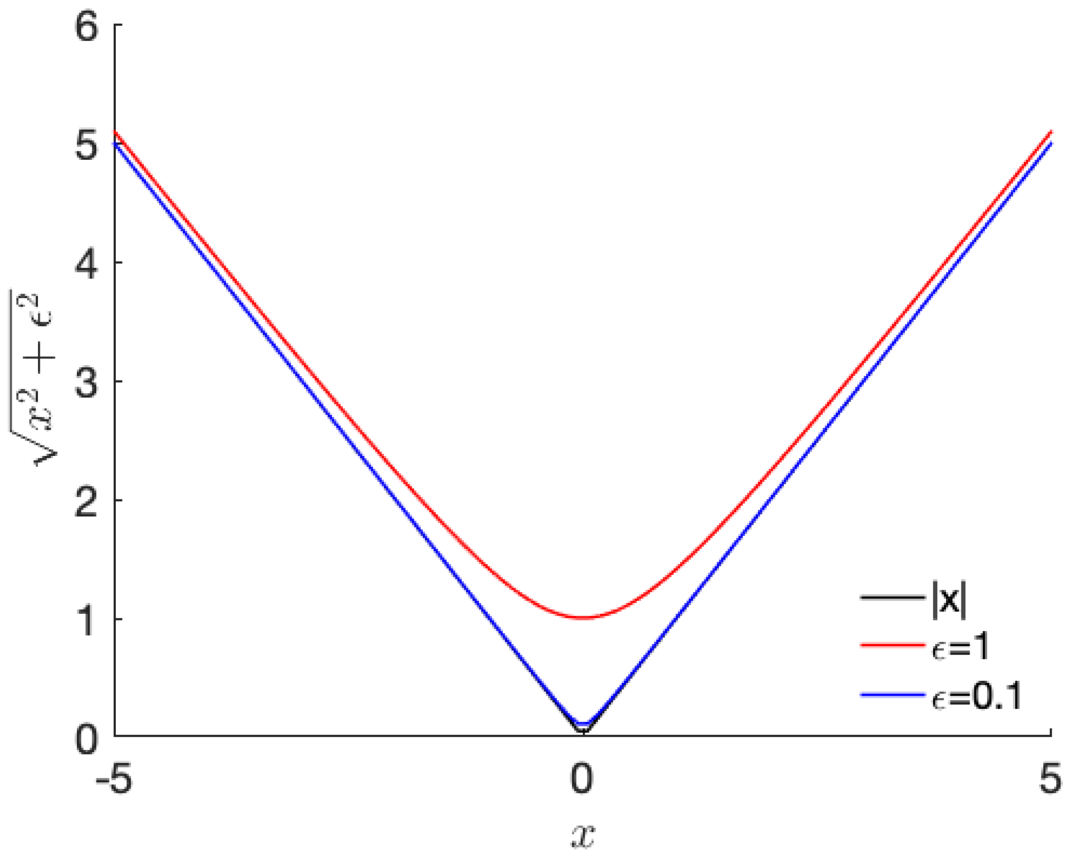
3.2. Separating Defects Using Auto-Encoder Based Regression with Regularization
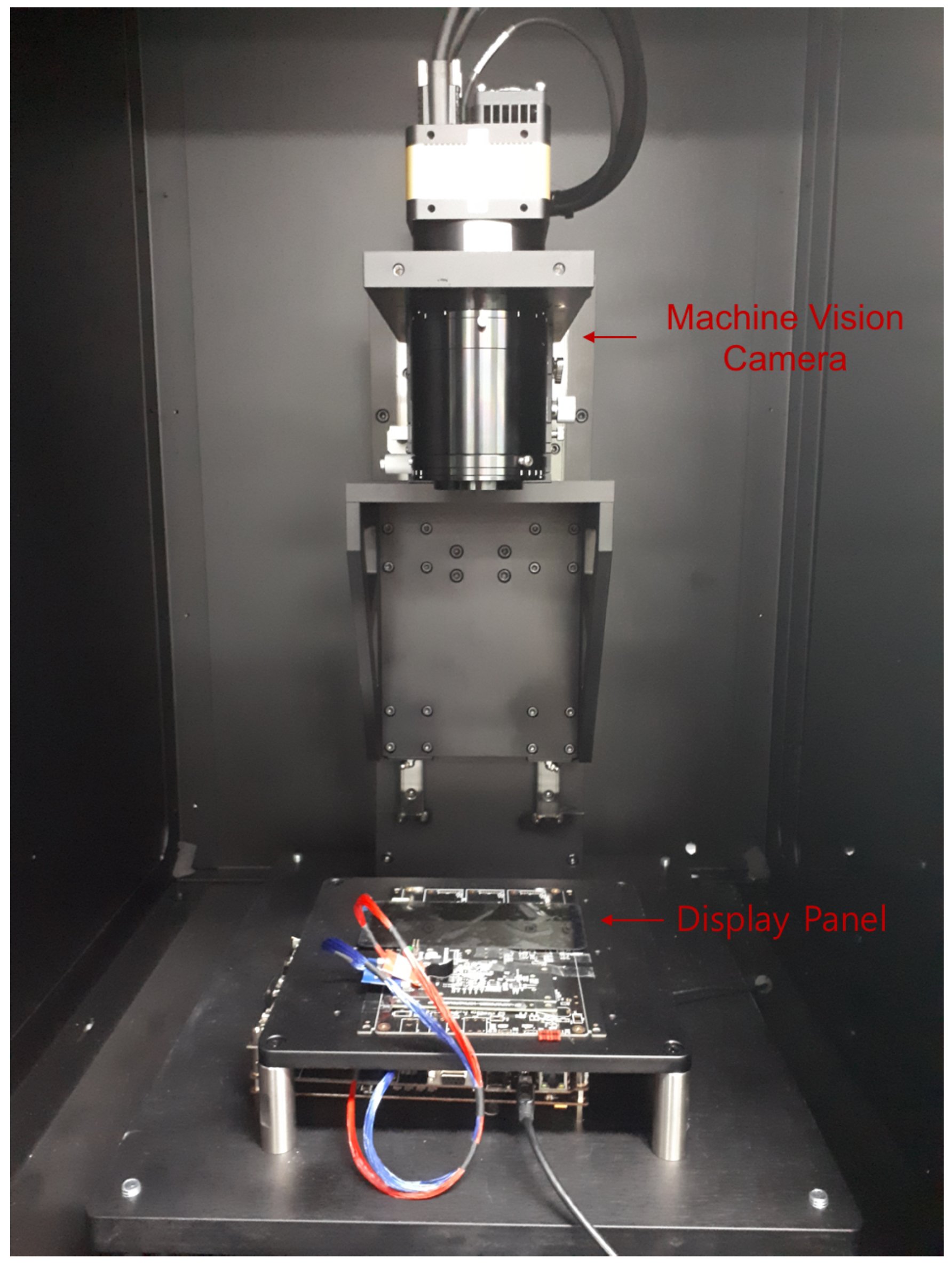
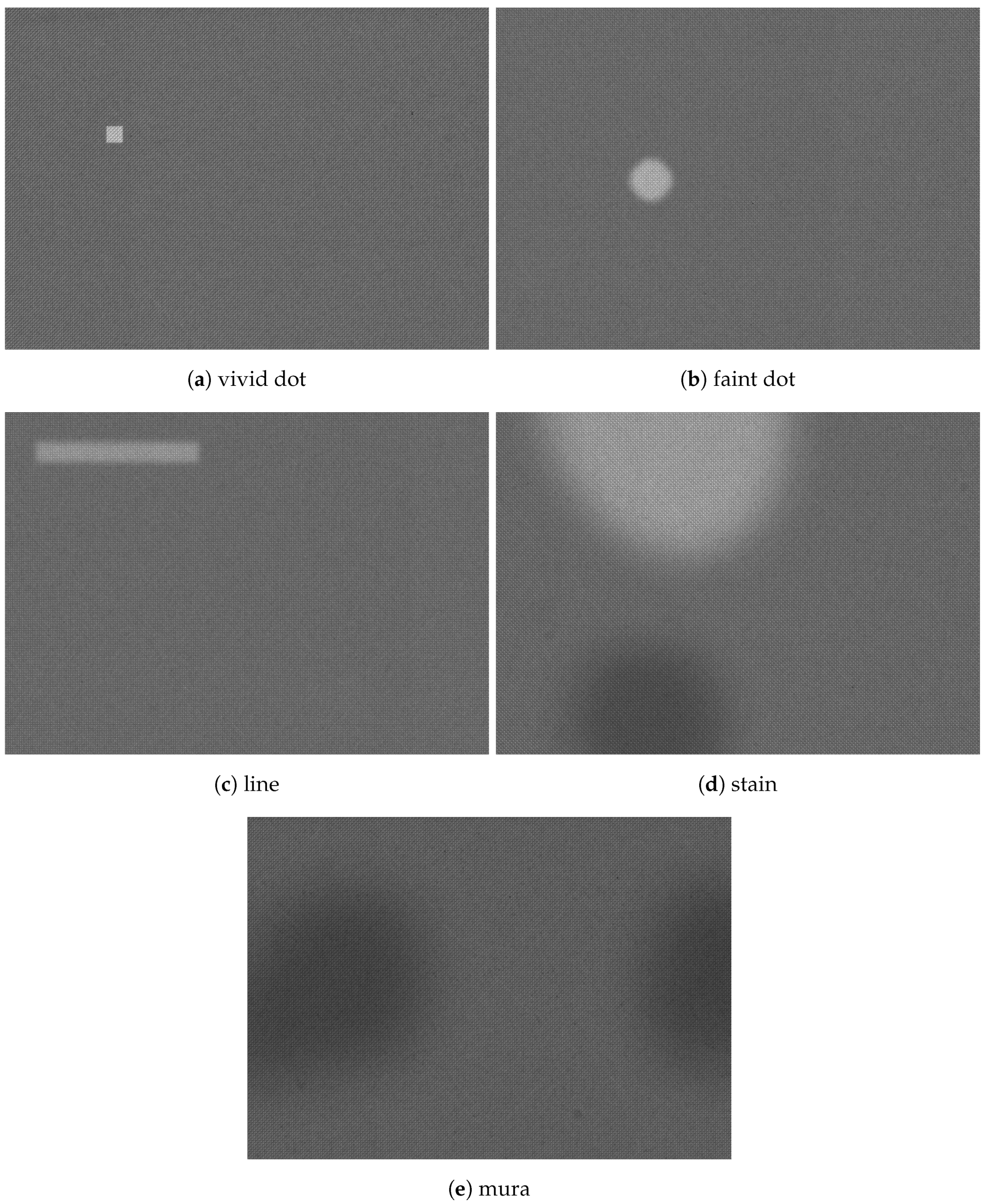
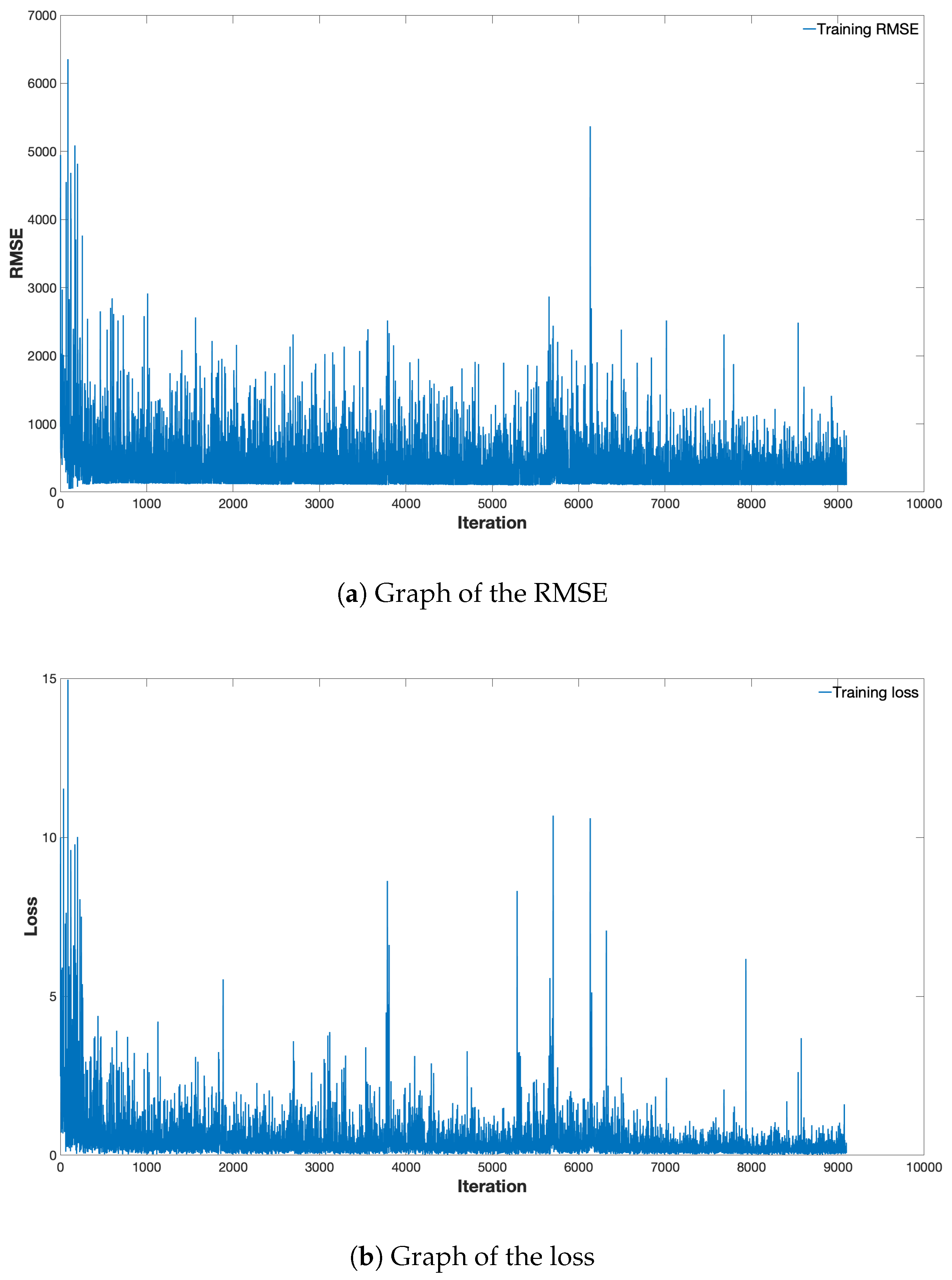
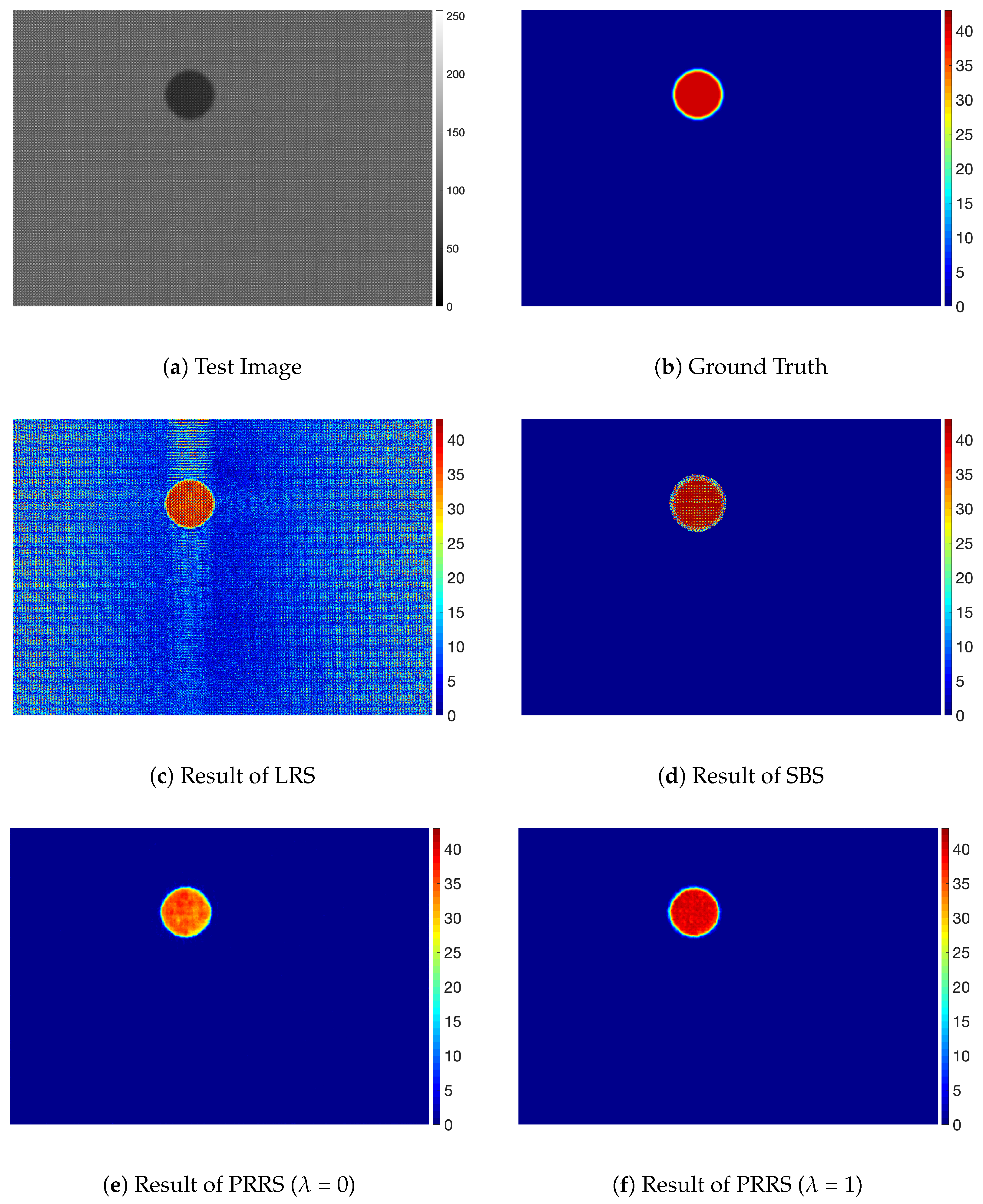
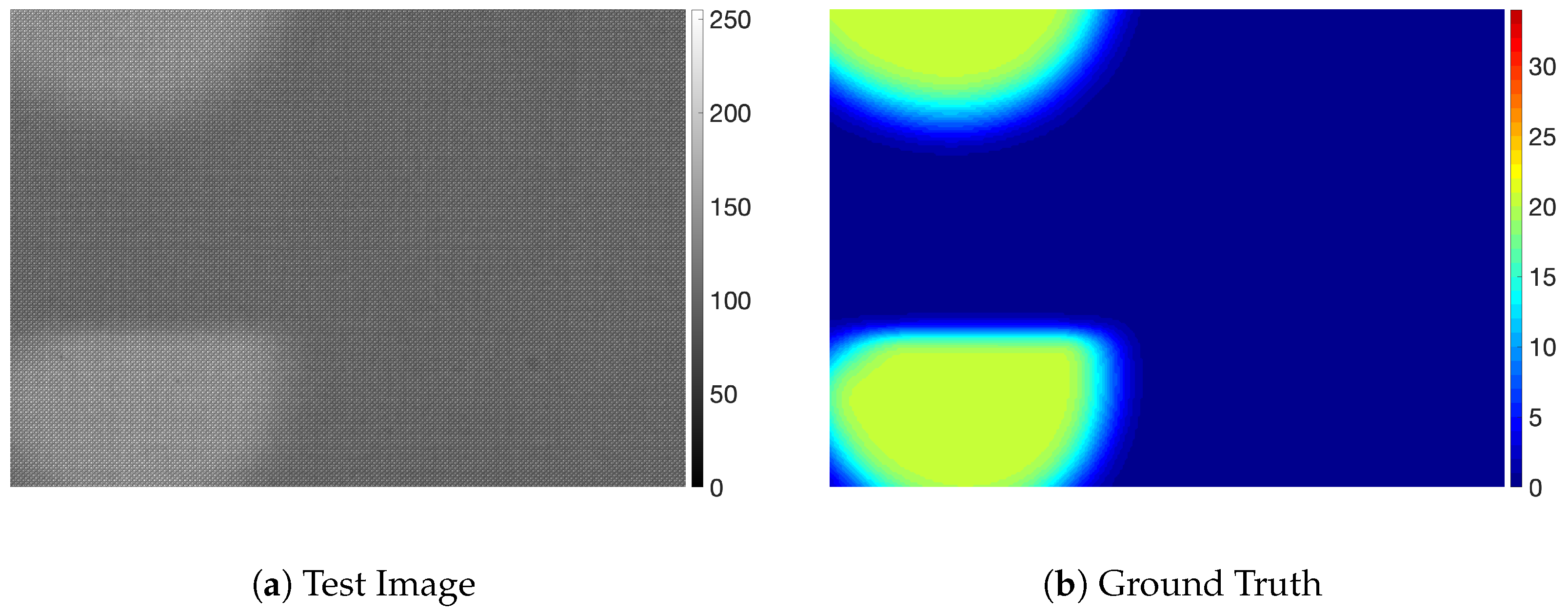
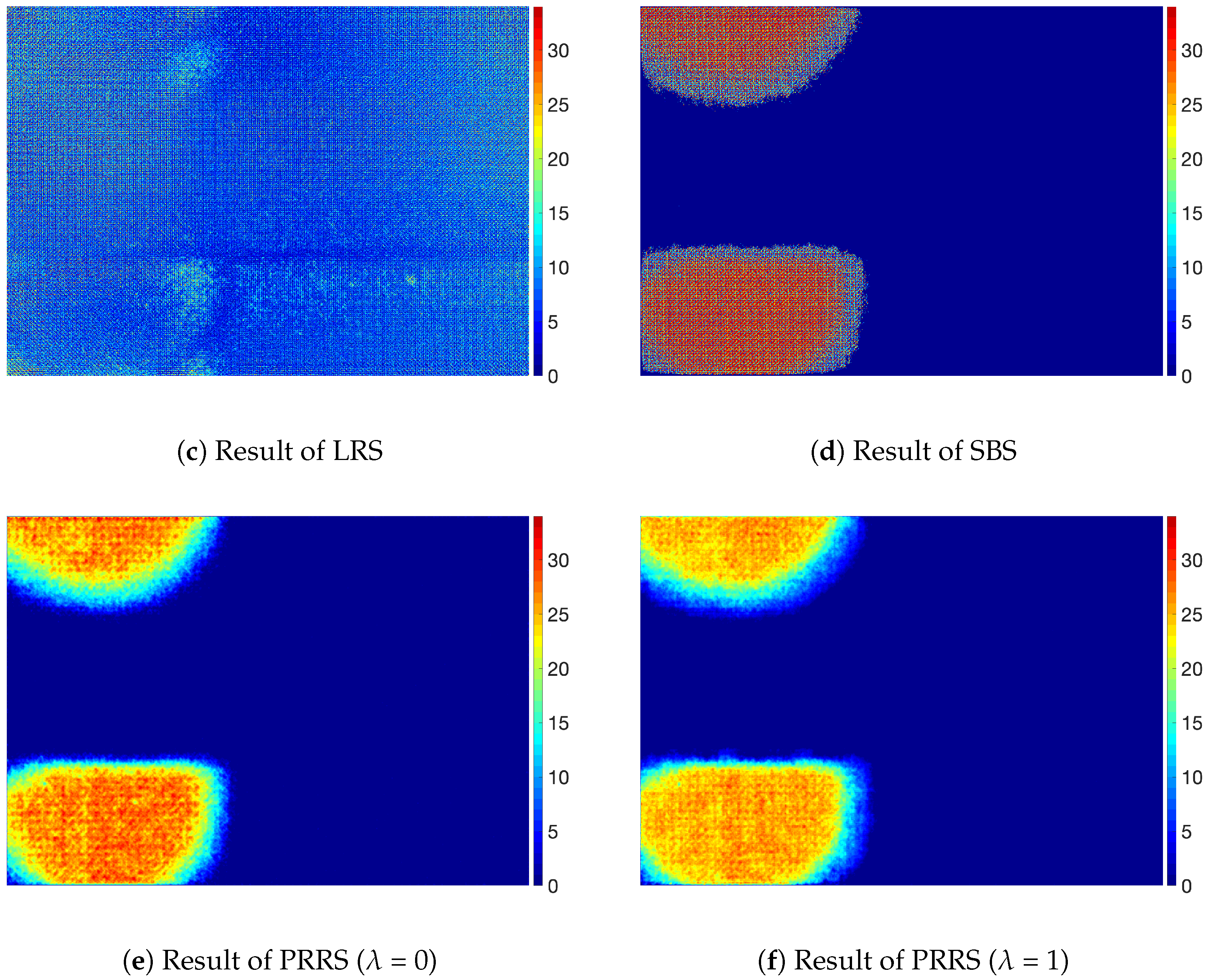
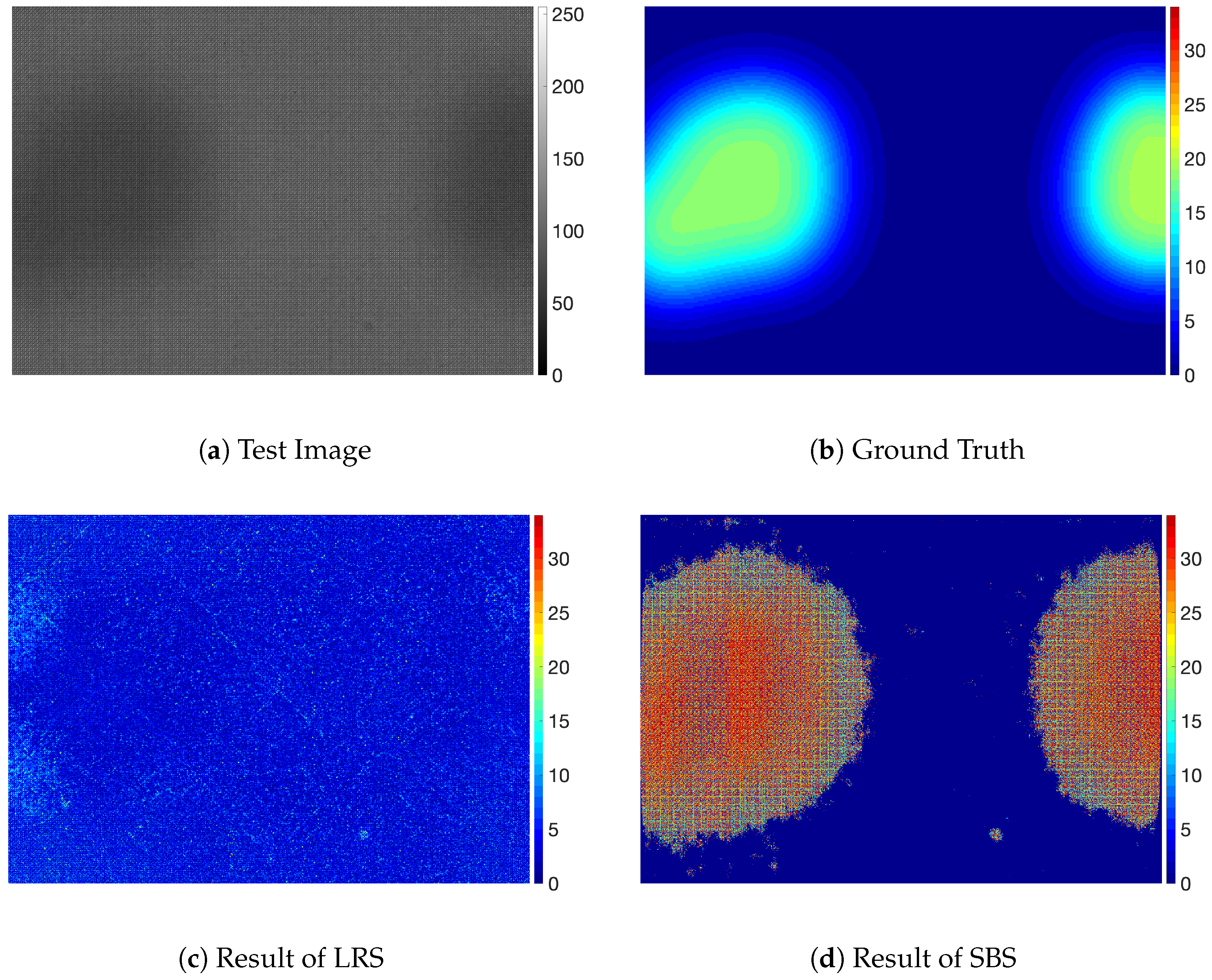
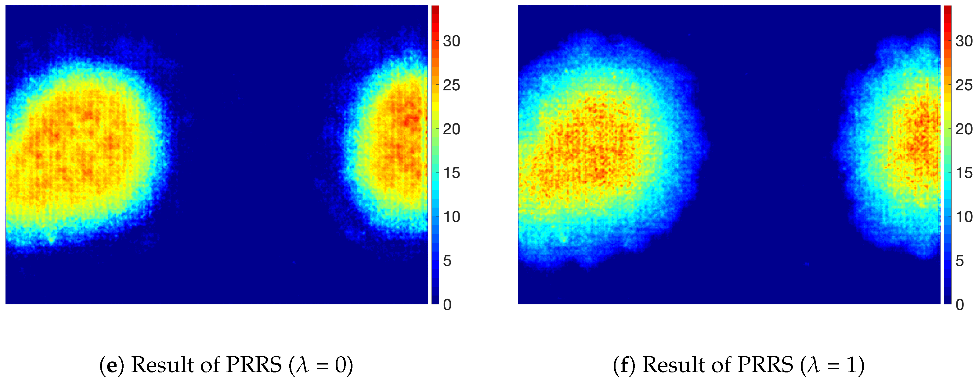
4. Results
5. Conclusions
Author Contributions
Funding
Acknowledgments
Conflicts of Interest
References
- Baek, S.I.; Kim, W.S.; Koo, T.M.; Choi, I.; Park, K.H. Inspection of defect on LCD panel using polynomial approximation. In Proceedings of the 2004 IEEE Region 10 Conference (TENCON 2004), Chiang Mai, Thailand, 24 November 2004; pp. 235–238. [Google Scholar]
- Bi, X.; Xu, X.; Shen, J. An automatic detection method of Mura defects for liquid crystal display using real Gabor filters. In Proceedings of the 2015 8th International Congress on Image and Signal Processing (CISP), Shenyang, China, 14–16 October 2015; pp. 871–875. [Google Scholar]
- Cen, Y.G.; Zhao, R.Z.; Cen, L.H.; Cui, L.; Miao, Z.; Wei, Z. Defect inspection for TFT-LCD images based on the low-rank matrix reconstruction. Neurocomputing 2015, 149, 1206–1215. [Google Scholar] [CrossRef]
- Jamleh, H.; Li, T.Y.; Wang, S.Z.; Chen, C.W.; Kuo, C.C.; Wang, K.S.; Chen, C.C.P. 50.2: Mura detection automation in LCD panels by thresholding fused normalized gradient and second derivative responses. In SID Symposium Digest of Technical Papers; Blackwell Publishing Ltd.: Oxford, UK, 2010; Volume 41, pp. 746–749. [Google Scholar]
- Bi, X.; Zhuang, C.; Ding, H. A new mura defect inspection way for TFT-LCD using level set method. IEEE Signal Process. Lett. 2009, 16, 311–314. [Google Scholar]
- Chen, L.C.; Kuo, C.C. Automatic TFT-LCD mura defect inspection using discrete cosine transform-based background filtering and ‘just noticeable difference’quantification strategies. Meas. Sci. Technol. 2007, 19, 015507. [Google Scholar] [CrossRef]
- Wang, Z.; Gao, J.; Jian, C.; Cen, Y.; Chen, X. OLED Defect Inspection System Development through Independent Component Analysis. TELKOMNIKA Indones. J. Electr. Eng. 2012, 10, 2309–2319. [Google Scholar] [CrossRef]
- Lu, C.J.; Tsai, D.M. Automatic defect inspection for LCDs using singular value decomposition. Int. J. Adv. Manuf. Technol. 2004, 25, 53–61. [Google Scholar] [CrossRef]
- Lu, C.J.; Tsai, D.M. Defect inspection of patterned thin film transistor-liquid crystal display panels using a fast sub-image-based singular value decomposition. Int. J. Prod. Res. 2007, 42, 4331–4351. [Google Scholar] [CrossRef]
- Perng, D.B.; Chen, S.H. Directional textures auto-inspection using discrete cosine transform. Int. J. Prod. Res. 2011, 49, 7171–7187. [Google Scholar] [CrossRef]
- Chen, S.H.; Perng, D.B. Directional textures auto-inspection using principal component analysis. Int. J. Adv. Manuf. Technol. 2011, 55, 1099–1110. [Google Scholar] [CrossRef]
- Gan, Y.; Zhao, Q. An effective defect inspection method for LCD using active contour model. IEEE Trans. Instrum. Meas. 2013, 62, 2438–2445. [Google Scholar] [CrossRef]
- Tseng, D.C.; Lee, Y.C.; Shie, C.E. LCD mura detection with multi-image accumulation and multi-resolution background subtraction. Int. J. Innov. Comput. Inf. Control 2012, 8, 4837–4850. [Google Scholar]
- Badrinarayanan, V.; Kendall, A.; Cipolla, R. SegNet: A Deep Convolutional Encoder-Decoder Architecture for Image Segmentation. IEEE Trans. Pattern Anal. Mach. Intell. 2017, 39, 2481–2495. [Google Scholar] [CrossRef] [PubMed]
- Ronneberger, O.; Fischer, P.; Brox, T. U-net: Convolutional networks for biomedical image segmentation. In Proceedings of the International Conference on Medical Image Computing and Computer-Assisted Intervention, Munich, Germany, 5–9 October 2015; pp. 234–241. [Google Scholar]
- Kumar, P.; Nagar, P.; Arora, C.; Gupta, A. U-Segnet: Fully Convolutional Neural Network Based Automated Brain Tissue Segmentation Tool. In Proceedings of the 2018 25th IEEE International Conference on Image Processing (ICIP), Athens, Greece, 7–10 October 2018; pp. 3503–3507. [Google Scholar]
- Chen, Q.; Montesinos, P.; Sen Sun, Q.; Heng, P.A.; Xia, D.S. Adaptive total variation denoising based on difference curvature. Image Vis. Comput. 2010, 28, 298–306. [Google Scholar] [CrossRef]
- Block, K.T.; Uecker, M.; Frahm, J. Undersampled radial MRI with multiple coils. Iterative image reconstruction using a total variation constraint. Magn. Reson. Med. 2007, 57, 1086–1098. [Google Scholar] [CrossRef] [PubMed]
- Anderson, D.; Sweeney, J.; Williams, T. Statistics for Business and Economics. South-Western; Thomson Learning Publishing Company: Cincinnati, OH, USA, 2002. [Google Scholar]
- Jenkins, M.D.; Carr, T.A.; Iglesias, M.I.; Buggy, T.; Morison, G. A Deep Convolutional Neural Network for Semantic Pixel-Wise Segmentation of Road and Pavement Surface Cracks. In Proceedings of the 2018 26th European Signal Processing Conference (EUSIPCO), Rome, Italy, 3–7 September 2018; pp. 2120–2124. [Google Scholar]
- Naresh, Y.G.; Little, S.; O’Connor, N.E. A Residual Encoder-Decoder Network for Semantic Segmentation in Autonomous Driving Scenarios. In Proceedings of the 2018 26th European Signal Processing Conference (EUSIPCO), Rome, Italy, 3–7 September 2018. [Google Scholar]
- Kendall, A.; Badrinarayanan, V.; Cipolla, R. Bayesian segnet: Model uncertainty in deep convolutional encoder-decoder architectures for scene understanding. arXiv 2015, arXiv:1511.02680. [Google Scholar]
- Tang, M.; Djelouah, A.; Perazzi, F.; Boykov, Y.; Schroers, C. Normalized cut loss for weakly-supervised CNN segmentation. In Proceedings of the IEEE Conference on Computer Vision and Pattern Recognition, Salt Lake City, UT, USA, 18–22 June 2018; pp. 1818–1827. [Google Scholar]
- Cheng, D.; Meng, G.; Cheng, G.; Pan, C. SeNet: Structured edge network for sea–land segmentation. IEEE Geosci. Remote Sens. Lett. 2017, 14, 247–251. [Google Scholar] [CrossRef]
- Wang, C.; Yang, B.; Liao, Y. Unsupervised image segmentation using convolutional autoencoder with total variation regularization as preprocessing. In Proceedings of the 2017 IEEE International Conference on Acoustics, Speech and Signal Processing (ICASSP), New Orleans, LA, USA, 5–9 March 2017; pp. 1877–1881. [Google Scholar]
- Dice, L.R. Measures of the amount of ecologic association between species. Ecology 1945, 26, 297–302. [Google Scholar] [CrossRef]
- Csurka, G.; Larlus, D.; Perronnin, F.; Meylan, F. What is a good evaluation measure for semantic segmentation? BMVC 2013, 27, 2013. [Google Scholar]
- Dorafshan, S.; Thomas, R.J.; Maguire, M. Comparison of deep convolutional neural networks and edge detectors for image-based crack detection in concrete. Constr. Build. Mater. 2018, 186, 1031–1045. [Google Scholar] [CrossRef]
- Dorafshan, S.; Maguire, M.; Qi, X. Automatic Surface Crack Detection in Concrete Structures Using Otsu Thresholding and Morphological Operations; Technical Report 1234; Civil and Environmental Engineering Faculty Publications, Utah State University: Logan, UT, USA, 2016. [Google Scholar]
- Shahriari, B.; Swersky, K.; Wang, Z.; Adams, R.P.; De Freitas, N. Taking the human out of the loop: A review of bayesian optimization. Proc. IEEE 2016, 104, 148–175. [Google Scholar] [CrossRef]

| The Size of Kernels | The Number of Kernels | ||
|---|---|---|---|
| conv | 3 × 3 | 64 | |
| Encoder1 | conv | 3 × 3 | 64 |
| maxpool | 3 × 3 | ||
| conv | 3 × 3 | 128 | |
| Encoder2 | conv | 3 × 3 | 128 |
| maxpool | 3 × 3 | ||
| conv | 3 × 3 | 256 | |
| Encoder3 | conv | 3 × 3 | 256 |
| maxpool | 2 × 2 | ||
| unpool | 2 × 2 | ||
| Decoder3 | conv | 3 × 3 | 256 |
| conv | 3 × 3 | 256 | |
| unpool | 3 × 3 | ||
| Decoder2 | conv | 3 × 3 | 128 |
| conv | 3 × 3 | 128 | |
| unpool | 3 × 3 | ||
| Decoder1 | conv | 3 × 3 | 64 |
| conv | 3 × 3 | 64 | |
| Pixel-wise regression | conv | 3 × 3 | 1 |
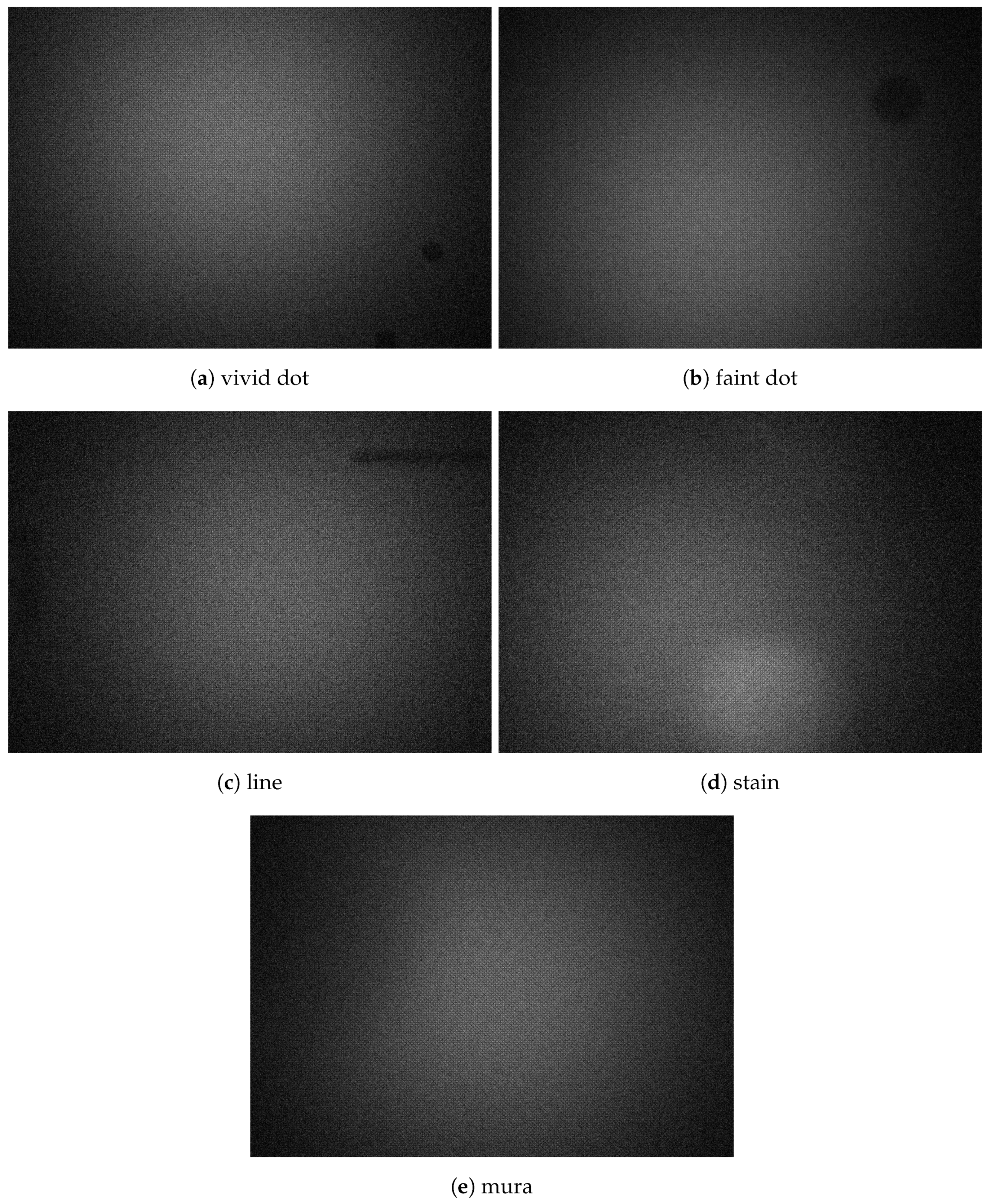
| Vivid Dot | Faint Dot | Line | Stain | Mura | |
|---|---|---|---|---|---|
| Shape | square or circle | square or circle | vertical or horizontal line | ellipse | irregular |
| Range of size | diameter or one side: [11, 14] | diameter or one side: [11, 14] | width: [4, 7] length: [2/3 of vertical or horizontal side of image, half of vertical or horizontal side of image] | length of minor axis: [40, 100] | maximum size: half of image |
| Range of pixel intensities | [40, 44] | [35, 40] | [20, 44] | [15, 25] | [13, 20] |
| Type of smoothing | none | Gaussian | Gaussian or none | Gaussian | Gaussian |
| Range of variance of smoothing filter | none | [3, 30] | [3, 30] | [3, 30] | [5, 30] |
| Range of size of smoothing filter | none | [2, 5] | [2, 5] | [20, 30] | [30, 40] |
| LRS | SBS | PRRS ( = 0) | PRRS ( = 1) | |
|---|---|---|---|---|
| MAE of all region | 4.430 | 0.566 | 0.152 | 0.116 |
| MAE of defective region | 15.458 | 25.306 | 6.080 | 5.594 |
| MAE of sound region | 4.314 | 0.157 | 0.068 | 0.029 |
| Mean of Dice | 0.101 | 0.785 | 0.747 | 0.771 |
| Dice of defective region | 0.037 | 0.580 | 0.501 | 0.548 |
| Dice of sound region | 0.165 | 0.991 | 0.993 | 0.994 |
| Mean of IoU | 0.057 | 0.745 | 0.709 | 0.739 |
| IoU of defective region | 0.023 | 0.504 | 0.430 | 0.487 |
| IoU of sound region | 0.091 | 0.986 | 0.989 | 0.990 |
| = 0.001 | = 0.01 | = 0.1 | = 1 | |
|---|---|---|---|---|
| MAE of all region | 0.116 | 0.112 | 0.112 | 0.111 |
| MAE of defective region | 5.594 | 7.284 | 8.001 | 7.523 |
| MAE of sound region | 0.029 | 0.021 | 0.014 | 0.022 |
| Mean of Dice | 0.771 | 0.759 | 0.753 | 0.753 |
| Dice of defective region | 0.548 | 0.524 | 0.510 | 0.512 |
| Dice of sound region | 0.994 | 0.994 | 0.996 | 0.994 |
| Mean of IoU | 0.739 | 0.723 | 0.712 | 0.715 |
| IoU of defective region | 0.487 | 0.456 | 0.433 | 0.441 |
| IoU of sound region | 0.990 | 0.989 | 0.992 | 0.990 |
| = 0 | = 0.5 | = 1 | = 2 | |
|---|---|---|---|---|
| MAE of all region | 0.152 | 0.113 | 0.116 | 0.118 |
| MAE of defective region | 6.080 | 6.108 | 5.594 | 6.372 |
| MAE of sound region | 0.068 | 0.026 | 0.029 | 0.027 |
| Mean of Dice | 0.747 | 0.734 | 0.771 | 0.798 |
| Dice of defective region | 0.501 | 0.474 | 0.548 | 0.604 |
| Dice of sound region | 0.993 | 0.993 | 0.994 | 0.993 |
| Mean of IoU | 0.709 | 0.692 | 0.739 | 0.768 |
| IoU of defective region | 0.430 | 0.397 | 0.487 | 0.546 |
| IoU of sound region | 0.989 | 0.988 | 0.990 | 0.989 |
| Original Dataset | Shaded and Noised Dataset | |
|---|---|---|
| MAE of all region | 0.116 | 0.271 |
| MAE of defective region | 5.594 | 10.597 |
| MAE of sound region | 0.029 | 0.066 |
| Mean of Dice | 0.771 | 0.726 |
| Dice of defective region | 0.548 | 0.467 |
| Dice of sound region | 0.994 | 0.985 |
| Mean of IoU | 0.739 | 0.682 |
| IoU of defective region | 0.487 | 0.392 |
| IoU of sound region | 0.990 | 0.973 |
| Type of Experiment | Average Computation Time (per Image) |
|---|---|
| LRS | 183 ms |
| PRRS | 313 ms |
© 2019 by the authors. Licensee MDPI, Basel, Switzerland. This article is an open access article distributed under the terms and conditions of the Creative Commons Attribution (CC BY) license (http://creativecommons.org/licenses/by/4.0/).
Share and Cite
Jo, H.; Kim, J. Regularized Auto-Encoder-Based Separation of Defects from Backgrounds for Inspecting Display Devices. Electronics 2019, 8, 533. https://doi.org/10.3390/electronics8050533
Jo H, Kim J. Regularized Auto-Encoder-Based Separation of Defects from Backgrounds for Inspecting Display Devices. Electronics. 2019; 8(5):533. https://doi.org/10.3390/electronics8050533
Chicago/Turabian StyleJo, Heeyeon, and Jeongtae Kim. 2019. "Regularized Auto-Encoder-Based Separation of Defects from Backgrounds for Inspecting Display Devices" Electronics 8, no. 5: 533. https://doi.org/10.3390/electronics8050533
APA StyleJo, H., & Kim, J. (2019). Regularized Auto-Encoder-Based Separation of Defects from Backgrounds for Inspecting Display Devices. Electronics, 8(5), 533. https://doi.org/10.3390/electronics8050533