Some Structures of Parallel VLSI-Oriented Processing Units for Implementation of Small Size Discrete Fractional Fourier Transforms

Abstract

Discrete orthogonal transforms such as the discrete Fourier transform, discrete cosine transform, discrete Hartley transform, etc., are important tools in numerical analysis, signal processing, and statistical methods. The successful application of transform techniques relies on the existence of efficient fast algorithms for their implementation. A special place in the list of transformations is occupied by the discrete fractional Fourier transform (DFrFT). In this paper, some parallel algorithms and processing unit structures for fast DFrFT implementation are proposed. The approach is based on the resourceful factorization of DFrFT matrices. Some parallel algorithms and processing unit structures for small size DFrFTs such as N = 2, 3, 4, 5, 6, and 7 are presented. In each case, we describe only the most important part of the structures of the processing units, neglecting the description of the auxiliary units and the control circuits.

1. Introduction

Traditional discrete orthogonal transforms such as the discrete Fourier transform (DFT), discrete cosine transform (DCT), the discrete Hartley transform (DHT), discrete Walsh–Hadamard transform (DWHT), discrete Haar transform (DHT), and the Slant transform (ST) are important tools in signal and image processing, numerical analysis, and statistical methods. Discrete fractional transforms are another important type of discrete orthogonal transformation. Discrete fractional transforms are the generalizations of the ordinary discrete transforms with one additional fractional parameter. Various discrete fractional transforms including the discrete Fourier transform [1,2,3], the discrete fractional Hartley transform [4], and the discrete fractional cosine and sine transforms [5] have been introduced and found wide applications in many scientific and technological areas including digital signal processing [4], image encryption [6,7,8], digital watermarking [9], and others. Different fast algorithms for their implementation have been separately developed to minimize computational complexity and implementation costs. A striking example is the discrete fractional Fourier transform (DFrFT), the discrete version of the integral fractional Fourier transform (FrFT). Besides its numerical side appropriateness, the DFrFT has proven over the years to be a powerful signal processing tool.

Today, there are many types of definitions of DFrFT. A first approach is represented by direct sampling of the FrFT [10]. It is the least complicated approach, and there are a few different algorithms that have been developed for computing this type of DFrFT. But these discrete realizations could lose many important properties of the FrFT like unitarity, reversibility, additivity; therefore, its applications are limited. A second approach relies on a linear combination of ordinary Fourier operators raised to different powers [11,12]. However, as emphasized in [3], these realizations often produce an output that does not match the output of the continuous FrFT. In other words, it is not the discrete version of the continuous transform. The third approach is based on the idea of an eigenvalue decomposition [1,2,3].

A decisive factor for applications of the various types of DFrFT has been the existence of fast algorithms for computing it. However, only DFrFT based on the eigenvalue decomposition [1,2,3] has all the properties which are required for DFrFT such as unitarity, additivity, reduction to discrete Fourier transform when the power is equal to 1, an approximation of the continuous FrFT [3]. We will call this type of DFrFT as “true” [13]. Fast algorithms for this type of transformation were described in papers [5,14]. The limited volume of these publications did not allow the presentation of all the details of the organization of the calculations for the specific lengths of the original data sequences. In particular, the fast algorithms and schemes for discrete orthogonal transformations for short lengths of input sequences are of practical interest. For example, in [15] the fast algorithms for small-size DFTs were presented. In [16], some schemes for small-size DHTs are given. In the case of DFrFT, such algorithms are not given anywhere. We want to eliminate this shortcoming. To this end, we present fast algorithms and processing unit structures to compute a true DFrFT for N = 2, 3, 4, 5, 6, and 7.

2. Preliminary Remarks

The definition of true DFrFT was first introduced by Pei and Yeh [1,2]. They defined the DFrFT in terms of a particular set of eigenvectors, which constitute the discrete counterpart of the set of Hermite–Gaussian functions (these functions are well-known eigenfunctions of DFT, and the fractional Fourier transform was defined through a spectral expansion in this base [3]):

$${\mathbf{Y}}_{N\times 1}={\mathbf{F}}_N^{\alpha }{\mathbf{X}}_{N\times 1},$$

(1)

where ${\mathbf{F}}_N^{\alpha }$—is $\left(N\times N\right)$ discrete fractional Fourier transform matrix, ${\mathbf{X}}_{N\times 1}={[x_0,x_1,\dots ,x_{N-1}]}^{\mathrm{T}}$, and ${\mathbf{Y}}_{N\times 1}={[y_0,y_1,\dots ,y_{N-1}]}^{\mathrm{T}}$—are input and output data vectors, respectively, and $\alpha$ is a fractional parameter (real number).

The fractional power of the matrix, including the DFT matrix, can be obtained from its eigenvalue decomposition and the power of eigenvalues:

$${\mathbf{F}}_N^{\alpha }={\mathbf{Z}}_N{\mathbf{\Lambda }}_N^{\alpha }{\mathbf{Z}}_N^{\mathrm{T}},$$

(2)

where ${\mathbf{\Lambda }}_N^{\alpha }$ is the diagonal matrix of size N, whose diagonal entries are powers of eigenvalues of the DFT matrix with an exponent α, while ${\mathbf{Z}}_N$ is the matrix whose columns are normalized mutually orthogonal eigenvectors of the DFT matrix.

It is easy to check that the DFrFT matrix, calculated from (2), is symmetric [14]. Moreover the first row (and column) of the matrix ${\mathbf{F}}_N^{\alpha }$ is an even vector and a matrix which we obtain after removing the first row and the first column from the matrix ${\mathbf{F}}_N^{\alpha }$ is persymmetric [14]. Based on that general considerations, we can describe the entries of the DFrFT matrix in the following way:

$${\mathbf{F}}_N^{\alpha }=\left[\begin{array}{cccc}{f}_{0,0}^{\left(\alpha \right)}& f_{0,1}^{\left(\alpha \right)}& \cdots & f_{0,1}^{\left(\alpha \right)}\\ f_{0,1}^{\left(\alpha \right)}& f_{1,1}^{\left(\alpha \right)}& \cdots & f_{1,N-1}^{\left(\alpha \right)}\\ ⋮& ⋮& \ddots & ⋮\\ f_{0,1}^{\left(\alpha \right)}& f_{1,N-1}^{\left(\alpha \right)}& \cdots & f_{1,1}^{\left(\alpha \right)}\end{array}\right]$$

(3)

The entries of this matrix are complex numbers, and their values depend on both the fractional parameter $\alpha$ and the number N. However, it will be more convenient for us to denote the numerical values of the matrix entries by means of the letters of the ordinary Latin alphabet $\{a_N^{\left(\alpha \right)},b_N^{\left(\alpha \right)},c_N^{\left(\alpha \right)},\dots ,z_N^{\left(\alpha \right)}\}$. In this case, the subscript N will indicate the size of the DFrFT matrix, while the superscript α will indicate the value of the fractional parameter. This will simplify the identification of the structural features of the matrix and the presence in it of compositions of the same values of the entries.

3. Algorithm and Processing Unit Structure for Small Size DFrFTs

3.1. Computing the Two-Point DFrFT

Let ${\mathbf{X}}_{2\times 1}={[x_0,x_1]}^{\mathrm{T}}$ and ${\mathbf{Y}}_{2\times 1}={[y_0,y_1]}^{\mathrm{T}}$ be two-dimensional input and output data vectors, respectively.

The problem is to calculate a product

$${\mathbf{Y}}_{2\times 1}={\mathbf{F}}_2^{\alpha }{\mathbf{X}}_{2\times 1},$$

(4)

where

$${\mathbf{F}}_2^{\alpha }=\left[\begin{array}{cc}{a}_2^{\left(\alpha \right)}& b_2^{\left(\alpha \right)}\\ b_2^{\left(\alpha \right)}& c_2^{\left(\alpha \right)}\end{array}\right].$$

Direct computation of (4) takes four multiplications and two additions of complex numbers. From the symmetry of the DFrFT matrix follows that for any value of the parameter $\alpha$, the matrix ${\mathbf{F}}_2^{\alpha }$ contains the same elements on the secondary diagonal. Therefore [17], the number of multiplications in the calculation of the two-point DFrFT can be reduced.

With this in mind, the rationalized computational procedure for computing the two-point DFrFT has the following form:

$${\mathbf{Y}}_{2\times 1}={\mathbf{T}}_{2\times 3}{\mathbf{D}}_3^{\left(\alpha \right)}{\mathbf{T}}_{3\times 2}{\mathbf{X}}_{2\times 1},$$

(5)

where

$${\mathbf{T}}_{3\times 2}=\left[\begin{array}{cc}1& \\ 1& 1\\ & 1\end{array}\right],{\mathbf{T}}_{2\times 3}=\left[\begin{array}{ccc}1& 1& \\ & 1& 1\end{array}\right],{\mathbf{D}}_3^{\left(\alpha \right)}=diag({\stackrel{⏜}{\phi }}_2^{\left(\alpha \right)},b_2^{\left(\alpha \right)},{\breve{\phi }}_2^{\left(\alpha \right)}),$$

and

$${\stackrel{⏜}{\phi }}_2^{\left(\alpha \right)}=a_2^{\left(\alpha \right)}-b_2^{\left(\alpha \right)},{\breve{\phi }}_2^{\left(\alpha \right)}=c_2^{\left(\alpha \right)}-b_2^{\left(\alpha \right)}.$$

As can be seen, the implementation of the two-point DFrFT requires only three multipliers and three two-input adders of complex numbers.

Figure 1 shows a data flow structure for the implementation of the two-point DFrFT. In this paper, data flow structures are oriented from left to right. Straight lines in the figures denote the operations of data transfer. The circles in these figures indicate complex-valued multipliers. These blocks multiply the input data by the numbers inscribed inside the circles. Points where lines converge denote summation and dotted lines indicate the sign-change operations. We use the usual lines without arrows on purpose, so as not to clutter the picture.

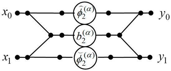
Figure 1. The data flow structure of the proposed algorithm for the computation of the two-point DFrFT.

3.2. Computing the Three-Point DFrFT

Let ${\mathbf{X}}_{3\times 1}={[x_0,x_1,x_2]}^{\mathrm{T}}$ and ${\mathbf{Y}}_{3\times 1}={[y_0,y_1,y_2]}^{\mathrm{T}}$ be three-dimensional input and output data vectors, respectively.

The three-point DFrFT can be represented in the following form:

$${\mathbf{Y}}_{3\times 1}={\mathbf{F}}_3^{\alpha }{\mathbf{X}}_{3\times 1},$$

(6)

where

$${\mathbf{F}}_3^{\alpha }=\left[\begin{array}{ccc}{a}_3^{\left(\alpha \right)}& b_3^{\left(\alpha \right)}& b_3^{\left(\alpha \right)}\\ b_3^{\left(\alpha \right)}& c_3^{\left(\alpha \right)}& d_3^{\left(\alpha \right)}\\ b_3^{\left(\alpha \right)}& d_3^{\left(\alpha \right)}& c_3^{\left(\alpha \right)}\end{array}\right].$$

Taking into account the specific structure of the matrix ${\mathbf{F}}_3^{\alpha },$ we can propose the following procedure for the efficient calculation of a three-point DFrFT:

$${\mathbf{Y}}_{3\times 1}={\mathbf{A}}_{3\times 5}{\mathbf{A}}_5{\mathbf{D}}_5^{\left(\alpha \right)}{\mathbf{P}}_{5\times 3}{\mathbf{A}}_3{\mathbf{X}}_{3\times 1},$$

(7)

where

$${\mathbf{A}}_3=1\oplus {\mathbf{H}}_2=\left[\begin{array}{ccc}1& & \\ & 1& 1\\ & 1& -1\end{array}\right],{\mathbf{P}}_{5\times 3}=\left[\begin{array}{ccc}1& & \\ 1& & \\ & 1& \\ & 1& \\ & & 1\end{array}\right],$$

$${\mathbf{A}}_5={\mathbf{I}}_3\oplus {\mathbf{H}}_2=\left[\begin{array}{ccccc}1& & & & \\ & 1& & & \\ & & 1& & \\ & & & 1& 1\\ & & & 1& -1\end{array}\right],{\mathbf{A}}_{3\times 5}=\left[\begin{array}{ccccc}1& & 1& & \\ & 1& & 1& \\ & 1& & & 1\end{array}\right],$$

$${\mathbf{D}}_5^{\left(\alpha \right)}=diag(a_3^{\left(\alpha \right)},b_3^{\left(\alpha \right)},b_3^{\left(\alpha \right)},{\dot{s}}_3^{\left(\alpha \right)},{\ddot{s}}_3^{\left(\alpha \right)}),$$

$${\dot{s}}_3^{\left(\alpha \right)}=\frac{1}{2}(c_3^{\left(\alpha \right)}+d_3^{\left(\alpha \right)}),{\ddot{s}}_3^{\left(\alpha \right)}=\frac{1}{2}(c_3^{\left(\alpha \right)}-d_3^{\left(\alpha \right)}),$$

and ${\mathit{I}}_N$ is an identity $N\times N$ matrix, ${\mathbf{H}}_2=\left[\begin{array}{cc}1& 1\\ 1& -1\end{array}\right]$ is the (2 × 2) Hadamard matrix, and the sign $\oplus$ denotes the direct sum of two matrices [18].

Figure 2 shows a data flow structure for the implementation of 3-point DFrFT. It is easy to see that the computation of ${\mathbf{Y}}_{3\times 1}$ requires only five multipliers and seven two-input adders of complex numbers.

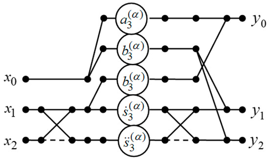
Figure 2. The data flow structure of the proposed algorithm for the computation of the three-point DFrFT.

3.3. Computing the Four-Point DFrFT

Let ${\mathbf{X}}_{4\times 1}={[x_0,x_1,x_2,x_3]}^{\mathrm{T}}$ and ${\mathbf{Y}}_{4\times 1}={[y_0,y_1,y_2,y_3]}^{\mathrm{T}}$ be four-dimensional input and output data vectors, respectively.

The four-point DFrFT can be represented in the following form:

$${\mathbf{Y}}_{4\times 1}={\mathbf{F}}_4^{\alpha }{\mathbf{X}}_{4\times 1},$$

(8)

where

$${\mathbf{F}}_4^{\alpha }=\left[\begin{array}{cccc}{a}_4^{\left(\alpha \right)}& b_4^{\left(\alpha \right)}& c_4^{\left(\alpha \right)}& b_4^{\left(\alpha \right)}\\ b_4^{\left(\alpha \right)}& d_4^{\left(\alpha \right)}& e_4^{\left(\alpha \right)}& f_4^{\left(\alpha \right)}\\ c_4^{\left(\alpha \right)}& e_4^{\left(\alpha \right)}& g_4^{\left(\alpha \right)}& e_4^{\left(\alpha \right)}\\ b_4^{\left(\alpha \right)}& f_4^{\left(\alpha \right)}& e_4^{\left(\alpha \right)}& d_4^{\left(\alpha \right)}\end{array}\right].$$

Taking into account the specific structure of the matrix ${\mathbf{F}}_4^{\alpha }$, we can propose the following procedure for the efficient calculation of a four-point DFrFT:

$${\mathit{Y}}_{4\times 1}={\mathbf{P}}_4^{\mathrm{T}}{\mathit{A}}_{4\times 7}{\mathit{A}}_{7\times 10}{\mathit{D}}_{10}^{\left(\alpha \right)}{\mathit{P}}_{10\times 4}{\mathit{A}}_4{\mathit{P}}_4{\mathit{X}}_{4\times 1},$$

(9)

where

$${\mathbf{P}}_4=\left[\begin{array}{cccc}& & 1& \\ 1& & & \\ & 1& & \\ & & & 1\end{array}\right],{\mathbf{A}}_4={\mathbf{I}}_2\oplus {\mathbf{H}}_2=\left[\begin{array}{cccc}1& & & \\ & 1& & \\ & & 1& 1\\ & & 1& -1\end{array}\right],$$

$${\mathbf{P}}_{10\times 4}=1_{3\times 1}\oplus 1_{3\times 1}\oplus 1_{3\times 1}\oplus 1=\left[\begin{array}{cccc}1& & & \\ 1& & & \\ 1& & & \\ & 1& & \\ & 1& & \\ & 1& & \\ & & 1& \\ & & 1& \\ & & 1& \\ & & & 1\end{array}\right],$$

$${\mathbf{A}}_{7\times 10}=\left[\begin{array}{cccccccccc}1& & & & & & & & & \\ & & 1& & & 1& & 1& & \\ & & & 1& & & & & & \\ & 1& & & 1& & & & & \\ & & & & & & 1& & & \\ & & & & & & & & 1& 1\\ & & & & & & & & 1& -1\end{array}\right],$$

$${\mathbf{A}}_{4\times 7}=\left[\begin{array}{ccccccc}& 1& & & & & \\ 1& & 1& & 1& & \\ & & & 1& & 1& \\ & & & 1& & & 1\end{array}\right],$$

$${\mathbf{D}}_{10}^{\left(\alpha \right)}=diag\left(c_4^{\left(\alpha \right)},e_4^{\left(\alpha \right)},g_4^{\left(\alpha \right)},a_4^{\left(\alpha \right)},b_4^{\left(\alpha \right)},c_4^{\left(\alpha \right)},b_4^{\left(\alpha \right)},e_4^{\left(\alpha \right)}{\dot{s}}_4^{\left(\alpha \right)},{\ddot{s}}_4^{\left(\alpha \right)}\right),$$

$${\dot{s}}_4^{\left(\alpha \right)}=\frac{1}{2}\left(d_4^{\left(\alpha \right)}+f_4^{\left(\alpha \right)}\right),{\ddot{s}}_4^{\left(\alpha \right)}=\frac{1}{2}\left(d_4^{\left(\alpha \right)}-f_4^{\left(\alpha \right)}\right),$$

where $1_{M\times N}$ is an $\left(M\times N\right)$ matrix of ones (a matrix in which every entry is equal to one).

Figure 3 shows a data flow structure for the implementation of a four-point DFrFT. It is easy to see that the computation of ${\mathbf{Y}}_{4\times 1}$ requires only 10 multipliers, seven two-input adders, and two three-inputs adders of complex numbers.

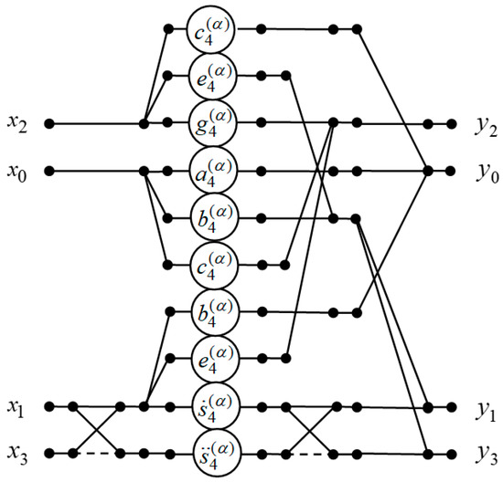
Figure 3. The data flow structure of the processing unit for the computation of the four-point DFrFT.

3.4. Computing the Five-Point DFrFT

Let ${\mathbf{X}}_{5\times 1}={[x_0,x_1,x_2,x_3,x_4]}^{\mathrm{T}}$ and ${\mathbf{Y}}_{5\times 1}={[y_0,y_1,y_2,y_3,x_4]}^{\mathrm{T}}$ be five-dimensional input and output data vectors, respectively.

The five-point DFrFT can be represented in the following form:

$${\mathbf{Y}}_{5\times 1}={\mathbf{F}}_5^{\alpha }{\mathbf{X}}_{5\times 1},$$

(10)

where

$${\mathbf{F}}_5^{\alpha }=\left[\begin{array}{ccccc}{a}_5^{\left(\alpha \right)}& b_5^{\left(\alpha \right)}& c_5^{\left(\alpha \right)}& c_5^{\left(\alpha \right)}& b_5^{\left(\alpha \right)}\\ b_5^{\left(\alpha \right)}& d_5^{\left(\alpha \right)}& e_5^{\left(\alpha \right)}& f_5^{\left(\alpha \right)}& g_5^{\left(\alpha \right)}\\ c_5^{\left(\alpha \right)}& e_5^{\left(\alpha \right)}& h_5^{\left(\alpha \right)}& i_5^{\left(\alpha \right)}& f_5^{\left(\alpha \right)}\\ c_5^{\left(\alpha \right)}& f_5^{\left(\alpha \right)}& i_5^{\left(\alpha \right)}& h_5^{\left(\alpha \right)}& e_5^{\left(\alpha \right)}\\ b_5^{\left(\alpha \right)}& g_5^{\left(\alpha \right)}& f_5^{\left(\alpha \right)}& e_5^{\left(\alpha \right)}& d_5^{\left(\alpha \right)}\end{array}\right].$$

Taking into account the specific structure of the matrix ${\mathbf{F}}_5^{\alpha }$, we can propose the following procedure for the efficient calculation of a five-point DFrFT:

$${\mathbf{Y}}_{5\times 1}={\mathbf{P}}_5^{\mathrm{T}}{\mathbf{A}}_{5\times 7}{\mathbf{A}}_{7\times 9}{\mathbf{P}}_9{\mathbf{A}}_{9\times 11}{\mathbf{D}}_{11}^{\left(\alpha \right)}{\mathbf{A}}_{11\times 9}{\mathbf{P}}_{9\times 5}{\mathbf{A}}_5{\mathbf{P}}_5{\mathbf{X}}_{5\times 1},$$

(11)

where

$${\mathbf{P}}_5=\left[\begin{array}{ccccc}1& & & & \\ & 1& & & \\ & & & & 1\\ & & 1& & \\ & & & 1& \end{array}\right],{\mathbf{A}}_5=\left[\begin{array}{ccccc}1& & & & \\ & 1& 1& & \\ & 1& -1& & \\ & & & 1& 1\\ & & & 1& -1\end{array}\right],{\mathbf{P}}_{9\times 5}=\left[\begin{array}{ccccc}1& & & & \\ 1& & & & \\ 1& & & & \\ & 1& & & \\ & & & 1& \\ & 1& & & \\ & & & 1& \\ & & 1& & \\ & & & & 1\end{array}\right],$$

$${\mathbf{A}}_{11\times 9}=\left[\begin{array}{ccccccccc}1& & & & & & & & \\ & 1& & & & & & & \\ & & 1& & & & & & \\ & & & 1& & & & & \\ & & & & 1& & & & \\ & & & & & 1& & & \\ & & & & & 1& 1& & \\ & & & & & & 1& & \\ & & & & & & & 1& \\ & & & & & & & 1& 1\\ & & & & & & & & 1\end{array}\right],$$

$${\mathbf{A}}_{9\times 11}=\left[\begin{array}{ccccccccccc}1& & & & & & & & & & \\ & 1& & & & & & & & & \\ & & 1& & & & & & & & \\ & & & 1& & & & & & & \\ & & & & 1& & & & & & \\ & & & & & 1& 1& & & & \\ & & & & & & 1& 1& & & \\ & & & & & & & & 1& 1& \\ & & & & & & & & & 1& 1\end{array}\right],$$

$${\mathbf{P}}_9=\left[\begin{array}{ccccccccc}1& & & & & & & & \\ & 1& & & & & & & \\ & & 1& & & & & & \\ & & & 1& & & & & \\ & & & & 1& & & & \\ & & & & & 1& & & \\ & & & & & & & 1& \\ & & & & & & 1& & \\ & & & & & & & & 1\end{array}\right],$$

$${\mathbf{A}}_{7\times 9}=\left[\begin{array}{ccccccccc}1& & & 1& 1& & & & \\ & 1& & & & & & & \\ & & 1& & & & & & \\ & & & & & 1& 1& & \\ & & & & & 1& -1& & \\ & & & & & & & 1& 1\\ & & & & & & & 1& -1\end{array}\right],$$

$${\mathbf{A}}_{5\times 7}=\left[\begin{array}{ccccccc}1& & & & & & \\ & 1& & 1& & & \\ & 1& & & 1& & \\ & & 1& & & 1& \\ & & 1& & & & 1\end{array}\right],$$

$${\mathbf{D}}_{11}^{\left(\alpha \right)}=diag(a_5^{\left(\alpha \right)},b_5^{\left(\alpha \right)},c_5^{\left(\alpha \right)},b_5^{\left(\alpha \right)},c_5^{\left(\alpha \right)},{\breve{s}}_5^{\left(\alpha \right)},{\stackrel{⏜}{s}}_5^{\left(\alpha \right)},{\tilde{s}}_5^{\left(\alpha \right)}{\dot{s}}_5^{\left(\alpha \right)},{\ddot{s}}_5^{\left(\alpha \right)},{\stackrel{⃛}{s}}_5^{\left(\alpha \right)}),$$

$${\breve{s}}_5^{\left(\alpha \right)}=\frac{1}{2}(d_5^{\left(\alpha \right)}-e_5^{\left(\alpha \right)}+g_5^{\left(\alpha \right)}-f_5^{\left(\alpha \right)}),{\stackrel{⏜}{s}}_5^{\left(\alpha \right)}=\frac{1}{2}(e_5^{\left(\alpha \right)}+f_5^{\left(\alpha \right)}),$$

$${\tilde{s}}_5^{\left(\alpha \right)}=\frac{1}{2}(h_5^{\left(\alpha \right)}-e_5^{\left(\alpha \right)}+i_5^{\left(\alpha \right)}-f_5^{\left(\alpha \right)}),{\dot{s}}_5^{\left(\alpha \right)}=\frac{1}{2}(d_5^{\left(\alpha \right)}-e_5^{\left(\alpha \right)}-g_5^{\left(\alpha \right)}+f_5^{\left(\alpha \right)}),$$

$${\ddot{s}}_5^{\left(\alpha \right)}=\frac{1}{2}(e_5^{\left(\alpha \right)}-f_5^{\left(\alpha \right)}),{\stackrel{⃛}{s}}_5^{\left(\alpha \right)}=\frac{1}{2}(h_5^{\left(\alpha \right)}-e_5^{\left(\alpha \right)}-i_5^{\left(\alpha \right)}+f_5^{\left(\alpha \right)}).$$

Figure 4 shows a data flow structure for the implementation of 5-point DFrFT. It is easy to see that the computation of ${\mathbf{Y}}_{5\times 1}$ requires only 11 multipliers, 18 two-input adders, and 1 three-input adder of complex numbers.

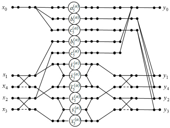
Figure 4. The data flow structure of the processing unit for computation of 5-point DFrFT.

3.5. Computing the 6-Point DFrFT

Let ${\mathbf{X}}_{6\times 1}={[x_0,x_1,x_2,x_3,x_4,x_5]}^{\mathrm{T}}$ and ${\mathbf{Y}}_{6\times 1}={[y_0,y_1,y_2,y_3,x_4,x_5]}^{\mathrm{T}}$ be six-dimensional input and output data vectors, respectively.

The 6-point DFrFT can be represented in the following form:

$${\mathbf{Y}}_{6\times 1}={\mathbf{F}}_6^{\alpha }{\mathbf{X}}_{6\times 1},$$

(12)

where

$${\mathbf{F}}_6^{\alpha }=\left[\begin{array}{cccccc}{a}_6^{\left(\alpha \right)}& b_6^{\left(\alpha \right)}& c_6^{\left(\alpha \right)}& d_6^{\left(\alpha \right)}& c_6^{\left(\alpha \right)}& b_6^{\left(\alpha \right)}\\ b_6^{\left(\alpha \right)}& f_6^{\left(\alpha \right)}& g_6^{\left(\alpha \right)}& e_6^{\left(\alpha \right)}& h_6^{\left(\alpha \right)}& i_6^{\left(\alpha \right)}\\ c_6^{\left(\alpha \right)}& g_6^{\left(\alpha \right)}& j_6^{\left(\alpha \right)}& k_6^{\left(\alpha \right)}& l_6^{\left(\alpha \right)}& h_6^{\left(\alpha \right)}\\ d_6^{\left(\alpha \right)}& e_6^{\left(\alpha \right)}& k_6^{\left(\alpha \right)}& m_6^{\left(\alpha \right)}& k_6^{\left(\alpha \right)}& e_6^{\left(\alpha \right)}\\ c_6^{\left(\alpha \right)}& h_6^{\left(\alpha \right)}& l_6^{\left(\alpha \right)}& k_6^{\left(\alpha \right)}& j_6^{\left(\alpha \right)}& g_6^{\left(\alpha \right)}\\ b_6^{\left(\alpha \right)}& i_6^{\left(\alpha \right)}& h_6^{\left(\alpha \right)}& e_6^{\left(\alpha \right)}& g_6^{\left(\alpha \right)}& f_6^{\left(\alpha \right)}\end{array}\right]$$

Taking into account the specific structure of the matrix ${\mathbf{F}}_6^{\alpha }$, we can propose the following procedure for the efficient calculation of a 6-point DFrFT:

$${\mathbf{Y}}_{6\times 1}={\mathbf{P}}_6^{\mathrm{T}}{\mathbf{A}}_{6\times 8}{\mathbf{A}}_{8\times 11}{\mathbf{P}}_{11}{\mathbf{A}}_{11\times 18}{\mathbf{D}}_{18}^{\left(\alpha \right)}{\mathbf{A}}_{18\times 16}{\mathbf{P}}_{16\times 6}{\mathbf{A}}_6{\mathbf{P}}_6{\mathbf{X}}_{6\times 1},$$

(13)

where

$${\mathbf{P}}_6=\left[\begin{array}{cccccc}& & & 1& & \\ 1& & & & & \\ & 1& & & & \\ & & & & & 1\\ & & 1& & & \\ & & & & 1& \end{array}\right],{\mathbf{A}}_6={\mathbf{I}}_2\oplus {\mathbf{H}}_2\oplus {\mathbf{H}}_2=\left[\begin{array}{cccccc}1& & & & & \\ & 1& & & & \\ & & 1& 1& & \\ & & 1& -1& & \\ & & & & 1& 1\\ & & & & 1& -1\end{array}\right],$$

$${\mathbf{P}}_{16\times 6}=1_{4\times 1}\oplus 1_{4\times 1}\oplus \left[\begin{array}{cccc}1& & & \\ 1& & & \\ & & 1& \\ & & 1& \\ 1& & & \\ & & 1& \\ & 1& & \\ & & & 1\end{array}\right],{\mathbf{A}}_{18\times 16}={\mathbf{I}}_{12}\oplus \left[\begin{array}{cccc}1& & & \\ 1& 1& & \\ & 1& & \\ & & 1& \\ & & 1& 1\\ & & & 1\end{array}\right],$$

$${\mathbf{A}}_{11\times 18}=\left[\begin{array}{cccccccccccc}1& & & & & & & & & & & \\ & & & 1& & & & 1& 1& & 1& \\ & & & & 1& & & & & & & \\ & 1& & & & 1& & & & & & \\ & & 1& & & & 1& & & & & \\ & & & & & & & & & 1& & \\ & & & & & & & & & & & 1\end{array}\right]\oplus \left[\begin{array}{cccccc}1& 1& & & & \\ & 1& 1& & & \\ & & & 1& 1& \\ & & & & 1& 1\end{array}\right],$$

$${\mathbf{P}}_{11}={\mathbf{I}}_7\oplus \left[\begin{array}{cccc}1& & & \\ & & 1& \\ & 1& & \\ & & & 1\end{array}\right],$$

$${\mathbf{A}}_{8\times 11}=\left[\begin{array}{ccccccc}& 1& & & & & \\ 1& & & & & 1& 1\\ & & & 1& & & \\ & & & & 1& & \end{array}\right]\oplus {\mathbf{H}}_2\oplus {\mathbf{H}}_2,$$

$${\mathbf{A}}_{6\times 8}=\left[\begin{array}{cccccccc}1& & & & & & & \\ & 1& & & & & & \\ & & 1& & 1& & & \\ & & 1& & & 1& & \\ & & & 1& & & 1& \\ & & & 1& & & & 1\end{array}\right],$$

$${\mathbf{D}}_{18}^{\left(\alpha \right)}={\breve{\mathbf{D}}}_{12}^{\left(\alpha \right)}\oplus {\stackrel{⏜}{\mathbf{D}}}_6^{\left(\alpha \right)},$$

$${\breve{\mathbf{D}}}_{12}^{\left(\alpha \right)}=diag\left(d_6^{\left(\alpha \right)},e_6^{\left(\alpha \right)},k_6^{\left(\alpha \right)},m_6^{\left(\alpha \right)},a_6^{\left(\alpha \right)},b_6^{\left(\alpha \right)},c_6^{\left(\alpha \right)},d_6^{\left(\alpha \right)},e_6^{\left(\alpha \right)},b_6^{\left(\alpha \right)},k_6^{\left(\alpha \right)},c_6^{\left(\alpha \right)}\right),$$

$${\stackrel{⏜}{\mathbf{D}}}_6^{\left(\alpha \right)}=diag\left({\breve{s}}_6^{\left(\alpha \right)},{\stackrel{⏜}{s}}_6^{\left(\alpha \right)},{\tilde{s}}_6^{\left(\alpha \right)},{\dot{s}}_6^{\left(\alpha \right)},{\ddot{s}}_6^{\left(\alpha \right)},{\stackrel{⃛}{s}}_6^{\left(\alpha \right)}\right),$$

$${\breve{s}}_6^{\left(\alpha \right)}=\frac{1}{2}\left(f_6^{\left(\alpha \right)}-g_6^{\left(\alpha \right)}+i_6^{\left(\alpha \right)}-h_6^{\left(\alpha \right)}\right),{\stackrel{⏜}{s}}_6^{\left(\alpha \right)}=\frac{1}{2}\left(g_6^{\left(\alpha \right)}+h_6^{\left(\alpha \right)}\right),$$

$${\tilde{s}}_6^{\left(\alpha \right)}=\frac{1}{2}\left(j_6^{\left(\alpha \right)}-g_6^{\left(\alpha \right)}+l_6^{\left(\alpha \right)}-h_6^{\left(\alpha \right)}\right),{\dot{s}}_6^{\left(\alpha \right)}=\frac{1}{2}\left(f_6^{\left(\alpha \right)}-g_6^{\left(\alpha \right)}-i_6^{\left(\alpha \right)}+h_6^{\left(\alpha \right)}\right),$$

$${\ddot{s}}_6^{\left(\alpha \right)}=\frac{1}{2}\left(g_6^{\left(\alpha \right)}-h_6^{\left(\alpha \right)}\right),{\stackrel{⃛}{s}}_6^{\left(\alpha \right)}=\frac{1}{2}\left(j_6^{\left(\alpha \right)}-g_6^{\left(\alpha \right)}-l_6^{\left(\alpha \right)}+h_6^{\left(\alpha \right)}\right).$$

Figure 5 shows a data flow structure for the implementation of the six-point DFrFT. It is easy to see that the computation of ${\mathbf{Y}}_{6\times 1}$ requires only 18 multipliers, 20 two-input adders, and two four-input adders of complex numbers.

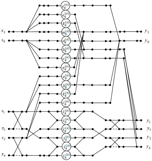
Figure 5. The data flow structure of the processing unit for the computation of the six-point DFrFT.

3.6. Computing th eSeven-Point DFrFT

Let ${\mathbf{X}}_{7\times 1}={[x_0,x_1,x_2,x_3,x_4,x_5,x_6]}^{\mathrm{T}}$ and ${\mathbf{Y}}_{7\times 1}={[y_0,y_1,y_2,y_3,x_4,x_5,x_6]}^{\mathrm{T}}$ be seven-dimensional input and output data vectors, respectively.

The seven-point DFrFT can be represented in the following form:

$${\mathbf{Y}}_{7\times 1}={\mathbf{F}}_7^{\alpha }{\mathbf{X}}_{7\times 1},$$

(14)

where

$${\mathbf{F}}_7^{\alpha }=\left[\begin{array}{ccccccc}{a}_7^{\left(\alpha \right)}& b_7^{\left(\alpha \right)}& c_7^{\left(\alpha \right)}& d_7^{\left(\alpha \right)}& d_7^{\left(\alpha \right)}& c_7^{\left(\alpha \right)}& b_7^{\left(\alpha \right)}\\ b_7^{\left(\alpha \right)}& e_7^{\left(\alpha \right)}& f_7^{\left(\alpha \right)}& g_7^{\left(\alpha \right)}& h_7^{\left(\alpha \right)}& i_7^{\left(\alpha \right)}& j_7^{\left(\alpha \right)}\\ c_7^{\left(\alpha \right)}& f_7^{\left(\alpha \right)}& k_7^{\left(\alpha \right)}& l_7^{\left(\alpha \right)}& m_7^{\left(\alpha \right)}& n_7^{\left(\alpha \right)}& i_7^{\left(\alpha \right)}\\ d_7^{\left(\alpha \right)}& g_7^{\left(\alpha \right)}& l_7^{\left(\alpha \right)}& o_7^{\left(\alpha \right)}& p_7^{\left(\alpha \right)}& m_7^{\left(\alpha \right)}& h_7^{\left(\alpha \right)}\\ d_7^{\left(\alpha \right)}& h_7^{\left(\alpha \right)}& m_7^{\left(\alpha \right)}& p_7^{\left(\alpha \right)}& o_7^{\left(\alpha \right)}& l_7^{\left(\alpha \right)}& g_7^{\left(\alpha \right)}\\ c_7^{\left(\alpha \right)}& i_7^{\left(\alpha \right)}& n_7^{\left(\alpha \right)}& m_7^{\left(\alpha \right)}& l_7^{\left(\alpha \right)}& k_7^{\left(\alpha \right)}& f_7^{\left(\alpha \right)}\\ b_7^{\left(\alpha \right)}& j_7^{\left(\alpha \right)}& i_7^{\left(\alpha \right)}& h_7^{\left(\alpha \right)}& g_7^{\left(\alpha \right)}& f_7^{\left(\alpha \right)}& e_7^{\left(\alpha \right)}\end{array}\right].$$

Taking into account the specific structure of the matrix ${\mathbf{F}}_7^{\alpha }$, we can propose the following procedure for the efficient calculation of a seven-point DFrFT:

$${\mathbf{Y}}_{7\times 1}={\mathbf{P}}_7^{\mathrm{T}}{\mathbf{A}}_{7\times 10}{\mathbf{A}}_{10\times 13}{\mathbf{P}}_{13}{\mathbf{A}}_{13\times 19}{\mathbf{D}}_{19}^{\left(\alpha \right)}{\mathbf{A}}_{19\times 13}{\mathbf{P}}_{13\times 7}{\mathbf{A}}_7{\mathbf{P}}_7{\mathbf{X}}_{7\times 1},$$

(15)

where

$${\mathbf{P}}_7=\left[\begin{array}{ccccccc}1& & & & & & \\ & 1& & & & & \\ & & & & & & 1\\ & & 1& & & & \\ & & & & & 1& \\ & & & 1& & & \\ & & & & 1& & \end{array}\right],$$

$${\mathbf{A}}_7=1\oplus \left({\mathbf{I}}_3\otimes {\mathbf{H}}_2\right)=\left[\begin{array}{ccccccc}1& & & & & & \\ & 1& 1& & & & \\ & 1& -1& & & & \\ & & & 1& 1& & \\ & & & 1& -1& & \\ & & & & & 1& 1\\ & & & & & 1& -1\end{array}\right],$$

$${\mathbf{P}}_{13\times 7}=\left[\begin{array}{ccccccc}1& & & & & & \\ 1& & & & & & \\ 1& & & & & & \\ 1& & & & & & \\ & 1& & & & & \\ & & & 1& & & \\ & & & & & 1& \\ & 1& & & & & \\ & & & 1& & & \\ & & & & & 1& \\ & & 1& & & & \\ & & & & 1& & \\ & & & & & & 1\end{array}\right],{\mathbf{A}}_{19\times 13}={\mathbf{I}}_7\oplus \left[\begin{array}{cccccc}1& & & & & \\ 1& 1& & & & \\ & 1& & & & \\ & 1& 1& & & \\ & & 1& & & \\ 1& & 1& & & \\ & & & 1& & \\ & & & 1& 1& \\ & & & & 1& \\ & & & & 1& 1\\ & & & & & 1\\ & & & 1& & 1\end{array}\right],$$

$${\mathbf{A}}_{13\times 19}={\mathbf{I}}_7\oplus \left[\begin{array}{cccccccccccc}1& 1& & & & 1& & & & & & \\ & 1& 1& 1& & & & & & & & \\ & & & 1& 1& 1& & & & & & \\ & & & & & & 1& 1& & & & 1\\ & & & & & & & 1& 1& 1& & \\ & & & & & & & & & 1& 1& 1\end{array}\right],$$

$${\mathbf{P}}_{13}={\mathbf{I}}_7\oplus \left[\begin{array}{cccccc}1& & & & & \\ & & & 1& & \\ & 1& & & & \\ & & & & 1& \\ & & 1& & & \\ & & & & & 1\end{array}\right],{\mathbf{A}}_{10\times 13}=\left[\begin{array}{ccccccc}1& & & & 1& 1& 1\\ & 1& & & & & \\ & & 1& & & & \\ & & & 1& & & \end{array}\right]\oplus \left({\mathbf{I}}_3\otimes {\mathbf{H}}_2\right),$$

$${\mathbf{A}}_{7\times 10}=\left[\begin{array}{cccccccccc}1& & & & & & & & & \\ & 1& & & 1& & & & & \\ & 1& & & & 1& & & & \\ & & 1& & & & 1& & & \\ & & 1& & & & & 1& & \\ & & & 1& & & & & 1& \\ & & & 1& & & & & & 1\end{array}\right],$$

$${\mathbf{D}}_{19}^{\left(\alpha \right)}={\breve{\mathbf{D}}}_7^{\left(\alpha \right)}\oplus {\stackrel{⏜}{\mathbf{D}}}_{12}^{\left(\alpha \right)},$$

$${\breve{\mathbf{D}}}_7^{\left(\alpha \right)}=diag\left(a_7^{\left(\alpha \right)},b_7^{\left(\alpha \right)},c_7^{\left(\alpha \right)},d_7^{\left(\alpha \right)},b_7^{\left(\alpha \right)},c_7^{\left(\alpha \right)},d_7^{\left(\alpha \right)}\right),$$

$${\stackrel{⏜}{\mathbf{D}}}_{12}^{\left(\alpha \right)}=diag\left({\breve{s}}_7^{\left(\alpha \right)},{\stackrel{⏜}{s}}_7^{\left(\alpha \right)},{\tilde{s}}_7^{\left(\alpha \right)},{\dot{s}}_7^{\left(\alpha \right)},{\ddot{s}}_7^{\left(\alpha \right)},{\stackrel{⃛}{s}}_7^{\left(\alpha \right)},{\overrightarrow{s}}_7^{\left(\alpha \right)},{\overleftarrow{s}}_7^{\left(\alpha \right)},{\overleftrightarrow{s}}_7^{\left(\alpha \right)},{s^{\prime }}_7^{\left(\alpha \right)},{s^{\prime }}_7^{\left(\alpha \right)},{s^{‴}}_7^{\left(\alpha \right)}\right),$$

$${\breve{s}}_7^{\left(\alpha \right)}=\frac{1}{2}\left(e_7^{\left(\alpha \right)}-f_7^{\left(\alpha \right)}-g_7^{\left(\alpha \right)}+j_7^{\left(\alpha \right)}-i_7^{\left(\alpha \right)}-h_7^{\left(\alpha \right)}\right),{\stackrel{⏜}{s}}_7^{\left(\alpha \right)}=\frac{1}{2}\left(f_7^{\left(\alpha \right)}+i_7^{\left(\alpha \right)}\right),$$

$${\tilde{s}}_7^{\left(\alpha \right)}=\frac{1}{2}\left(k_7^{\left(\alpha \right)}-f_7^{\left(\alpha \right)}-l_7^{\left(\alpha \right)}+n_7^{\left(\alpha \right)}-i_7^{\left(\alpha \right)}-m_7^{\left(\alpha \right)}\right),{\dot{s}}_7^{\left(\alpha \right)}=\frac{1}{2}\left(l_7^{\left(\alpha \right)}+m_7^{\left(\alpha \right)}\right),$$

$${\ddot{s}}_7^{\left(\alpha \right)}=\frac{1}{2}\left(o_7^{\left(\alpha \right)}-g_7^{\left(\alpha \right)}-l_7^{\left(\alpha \right)}+p_7^{\left(\alpha \right)}-h_7^{\left(\alpha \right)}-m_7^{\left(\alpha \right)}\right),{\stackrel{⃛}{s}}_7^{\left(\alpha \right)}=\frac{1}{2}\left(g_7^{\left(\alpha \right)}+h_7^{\left(\alpha \right)}\right),$$

$${\overrightarrow{s}}_7^{\left(\alpha \right)}=\frac{1}{2}\left(e_7^{\left(\alpha \right)}-f_7^{\left(\alpha \right)}-g_7^{\left(\alpha \right)}-j_7^{\left(\alpha \right)}+i_7^{\left(\alpha \right)}+h_7^{\left(\alpha \right)}\right),{\overleftarrow{s}}_7^{\left(\alpha \right)}=\frac{1}{2}\left(f_7^{\left(\alpha \right)}-i_7^{\left(\alpha \right)}\right),$$

$${\overleftrightarrow{s}}_7^{\left(\alpha \right)}=\frac{1}{2}\left(k_7^{\left(\alpha \right)}-f_7^{\left(\alpha \right)}-l_7^{\left(\alpha \right)}-n_7^{\left(\alpha \right)}+i_7^{\left(\alpha \right)}+m_7^{\left(\alpha \right)}\right),{s^{\prime }}_7^{\left(\alpha \right)}=\frac{1}{2}\left(l_7^{\left(\alpha \right)}-m_7^{\left(\alpha \right)}\right),$$

$${s^{″}}_7^{\left(\alpha \right)}=\frac{1}{2}\left(o_7^{\left(\alpha \right)}-g_7^{\left(\alpha \right)}-l_7^{\left(\alpha \right)}-p_7^{\left(\alpha \right)}+h_7^{\left(\alpha \right)}+m_7^{\left(\alpha \right)}\right),{s^{‴}}_7^{\left(\alpha \right)}=\frac{1}{2}\left(g_7^{\left(\alpha \right)}-h_7^{\left(\alpha \right)}\right).$$

The sign $\otimes$ denotes the Kronecker product of two matrices [18].

Figure 6 shows a data flow structure for the implementation of the seven-point DFrFT. It is easy to see that the computation of ${\mathbf{Y}}_{7\times 1}$ requires only 19 multipliers and 24 two-input adders, six three-input adders, and one four-input adder of complex numbers.

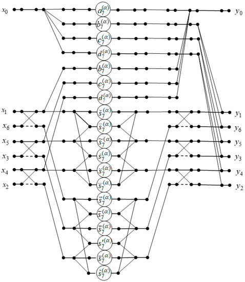
Figure 6. The data flow structure of the processing unit for the computation of the seven-point DFrFT.

4. Implementation Complexity

Since the lengths of the input sequences are relatively small, and the data flow structures representing the organization of the computation process are fairly simple, it is easy to estimate the computational complexity of the implementation of the presented solutions. Table 1 shows evaluations of the number of arithmetic blocks for the small-size DFrFTs hardware implementations.

Table 1. Implementation complexities of naive and proposed solutions.

Size N	Numbers of Arithmetic Blocks
	Naive Method		Proposed Algorithm
	Multipliers	N-Input Adders	Multipliers	2-Input Adders	3-Input Adders	4-Input Adders
2	4	2	3	3	-	-
3	9	3	5	7	-	-
4	16	4	10	7	2	-
5	25	5	11	18	1	-
6	36	6	18	20	-	2
7	49	7	19	24	6	1

5. Discussion

This paper presents some algorithms and parallel processing unit structures for small-size DFrFTs with a minimalized number of complex-valued multiplications (or complex multipliers in the case of a hardware implementation). Special attention is mainly focused on these operations because from the point of view of the hardware implementation complexity; these operations are the most expensive. This is because the complexity of implementing an adder depends linearly on the size of the operand, and the complexity of implementing a multiplier depends quadratically on the size of the operand. A binary multiplier occupies much more space and consumes much more power than a binary adder. Therefore, a processing unit structure containing as few multipliers as possible, even by the cost of a small increase in the number of adders, is preferable from the point of view of the application-specific integrated circuit (ASIC) design. The developed algorithms can be used as building blocks in more complex DSP algorithms. In the case of a hardware implementation of complex signal processing systems, the developed structures can be used as embedded hardware-implemented processing cores. Hopefully, these can be used as building blocks to reduce the hardware complexity of the DSP systems that use them, thus making more complicated structural solutions worthy of consideration in practice.

In our next articles, we plan to show how and for what purposes we use the solutions proposed here.

References

- Pei, S.-C.; Yeh, M.-H. Improved discrete fractional Fourier transform. Opt. Lett. 1997, 22, 1047–1049. [Google Scholar] [CrossRef] [PubMed]
- Pei, S.-C.; Yeh, M.-H.; Tseng, C.-C. Discrete fractional Fourier transform based on orthogonal projections. IEEE Trans. Signal Process. 1999, 47, 1335–1348. [Google Scholar] [CrossRef]
- Candan, Ç.C.; Kutay, M.A.; Ozaktas, H.M. The discrete fractional Fourier transform. IEEE Trans. Signal Process. 2000, 48, 1329–1337. [Google Scholar] [CrossRef]
- Pei, S.-C.; Tseng, C.-C.; Yeh, M.-H.; Shyu, J.-J. Discrete fractional Hartley and Fourier transforms. IEEE Trans. Circuits Syst. II Analog Digit. Signal Process. 1998, 45, 665–675. [Google Scholar] [CrossRef]
- Pei, S.-C.; Yeh, M.H. The discrete fractional cosine and sine transforms. IEEE Trans. Signal Process. 2001, 49, 1198–1207. [Google Scholar] [CrossRef]
- Hennelly, B.; Sheridan, J.T. Fractional Fourier transform-based image encryption: Phase retrieval algorithm. Opt. Commun. 2003, 226, 61–80. [Google Scholar] [CrossRef]
- Liu, S.; Mi, Q.; Zhu, B. Optical image encryption with multistage and multichannel fractional Fourier-domain filtering. Opt. Lett. 2001, 26, 1242–1244. [Google Scholar] [CrossRef] [PubMed]
- Nishchal, N.K.; Joseph, J.; Singh, K. Fully phase encryption using fractional Fourier transform. Opt. Eng. 2003, 42, 1583–1588. [Google Scholar] [CrossRef]
- Djurović, I.; Stanković, S.; Pitas, I. Digital watermarking in the fractional Fourier transformation domain. J. Netw. Comput. Appl. 2001, 24, 167–173. [Google Scholar] [CrossRef]
- Ozaktas, H.M.; Ankan, O.; Kutay, M.A.; Bozdagi, G. Digital computation of the fractional Fourier transform. IEEE Trans. Signal Process. 1996, 44, 2141–2150. [Google Scholar] [CrossRef]
- Santhanam, B.; McClellan, J.H. Discrete rotational Fourier transform. IEEE Trans. Signal Process. 1996, 44, 994–998. [Google Scholar] [CrossRef]
- Dickinson, B.W.; Steiglitz, K. Eigenvectors and functions of the discrete Fourier transform. IEEE Trans. Acoust. Speech Signal Process. 1982, 30, 25–31. [Google Scholar] [CrossRef]
- Majorkowska–Mech, D.; Cariow, A. An Algorithm for Computing the True Discrete Fractional Fourier Transform. In Advances in Soft and Hard Computing; Pejaś, J., El Fray, I., Hyla, T., Kacprzyk, J., Eds.; Springer: Cham, Switzerland, 2019; Volume 889, pp. 420–432. [Google Scholar] [CrossRef]
- Majorkowska–Mech, D.; Cariow, A. A low-complexity approach to computation of the discrete fractional Fourier transform. Circuits Syst. Signal Process. 2017, 36, 4118–4144. [Google Scholar] [CrossRef][Green Version]
- Qureshi, F.; Garrido, M.; Gustafsson, O. Unified architecture for 2, 3, 4, 5, and 7-point DFTs based on Winograd Fourier transform algorithm. Electron. Lett. 2013, 49, 348–349. [Google Scholar] [CrossRef]
- De Oliveira, H.M.; Cintra, R.J.; Campello de Souza, R.M. A Factorization Scheme for Some Discrete Hartley Transform Matrices. arXiv 2015, arXiv:1502.01038, 1–10. [Google Scholar]
- Cariow, A. Strategies for the Synthesis of Fast Algorithms for the Computation of the Matrix-vector Products. J. Signal Process. Theory Appl. 2014, 3, 1–19. [Google Scholar] [CrossRef]
- Graham, A. Kronecker Products and Matrix Calculus: With Applications; Ellis Horwood Limited: Chichester, UK, 1981. [Google Scholar]
© 2019 by the authors. Licensee MDPI, Basel, Switzerland. This article is an open access article distributed under the terms and conditions of the Creative Commons Attribution (CC BY) license (http://creativecommons.org/licenses/by/4.0/).