Abstract
This paper presents the modeling and control-loop design method with an inverted decoupling scheme of a single-phase photovoltaic grid-connected five-level cascaded H-bridge multilevel inverter. For the unity power factor, the proportional and integral current controller with a duty ratio feed-forward compensation is used. In addition, in order to achieve the maximum power point tracking of each photovoltaic array, when the stacked modules are in the partial shading condition, each direct current (DC) voltage is stably controlled to their maximum power points (MPP) by dedicated voltage controllers of each H-bridge module. This paper also presents a control method that minimizes the effect of the loop-interaction in the design of an individual DC-link voltage control loop in a two-input two-output system. The proposed control methods of the cascaded H-bridge multilevel inverter are validated through the simulation and experimental results of the 2-kW prototype hardware.
1. Introduction
The multilevel converter can improve efficiency by enabling the use of components with better characteristics due to the reduced voltage stress, and has the advantage of lowering electromagnetic emissions by providing a staircase output voltage [1,2,3,4,5,6,7,8,9,10]. Thus, the use of a multilevel converter has increased in industrial and renewable energy applications, which require high-voltage and high output quality [11,12,13,14]. In recent times, studies of photovoltaic applications with multilevel topologies have made progress in increasing the efficiency and lowering the electromagnetic interference (EMI) and core losses [10,11,12,13,14,15,16,17]. The multi-level converter has been used mainly in renewable energy systems using high-voltage above kV, but researches are expanding to low-voltage applications to take advantage of the aforementioned merits [16,17]. Among several studies, because isolated direct current (DC) sources are naturally obtained from the photovoltaic (PV) arrays, and can be easily modularized compared to other multilevel converters, a PV generation system with the cascaded H-bridge multilevel inverter topology has been studied [16,17,18,19,20,21,22,23,24,25]. Reference [16] presented a study on the reactive power compensation for the single phase grid-connected cascaded H-bridge multilevel inverter, but they did not fully suggest the method for designing the controller. The results of applying a cascaded H-bridge multilevel inverter to the rooftop photovoltaic micro-inverter as a low-voltage application were studied in [17]. In this paper, they present the results of a power balancing scheme using a multi-level inverter in a two-stage power conversion architecture. However, there is no analysis for control-loop design and only simulation results are presented.
In grid-tied PV generation systems, the single stage structure requires many series-connected PV modules for making PV arrays with a high voltage. However, each of the stacked PV modules has its optimal maximum power points (MPPs) owing to the partial shading when the PV operates under a non-uniform irradiation. When the illumination level is decreased because of non-uniform irradiation, the whole PV system has multiple maximum power points. In this situation, the maximum power point tracking (MPPT) algorithm is apt to fall into the local MPPs and the output power is considerably decreased [26,27,28,29,30,31,32,33].
However, this problem can be mitigated by using the cascaded H-bridge multilevel inverter. When using the cascaded H-bridge multilevel inverter, PV modules are separately divided and grouped by the number of H-bridge modules, and the output voltage of PV arrays can be controlled to achieve their MPPs. Thus, the control loop design should be taken into account, in order to achieve the individual voltage control of each PV array and the unity power factor control in multi-input multi-output systems. In [34], the individual DC-link voltage control and PWM method are proposed in order to achieve the aforementioned objectives. However, the loop-interaction and solutions among H-bridge modules are not presented. Compared with a previous conference paper [35], we further present the inverted decoupling control method and the simulation results to show the effectiveness of the proposed method to minimize the loop gain interactions that occur when controlling each PV array voltage. Furthermore, we describe the detailed modeling process and simulation results for verification of the designed controller that was not presented in the previous paper to make it easier for other researchers to understand. In addition, the MPPT algorithm for tracking the MPPs of the photovoltaic system is further described.
In this paper, the controller design method with an inverted decoupling scheme of the cascaded H-bridge multilevel inverter for achieving an individual MPPT of each PV array and the unity power factor of the grid current is presented. The proportional and integral (PI) current controller, with the duty ratio feed-forward compensation method for minimizing the steady-state error and the phase delay is applied. In addition, in order to avoid a local MPPT, the output voltage of each PV array is individually controlled through the decoupled loop gain design method of the two-input two-output (TITO) system. The proposed small signal modeling and control loop design methods are validated through the simulation and experimental results of the 2-kW five-level single-phase cascaded H-bridge multilevel inverter system.
The remainder of this approach is organized as follows. This approach is divided into four parts including this introduction section. To begin with, the small signal transfer function of the cascaded H-bridge multilevel inverter based on the small signal modeling approaches are derived in Section 2. Also, the current and voltage controller design methods using the inverted decoupling method of two-input two output system are described. Section 3 shows the simulation and experimental setup and the results of the proposed approach. The experimental results show the validity of the proposed individual voltage control for obtaining the maximum power of each PV module. In the final section, some conclusions and final remarks are given.
2. Modeling and Control Loop Design Method
2.1. Small Signal Modeling of Five-Level Cascaded H-bridge Multilevel Inverter
The single-phase five-level cascaded H-bridge multilevel PV system is shown in Figure 1. In order to design the control loops, a small signal model, based on the state space averaging method [36,37], is developed. More detailed small-signal modeling is given in [37]. The input currents and output voltages of each H-bridge power stage of Figure 1 are defined as (1)–(4), using the switching states shown in Figure 2.
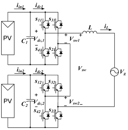
Figure 1.
Single-phase photovoltaic cascaded H-bridge multilevel inverter.
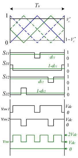
Figure 2.
Relationship of switching states and duty ratios of the cascaded multilevel inverter.
S11 and S31 are switching states of the upper switches of each leg in the upper H-bridge module and can take the values 1 or 0, according to the compared result between the modulating (vc*) and carrier signal, as shown in Figure 2. idc1 and vsw1 are the input current and the output voltage of the upper H-bridge module, respectively. Similarly, S12, S32, idc2, and vsw2 are switching states of upper switches of each leg, the input current, and output voltage in the lower H-bridge module, respectively. Vdc,1 and Vdc,2 are the DC link voltage of the upper and lower H-bridge modules, respectively, and iL is the filter inductor current.
Assuming that the switching frequency fs is higher than the frequency of the modulating signal vc*, the averaged state equations are derived as (5)–(7).
Here, the switching states are changed to duty ratios d11 and d12. L, C1, and C2 are the output inductor and DC link capacitors of power stages as shown in Figure 1. Vg, iin1, and iin2 are the grid voltage and the current of each PV module. By applying the perturbation and linearization technique, the small signal state equation can be derived as (8), from which transfer functions, such as duty ratio to inductor current and duty ratio to each DC voltage, can be obtained.
2.2. Current Controller Design Method
Because the proportional-integral (PI) current control in an AC system has a steady state error and phase delay for the reference current, the duty ratio feed-forward method is used to improve the grid current control performance. From the small signal state equation in (8), transfer functions with respect to duty ratios and grid voltage of upper and lower H-bridge power stage can be derived as (9)–(11).
Since the generated power of the PV array is generally measured for the MPPT algorithm, the duty ratio relationship for feed-forward can be derived as (12) with respect to PV array powers under steady-state conditions of the averaged model. Thus, duty ratios to grid voltage of each H-bridge module is derived as (13).
where, Pin,1 and Pin,2 are the output power of each PV array, Pin,tot is the sum of the powers of two PV arrays, and Vdc,i is the voltage of each PV array.
In order to design the control loops for the grid current and each DC-link (PV array) voltage, the current control loop in Figure 3 is designed first. As shown in Figure 3, the inductor current injected into the utility grid is the sum of the current control result of the upper H-bridge module and the current control result of the lower H-bridge module from the controller design point of view. In this case, to inductor current and to inductor current in the power stage of Figure 3 are expressed by (9) and (10) At this time, Hi is a proportional integral (PI) current controller, and the DC gain and zero of PI controller can be designed so that each current control loop has a high cut-off frequency and a sufficient phase margin. In general, the cutoff frequency should be designed to have a phase margin greater than 45 degrees. The duty ratio feed-forward scheme is employed to attenuate the disturbance of the grid voltage, and the effects of this scheme are shown in section 3.
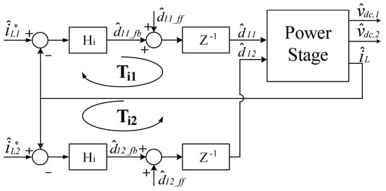
Figure 3.
Small signal current-loop control block diagram for grid current control.
2.3. Voltage Controller Design Method
It is necessary to design a voltage controller that can control input voltages of the PV arrays to determine the current reference in the state where the current controller is implemented. When the current-loops are closed, the transfer functions of the input voltages (Vdc,1, Vdc,2) to each H-bridge module current are firstly derived. Then, the voltage controller should be designed to stabilize the transfer function of the voltages to the current reference, and the detailed procedure is as follows.
The previously mentioned current loop closed system can be considered as the TITO system as shown in dotted box of Figure 4. g11 is the transfer function of the upper PV array voltage of the upper H-bridge module, with respect to the reference current, denoted as , and g12 is the transfer function of the upper PV array voltage of the lower H-bridge module, with respect to the reference current, denoted as . The derived transfer functions are represented as (14)–(17). In Figure 4, Hv represents the controller for the voltage control of the current loop closed system.
where Hi is the PI current controller and Ti1 and Ti2 are the current loop gains that are denoted as HiGiLd1 and HiGiLd2, respectively.
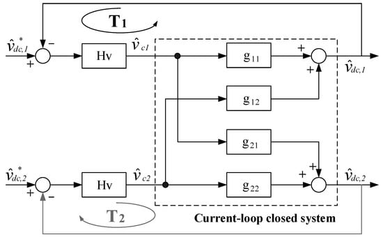
Figure 4.
Voltage control loop block diagram of current-loop closed plant system.
Similarly, g21 is the transfer function of the lower PV array voltage of the upper H-bridge module, with respect to the reference current, denoted as , and the g22 is the transfer function of the lower PV array voltage of the lower H-bridge module, with respect to the reference current, denoted as . The transfer functions are derived as (18)–(21).
Thus, the outer voltage control-loops are designed to stabilize the current-loop closed system using the following loop design approach. Voltage loop T1 is first designed without the voltage loop T2. In this condition, the transfer function of the control voltage Vc2 to DC voltage Vdc2 with the closed T1 loop can be derived as (22). In this equation, several loop gains are defined as follows:, , , and .
In this case, Hv is a voltage controller defined by (23), and DC gain and zero of the PI controller are designed so that the control loop T2 has the desired cutoff bandwidth and the phase margin. This sequential design approach can be used to achieve the control objectives and stability.
Because the system is a TITO system, the individual DC voltage control scheme has loop interaction. Thus, in order to minimize loop interaction, the inverted decoupling control scheme in Figure 5 can be employed.
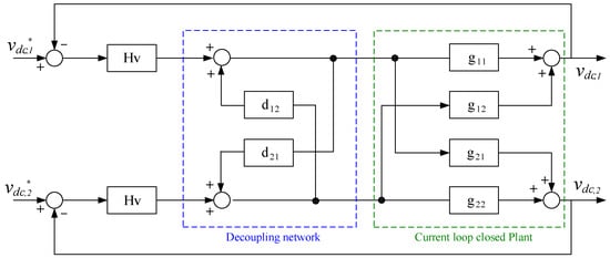
Figure 5.
Inverted decoupling method of two-input and two-output system.
The objective is to obtain the diagonal matrix in the series combination, between the matrix of the decoupling network and the matrix of the current-loop closed system [38]. In the inverted decoupling method, the off-diagonal elements are derived as (24) and (25).
3. Results
From the design point of view of the power converter, the single-phase grid-connected inverter should be able to operate at universal voltages up to 240 Vrms. If the output voltage of each H-bridge module is Vsw1 and Vsw2 in Figure 1, the current flowing in the system can be controlled by using the vector sum of the two output voltages as shown in Figure 6. Therefore, since the sum of the two output voltages must be greater than the grid voltage, the sum of the voltages of the two PV arrays must be set to 380 V or more. If the upper H bridge module is manufactured with a 300 V class power devices, the PV array can be designed to have a voltage of 200 V class. (5 series-configured arrays if the open-circuit voltage of the individual PV modules is 40 V). Since this paper focuses on the controller design of cascaded H-bridge inverter, we verify the performance based on the experimental set presented in Figure 7 and Table 1. In the experimental set, two isolated power supplies with series resistors for emulating PV arrays are used, as shown in Figure 7. Since the output characteristics of each PV array can be controlled, the performance of the controller can be verified using the unbalanced PV output case shown in Figure 8.
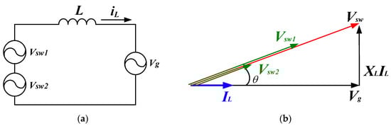
Figure 6.
AC-side equivalent circuit and the phasor diagram of H-bridge output voltages for the unity power factor. In figure, XL is the impedance of the output inductor, XL = ωL. (a) AC-side equivalent circuit, (b) phasor diagram of voltages and current for the unity power factor.
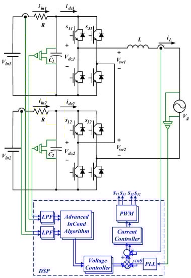
Figure 7.
Experimental hardware setup and control block diagram of the prototype cascaded H-bridge multilevel inverter system.

Table 1.
System parameters of the prototype PV system.
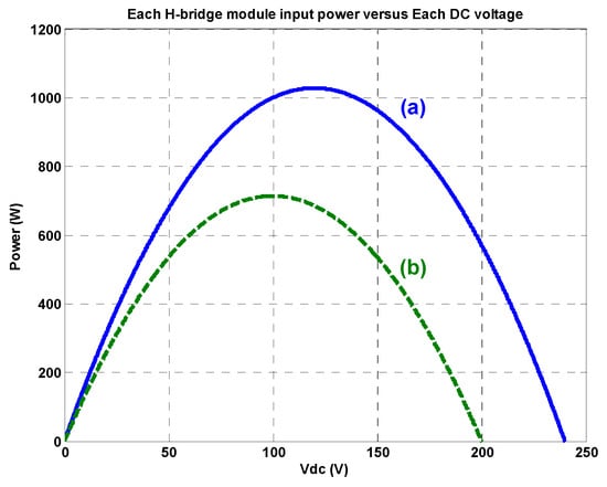
Figure 8.
Each input power versus each DC voltage characteristics. (a) emulated PV system with the maximum 1 kW at 240 V DC voltage, (b) emulated PV system with the maximum 714 W at 200 V DC voltage.
Two DC power supplies, having an operating voltage range of 0–250 V and two resistors (R1 and R2) of 14 Ω, are selected. In this condition, the voltage loop gain of the experimental system is shown in Figure 9. The cutoff frequency of the voltage loop gain is 30–40 Hz, and the phase margin is around 45° for both input conditions. The analysis results of the feedforward current controller designed in Section 2 are shown in Figure 10. When feedforward is applied, it can be seen that the effect of the grid voltage on the grid current is further attenuated by −30 dB at the grid voltage frequency of 60 Hz.
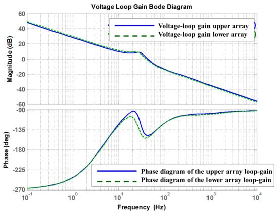
Figure 9.
Voltage loop gain bode diagram of cascaded multilevel inverter system; Blue solid line is a voltage loop-gain bode diagram of the upper H-bridge module and a green dotted line is a voltage loop-gain bode diagram of the lower H-bridge module.
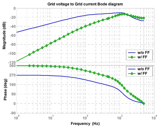
Figure 10.
Grid-voltage disturbance effects with and without the duty-ratio feed forward on the condition of the output voltage of the PV is 120 V and output power is 1 kW.
Figure 11 shows the simulation results of the control performance for the designed voltage controller in Figure 9. In order to demonstrate the validity of the voltage controller designed with a cutoff frequency of 30 Hz, we simulated whether the DC voltages of the upper and lower H-bridge modules were tracking the voltage reference of 120 + 5sin (2π × 3t) V and 120 + 5sin (2π × 30t) V. Figure 11a shows the voltage control result when 120 + 5sin (2π × 3t) V is input as the DC link voltage reference of the upper and lower H-bridge modules. It can be seen that the average DC voltage follows the voltage reference except 120 Hz DC voltage ripple due to the pulsating power of double frequency of the grid voltage frequency present in the instantaneous power of the single phase system [39]. Figure 11b shows DC voltage control results of the upper and lower H-bridge modules for 120 + 5 sin (2π × 30t) V voltage references. As in the previous case, it can be seen that the DC voltage can follow the DC input voltage command on average, although there is a 120 Hz voltage ripple. Figure 11c is the 1-period enlarged waveform from the result of (a). As shown in the bottom result, it can be confirmed that the current is controlled to be in phase with the grid voltage.
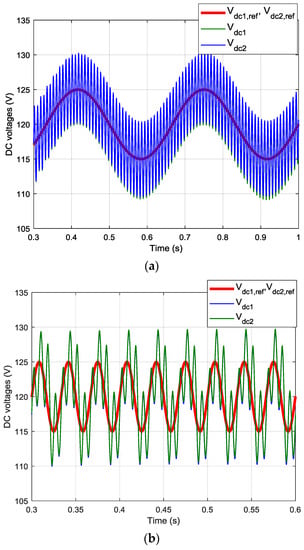
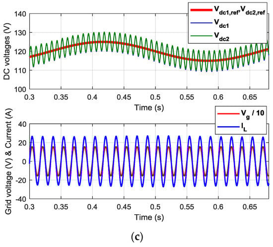
Figure 11.
Simulation results for DC voltage control of the upper and lower H-bridge modules for the DC link voltage reference including a sinusoidal voltage. (a) results for 120 + 5sin(2π × 3t) V voltage reference, (b) results for 120 + 5sin(2π × 30t) V voltage reference, (c) 1-period enlarged waveform of (a).
To verify the independent DC link voltage control of the cascaded H-bridge inverter, a simulation considering the voltage reference step change is conducted with the conditions shown in Figure 7 and Table 1. In Figure 12, the DC link voltages of two H-bridge modules are initially controlled at 120 V. After 0.5 s, the upper H-bridge module voltage reference is changed to 130 V, and the lower module reference is changed to 110 V. Without employing the decoupling scheme, we can see the oscillatory voltage waveforms in light blue and light green. This oscillatory response results in a reduction in the conversion efficiency, and increase the system instability. However, when applied to the decoupling method, the input voltages of the two PV arrays can be stably controlled to their reference value, as shown in the blue and green waveforms.
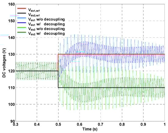
Figure 12.
Simulation result of the individual voltage control with respect to the step changes of the DC-input reference with (w/) and without (w/o) inverted decoupling control method.
Figure 13 and Figure 14 show the experimental results of an individual DC-link voltage and grid current control performance. Even though the two input source characteristics are different, maximum powers from each input source are extracted by controlling the individual DC voltage using the proposed method. In Figure 13, since the voltage of two input DC power sources is 240 V, the DC-link voltages at which maximum power is generated are 120 V. In Figure 14, because the two input DC supplies are 240 V and 200 V, the voltages of the maximum power are 120 V and 100 V, respectively. In the voltage control results shown in Figure 13, Figure 14 and Figure 15, the single-phase power injected into the grid includes the pulsating power with twice the frequency of the grid voltage as mentioned in reference [39]. However, it can be confirmed by the designed controller that the average voltage follows the voltage reference. In addition, the inverter output voltage of the cascaded H-bridge modules exhibits a five-level stair-case waveform. The grid current of Figure 15, which is the enlarged waveform of Figure 13, is controlled in phase with the grid voltage, and the summed power is stably transferred to the utility grid.
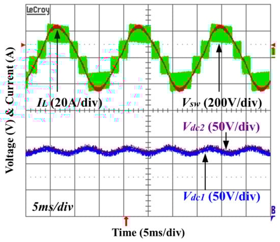
Figure 13.
Experimental results of DC link voltage and grid current control when the MPP voltage of upper H-bridge module and lower H-bridge module are 120 V respectively.
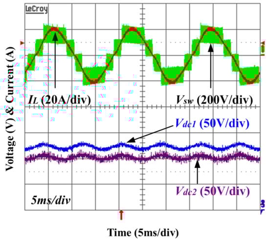
Figure 14.
Experimental results of DC link voltage and grid current control when the MPP voltage of upper H-bridge module and lower H-bridge module are 120 and 100 V respectively.
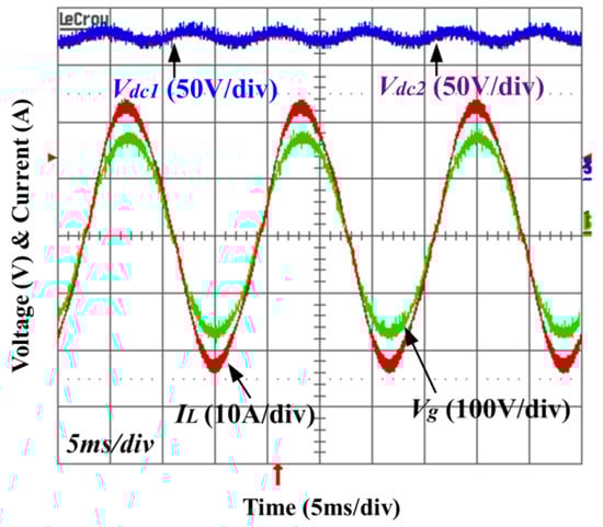
Figure 15.
Enlarged experimental results of Figure 13.
In this work, the DC voltage references are independently obtained from an advanced incremental conductance MPPT algorithm [40]. The algorithm flow-chart of the MPPT is shown in Figure 16. The variable DC step size is defined as (26) and is determined using the relationship of the incremental and instantaneous resistance of the PV arrays. The update period of the MPPT algorithm is set to 2 s and the maximum step size for changing the voltage references is 5 V.
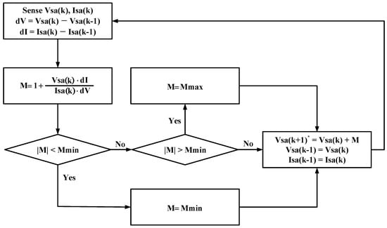
Figure 16.
Algorithm flow-chart of the advanced incremental conductance method.
Figure 17 shows the MPPT performance. Initially, because the power conversion system (PCS) does not work, the output DC voltages of the PV arrays are 240 V. After starting the operation, both output DC voltages of the PV arrays are controlled to their maximum power points. Further, the generated power of the PV arrays is transferred to the utility grid as shown in the red waveform.
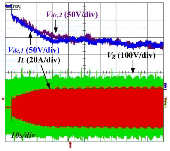
Figure 17.
Experimental results for maximum power point tracking.
4. Conclusions
In this paper, the modeling and controller design methods for individual MPPT of the single-phase cascaded H-bridge multilevel PV inverter are proposed. The small signal transfer functions are derived through the small-signal modeling approach. For the unity power factor, a PI current controller with a duty ratio feed-forward compensation method is employed. In order to achieve the individual MPPT of the PV arrays, each of the DC link voltage loops is designed to stabilize the current loop closed system. Especially, in order to avoid loop interaction in the current loop closed system, the voltage controller design with the inverted decoupling method is proposed. The inverted decoupling method to minimize the loop interaction of the TITO system has been verified by the simulation result, but the experimental performance will be done through the future work. The proposed control methods of the cascaded H-bridge multilevel PV inverter are validated through the simulation and experimental results on the 2-kW prototype system.
Author Contributions
S.L. contributed to the main idea of this article, and wrote the paper. S.L. and J.K. performed the experiments. J.K. revised the paper critically. All authors approved the final version to be published.
Acknowledgments
This research was supported by Program through the National Research Foundation of Korea (NRF) funded by the Ministry of Science and ICT (NO.NRF-2017M1A3A3A06016680, Cubesat Contest and Development) and funded by the Hanwha Land Systems.
Conflicts of Interest
The authors declare no conflict of interest.
References
- Rodriguez, J.; Lai, J.-S.; Peng, F.Z. Multilevel inverters: A survey of topologies, controls, and applications. IEEE Trans. Ind. Electron. 2002, 49, 724–738. [Google Scholar] [CrossRef]
- Lai, J.-S.; Peng, F.Z. Multilevel converters-A new breed of power converters. IEEE Trans. Ind. App. 1996, 32, 509–517. [Google Scholar] [CrossRef]
- Selvaraj, J.; Rahim, N.A. Multilevel inverter for grid-connected PV system employing digital PI controller. IEEE Trans. Ind. Electron. 2009, 56, 149–158. [Google Scholar] [CrossRef]
- Vilanueva, E.; Correa, P.; Rodriguez, J.; Pacas, M. Control of a single-phase cascaded H-bridge multilevel inverter for grid-connected photovoltaic systems. IEEE Trans. Ind. Electron. 2009, 56, 4399–4406. [Google Scholar] [CrossRef]
- Zabihinejad, A.; Viarouge, P. Mass minimization and sensitivity analysis of high power modular multilevel converter. Int. J. Electr. Power Energy Syst. 2017, 93, 328–339. [Google Scholar] [CrossRef]
- Shekhar, A.; Kontos, E.; Ramirez-Elizondo, L.; Rodrigo-Mor, A.; Bauer, P. Grid capacity and efficiency enhancement by operating medium voltage AC cables as DC links with modular multilevel converters. Int. J. Electr. Power Energy Syst. 2017, 93, 479–493. [Google Scholar] [CrossRef]
- Hasan, N.S.; Rosmin, N.; Osman, D.A.A.; Musta’amal, A.H. Reviews on multilevel converter and modulation techniques. Renew. Sustain. Energy Rev. 2017, 80, 163–174. [Google Scholar] [CrossRef]
- Gupta, A. Influence of solar photovoltaic array on operation of grid-interactive fifteen-level modular multilevel converter with emphasis on power quality. Renew. Sustain. Energy Rev. 2017, 76, 1053–1065. [Google Scholar] [CrossRef]
- Lee, S.S.; Heng, Y.E. A voltage level based predictive direct power control for modular multilevel converter. Electr. Power Syst. Res. 2017, 148, 97–107. [Google Scholar] [CrossRef]
- Guo, J.; Jiang, D.; Zhou, Y.; Hu, P.; Lin, Z.; Liang, Y. Energy storable VSC-HVDC system based on modular multilevel converter. Int. J. Electr. Power Energy Syst. 2016, 78, 269–276. [Google Scholar] [CrossRef]
- Iman-Eini, H.; Schanen, J.-K.; Farhangi, S.H.; Wang, S. Design of cascaded H-bridge rectifier for medium voltage applications. In Proceedings of the IEEE Power Electronics Specialist Conference, Orlando, FL, USA, 17–21 June 2007; pp. 653–658. [Google Scholar] [CrossRef]
- Daher, S.; Schmid, J.; Antunes, F.L.M. Multilevel inverter topologies for stand-alone PV systems. IEEE Trans. Ind. Electron. 2008, 55, 2703–2712. [Google Scholar] [CrossRef]
- Iman-Eini, H.; Farhangi, S.; Khakbazen-Fard, M.; Schanen, J.-L. Analysis and control of a modular MV-to-LV rectifier based on a cascaded multilevel converter. J. Power Electron. 2009, 9, 133–145. [Google Scholar]
- Zhang, Y.; Ravishankar, J.; Fletcher, J.; Li, R.; Han, M. Review of modular converter based multi-terminal HVDC systems for offshore wind power transmission. Renew. Sustain. Energy Rev. 2016, 61, 572–586. [Google Scholar] [CrossRef]
- António-Ferreira, A.; Gomis-Bellmunt, O. Modular multilevel converter losses model of HVdc applications. Electr. Power Syst. Res. 2017, 146, 80–94. [Google Scholar] [CrossRef]
- Xiao, B.; Filho, F.; Tolbert, L. Single-phase cascaded H-bridge multilevel inverter with nonactive power compensation for grid-connected photovoltaic generators. In Proceedings of the IEEE Energy Conversion Congress and Exposition, Phoenix, AZ, USA, 17–22 September 2011; pp. 2733–2737. [Google Scholar]
- Verma, V.; Kumar, A. Single phase cascaded multilevel photovoltaic sources for power balanced operation. In Proceedings of the IEEE 5th India International Conference on Power Electronics (IICPE), Delhi, India, 6–8 December 2012; pp. 1–6. [Google Scholar] [CrossRef]
- Calais, M.; Agelidis, V.G.; Borle, L.J.; Dymond, M.S. A transformerless five level cascaded inverter based single phase photovoltaic system. In Proceedings of the IEEE 31th Annual Power Electronics Specialist Conference, Galway, Ireland, 23 June 2000; pp. 1173–1178. [Google Scholar]
- González, M.; Cárdenas, V.; Miranda, H.; Álvarez-Salas, R. Conception of a modular multilevel converter for high-scale photovoltaic generation based on efficiency criteria. Sol. Energy 2016, 125, 381–397. [Google Scholar] [CrossRef]
- Fuentes, C.D.; Rojas, C.A.; Renaudineau, H.; Kouro, S.; Perez, M.A.; Meynard, T. Experimental validation of a single DC bus cascaded H-bridge multilevel inverter for multistring photovoltaic systems. IEEE Trans. Ind. Electron. 2017, 64, 930–934. [Google Scholar] [CrossRef]
- Yu, Y.; Konstantinou, G.; Hredzak, B.; Agelidis, V.G. Power balance of cascaded H-bridge multilevel converters for large-scale photovoltaic integration. IEEE Trans. Power Electron. 2016, 31, 292–303. [Google Scholar] [CrossRef]
- Farivar, G.; Hredzak, B.; Agelidis, V.G. A DC-side sensorless cascaded H-bridge multilevel converter-based photovoltaic system. IEEE Trans. Ind. Electron. 2016, 63, 4233–4241. [Google Scholar] [CrossRef]
- Yu, Y.; Konstantinou, G.; Townsend, C.D.; Agelidis, V.G. Comparison of zero-sequence injection methods in cascaded H-bridge multilevel converters for large-scale photovoltaic integration. IET Renew. Power Gener. 2017, 11, 603–613. [Google Scholar] [CrossRef]
- Letha, S.S.; Thakur, T.; Kumar, J. Harmonic elimination of a photo-voltaic based cascaded H-bridge multilevel inverter using PSO (particle swarm optimization) for induction motor drive. Energy 2016, 107, 335–346. [Google Scholar] [CrossRef]
- Sastry, J.; Bakas, P.; Kim, H.; Wang, L.; Marinopoulos, A. Evaluation of cascaded H—bridge inverter for utility-scale photovoltaic systems. Renew. Energy 2014, 69, 208–218. [Google Scholar] [CrossRef]
- Mao, M.; Zhang, L.; Duan, Q.; Chong, B. Multilevel DC-link converter photovoltaic system with modified PSO based on maximum power point tracking. Sol. Energy 2017, 153, 329–342. [Google Scholar] [CrossRef]
- Boukenoui, R.; Ghanes, M.; Barbot, J.-P.; Bradia, R.; Mellit, A.; Salhi, H. Experimental assessment of maximum power point tracking methods for photovoltaic systems. Energy 2017, 132, 324–340. [Google Scholar] [CrossRef]
- Ram, J.P.; Rajasekar, N.; Miyatake, M. Design and overview of maximum power point tracking techniques in wind and solar photovoltaic systems: A review. Renew. Sustain. Energy Rev. 2017, 73, 1138–1159. [Google Scholar] [CrossRef]
- Kermadi, M.; Berkouk, E.M. Artificial intelligence-based maximum power point tracking controllers for photovoltaic systems: Comparative study. Renew. Sustain. Energy Rev. 2017, 69, 369–386. [Google Scholar] [CrossRef]
- Zhao, J.; Zhou, X.; Gao, Z.; Ma, Y.; Qin, Z. A novel global maximum power point tracking strategy (GMPPT) based on optimal current control for photovoltaic systems adaptive to variable environmental and partial shading conditions. Sol. Energy 2017, 144, 767–779. [Google Scholar] [CrossRef]
- Fathabadi, H. Novel fast and high accuracy maximum power point tracking method for hybrid photovoltaic/fuel cell energy conversion systems. Renew. Energy 2017, 106, 232–242. [Google Scholar] [CrossRef]
- Docimo, D.J.; Ghanaatpishe, M.; Mamun, A. Extended Kalman Filtering to estimate temperature and irradiation for maximum power point tracking of a photovoltaic module. Energy 2017, 120, 47–57. [Google Scholar] [CrossRef]
- Ram, J.P.; Rajasekar, N. A new global maximum power point tracking technique for solar photovoltaic (PV) system under partial shading conditions (PSC). Energy 2017, 118, 512–525. [Google Scholar] [CrossRef]
- Alonso, O.; Sanchis, P.; Gubia, E.; Marroyo, L. Cascaded H-bridge multilevel converter for grid connected photovoltaic generators with independent maximum power point tracking of each solar array. In Proceedings of the IEEE 34th Annual Conference on Power Electronics Specialist, Acapulco, Mexico, 15–19 June 2003; pp. 731–735. [Google Scholar]
- Lee, S.J.; Bae, H.S.; Cho, B.H. Modeling and control of the single-phase photovoltaic grid-connected cascaded H-bridge multilevel inverter. In Proceedings of the IEEE Energy Conversion Congress and Exposition, San Jose, CA, USA, 20–24 September 2009; pp. 43–47. [Google Scholar] [CrossRef]
- Polivka, W.M.; Chetty, P.R.K.; Middlebrook, R.D. State-space average modeling of converters with parasitic and storage-time modulation. In Proceedings of the IEEE Power Electronics Specialist Conference, Atlanta, Georgia, USA, 16–20 June 1980; pp. 119–143. [Google Scholar] [CrossRef]
- Kazimierczuk, M.K. Pulse-Width Modulated DC-DC Power Converters; Wiley: Hoboken, NJ, USA, 2008. [Google Scholar]
- Gagnon, E.; Pomerleau, A.; Desbiens, A. Simplified, ideal or inverted decoupling. ISA Trans. 1998, 37, 265–276. [Google Scholar] [CrossRef]
- Chen, Y.; Chang, C.; Wu, H. DC-link capacitor selections for the single-phase grid-connected PV system. In Proceedings of the 2009 International Conference on Power Electronics and Drive Systems (PEDS), Taipei, Taiwan, 2–5 November 2009; pp. 72–77. [Google Scholar] [CrossRef]
- Lee, J.H.; Bae, H.; Cho, B.H. Advanced incremental conductance MPPT algorithm with a variable step size. In Proceedings of the 12th International Power Electronics and Motion Control Conference, Portoroz, Slovenia, 30 August–1 September 2006; pp. 603–607. [Google Scholar]
© 2018 by the authors. Licensee MDPI, Basel, Switzerland. This article is an open access article distributed under the terms and conditions of the Creative Commons Attribution (CC BY) license (http://creativecommons.org/licenses/by/4.0/).