Precision Modeling: Application of Metaheuristics on Current–Voltage Curves of Superconducting Films

Abstract

Contemplating the importance of studying current–voltage curves in superconductivity, it has been recently and rightly argued that their approximation, rather than incessant measurements, seems to be a more viable option. This especially becomes bona fide when the latter needs to be recorded for a wide range of critical parameters including temperature and magnetic field, thereby becoming a tedious monotonous procedure. Artificial neural networks have been recently put forth as one methodology for approximating these so-called electrical measurements for various geometries of antidots on a superconducting thin film. In this work, we demonstrate that the prediction accuracy, in terms of mean-squared error, achieved by artificial neural networks is rather constrained, and, due to their immense credence on randomly generated networks’ coefficients, they may result in vastly varying prediction accuracies for different geometries, experimental conditions, and their own tunable parameters. This inconsistency in prediction accuracies is resolved by controlling the uncertainty in networks’ initialization and coefficients’ generation by means of a novel entropy based genetic algorithm. The proposed method helps in achieving a substantial improvement and consistency in the prediction accuracy of current–voltage curves in comparison to existing works, and is amenable to various geometries of antidots, including rectangular, square, honeycomb, and kagome, on a superconducting thin film.

1. Introduction

Precisely measuring critical current density in superconducting materials and systems requires understanding of the fundamentals of current–voltage (IV) characteristics, also called the transport measurements [1]. Recent studies have shown that these IV curves may show sudden jumps, which resemble Shapiro steps, in voltage around critical current ($I_c$) and/or critical temperature ($T_c$) in superconducting thin films. These steps usually appear when the vortex lattice is formed, which may lead to instability at high vortex velocities. These instabilities have been studied in different systems including nanotube Josephson Junctions [2], superconducting nanowires [3], low temperature thin films [4], and a square array of periodic antidots on an Nb film [5]. Studying such behavior in superconducting films is important since Shapiro steps are exploited to make flux Qubits that are essential for superconducting quantum computers [6]. Other mechanisms that may lead to such jumps include thermo-magnetic instabilities of vortex matter [7], thermally-assited flux flow [8], or just overheating of the superconducting film on SiO${}_2$ substrate.

Fabrication of various geometries by electron-beam lithography, to obtain transport measurements via a physical properties measurement system (PPMS), is an expensive, tedious and cumbersome process [9]. It has been recently pointed out that these curves, especially when they are needed for a wide range of temperature and magnetic field values, may not be necessarily measured incessantly; instead, they may be obtained using some approximation technique applied on a finite amount of curves already obtained via PPMS [10,11,12]. Artificial Neural Networks (ANN) have been used as the approximation method in each of these solutions to extrapolate the IV curves for unforeseen values of critical parameters. It shall be discussed in Section 2.2 that training the ANN requires two randomly generated networks’ coefficients called weights and biases, which are updated in each iteration, until an optimal solution (with the smallest mean-squared error, MSE) is obtained. Mainly due to this randomness in the coefficient generation, ANN tends to converge to one local minima from a pool of possible solutions, which makes training of the ANN a nondeterministic process. The latter, in turn, may lead to inordinately varying values of MSE, number of iterations, and time to converge. In this way, two rounds of training on the same data may result in different prediction accuracies.

The proposed work intends to address the aforesaid problem by controlling the randomness in coefficient generation, such that the ANN always converges (close) to the global minima, by means of a novel entropy based genetic algorithm. Our case study is the prediction of IV curves for four different geometries of antidots, including rectangular, square, honeycomb, and kagome, on an Nb film. However, the proposed approach is equally applicable to other superconducting films as an alternative approximation technique for measuring other properties at the same time. The main contribution of the proposed work, therefore, is the increased accuracy in the prediction of IV curves by means of Entropy, which in a nutshell is the uncertainty measurement associated with initialization of the weights and biases. Since ANN are highly dependent on their initial conditions for their fast convergence and accurate approximation, the selected vector of weights and biases should have a minimum entropy. To the best of our knowledge, entropy, especially in conjunction with genetic algorithm (GA), has never been adopted for the prediction of IV curves for a superconducting film, which, we show, outperforms the conventionally used predictors.

The rest of the paper is organized as following: Section 2 covers our experimental setup and a brief overview of existing methodologies and relevant works. We present the problem formulation in Section 3. Section 4 presents the proposed methodology, and an overview of GA. In Section 5, we present simulation results and a comparative analysis of the used algorithms, before we conclude the paper in Section 6.

2. Related Work and Experimental Setup

In order to be able to draw a fair comparison between the proposed methodology and the existing works, we decided to adopt the same experimental setup and the superconducting film of the same thickness. In what follows, we give an overview of the experimental setup and fundamentals of the ANN, which is mainly an extract of the benchmark works [10,11,12].

2.1. Experimental Setup and Measurements Using PPMS

For our experiments, we deposited a high quality 60 nm Nb film on a SiO${}_2$ substrate, followed by fabrication of micro-bridges by ultraviolet photolithography and dry etching in order to obtain transport measurements. The desired geometries of circular antidots were obtained by applying e-beam lithography on a photo-resist layer. Finally, magnetically enhanced dry etching transferred the patterns to the film. A commercially available PPMS was used to perform the transport measurements. Figure 1 presents the scanning electron microscopy (SEM) of various geometries.

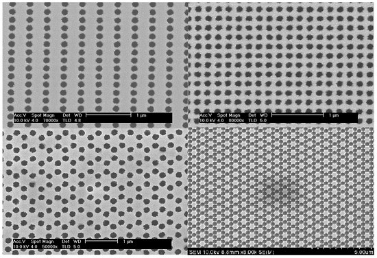
Figure 1. Scanning Electron Micrograph of superconducting Nb film with four geometries: top left-right (rectangular-square), bottom left-right (honeycomb-kagome).

In the IV curves measured at different values of temperature and magnetic field, shown in Figure 2, we observed Shapiro steps around $T_c$. However, these steps continued to weaken with increasing temperature until it completely vanished. These temperature dependent curves might be divided into three regions: between two regions—in each of which the curve showed some slope—there was a region that comprised the Shapiro steps. We repeatedly varied magnetic fields and kept the current constant, and vice versa to collect 25,600 samples arranged in a 4 $\times$ 4 $\times$ 1600 matrix for each geometry, where 4 $\times$ 4 refers to the 4 constant values of current and magnetic fields. In our proposed work, we isolated one sample from each matrix and subjected the rest for training the ANN model. Once trained, the isolated sample should be compared with the predicted curve for the same values of magnetic field and temperature.

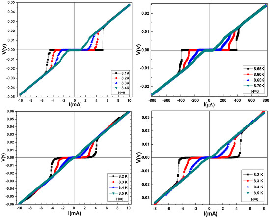
Figure 2. The IV characteristics of four geometries at different temperatures and magnetic fields: top left-right (rectangular-square), bottom left-right (honeycomb-kagome).

2.2. Approximation Using ANN

ANN imitate a human brain and are supposed to perform learning in a given situation and repeat in another [13]. They tend to establish relationships between independent variables of a small subset, and are widely used for approximation on a larger sample space by utilizing those relationships. An ANN architecture, mainly, is an interconnection of several neurons [14] in a directed graph, which provide mapping from an input layer to an output layer via a few hidden layers sandwiched in between. The neurons in each layer carry some real weights and bias—together called networks’ coefficients. A different set of weights, which are updated in each iteration of the training process, leads to a different network’s response. A number of training algorithms exist in literature—each of which updates the coefficients in a unique manner, but, for most of them backpropagate, their errors from the output layer to input layer in order to minimize the objective function. The goal of this training or learning process is to achieve the smallest mean squared error (MSE) between the target and the actual system’s response [15]. The network’s response carrying only one hidden layer is given by Equation (1):

$$y_k={\delta }_o(\sum _{j=0}^M{w}_{kj}^y({\delta }_H(\sum _{i=0}^N{w}_{ji}^H{x}_i+b_i))+b_j),$$

(1)

where ${\delta }_o$ and ${\delta }_H$ are the threshold or activation function in the output and hidden layer, respectively, w and b represent weights and bias terms, respectively, and $x_i$ represents the ith element in the input layer.

Without going into details of the available training algorithms, in this work, we will stick only to those that were used for the same purpose in the benchmark works. The first work [12] that proposed to approximate the IV curves for an Nb film made use of Bayesian Regularization (BR) algorithm for training the ANN for a square array of antidots. The algorithm converged in fifty-five iterations (epochs), and managed to achieve the best MSE of $2.08\times {10}^{-8}$. This work did not explore other available options—be it in terms of training algorithms or ANN architectures.

The second benchmark work [10] in contrast did the same for a diluted square lattice and presented a thorough comparison between three different ANN architectures, each with ten different configurations (number of neurons in each layer), and trained by six training algorithms—a total of 180 ANN models were developed, and the best MSE obtained was $4.55\times {10}^{-8}$. Figure 3 shows the MSE obtained by all the models, where cascaded, feedforward, and layer recurrent are the three ANN architectures; it is important to note the diversity in the obtained results, which is mainly due to random nature of the generated coefficients.

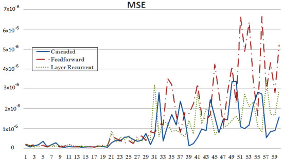
Figure 3. MSE achieved by a benchmark work for three ANN architectures. Reprinted from [10] with permission.

The last benchmark work [11] was an extension of the second benchmark, in which a comparison was drawn between four geometries of antidots on the same Nb film. The lowest MSB reported in this work was in the order of $\times {10}^{-9}$ for a specific architecture and a specific training algorithm. However, the diversity in the obtained results was once again enormous, and nondeterministic.

Other than these benchmark works, there have been a few notable attempts on proposing formal models for analyzing IV curves for superconducting devices and films. For instance, a formal, self-consistent, model was presented for estimating critical current of superconducting devices [16]. The authors admitted that an array of antidots based thin film was very difficult to model mathematically. Although its computation burden was less than that of the ANN based models, it lacked accuracy—tolerance of 4–6% within actual values as compared to the ANN models having tolerance less than 1% with the actual values. Another attempt based on ANN was presented by Bonanno et al. [17]. The authors proposed a radial basis function neural network (RBFNN) and demonstrated that it had a prediction accuracy of about ${10}^{-1}$ (MSE), which is even lesser than the already existing techniques—let alone our current model based on a genetic algorithm, achieving MSE in the order of ${10}^{-9}$.

3. Problem Statement

Let $\mathsf{\Omega }\subset {\mathbb{R}}^{\nu }$, where $\nu =2;\nu \to$ {$R^{\prime }\times D^{\prime }$}$|R^{\prime }>D^{\prime }$, be an experimental values. Let the selected feature set, $\varphi =\varphi \left(i\right)|i\in \mathsf{\Omega }$ where ${\varphi }_1\left(i\right),\dots ,{\varphi }_n\left(i\right)\subset \varphi$ are associated with the ANN training process to predict output vector ${\tilde{\varphi }}_{pred}$. The set of features $\varphi$ are mapped to ${\tilde{\varphi }}_{pred}$: $\varphi \to {\tilde{\varphi }}_{pred}$. The output vector ${\tilde{\varphi }}_{pred}$ is calculated as:

$$\{{\tilde{\varphi }}_{pred}\stackrel{\Delta }{=}({\delta }_{WB}^k,po{p}_t,{\delta }_R,{\delta }_s)\in \{-1:1\},({\delta }_E^k,{\delta }_{WB}^{\prime },X_{ofs}^{\prime },{\varphi }_{pred}^y)\in {\mathbb{R}}^2\},$$

where the set of variables ${\delta }_{WB}^k$, $po{p}_t$, ${\delta }_R$, ${\delta }_s$, ${\delta }_E^k$, $X_{ofs}^{\prime }$ and ${\varphi }_{pred}^y$ have been described in the list of symbols. The objective function in case of ANN is selected to be MSE given in the following relation:

$$\mathsf{\Gamma }\left(\tilde{w}\right)=\mathsf{\Psi }\sum _{q=1}^Q{({\mathsf{\Gamma }}_{tar}-{\mathsf{\Gamma }}_{act})}^T({\mathsf{\Gamma }}_{tar}-{\mathsf{\Gamma }}_{act})=\mathsf{\Psi }\sum _{q=1}^Q{e}_q^2.$$

(2)

4. Proposed Optimization of ANN’s Coefficients

4.1. Genetic Algorithms

Genetic Algorithm (GA) is an evolutionary technique belonging to a class of stochastic search algorithms, which finds an optimal solution from a pool of solutions based on the principle of survival of the fittest [18]. In GA framework, each individual is represented by a string called a chromosome, whereas a group of chromosomes generate a population. For this architecture, weights and biases vector (chromosome) is generated, which is replicated multiple times to generate a population of some pre-defined size.

Binary representation of a GA is commonly used where each chromosome is a vector c, constituting a set of m genes from the set $0,1$:

$$C_i^k=\{G_1^k,G_2^k,\dots ,G_m^k\}{G}_m^k\in \{0,1\},$$

where m is the length of a chromosome.

However, in practical optimization, it is more natural to represent a gene in real numbers for an optimized solution [19]. The continuous domain provides larger space and more convergence possibilities. Data range is normalized to the range of $0⟶1$ prior to binary encoding, and, for this specific application, the chromosome is a floating point vector. In what follows, we present a few GA operators, called crossover and mutation, implemented for a thorough technical analysis.

4.1.1. Crossover Operators

Selecting a pair of chromosome $C_i^1=(G_1^1,G_2^1,\dots ,G_m^1)$ and $C_i^2=(G_1^2$, $G_2^2$, $\dots$, $G_m^2)$ for a multiple crossover description.

• Flat Crossover
  An offspring $O^i$ is generated where $O_i^k=(g_1^k,g_2^k,\dots ,g_m^k)$ is a uniformly chosen random value from the interval $[min(G_i^1,G_i^2),max(G_i^1,G_i^2)],$
  where m is the index for the number of genes and k is the index for the number of chromosomes.
• Linear Breeder Genetic Algorithm (BGA) Crossover
  Under the same consideration as above, let $O_i=G_1^1\pm ran{g}_i.\gamma .\Lambda$, where $\Lambda =(G_i^2-G_i^1)/\Vert G^1-G^2\Vert$ and $\gamma ={\sum }_{l=0}^{15}{\alpha }_l{2}^{-l}$. An $\alpha \in \{0,1\}$ is generated randomly with the probability of $p({\alpha }_i=1)=1/12$. Usually, $ran{g}_i=0.5({\kappa }_i-{\tau }_i)$ and − sign is chosen with the probability of 0.8 [20].
• Arithmetic Crossover
  In arithmetic crossover, two Offsprings are generated, $O^k=(g_1^k,g_2^k,\dots ,g_m^k)$, $k=1,2$ where: $g_i^1=\lambda G_i^1+(1-\lambda )G_i^2$ and $g_i^2=\lambda G_i^2+(1-\lambda )G_i^1$. Here, $\lambda$ is a constant and user-defined value, which can vary with the number of generations.

4.1.2. Mutation Operator

Let the maximum number of generations be represented by $R_{max}$ and $R_t$ denotes the generation on which mutation operator is applied. As per mutation rule:

$$G_i^{\prime }=\left\{\begin{array}{cc}{G}_i+\delta (t,{\kappa }_i-G_i),\hfill & \mathrm{if}\gamma =0,\hfill \\ G_i+\delta (t,G_i-{\tau }_i),\hfill & \mathrm{if}\gamma =1.\hfill \end{array}\right.$$

4.1.3. Selection

Selection is a process of selecting chromosomes with the smallest value of the cost function. The selection rate ${\varsigma }_{rate}$ defines the survivors eligible for mating in the next generation. Generally, the ${\varsigma }_{rate}$ = 50%, and the population selection is defined as:

$${\eta }_{rem}={\varsigma }_{rate}\times {\eta }_{pop},$$

(3)

$${\eta }_{keep}={\eta }_{pop}-{\eta }_{rem}.$$

(4)

The selection probability depends on the cost weight, calculated as:

$$P_k=\frac{C^k}{{\sum }_{j=1}^{{\eta }_{keep}}{C}^j}.$$

(5)

The chromosome with the lowest cost in terms of mean squared error has the highest selection probability. The other selection methods include roulette wheel, rank selection and tournament [21]. Roulette wheel is a probability based method, whereas the tournament selection is a winner-takes-all based technique [22].

4.1.4. Operation of a GA

The operation of a GA is summarized as follows:

• Create an initial population from a randomly generated weights and biases vector.
• Repeat until the best individuals are selected:
  • Evaluate the fitness using MSE,
  • Select the parents with best fitness level,
  • Apply the selected crossover and mutation operators.
• Terminate upon convergence.

Optimization is a process of finding the best possible solution from a given search space. In this work, an evolutionary strategy is utilized to fine-tune the parameters so as to minimize the cost function. Considering the GA’s exquisite performance on various platforms, and their ability to handle larger space problems even for stochastic objective functions, another domain is exploited, which is to optimize the solutions of artificial neural networks. The procedure has two possible directions: (1) optimize the weights and biases; and (2) optimize the architecture of ANN. In this work, the former method is used to improve the prediction accuracy.

4.2. Entropy Based GA for Optimization

For a set of discrete random variables $C_i^k=\{G_1^k,G_2^k,\dots ,G_m^k\}$, the Shannon entropy is defined as the following:

$${\delta }_E=-\sum _{k=0}^{m-1}(G_i^0/\delta G)lo{g}_2(G_i^0/\delta G),$$

(6)

$$\delta G=\sum _{k=0}^{m-1}{G}_0^i,$$

(7)

where $G_i^j$ is a vector of weights and biases called a chromosome.

The proposed cascaded design is the conjunction of three separate modules comprising an entropy calculator, GA optimizer, and ANN’s approximator. Here, the entropy calculator controls the uncertainty with the constraint of minimum randomness. The resulting vector, which is then forwarded to the GA module for optimization, comprises weights and biases with either minimum entropy or maximum repetition. Finally, the third module uses the optimized weights and biases to train the ANN for final approximation. Figure 4 summarizes the proposed methodology, and therefore the major contribution of this work, in a flow chart, and the proposed curve approximation with the optimized coefficients approach is given in Algorithm 1.

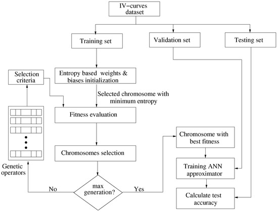
Figure 4. Flow chart depicting the proposed methodology.

Algorithm 1: Entropy based GA for weights and biases optimization

5. Simulation Results

5.1. Design Parameters

The number of hidden layers is fixed at three, where each has 27, 17, and 8 neurons in order; this is generally represented by network’s configuration {27 17 8}. The mutation rate is defined to be 0.2 and entropy count variable $\kappa$ is selected to be 200 for the optimal solution. Maximum generations of GA and maximum epochs of ANN are fixed to be 1000, while GA tolerance value $ϵ$ is selected to be $1\times {10}^{-8}$. Learning rate ${\delta }_r$ and initial step size ${\delta }_s$ are selected to be 0.9 and 0.8, respectively.

5.2. Results and Discussion

Table 1 explains the numerical comparisons of five different training algorithms which include Levenberg–Marquardt (LM), three variants of Conjugate Gradient (CG), and Bayesian, utilizing three crossover techniques for GA over four different geometries. It can be clearly observed, linear-BGA crossover technique in conjunction with Bayesian regularization framework outperforms other methods in terms of minimum epochs and MSE for all geometries. For the mentioned sequence (Linear-BGA + Bayesian Regularization), epochs are in the range of (36–47), whilst minimum MSE achieved is in the range of $(6.89\times {10}^{-9}$–$8.87\times {10}^{-9})$. The worst performance with linear-BGA is of CGP backpropagation having epochs in the range of 164–394. Similarly, with other crossover techinques, still Bayesian backpropagation acheives minimum MSE and also minimum epochs.

Table 1. Comparison of ANN’s training algorithms with multiple GA operators.

Algo.	Crossover	Epochs	MSE	Crossover	Epochs	MSE	Crossover	Epochs	MSE
LM	Flat	89	5.87 $\times {10}^{-7}$	Linear-BGA	17	3.55 $\times {10}^{-8}$	Arithmetic	136	5.87 $\times {10}^{-7}$
CGF		205	4.41 $\times {10}^{-7}$		292	3.16 $\times {10}^{-8}$		181	3.42 $\times {10}^{-7}$
CGB		784	2.12 $\times {10}^{-7}$		210	4.79 $\times {10}^{-8}$		331	9.80 $\times {10}^{-7}$
CGP		93	2.60 $\times {10}^{-7}$		394	6.08 $\times {10}^{-8}$		139	4.41 $\times {10}^{-7}$
Bayesian		49	5.84 $\times {10}^{-8}$		42	7.50 $\times {10}^{-9}$		107	6.24 $\times {10}^{-8}$
(a) Square Lattice
LM	Flat	79	4.11 $\times {10}^{-7}$	Linear-BGA	39	2.67 $\times {10}^{-8}$	Arithmetic	101	3.24 $\times {10}^{-7}$
CGF		190	4.20 $\times {10}^{-7}$		179	4.66 $\times {10}^{-8}$		199	2.79 $\times {10}^{-7}$
CGB		650	3.47 $\times {10}^{-7}$		265	5.61 $\times {10}^{-8}$		387	6.91 $\times {10}^{-7}$
CGP		110	1.97 $\times {10}^{-7}$		164	7.21 $\times {10}^{-8}$		170	5.76 $\times {10}^{-7}$
Bayesian		59	4.37 $\times {10}^{-8}$		47	6.89 $\times {10}^{-9}$		83	1.90 $\times {10}^{-8}$
(b) Rectangular Lattice
LM	Flat	94	4.74 $\times {10}^{-7}$	Linear-BGA	25	3.21 $\times {10}^{-8}$	Arithmetic	121	4.33 $\times {10}^{-7}$
CGF		220	4.78 $\times {10}^{-7}$		193	4.61 $\times {10}^{-8}$		174	2.90 $\times {10}^{-7}$
CGB		694	2.76 $\times {10}^{-7}$		235	4.71 $\times {10}^{-8}$		357	7.21 $\times {10}^{-7}$
CGP		101	1.34 $\times {10}^{-7}$		271	6.37 $\times {10}^{-8}$		157	4.99 $\times {10}^{-7}$
Bayesian		62	4.76 $\times {10}^{-8}$		41	7.10 $\times {10}^{-9}$		91	3.56 $\times {10}^{-8}$
(c) Honeycomb Lattice
LM	Flat	87	5.11 $\times {10}^{-7}$	Linear-BGA	31	3.66 $\times {10}^{-8}$	Arithmetic	132	5.81 $\times {10}^{-7}$
CGF		187	4.36 $\times {10}^{-7}$		216	4.12 $\times {10}^{-8}$		177	3.66 $\times {10}^{-7}$
CGB		733	3.08 $\times {10}^{-7}$		213	4.53 $\times {10}^{-8}$		358	6.54 $\times {10}^{-7}$
CGP		113	2.11 $\times {10}^{-7}$		308	6.88 $\times {10}^{-8}$		151	4.61 $\times {10}^{-7}$
Bayesian		54	4.89 $\times {10}^{-8}$		36	8.87 $\times {10}^{-8}$		83	3.11 $\times {10}^{-8}$
(d) Kagome Lattice

Figure 5 presents the MSE comparison of selected crossover techinques on all four geometries. It is clear from the given plots that the proposed algorithm works efficiently when the selected crossover method is linear-BGA. In order to carry out a fair comparison, the prediction for the same geometries and algorithms is also performed with conventional ANN techniques, as proposed by the benchmark solutions, as tabulated in Table 2. It may be noted that the epochs and MSE obtained by the proposed method are significantly improved, which justifies the effectiveness of our novel design in terms of prediction accuracy and consistency. In Figure 6, we have presented a comparison between the predicted and the physically measured IV curves. Note that the curve given here was not included in the training process of ANN, and was measured at 8.65 K temperature, and 41 Oe magnetic field, which are identical to the one used by the benchmark works for cross-checking the obtained result.

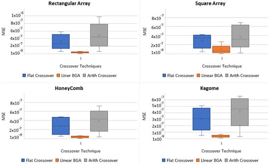
Figure 5. MSE comparison of various cross-over techniques on the selected geometries.

Table 2. Comparison of various ANN’s training algorithms as used in benchmark works.

Geometry	Training Algorithm					Epochs	MSE
	LM	CGF	CGB	CGP	BR
Square	✓					30	$5.73\times {10}^{-7}$
		✓				591	$9.41\times {10}^{-7}$
			✓			252	$2.33\times {10}^{-6}$
				✓		322	$6.21\times {10}^{-7}$
					✓	55	$2.08\times {10}^{-7}$
Rectangular	✓					39	$6.37\times {10}^{-7}$
		✓				478	$8.33\times {10}^{-6}$
			✓			767	$4.67\times {10}^{-6}$
				✓		388	$4.56\times {10}^{-7}$
					✓	69	$9.22\times {10}^{-8}$
HoneyComb	✓					54	$4.33\times {10}^{-7}$
		✓				634	$3.56\times {10}^{-7}$
			✓			276	$5.82\times {10}^{-7}$
				✓		376	$2.76\times {10}^{-7}$
					✓	67	$8.67\times {10}^{-8}$
Kagome	✓					43	$6.77\times {10}^{-7}$
		✓				476	$4.59\times {10}^{-7}$
			✓			291	$3.54\times {10}^{-7}$
				✓		463	$9.34\times {10}^{-7}$
					✓	79	$8.56\times {10}^{-8}$

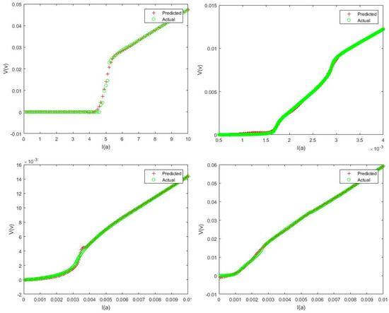
Figure 6. Predicted vs. measured IV characteristics.

6. Conclusions

Being predominantly dependent upon random initial conditions, the generated network’s coefficients mostly force the artificial neural networks to converge to a different local minima on every execution. This generally leads to an inconsistent prediction accuracy, even for identical experimental setup and tunable parameters. In this work, we have proposed an entropy based genetic algorithm, and used it to control the randomness in coefficient generation. This technique forces the network to converge (close) to the global minima on every execution, which constrains the prediction accuracy, measured in mean-squared error, to a certain acceptable level. We have applied our technique to approximate the current–voltage curves for four different lattices on a superconducting film, and compared our results with three recent works, which made use of artificial neural networks to achieve the same. Our results have shown that the proposed methodology yields better consistence and greater prediction accuracy.

References

- Acharya, S.; Bangera, K.V.; Shivakumar, G.K. Electrical characterization of vacuum-deposited p-CdTe/n-ZnSe heterojunctions. Appl. Nanosci. 2015, 5, 1003–1007. [Google Scholar] [CrossRef]
- Cleuziou, J.P.; Wernsdorfer, W.; Andergassen, S.; Florens, S.; Bouchiat, V.; Ondarçuhu, T.; Monthioux, M. Gate-tuned high frequency response of carbon nanotube Josephson junctions. Phys. Rev. Lett. 2007, 99, 117001. [Google Scholar] [CrossRef] [PubMed]
- Dinsmore, R.C., III; Bae, M.H.; Bezryadin, A. Fractional order Shapiro steps in superconducting nanowires. Appl. Phys. Lett. 2008, 93, 192505. [Google Scholar] [CrossRef]
- Mandal, S.; Naud, C.; Williams, O.A.; Bustarret, É.; Omnès, F.; Rodière, P.; Meunier, T.; Saminadayar, L.; Bäuerle, C. Detailed study of superconductivity in nanostructured nanocrystalline boron doped diamond thin films. Phys. Status Solidi 2010, 207, 2017–2022. [Google Scholar] [CrossRef]
- Kamran, M.; He, S.-K.; Zhang, W.-J.; Cao, W.-H.; Li, B.-H.; Kang, L.; Chen, J.; Wu, P.-H.; Qiu, X.-G. Matching effect in superconducting NbN thin film with a square lattice of holes. Chin. Phys. B 2009, 18, 4486. [Google Scholar] [CrossRef]
- Heiselberg, P. Shapiro steps in Josephson Junctions. Niels Bohr Institute, University of Copenhagen. 2013. Available online: https://cmt.nbi.ku.dk/student_projects/bsc/heiselberg.pdf (accessed on 13 July 2018).
- Sidorenko, A.; Zdravkov, V.; Ryazanov, V.; Horn, S.; Klimm, S.; Tidecks, R.; Wixforth, A.; Koch, T.; Schimmel, T. Thermally assisted flux flow in MgB2: Strong magnetic field dependence of the activation energy. Philos. Mag. 2005, 85, 1783–1790. [Google Scholar] [CrossRef]
- Fogel, N.Y.; Cherkasova, V.G.; Koretzkaya, O.A.; Sidorenko, A.S. Thermally assisted flux flow and melting transition for Mo/Si multilayers. Phys. Rev. B 1997, 55, 85. [Google Scholar] [CrossRef]
- Yu, C.C.; Chen, Y.T.; Wan, D.H.; Chen, H.L.; Ku, S.L.; Chou, Y.F. Using one-step, dual-side nanoimprint lithography to fabricate low-cost, highly flexible wave plates exhibiting broadband antireflection. J. Electrochem. Soc. 2011, 158, J195–J199. [Google Scholar] [CrossRef]
- Haider, S.A.; Naqvi, S.R.; Akram, T.; Kamran, M. Prediction of critical currents for a diluted square lattice using Artificial Neural Networks. Appl. Sci. 2017, 7, 238. [Google Scholar] [CrossRef]
- Haider, S.A.; Naqvi, S.R.; Akram, T.; Kamran, M.; Qadri, N.N. Modeling electrical properties for various geometries of antidots on a superconducting film. Appl. Nanosci. 2017, 7, 933–945. [Google Scholar] [CrossRef]
- Kamran, M.; Haider, S.A.; Akram, T.; Naqvi, S.R.; He, S.K. Prediction of IV curves for a superconducting thin film using artificial neural networks. Superlattices Microstruct. 2016, 95, 88–94. [Google Scholar] [CrossRef]
- Naqvi, S.R.; Akram, T.; Haider, S.A.; Kamran, M. Artificial neural networks based dynamic priority arbitration for asynchronous flow control. Neural Comput. Appl. 2016, 29, 627–637. [Google Scholar] [CrossRef]
- Güçlü, U.; van Gerven, M.A. Deep neural networks reveal a gradient in the complexity of neural representations across the ventral stream. J. Neurosci. 2015, 35, 10005–10014. [Google Scholar] [CrossRef] [PubMed]
- Haykin, S. Neural Networks and Learning Machines; Pearson: Upper Saddle River, NJ, USA, 2009; Volume 3. [Google Scholar]
- Zermeño, V.; Sirois, F.; Takayasu, M.; Vojenciak, M.; Kario, A.; Grilli, F. A self-consistent model for estimating the critical current of superconducting devices. Supercond. Sci. Technol. 2015, 28, 085004. [Google Scholar] [CrossRef]
- Bonanno, F.; Capizzi, G.; Graditi, G.; Napoli, C.; Tina, G.M. A radial basis function neural network based approach for the electrical characteristics estimation of a photovoltaic module. Appl. Energy 2012, 97, 956–961. [Google Scholar] [CrossRef]
- Naqvi, S.R.; Akram, T.; Iqbal, S.; Haider, S.A.; Kamran, M.; Muhammad, N. A dynamically reconfigurable logic cell: From artificial neural networks to quantum-dot cellular automata. Appl. Nanosci. 2018, 8, 89–103. [Google Scholar] [CrossRef]
- Haupt, R.L.; Haupt, S.E. Practical Genetic Algorithms; Wiley: New York, NY, USA, 1998; Volume 2. [Google Scholar]
- Herrera, F.; Lozano, M.; Sánchez, A.M. A taxonomy for the crossover operator for real-coded genetic algorithms: An experimental study. Int. J. Intell. Syst. 2003, 18, 309–338. [Google Scholar] [CrossRef]
- Razali, N.M.; Geraghty, J. Genetic algorithm performance with different selection strategies in solving TSP. In Proceedings of the World Congress on Engineering, London, UK, 6–8 July 2011; International Association of Engineers: Hong Kong, China, 2011; Volume 2, pp. 1134–1139. [Google Scholar]
- Mc Ginley, B.; Maher, J.; O’Riordan, C.; Morgan, F. Maintaining healthy population diversity using adaptive crossover, mutation, and selection. IEEE Trans. Evol. Comput. 2011, 15, 692–714. [Google Scholar] [CrossRef]
© 2018 by the authors. Licensee MDPI, Basel, Switzerland. This article is an open access article distributed under the terms and conditions of the Creative Commons Attribution (CC BY) license (http://creativecommons.org/licenses/by/4.0/).