RAISE: Robust and Adversarially Informed Safe Explanations for Reinforcement Learning

Abstract

Deep Reinforcement Learning (DRL) policies often exhibit fragility in unseen environments, limiting their deployment in safety-critical applications. While Robust Markov Decision Processes (R-MDPs) enhance control performance by optimizing against worst-case disturbances, the resulting conservative behaviors are difficult to interpret using standard Explainable RL (XRL) methods, which typically ignore adversarial disturbances. To bridge this gap, this paper proposes RAISE (Robust and Adversarially Informed Safe Explanations), a novel framework designed for the Noisy Action Robust MDP (NR-MDP) setting. We first introduce the Decomposed Reward NR-MDP (DRNR-MDP) and the DRNR-Deep Deterministic Policy Gradient (DRNR-DDPG) algorithm to learn robust policies and a vector-valued value function. RAISE utilizes this vectorized value function to generate contrastive explanations (“Why action $\mathbf{a}$ instead of $\mathbf{b}$?”), explicitly highlighting the reward components such as safety or energy efficiency prioritized under worst-case attacks. Experiments on a continuous Cliffworld benchmark and the MuJoCo Hopper task demonstrate that the proposed method preserves robust performance under dynamics variations and produces meaningful, component-level explanations that align with intuitive safety and performance trade-offs. Ablation results further show that ignoring worst-case disturbances can substantially alter or invalidate explanations, underscoring the importance of adversarial awareness for reliable interpretability in robust RL.

1. Introduction

Reinforcement learning (RL) has shown promising control performance when the training environment and the deployment environment are identical [1]. However, regarding the control law (policy) obtained by reinforcement learning, there exists a limitation that the robustness of the policy is insufficient when the deployment environment differs from the training environment, such as in autonomous driving [2,3], robot control [4,5,6], and smart factories [7,8,9]. Reinforcement learning assumes that the environment during training and the environment during deployment are identical, and if this assumption is not followed, the control performance of the policy cannot be guaranteed. In the field of autonomous driving, there are reports that control performance degrades as the road friction coefficient fluctuates due to rain or snow [10,11]. Thus, it is known that minor differences in environmental parameters between the training environment and the deployment environment cause a decline in control performance. In this paper, robustness refers to the property that can suppress the decline of control performance in the worst case, even if fluctuations in environmental parameters or disturbances not anticipated during training occur. In particular, the absence of policy robustness is a major obstacle preventing the introduction of reinforcement learning in fields where safety is important.

To address such robustness issues, a framework called Robust Markov Decision Process (R-MDP), which mathematically models the uncertainty of the deployment environment, has been studied. R-MDP considers two agents: a protagonist trying to maximize control performance and an adversary aiming to minimize control performance [12,13,14,15,16]. The protagonist learns a policy to achieve maximum control performance against the worst-case disturbance provided by the adversary. Consequently, it is guaranteed that the control performance of the protagonist’s policy will be above a certain level against any disturbance within the set of disturbances anticipated during training, and improvement in robust performance can also be expected.

In the R-MDP framework, the specific subclass is determined by the element of the MDP to which the adversarial disturbance is applied. For example, the adversarial disturbance may cause changes to the state transition function or the state [13], or it may act in the form of an external force [12]. However, such disturbances are physically difficult to implement in a real environment. To overcome this limitation, Noisy action Robust MDP (NR-MDP), which adds adversarial disturbances to the action, has been proposed [14], enabling the learning of robust policies even in real environments.

However, in order to apply policies to real environments, especially safety-critical environments, not only robustness but also policy explainability is required [17,18,19]. Even if mathematically optimal control performance is guaranteed, unless human users can understand the rationale for the agent’s action decisions and trust it, deployment in the real world is difficult. In particular, when the agent selects an unexpected action, an explanation of the action selection is necessary to distinguish whether that action conforms to the designer’s intent or is a result of incorrect learning.

On the other hand, since robust policies consider not only the maximization of control performance but also the influence of the adversary, there are limitations in explaining robust policies using conventional explanation methods. The behavior of the protagonist learned in the R-MDP setting is the result of defensive optimization preparing for the worst-case disturbance, in addition to maximizing control performance. Therefore, it may exhibit action selection with conservative patterns. In this case, it is difficult to accurately grasp the intent of the policy using only existing explainable RL (XRL) methods for the following reason: Conventional XRL methods assume that the policy aims to maximize control performance [17,18,19], whereas robust policies aim to maximize the lower bound of control performance against the worst-case disturbance. In other words, while many existing XRL methods assume the maximization of the policy’s control performance or the consistency of training and deployment environments, R-MDP does not follow these assumptions. Furthermore, to the best of the authors’ knowledge, no research satisfying both robust reinforcement learning and explainability simultaneously has been reported to date.

Therefore, in this study, we focus on presenting the rationale for action selection to achieve both robustness and explainability in the NR-MDP setting, so that users can use the system with confidence. To this end, to enable users to understand the decision-making process of the policy, we answer the question: “Why choose action $\mathbf{a}$ instead of action $\mathbf{b}$?” First, we introduce Decomposed Reward Noisy action Robust MDP (DRNR-MDP), which incorporates decomposed rewards into the NR-MDP setting, show that its theoretical optimal policy is equivalent to the theoretical optimal solution of the original NR-MDP, and propose the algorithm DRNR-Deep Deterministic Policy Gradient (DRNR-DDPG) to solve DRNR-MDP. Then, we propose RAISE (Robust and Adversarially Informed Safe Explanations), a framework that presents the rationale for the action selection of the obtained robust policy. In particular, RAISE presents the rationale regarding which reward component’s degradation the optimal action $\mathbf{a}$ prevented against the worst-case disturbance, compared to the comparison action $\mathbf{b}$ presented by the user. Thereby, we achieve the simultaneous provision of the robust policy and the rationale for its action selection.

To summarize, our contributions are as follows:

• We introduce a robust Bellman update rule for decomposed rewards within the NR-MDP framework and provide a theoretical guarantee of its convergence in tabular cases.
• We propose a method to quantitatively explain the agent’s choice of an action by comparing it against an alternative action ($\mathbf{a}$ vs. $\mathbf{b}$) based on decomposed reward components under shared adversarial disturbance.
• We conduct extensive experiments to demonstrate that our proposed framework, RAISE, not only learns robust policies but also provides reliable and insightful explanations.

2. Related Works

Domain Randomization: Domain Randomization (DR) exists as a method for learning robust policies. DR aims to learn a more generalized policy by having the agent experience diverse environmental parameters during training. For example, to bridge the reality gap between the simulator and the actual machine, there are methods that train the agent while randomly varying camera angles, lighting brightness, robot weight, etc. during training [20,21]. As a result, it succeeded in demonstrating excellent control performance on real machines without additional training. Also, in recent years, research has focused on environmental parameter sampling methods that maximize generalization performance, rather than changing environmental parameters randomly [22]. Consequently, diverse DR research has been advanced, and currently, it has achieved significant development such that even for complex tasks, policies can be applied in the real world after training in a simulator [20,21].

However, DR aims to increase the generalization performance of the policy and does not explicitly improve control performance against the worst-case disturbance. Therefore, there exists an aspect that makes it difficult to apply DR to safety-critical situations.

Robust RL: Robust RL (RRL) exists as a method to explicitly maximize control performance in worst-case disturbances. In robust reinforcement learning (RRL), a robust Markov decision process (R-MDP) is commonly used to model environmental uncertainties. Generally, the objective function of R-MDP is described as a max-min optimization problem where the protagonist maximizes control performance against the worst-case disturbance of the adversary [23].

Subclasses of R-MDP are determined by the type of the defined adversary actions. In early RRL research, directly changing the state transition function of the controlled object was common [24]. However, applying disturbances is difficult in situations where the state transition function cannot be directly manipulated or is even unknown. Besides frameworks that directly handle state transition functions, methods that apply disturbances in the form of external forces [12] or by changing the state of the controlled object [13] have been proposed. However, designing such disturbances is also difficult to implement physically in real environments. In recent years, Noisy action Robust MDP (NR-MDP) [14], a framework that adds disturbances to actions, has been proposed, making the realization of disturbances easier even in real environments.

As described above, diverse frameworks exist within R-MDP, and various algorithms exist to solve them [13,14,15,16]. Furthermore, these algorithms are generally based on iteratively solving minimization and maximization problems. While policies learned in this manner possess excellent robust performance, they often make it difficult for designers or users to intuitively understand the rationale for action selection due to their conservative actions against disturbances.

Explainable RL: As situations where safety is emphasized for reinforcement learning agents have arisen, understanding the agent’s behavior has become a requirement, and the field of Explainable Reinforcement Learning (XRL) has emerged in recent years. Bastani et al. [25] distilled a neural-network policy into a human-interpretable decision tree (policy extraction), thereby improving policy interpretability while accepting a certain degree of performance degradation. Similarly, Verma et al. [26] converted a neural-network policy into a high-level, domain-specific programming language, presenting the policy in a rule-based and interpretable form. However, these approaches share a common limitation: they follow a post hoc pipeline in which a neural policy is trained first and then an additional interpretable surrogate model is learned, which (i) incurs extra training/inference cost and (ii) may not faithfully preserve the original policy’s decision-making process, thereby limiting explanation fidelity.

A variety of XRL methods that do not rely on a post hoc pipeline have also been actively studied. For example, Madumal et al. [18] utilized a Structural Causal Model (SCM) and proposed a method to grasp, via a graph, how the action selected by the agent influences state transitions or reward components. Furthermore, Kim et al. [19] calculated the Shapley value for each state component in the value function to confirm which reward component the agent intends to maximize, and proposed a method to grasp the agent’s intent by identifying which reward component’s value the selected action maximizes. However, all of these methods share a key limitation: they require access to the structural causal model (SCM) of the controlled system. In contrast, Juozapaitis et al. propose an XRL approach that can be applied even when the SCM is unknown [17]. Their method represents the reward as a vector of a few semantically meaningful components and explains the agent’s intent by identifying which reward components are most responsible for the selected action. Of course, this approach is not applicable in settings where the reward function is unknown or cannot be decomposed. However, in many real-world tasks, such as autonomous driving [27] and financial portfolio management [28], it is common to define multiple reward components separately at the design stage. In such problem settings, the research of Juozapaitis et al. [17] can provide useful reasons for decision-making choices.

These XRL methods possess a fundamental limitation when it comes to correctly explaining robust policies. In this context, providing explanations for a robust policy means explaining why an action is selected while accounting for worst-case disturbances. Existing XRL methods provide explanations based on the assumption that the agent aims to maximize control performance. On the other hand, the objective function of general R-MDP frameworks, including NR-MDP, is a max-min optimization problem that considers the effects of disturbances, and thus does not follow the assumption of XRL. For this reason, there is a limitation that the agent’s rational defensive behaviors against potential threats cannot be correctly explained. Building on reward decomposition setting, our work directly addresses this gap by creating an explanation framework that is inherently aware of the adversarial nature of the NR-MDP setting. In addition, to clarify the positioning of our work, Table 1 summarizes the key characteristics of prior XRL studies and our approach.

Table 1. Comparison of representative XRL methods and our approach, highlighting (i) support for continuous actions, (ii) whether explanations are intrinsic or post hoc, (iii) the key assumptions (e.g., SCM access or decomposed rewards), and (iv) whether the method can explain robust action selection under worst-case disturbances.

Method	Continuous	Intrinsic?	Key Assumption	Robust-Policy
Bastani [25]	Not reported	No (post hoc)	None	No
Verma [26]	Yes	No (post hoc)	None	No
Madumal [18]	No	Yes	SCM access	No
Kim [19]	Yes	Yes	SCM access	No
Juozapaitis [17]	Yes	Yes	Decomposed reward	No
Ours	Yes	Yes	Decomposed reward	Yes

3. Preliminaries

3.1. Markov Decision Process

An MDP is defined as a tuple $(\mathcal{S},\mathcal{A},R,P,\gamma )$ [29]. Here, $\mathcal{S}$ is the set of states, $\mathcal{A}$ is the set of actions, $R:\mathcal{S}\times \mathcal{A}\to \mathbb{R}$ is the reward function, $P:\mathcal{S}\times \mathcal{A}\times \mathcal{S}\to [0,1]$ is the state transition function, and $\gamma \in [0,1)$ is the discount factor. In this study, we specifically consider continuous action spaces.

Next, we describe the objective function of reinforcement learning. In reinforcement learning, the goal is to maximize the control performance of a policy $\pi$. In this study, we consider a deterministic policy $\pi :\mathcal{S}\to \mathcal{A}$ where an action is uniquely determined given a state input. The objective of reinforcement learning is to find a policy that maximizes control performance, which can be expressed as finding the policy ${\pi }^{\ast }={arg\; max}_{\pi }{V}^{\pi }\left(\mathbf{s}\right)$ that maximizes the value function

$$V^{\pi }\left(\mathbf{s}\right)={\mathbb{E}}_{\pi }\left[\sum _{t=0}^{\infty }{\gamma }^{t}r({\mathbf{s}}_t,{\mathbf{a}}_t)|{\mathbf{s}}_0=\mathbf{s}\right]$$

for an arbitrary state $\mathbf{s}$. Alternatively, it can be expressed as ${\pi }^{\ast }={arg\; max}_{\pi }{Q}^{\pi }(\mathbf{s},\pi \left(\mathbf{s}\right))$ using the action-value function:

$$Q^{\pi }(\mathbf{s},\mathbf{a})={\mathbb{E}}_{\pi }\left[\sum _{t=0}^{\infty }{\gamma }^{t}r({\mathbf{s}}_t,{\mathbf{a}}_t)|{\mathbf{s}}_0=\mathbf{s},{\mathbf{a}}_0=\mathbf{a}\right].$$

Here, the Bellman optimality operator is defined as

$$\left(T^{\ast }Q\right)(\mathbf{s},\mathbf{a})=r(\mathbf{s},\mathbf{a})+\gamma {\mathbb{E}}_{{\mathbf{s}}^{\prime }\sim P(·|\mathbf{s},\mathbf{a})}[\underset{{\mathbf{a}}^{\prime }\in \mathcal{A}}{max}Q({\mathbf{s}}^{\prime },{\mathbf{a}}^{\prime })].$$

If the reward function is bounded, iteratively applying this operator converges to the unique optimal action-value function $Q^{\ast }$ that satisfies

$$Q^{\ast }(\mathbf{s},\mathbf{a})=r(\mathbf{s},\mathbf{a})+\gamma {\mathbb{E}}_{{\mathbf{s}}^{\prime }\sim P(·|\mathbf{s},\mathbf{a})}[\underset{{\mathbf{a}}^{\prime }\in \mathcal{A}}{max}{Q}^{\ast }({\mathbf{s}}^{\prime },{\mathbf{a}}^{\prime })].$$

The optimal policy satisfies

$${\pi }^{\ast }\left(\mathbf{s}\right)\in arg\underset{\mathbf{a}\in \mathcal{A}}{max}{Q}^{\ast }(\mathbf{s},\mathbf{a})(\forall \mathbf{s}\in \mathcal{S}).$$

3.2. Noisy-Action Robust MDP

NR-MDP is defined as $(\mathcal{S},\mathcal{A},R,P,\gamma ,\alpha )$ similar to MDP, where $\alpha \in [0,1]$ represents the strength of the adversarial disturbance mixed into the executed action [14]. In this study, we assume that the protagonist policy ${\pi }^P$ and the adversary policy ${\pi }^A$ are deterministic. In the NR-MDP setting, the action

$$m_{\alpha }({\mathbf{a}}^P,{\mathbf{a}}^A):=(1-\alpha ){\mathbf{a}}^P+\alpha {\mathbf{a}}^A$$

which is mixed from the protagonist action ${\mathbf{a}}^P$ and the adversary action ${\mathbf{a}}^A$, is executed.

Next, we describe the objective function of the NR-MDP. Let us denote ${\pi }^m\left(\mathbf{s}\right)=m_{\alpha }({\pi }^P\left(\mathbf{s}\right),{\pi }^A\left(\mathbf{s}\right))$. In this case, the objective function of the NR-MDP becomes ${max}_{{\pi }^P}{min}_{{\pi }^A}$$V^{{\pi }^m}\left(\mathbf{s}\right)$. Furthermore, utilizing the Q-function, it can also be described as ${max}_{{\pi }^P}{min}_{{\pi }^A}$$Q^{{\pi }^m}(\mathbf{s},{\pi }^m\left(\mathbf{s}\right))$.

Finally, we describe the relationship between the Bellman robust operator and the optimal policy in the NR-MDP. We define the Bellman robust operator in the NR-MDP as

$$\begin{array}{cc}\hfill & \left({\mathcal{B}}_{\mathrm{NR}}^{\ast }Q\right)(\mathbf{s},m_{\alpha }({\mathbf{a}}^P,{\mathbf{a}}^A))\hfill \\ \hfill =& r(\mathbf{s},m_{\alpha }({\mathbf{a}}^P,{\mathbf{a}}^A))+\gamma {\mathbb{E}}_{{\mathbf{s}}^{\prime }}[\underset{{\mathbf{a}}^{P^{\prime }}}{max}\underset{{\mathbf{a}}^{A^{\prime }}}{min}Q({\mathbf{s}}^{\prime },m_{\alpha }({\mathbf{a}}^{P^{\prime }},{\mathbf{a}}^{A^{\prime }}))].\hfill \end{array}$$

Then, the optimal action-value function $Q^{\ast }$ satisfies

$$\begin{array}{cc}\hfill & Q^{\ast }(\mathbf{s},m_{\alpha }({\mathbf{a}}^P,{\mathbf{a}}^A))\hfill \\ \hfill =& r(\mathbf{s},m_{\alpha }({\mathbf{a}}^P,{\mathbf{a}}^A))+\gamma {\mathbb{E}}_{{\mathbf{s}}^{\prime }}[\underset{{\mathbf{a}}^{P^{\prime }}}{max}\underset{{\mathbf{a}}^{A^{\prime }}}{min}{Q}_m^{\ast }({\mathbf{s}}^{\prime },m_{\alpha }({\mathbf{a}}^{P^{\prime }},{\mathbf{a}}^{A^{\prime }}))]\hfill \end{array}$$

and the optimal protagonist policy satisfies

$${\pi }^{P\ast }\left(\mathbf{s}\right)=\underset{{\mathbf{a}}^P}{arg\; max}\underset{{\mathbf{a}}^A}{min}{Q}^{\ast }(\mathbf{s},m_{\alpha }({\mathbf{a}}^P,{\mathbf{a}}^A))$$

Similar to general MDPs, it is known that iterating ${\mathcal{B}}_{\mathrm{NR}}^{\ast }$ converges to the unique optimal action-value function.

3.3. Reward Decomposition

Reward decomposition defines the original scalar reward r as a vector with several meaningful components to interpret the agent’s decision-making process [17]. For example, in the case of a racecar, it is expressed as the sum of several sub-goals, such as goal reaching, energy efficiency, and safety maintenance. While reward decomposition may be infeasible in some settings (e.g., black-box reward models or sparse-reward problems), this work focuses on tasks where the reward is specified as a sum of semantically meaningful components by the system designer. Our study likewise adopts this assumption.

More generally, letting $\mathcal{C}$ be the set of reward components, the decomposed reward is denoted as $\overrightarrow{r}$, and the reward of the component $c\in \mathcal{C}$ is denoted as ${\overrightarrow{r}}_c$. Furthermore, the action-value function $\overrightarrow{Q}$ is defined as

$${\overrightarrow{Q}}^{\pi }(\mathbf{s},\mathbf{a})={\mathbb{E}}_{\pi }\left[\sum _{t=0}^{\infty }{\gamma }^t\overrightarrow{r}({\mathbf{s}}_t,{\mathbf{a}}_t)|{\mathbf{s}}_0=\mathbf{s},{\mathbf{a}}_0=\mathbf{a}\right].$$

Here, the sum of the components of $\overrightarrow{Q}$ is identical to the action value in general reinforcement learning, and the optimal policy is defined as

$$\begin{array}{cc}\hfill {\pi }^{\ast }=& \underset{\pi }{arg\; max}\sum _{c\in \mathcal{C}}{\overrightarrow{Q}}_c^{\pi }(\mathbf{s},\pi \left(\mathbf{s}\right)).\hfill \end{array}$$

(1)

To solve this objective, Juozapaitis et al. [17] proposed Decomposed reward Q-Learning (DrQ). This algorithm learns component-wise action-value functions in a Q-learning style and defines the policy by selecting the action that maximizes the sum of the component-wise action-value functions. However, since Q-learning is not directly applicable to continuous action spaces, we compare our method with Decomposed reward DDPG (DR-DDPG), which follows the same decomposition idea but uses a DDPG-style optimization procedure instead of Q-learning, as well as with our proposed method.

Once the ${\overrightarrow{Q}}^{{\pi }^{\ast }}$ function and the optimal policy ${\pi }^{\ast }$ have been learned, the interpretation of actions is required. In this context, to quantitatively verify the reason why ${\pi }^{\ast }\left(\mathbf{s}\right)$ is optimal compared to a certain action $\mathbf{b}$, the difference for each Q-component defined as $\overrightarrow{\Delta }(\mathbf{s},{\pi }^{\ast }\left(\mathbf{s}\right),\mathbf{b})={\overrightarrow{Q}}^{{\pi }^{\ast }}(\mathbf{s},{\pi }^{\ast }\left(\mathbf{s}\right))-{\overrightarrow{Q}}^{{\pi }^{\ast }}(\mathbf{s},\mathbf{b})$ is used. This allows us to identify in terms of which reward components the selection of ${\pi }^{\ast }\left(\mathbf{s}\right)$ is superior to $\mathbf{b}$.

Furthermore, Minimal Sufficient Explanations (MSX) have been proposed Juozapaitis et al. to present the critical minimal rationale for action selection [17]. They divide the set of reward components $\mathcal{C}$ into components that are disadvantageous and advantageous for $\mathbf{a}$:

$$\begin{array}{cc}\hfill {\mathcal{C}}^{-}& :=\{c\in \mathcal{C}\mid {\overrightarrow{\Delta }}_c<0\},\hfill \\ \hfill {\mathcal{C}}^{+}& :=\{c\in \mathcal{C}\mid {\overrightarrow{\Delta }}_c>0\}.\hfill \end{array}$$

The components belonging to ${\mathcal{C}}^{-}$ represent the “reward aspects where $\mathbf{a}$ performs worse than $\mathbf{b}$,” while ${\mathcal{C}}^{+}$ represents the reward aspects where $\mathbf{a}$ improves upon $\mathbf{b}$. Let the “total loss” caused by the negative components as

$$K:=\sum _{c\in {\mathcal{C}}^{-}}\left|{\overrightarrow{\Delta }}_c\right|=-\sum _{c\in {\mathcal{C}}^{-}}{\overrightarrow{\Delta }}_c(\ge 0).$$

Then, the minimal set of positive components ${\mathcal{C}}_{exp}^{+}\subseteq {\mathcal{C}}^{+}$ sufficient to offset this loss K is as follows:

$${\mathcal{C}}_{exp}^{+}:=arg\underset{\mathcal{S}\subseteq {\mathcal{C}}^{+}}{min}\left\{|\mathcal{S}||\sum _{c\in \mathcal{S}}{\overrightarrow{\Delta }}_c\ge K\right\}.$$

That is, ${\mathcal{C}}_{exp}^{+}$ is determined as the subset with the smallest cardinality satisfying ${\sum }_{c\in {\mathcal{C}}_{exp}^{+}}{\overrightarrow{\Delta }}_c\ge K$. Intuitively, ${\mathcal{C}}_{exp}^{+}$ represents the minimal set of reward components that are prioritized for improvement by selecting $\mathbf{a}$, even at the cost of tolerating “some deterioration (${\mathcal{C}}^{-}$).”

4. Proposed Method

In this study, we aim to develop a method that provides the explanation for the policy’s action decisions while maintaining robust performance. Therefore, we aim to answer the following question: “Why choose action $\mathbf{a}$ instead of action $\mathbf{b}$?” To answer this question, following the work of Juozapaitis et al. [17], we learn robust action values for each reward component in problem settings where the reward function is decomposed into multiple human-interpretable semantic elements (e.g., safety, efficiency, comfort). In conventional NR-MDPs, since the agent seeks to maximize a final single Q-value (scalar value), it is impossible to distinguish why that Q-value is robust (e.g., whether efficiency was preserved at the expense of safety, or vice versa). In this study, we consider learning Q-values as a vector $\overrightarrow{Q}=[Q_{\mathrm{safety}},Q_{\mathrm{speed}},\dots ]$ rather than a scalar. Thereby, while maintaining the robust performance of the policy, we simultaneously achieve the provision of analysis regarding “what kind of worst-case disturbance the agent anticipates” and “which reward components were considered against that disturbance.”

To achieve this objective, we propose two primary frameworks in this section. First, we define a new framework called DRNR-MDP (Decomposed Reward Noisy action Robust MDP), which is an NR-MDP setting with decomposed rewards, and propose a practical DDPG-based algorithm, DRNR-DDPG, to solve it. This algorithm simultaneously acquires a robust policy and learns a decomposed Q-value vector $\overrightarrow{Q}$ that serves as the basis for explanation. Second, using the learned policy and $\overrightarrow{Q}$ function, we propose an explanation framework RAISE (Robust and Adversarially Informed Safe Explanations) to answer the aforementioned question by extending the MSX explanation method.

4.1. Decomposed Reward NR-MDP

In this section, we define the Decomposed Reward NR-MDP (DRNR-MDP), the theoretical framework within which DRNR-DDPG is learned. We then introduce the objective function and the Bellman robust operator of the DRNR-MDP.

The DRNR-MDP is defined by the tuple ${\mathcal{M}}_{DR}=(\mathcal{S},\mathcal{A},P,\overrightarrow{R},\gamma ,\alpha )$, sharing many components with the standard NR-MDP. The only difference is that the reward function $\overrightarrow{R}:\mathcal{S}\times \mathcal{A}\to {\mathbb{R}}^{\left|\mathcal{C}\right|}$ returns a $\left|\mathcal{C}\right|$-dimensional vector. Here, $\mathcal{C}$ is the set of reward components. Then, the objective function of the DRNR-MDP is formulated as ${max}_{{\pi }^P}{min}_{{\pi }^A}{V}^{{\pi }^m}\left(\mathbf{s}\right)$ with respect to

$$\begin{array}{cc}\hfill & V^{{\pi }^m}\left(\mathbf{s}\right)={\mathbb{E}}_{{\pi }^m}\left[\sum _{t=0}^{\infty }{\gamma }^t\sum _{c\in \mathcal{C}}{\overrightarrow{r}}_c({\mathbf{s}}_t,m_{\alpha }({\mathbf{a}}_t^P,{\mathbf{a}}_t^A))|{\mathbf{s}}_0=\mathbf{s}\right].\hfill \end{array}$$

Next, we define the Bellman robust operator ${\mathcal{B}}_{\mathcal{DR}}^{\ast }$ in the DRNR-MDP:

$$\begin{array}{cc}\hfill & \left({\mathcal{B}}_{\mathcal{DR}}^{\ast }\overrightarrow{Q}\right)(\mathbf{s},m_{\alpha }({\mathbf{a}}^P,{\mathbf{a}}^A))\hfill \\ \hfill =& \overrightarrow{r}(\mathbf{s},m_{\alpha }({\mathbf{a}}^P,{\mathbf{a}}^A))+\gamma {\mathbb{E}}_{{\mathbf{s}}^{\prime }}\left[\overrightarrow{Q}({\mathbf{s}}^{\prime },m_{\alpha }({\mathbf{a}}^{P\ast },{\mathbf{a}}^{A\ast }))\right],\hfill \\ \hfill & \mathrm{where}({\mathbf{a}}^{P\ast },{\mathbf{a}}^{A\ast })=\arg \underset{{\mathbf{a}}^{P^{\prime }}}{max}\underset{{\mathbf{a}}^{A^{\prime }}}{min}\sum _{c\in \mathcal{C}}{\overrightarrow{Q}}_c({\mathbf{s}}^{\prime },m_{\alpha }({\mathbf{a}}^{P^{\prime }},{\mathbf{a}}^{A^{\prime }})).\hfill \end{array}$$

While the Bellman robust operator in the NR-MDP is applied to a scalar-valued Q-function, the Bellman robust operator in the DRNR-MDP is applied to a vector-valued Q-function. An important point to note is that our objective function does not optimize each component-wise action-value function ${\overrightarrow{Q}}_c^{\pi }$ separately; rather, it optimizes a single scalar objective defined by their sum, ${\sum }_{c\in \mathcal{C}}{\overrightarrow{Q}}_c^{\pi }$. That is, our setting is not multi-objective RL, where different policies are learned for multiple objectives, but a single-objective robust RL setting in which the objective is defined as the sum over components, and the component-wise ${\overrightarrow{Q}}_c^{\pi }$ are merely a decomposed representation for providing explanations.

Here, both the protagonist and the adversary aim to maximize and minimize the sum of the components of $\overrightarrow{Q}$, respectively. In the subsequent section, we show that iterating the defined Bellman robust operator ${\mathcal{B}}_{DR}^{\ast }$ sufficiently causes the sum of the components ${\sum }_{c\in \mathcal{C}}{\overrightarrow{Q}}_c(\mathbf{s},\mathbf{a})$ to converge to the optimal action-value function $Q^{\ast }(\mathbf{s},\mathbf{a})$ of the standard NR-MDP, and consequently, the resulting optimal policy is equivalent to that of the conventional NR-MDP.

4.2. Theoretical Properties of DRNR-MDP

In this section, we establish the theoretical validity of the DRNR-MDP. The objective of this study is to achieve explainability through reward decomposition while preserving the robust optimality guaranteed by the original NR-MDP. To ensure this, we prove that the proposed Bellman robust operator ${\mathcal{B}}_{\mathcal{DR}}^{\ast }$ of the DRNR-MDP satisfies the following property: the sum of components ${\sum }_{c\in \mathcal{C}}{\overrightarrow{Q}}_c^{\ast }$ of the converged fixed point ${\overrightarrow{Q}}^{\ast }$ coincides with the optimal action-value function $Q_{NR}^{\ast }$ of the original NR-MDP. To this end, starting with the relationship between ${\mathcal{B}}_{\mathrm{DR}}^{\ast }$ and ${\mathcal{B}}_{\mathrm{NR}}^{\ast }$, we show that this property holds through Proposition 1, Lemma 1, Theorem 1, and Corollaries.

First, the following relationship holds between ${\mathcal{B}}_{\mathrm{DR}}^{\ast }$ and ${\mathcal{B}}_{\mathrm{NR}}^{\ast }$.

Proposition 1

(Closure property of summation). The following equality holds for any $\overrightarrow{Q}$:

$$\sum _c{\left({\mathcal{B}}_{DR}^{\ast }\overrightarrow{Q}\right)}_c={\mathcal{B}}_{NR}^{\ast }\left(\sum _c{\overrightarrow{Q}}_c\right).$$

Proof 

sketch. $({\mathbf{a}}^{P\ast },{\mathbf{a}}^{A\ast })$ is defined based on ${\sum }_{c\in \mathcal{C}}{\overrightarrow{Q}}_c$. Due to the linearity of summation, the sum of the components on the left-hand side coincides with the operation of ${\mathcal{B}}_{NR}^{\ast }$ on the right-hand side.    □

From this proposition, it is understood that when each Q-function component is updated according to ${\mathcal{B}}_{\mathrm{DR}}^{\ast }$, the sum of the components behaves identically to the update of ${\mathcal{B}}_{\mathrm{NR}}^{\ast }$.

Next, we demonstrate the ∞-Lipschitz property of the max-min operator.

Lemma 1

(∞-Lipschitz property of $maxmin$). For bounded functions $U,V:\mathcal{A}\times \mathcal{A}\to \mathbb{R}$, the following inequality holds:

$$\begin{array}{cc}\hfill & |\underset{{\mathbf{a}}^P}{max}\underset{{\mathbf{a}}^A}{min}U({\mathbf{a}}^P,{\mathbf{a}}^A)-\underset{{\mathbf{a}}^P}{max}\underset{{\mathbf{a}}^A}{min}V({\mathbf{a}}^P,{\mathbf{a}}^A)|\hfill \\ \hfill \le & \underset{{\mathbf{a}}^P,{\mathbf{a}}^A}{max}|U-V|.\hfill \end{array}$$

Proof. 

Let $\delta :={\parallel U-V\parallel }_{\infty }$. Then, for any $({\mathbf{a}}^P,{\mathbf{a}}^A)$, we have $V-\delta \le U\le V+\delta$. Therefore, for each ${\mathbf{a}}^P$,

$$\underset{{\mathbf{a}}^A}{min}V-\delta \le \underset{{\mathbf{a}}^A}{min}U\le \underset{{\mathbf{a}}^A}{min}V+\delta .$$

Furthermore, since applying ${max}_{{\mathbf{a}}^P}$ preserves these bounds, we obtain

$$|\underset{{\mathbf{a}}^P}{max}\underset{{\mathbf{a}}^A}{min}U-\underset{{\mathbf{a}}^P}{max}\underset{{\mathbf{a}}^A}{min}V|\le \delta ={\parallel U-V\parallel }_{\infty }.$$

   □

By employing Lemma 1, it can be shown that ${\mathcal{B}}_{NR}^{\ast }$ is a $\gamma$-contraction, ensuring the convergence of ${\mathcal{B}}_{NR}^{\ast }$.

Theorem 1

($\gamma$-contraction of ${\mathcal{B}}_{NR}^{\ast }$). For any bounded functions $Q_1,Q_2:\mathcal{S}\times \mathcal{A}\to \mathbb{R}$,

$$\parallel {\mathcal{B}}_{NR}^{\ast }{Q}_1-{\mathcal{B}}_{NR}^{\ast }{Q}_2{\parallel }_{\infty }\le \gamma {\parallel Q_1-Q_2\parallel }_{\infty }.$$

Proof. 

For any $(\mathbf{s},\mathbf{a})$,

$$\begin{array}{cc}& ({\mathcal{B}}_{NR}^{\ast }{Q}_1-{\mathcal{B}}_{NR}^{\ast }{Q}_2)(\mathbf{s},\mathbf{a})\hfill \\ & =\gamma {\mathbb{E}}_{{\mathbf{s}}^{\prime }}\left[\underset{{\mathbf{a}}^P}{max}\underset{{\mathbf{a}}^A}{min}{Q}_1({\mathbf{s}}^{\prime },m_{\alpha }({\mathbf{a}}^P,{\mathbf{a}}^A))-\underset{{\mathbf{a}}^P}{max}\underset{{\mathbf{a}}^A}{min}{Q}_2({\mathbf{s}}^{\prime },m_{\alpha }({\mathbf{a}}^P,{\mathbf{a}}^A))\right]\hfill \\ & \le \gamma {\mathbb{E}}_{{\mathbf{s}}^{\prime }}\left[\underset{{\mathbf{a}}^P,{\mathbf{a}}^A}{max}|Q_1({\mathbf{s}}^{\prime },m_{\alpha }({\mathbf{a}}^P,{\mathbf{a}}^A))-Q_2({\mathbf{s}}^{\prime },m_{\alpha }({\mathbf{a}}^P,{\mathbf{a}}^A))|\right]\hfill \\ \hfill & \le \gamma \parallel Q_1-Q_2{\parallel }_{\infty }.\hfill \end{array}$$

   □

The full proof of Theorem 1 is provided in Appendix A.

By utilizing the above proposition, lemma, and theorem, it is derived that the sum of the components of the action-value function obtained by sufficiently iterating ${\mathcal{B}}_{DR}^{\ast }$ is the optimal Q-function in the NR-MDP.

Corollary 1

(Existence and Uniqueness of Fixed Point and Iterative Convergence). Since ${\mathcal{B}}_{NR}^{\ast }$ is a γ-contraction, there exists a unique fixed point $Q_{NR}^{\ast }$. For any initial function $Q^{\left(0\right)}$,

$$Q^{(k+1)}={\mathcal{B}}_{NR}^{\ast }{Q}^{\left(k\right)}\Rightarrow Q^{\left(k\right)}\underset{k\to \infty }{\to }{Q}_{NR}^{\ast }.$$

Corollary 2

(Convergence of Component Sum to NR Optimal Q). From Proposition 1 and Corollary 1, for any ${\overrightarrow{Q}}^{\left(0\right)}$,

$$\begin{array}{cc}\hfill & {\Sigma }_c\left({\overrightarrow{Q}}_c^{(k+1)}\right)={\Sigma }_c\left({\mathcal{B}}_{DR}^{\ast }{\overrightarrow{Q}}_c^{\left(k\right)}\right)={\mathcal{B}}_{NR}^{\ast }\left({\Sigma }_c{\overrightarrow{Q}}_c^{\left(k\right)}\right)\hfill \\ \hfill & \Rightarrow {\Sigma }_c{\overrightarrow{Q}}_c^{\left(k\right)}\underset{k\to \infty }{\to }{Q}_{NR}^{\ast }.\hfill \end{array}$$

That is, the sum of the components ${\overrightarrow{Q}}_c$ converges to the optimal Q of the NR-MDP.

From Corollary 2, it is evident that the optimal protagonist in the DRNR-MDP is equivalent to the optimal policy in the NR-MDP in terms of robust performance, establishing it as a framework capable of incorporating explainability.

4.3. Decomposed Reward Noisy Action Robust DDPG (DRNR-DDPG)

In this section, we describe a method to heuristically obtain the theoretical optimal policy discussed in Section 4.1. We propose an algorithm based on the AR-DDPG proposed by Tessler et al. [14].

First, let ${\pi }^P\left(\mathbf{s}\right|{\theta }^P)$ denote the protagonist policy, ${\pi }^A\left(\mathbf{s}\right|{\theta }^A)$ denote the adversary policy, and ${\overrightarrow{Q}}_c(\mathbf{s},\mathbf{a}|{\varphi }_c)$ denote the action-value function for component $c\in \mathcal{C}$. Here, ${\theta }^P$, ${\theta }^A$, and ${\varphi }_c$ represent the parameters of the respective models, while ${\theta }^{P-}$, ${\theta }^{A-}$, and ${\varphi }_c^{-}$ represent the parameters of the target models.

Next, we examine the update rules for each parameter. The protagonist policy is updated to maximize the sum of the component-wise action values ${\sum }_{c\in \mathcal{C}}{\overrightarrow{Q}}_c$, while the adversary is updated to minimize ${\sum }_{c\in \mathcal{C}}{\overrightarrow{Q}}_c$. Consequently, ${\theta }^P$ and ${\theta }^A$ are updated as follows:

$$\begin{array}{cc}\hfill & \mathrm{Protagonist}:\hfill \\ \hfill & {\theta }^P\leftarrow {\theta }^P+{\mathbf{a}}^P{\nabla }_{{\theta }^P}J\hfill \\ \hfill & {\nabla }_{{\theta }^P}J={\mathbb{E}}_{\mathbf{s}}\left[\sum _{c\in \mathcal{C}}{\nabla }_{{\theta }^P}{\overrightarrow{Q}}_c\left(\mathbf{s},m_{\alpha }({\pi }^P\left(\mathbf{s}\right|{\theta }^P),{\pi }^A\left(\mathbf{s}\right|{\theta }^A))\right)\right],\hfill \\ \hfill & \mathrm{Antagonist}:\hfill \\ \hfill & {\theta }^A\leftarrow {\theta }^A-{\mathbf{a}}^A{\nabla }_{{\theta }^A}J\hfill \\ \hfill & {\nabla }_{{\theta }^A}J={\mathbb{E}}_{\mathbf{s}}\left[\sum _{c\in \mathcal{C}}{\nabla }_{{\theta }^A}{\overrightarrow{Q}}_c\left(\mathbf{s},m_{\alpha }({\pi }^P\left(\mathbf{s}\right|{\theta }^P),{\pi }^A\left(\mathbf{s}\right|{\theta }^A))\right)\right].\hfill \end{array}$$

The critic is trained to minimize the TD-error for all components $c\in \mathcal{C}$, and its loss function is defined as

$$\begin{array}{cc}\hfill & L_c=\left|\right|{\overrightarrow{r}}_c+\gamma {\overrightarrow{Q}}_c({\mathbf{s}}^{\prime },m_{\alpha }({\pi }^P\left(\mathbf{s}\right|{\theta }^{P-}),{\pi }^A\left(\mathbf{s}\right|{\theta }^{A-}))|{\varphi }_c^{-})\hfill \\ & -{\overrightarrow{Q}}_c(\mathbf{s},\mathbf{a}|{\varphi }_c){\left|\right|}_2^2.\hfill \end{array}$$

This loss function serves as an approximate implementation of the Bellman robust operator in the DRNR-MDP ${\mathcal{B}}_{DR}^{\ast }$, and similar formulations are employed in numerous reinforcement learning algorithms, including DDPG [30]. Although we presented an update method based on DDPG in this study, any algorithm utilizing Q-functions, such as TD3 [31], is applicable. The pseudocode for the model updates in the DDPG style is presented in Algorithm 1.

Algorithm 1 DRNR-DDPG

1: Input: Actor update steps (N), adversary update steps (M) uncertainty value ($\alpha$) and discount factor ($\gamma$) 2: Initialize critic network $Q(\mathbf{s},\mathbf{a}|\varphi )$, actor $f\left(\mathbf{s}\right|{\theta }^P)$ and adversary $g\left(\mathbf{s}\right|{\theta }^A)$ 3: Initialize target networks with weight ${\varphi }^{-},{\theta }^{P-},{\theta }^{A-}$ 4: Initialize replay buffer $\mathcal{R}$. 5: for episode in 0…M do 6:     Receive initial observation state ${\mathbf{s}}_0$ 7:     for $t=0$…T do 8:         Get action ${\mathbf{a}}_t=(1-\alpha )f({\mathbf{s}}_t;{\theta }^P)+\alpha g({\mathbf{s}}_t;{\theta }^A)$ 9:         Execute ${\tilde{\mathbf{a}}}_t={\mathbf{a}}_t+$ noise, observe reward $r_t$ and observe new state ${\mathbf{s}}_{t+1}$ 10:       Store transition $({\mathbf{s}}_t,{\tilde{\mathbf{a}}}_t,{\overrightarrow{r}}_t,{\mathbf{s}}_{t+1})$ in $\mathcal{R}$ 11:       for $i=0$…N do 12:           Sample batch from replay buffer 13:           for $c\in \mathcal{C}$ do 14:               Update critic: ${\varphi }_c\leftarrow -{\nabla }_{{\varphi }_c}\left|\right|{\overrightarrow{r}}_c+\gamma \left[{\overrightarrow{Q}}_c({\mathbf{s}}^{\prime },(1-\alpha )f({\mathbf{s}}^{\prime };{\theta }^{P-})+\alpha g({\mathbf{s}}^{\prime };{\theta }^{A-});{\varphi }_c^{-})\right]{\left|\right|}_2^2$ 15:           end for 16:           Update actor: ${\theta }^P\leftarrow -{\nabla }_{{\theta }^P}{\sum }_{c\in \mathcal{C}}{\overrightarrow{Q}}_c(\mathbf{s},(1-\alpha )f(\mathbf{s};{\theta }^P)+\alpha g(\mathbf{s};{\theta }^A);{\varphi }_c)$ 17:       end for 18:       for $i=0$…M do 19:           Sample batch from replay buffer 20:           for $c\in \mathcal{C}$ do 21:               Update critic: ${\varphi }_c\leftarrow -{\nabla }_{{\varphi }_c}\left|\right|{\overrightarrow{r}}_c+\gamma \left[{\overrightarrow{Q}}_c({\mathbf{s}}^{\prime },(1-\alpha )f({\mathbf{s}}^{\prime };{\theta }^{P-})+\alpha g({\mathbf{s}}^{\prime };{\theta }^{A-});{\varphi }_c^{-})\right]{\left|\right|}_2^2$ 22:           end for 23:           Update adversary: ${\theta }^A\leftarrow {\nabla }_{{\theta }^A}{\sum }_{c\in \mathcal{C}}{\overrightarrow{Q}}_c(\mathbf{s},(1-\alpha )f(\mathbf{s};{\theta }^P)+\alpha g(\mathbf{s};{\theta }^A);{\varphi }_c)$ 24:       end for 25:       Update the target networks 26:    end for 27: end for

Finally, we compare the proposed method’s training-time computational complexity, storage (space) complexity, and explanation-generation (inference) complexity against AR-DDPG and DR-DDPG (DDPG-style implementation of the reward-decomposition idea in Juozapaitis et al. [17] for continuous control). For the proposed method, per environment step (or per iteration), the protagonist policy is updated N times and the adversary policy is updated M times; for each policy update, the critic is updated once for each reward component $c\in \mathcal{C}$, resulting in $\left|\mathcal{C}\right|$ critic updates.

Let $T_s$ denote the computational cost of one environment interaction, $T_{\mathrm{Prota}}$ the cost of one protagonist update, $T_{\mathrm{Anta}}$ the cost of one adversary update, and $T_{\mathrm{Critic}}$ the cost of one critic update. Then, the training-time computational cost required by each method is as follows.

• AR-DDPG:  $T_s+N\left(T_{\mathrm{Prota}}+T_{\mathrm{Critic}}\right)+M\left(T_{\mathrm{Anta}}+T_{\mathrm{Critic}}\right)$
• DR-DDPG:  $T_s+N\left(T_{\mathrm{Prota}}+\left|\mathcal{C}\right|·T_{\mathrm{Critic}}\right)$
• DRNR-DDPG(Ours):  $T_s+N\left(T_{\mathrm{Prota}}+\left|\mathcal{C}\right|·T_{\mathrm{Critic}}\right)+M\left(T_{\mathrm{Anta}}+\left|\mathcal{C}\right|·T_{\mathrm{Critic}}\right)$

This analysis shows that the additional overhead of the proposed method arises primarily from the critic updates that scale linearly with the number of reward components $\left|\mathcal{C}\right|$, and this linear-in-$\left|\mathcal{C}\right|$ structure is also present in DR-DDPG. To mitigate computational cost, instead of maintaining $\left|\mathcal{C}\right|$ separate critics, one can use a shared backbone network with a $\left|\mathcal{C}\right|$-head output layer (i.e., a multi-head critic). However, in this case, there is a concern that the interpretation for each reward component may no longer be learned independently due to shared representations; therefore, in our method we adopt $\left|\mathcal{C}\right|$ separate critics. In addition, to reduce wall-clock training time in practice, the $\left|\mathcal{C}\right|$ critic updates can be processed in parallel.

Next, let $P_{\mathrm{Prota}}$ and $P_{\mathrm{Anta}}$ denote the storage required for the protagonist and adversary policy models, respectively, and let $P_{\mathrm{Critic}}$ denote the storage required for a single critic model. Then, the storage (space) complexity required by each method is as follows:

• AR-DDPG:  $P_{\mathrm{Prota}}+P_{\mathrm{Anta}}+P_{\mathrm{Critic}}$
• DR-DDPG:  $P_{\mathrm{Prota}}+\left|\mathcal{C}\right|·P_{\mathrm{Critic}}$
• DRNR-DDPG:  $P_{\mathrm{Prota}}+P_{\mathrm{Anta}}+\left|\mathcal{C}\right|·P_{\mathrm{Critic}}$

Since the replay buffer size does not differ substantially across methods, we focus on the additional overhead in terms of model parameters when making this comparison.

Finally, let $F_{\mathrm{Prota}}$, $F_{\mathrm{Anta}}$, and $F_{\mathrm{Critic}}$ denote the forward-pass computational cost of the protagonist policy, the adversary policy, and the critic model, respectively. Then, the computational cost required for generating explanations is as follows:

• Explanation with DR-DDPG:  $F_{\mathrm{Prota}}+\left|\mathcal{C}\right|·F_{\mathrm{Critic}}$
• Explanation with DRNR-DDPG:  $F_{\mathrm{Prota}}+F_{\mathrm{Anta}}+\left|\mathcal{C}\right|·F_{\mathrm{Critic}}$

If we further extend the proposed method to a multi-objective RL (MORL) setting—where $\left|\mathcal{C}\right|$ separate policies are trained for component-wise objectives and then combined via scalarization—then both the policies and the action-value functions would need to be learned for all $\left|\mathcal{C}\right|$ objectives, resulting in training and storage costs that increase by a factor of $\mathcal{O}\left(\right|\mathcal{C}\left|\right)$. We leave such a discussion of this extension to future work.

4.4. RAISE: Robust and Adversarially Informed Safe Explanations

In this section, we describe an explanation module that outputs the rationale for action selection in natural language, given that ${\overrightarrow{Q}}^{\ast }$, ${\pi }^{P\ast }$, and ${\pi }^{A\ast }$ have been obtained via algorithms such as DRNR-DDPG.

Our explanation module answers the question “Why action $\mathbf{a}$ instead of action $\mathbf{b}$?” by utilizing the robust policy ${\pi }^{P\ast }$, the adversary policy ${\pi }^{A\ast }$, and the decomposed action-value function ${\overrightarrow{Q}}^{\ast }$, all learned via DRNR-DDPG.

Let $\mathbf{a}={\pi }^{P\ast }\left(\mathbf{s}\right)$ denote the optimal action selected by the agent, and $\mathbf{b}$ denote the counterfactual action suggested by the user. A key insight of this study is that the action selection of a robust policy constitutes an “optimization that accounts for the adversary’s influence.” Therefore, rather than simply comparing $\overrightarrow{Q}(\mathbf{s},\mathbf{a})$ and $\overrightarrow{Q}(\mathbf{s},\mathbf{b})$ in the absence of disturbance as in conventional methods, we compare the values while accounting for the disturbance induced by the learned adversary ${\pi }^{A\ast }$.

First, let ${\mathbf{a}}^A={\pi }^{A\ast }\left(\mathbf{s}\right)$ denote the worst-case disturbance action anticipated by the adversary in state $\mathbf{s}$. Given the presence of this disturbance ${\mathbf{a}}^A$, the decomposed value vectors for each action are ${\overrightarrow{Q}}^{\ast }(\mathbf{s},m_{\alpha }(\mathbf{a},{\mathbf{a}}^A))$ and ${\overrightarrow{Q}}^{\ast }(\mathbf{s},m_{\alpha }(\mathbf{b},{\mathbf{a}}^A))$, respectively, enabling a comparison of values under the identical disturbance condition. Consequently, the rationale for action selection is provided by the relative robust value difference defined as:

$$\overrightarrow{\Delta }(\mathbf{s};\mathbf{a},\mathbf{b})={\displaystyle \frac{({\overrightarrow{Q}}^{\ast }(\mathbf{s},m_{\alpha }(\mathbf{a},{\mathbf{a}}^A))-{\overrightarrow{Q}}^{\ast }(\mathbf{s},m_{\alpha }(\mathbf{b},{\mathbf{a}}^A)))}{{\sum }_{c\in \mathcal{C}}|{\overrightarrow{Q}}_c^{\ast }(\mathbf{s},m_{\alpha }(\mathbf{a},{\mathbf{a}}^A))-{\overrightarrow{Q}}_c^{\ast }(\mathbf{s},m_{\alpha }(\mathbf{b},{\mathbf{a}}^A))|}}.$$

(2)

Next, within the explanation module, we extend the concept of Minimal Sufficient Explanation (${\mathcal{C}}_{\exp }^{+}$) by Juozapaitis et al. [17] to align with robust reinforcement learning. The explanation module generates a natural language explanation stating that, under the fixed worst-case adversarial action ${\mathbf{a}}^A$, action $\mathbf{a}$ was selected over $\mathbf{b}$ to prioritize the reward components belonging to ${\mathcal{C}}_{exp}^{+}$:

“Considering the adversarial attack ${\mathbf{a}}^A$, it is advantageous for future control to focus on [reward components ${\mathcal{C}}_{\exp }^{+}$].”

In summary, we adapt the MSX concept to the robust reinforcement learning setting by redefining ${\overrightarrow{\Delta }}_c$ (as a counterfactual comparison under a shared worst-case disturbance) and utilizing the decomposed Critic.

5. Experiments

5.1. Experiment Settings

In this section, we evaluate the proposed explainable action-robust reinforcement learning framework from the following three perspectives:

1.

Robustness against unknown environmental parameters.

2.

Validity of the explanations provided for the question “Why choose action $\mathbf{a}$ instead of action $\mathbf{b}$?”

3.

Verification of the prioritization of appropriate reward components across diverse states and the stability of the explanations.

4.

Wall-clock training time of the proposed method compared with AR-DDPG and DR-DDPG.

For evaluation, we employ the following two types of environments. First, we evaluate the robust performance and applicability of the learned policies using standard continuous control benchmark environments from MuJoCo: Swimmer-v5, Hopper-v5, and Walker2d-v5. In the case of Swimmer, the reward consists of two components: a forward reward received for moving forward, and a control cost, which is a negative reward applied for excessive control actions. In the cases of Hopper and Walker2d, in addition to the forward reward and control cost, there is a healthy reward of 1 acquired at each step, resulting in a total of three reward components. Specifically, the control subject of the Hopper is illustrated in Figure 1. The Hopper possesses three joints, and the task involves controlling these joints to make the robot move as fast and as far as possible. In the subsequent experiments, we also provide an analysis of the explanations generated for the Hopper task.

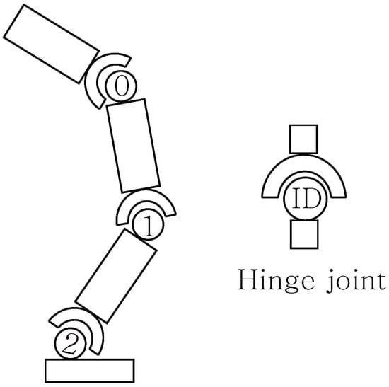
Figure 1. The MuJoCo Hopper-v5 environment. The control object is a planar monopedal robot consisting of a torso and leg links connected by three active hinge joints (labeled 0, 1, and 2). The agent aims to hop forward as fast as possible by applying torques to these joints while maintaining balance.

Next, we construct a Cliffworld environment to interpret action selection and the corresponding explanations. The Cliffworld environment is deliberately simple, allowing humans to readily infer both the approximate optimal action and its underlying rationale. This enables us to assess whether the explanations produced by RAISE align with human intuition. The objective in Cliffworld is for a robot to reach a goal. The goal $({\mathrm{goal}}_x,{\mathrm{goal}}_y)$ is situated between two cliffs. Figure 2 illustrates the map of the Cliffworld environment.

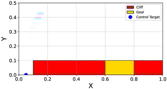
Figure 2. The Continuous CliffWorld environment. The agent, modeled as a point mass, starts at the initial position (blue marker) and aims to reach the goal region (yellow area) while avoiding the cliff regions (red areas). The environment is designed to evaluate the agent’s ability to balance safety (cliff avoidance) and efficiency (path minimization) under continuous state and action spaces.

The state and action are defined as

$$\mathbf{s}=(x,y,\dot{x},\dot{y}),\mathbf{a}=(F_x,F_y),$$

where $(x,y)$ represents the position of the object, $(\dot{x},\dot{y})$ denotes the velocity, and $(F_x,F_y)$ represents the forces applied in the horizontal and vertical directions, respectively.

The controlled object is governed by a damped point-mass model with mass m, friction coefficient $\mu$, and time step $\Delta t$. For state ${\mathbf{s}}_t$ and action ${\mathbf{a}}_t$, the velocity is updated including a linear damping term:

$${\dot{x}}_{t+1}={\dot{x}}_t+\Delta t{F}_{x,t}-\mu {\dot{x}}_t,{\dot{y}}_{t+1}={\dot{y}}_t+\Delta t{F}_{y,t}-\mu {\dot{y}}_t.$$

Subsequently, the position is updated as follows:

$$x_{t+1}=x_t+\Delta t{\dot{x}}_{t+1},y_{t+1}=y_t+\Delta t{\dot{y}}_{t+1}.$$

The reward is decomposed into three semantically interpretable components:

$$\overrightarrow{r}=\left(r_{\mathrm{cliff}},r_{\mathrm{goal}},r_{\mathrm{dist}}\right).$$

Here, $r_{\mathrm{cliff}}$ relates to entering (or avoiding) the cliff region, providing a reward of $-150$ if the agent falls. $r_{\mathrm{goal}}$ relates to reaching the goal, providing a reward of $+20$ upon arrival. $r_{\mathrm{dist}}$ represents a penalty based on the distance to the goal, given by $-{\displaystyle \frac{1}{2}}{(x-{\mathrm{goal}}_x)}^2-{(y-{\mathrm{goal}}_y)}^2$ at each step. The rationale for employing this Cliffworld environment is that its simplicity allows humans to intuitively predict the desirable action in each state to a certain extent. This facilitates the manual evaluation of the validity of the explanations generated by the system.

The policies evaluated in the experiments were trained using three algorithms: DDPG, AR-DDPG, and DRNR-DDPG. The hyperparameters utilized for training are presented in Table 2. For AR-DDPG and DRNR-DDPG, the disturbance parameter $\alpha$ is fixed at $0.1$. The value $\alpha =0.1$ is chosen because it is a standard setting commonly used in experiments across various studies utilizing the NR-MDP framework [14,15]. For clarity, the Algorithm 1 describes updates after each environment interaction. In our implementation, we instead apply the same update schedule every 50 environment steps: after collecting 50 transitions, we perform 50 protagonist updates and 50 adversary updates. All methods were trained for 1 million time steps under identical conditions. Each experiment was repeated using 10 different random seeds, and we report the average episode rewards, along with representative trajectories and examples of generated explanations.

Table 2. Hyperparameters used for training policies in DDPG, AR-DDPG, and DRNR-DDPG.

	DDPG	AR-DDPG	DRNR-DDPG
Update ratio (Prota & anta)	-	1:1	1:1
$\alpha$	-	0.1	0.1
Actor learning rate	$1\times {10}^{-4}$	$1\times {10}^{-4}$	$1\times {10}^{-4}$
Critic learning rate	$5\times {10}^{-4}$	$5\times {10}^{-4}$	$5\times {10}^{-4}$
$\gamma$	0.99	0.99	0.99
Batch size	128	128	128

5.2. Experiment 1: Robustness to Unseen Environment Parameters

5.2.1. Methodology and Settings

In this experiment, we verify whether the proposed method can maintain robust performance comparable to conventional action-robust reinforcement learning. We conduct a comparison among three methods: DDPG, AR-DDPG, and DRNR-DDPG.

During testing, returns were measured while varying the mass and friction coefficient of the controlled object relative to their values during training. Specifically, each environmental parameter was scaled from $0.1\times$ the training value up to a range where control performance significantly degrades. This range was discretized into 11 points. Consequently, returns were measured across a total of 121 environmental configurations. With the exception of the case where both mass and friction multipliers are $1.0\times$, all configurations represent environments not encountered during training. We calculated the average sum of rewards for all test parameter settings and present the results as heatmaps. For each environmental setting, evaluations were conducted over 10 episodes across 10 distinct random seeds. Additionally, we computed the average return across all 121 test environments for each method.

Finally, we outline the procedure used to select the specific policy checkpoints employed in this experiment. In the case of DDPG, since the control performance during training increased steadily and converged to a specific return value, we established this return as the threshold for evaluating robust performance. During training, policy models for each method were checkpointed every 2000 steps. We generated heatmaps for each checkpointed policy and selected the policy that achieved control performance exceeding the threshold in the largest number of environmental configurations for use in this experiment.

5.2.2. Results and Discussion

The experimental results are presented in Figure 3 and Table 3. From Figure 3, it is evident that DDPG exhibits the worst robust performance. Conversely, it is observed that the robust performance (indicated by the bright regions) of the policies trained with AR-DDPG and DRNR-DDPG is similar. Furthermore, as demonstrated in Table 3, which summarizes the average returns for each heatmap, DDPG shows inferior robust performance compared to the other methods, whereas AR-DDPG and DRNR-DDPG exhibit comparable values. This trend was consistently observed across all three environments employed in the experiments. This result is likely attributable to the fact that, as discussed in the proposed methodology, the optimal protagonist policies for both frameworks are theoretically identical; thus, policies with similar robust performance profiles were learned.

Figure 3. Comparison of DDPG, AR-DDPG, and the proposed method in situations where the test environment is different from the training environment. The maximum scale of the heatmap is capped at return achieved by DDPG during training.

Table 3. Average returns across 121 environmental configurations for each method.

	DDPG	AR-DDPG	DRNR-DDPG
Swimmer	86.5	104.7	98.6
Hopper	946.9	1216.4	1325.2
Walker2d	911.2	1244.9	1184.3

However, it was also noted that the shapes of the high-performance regions (bright areas) are not perfectly identical. We attribute this discrepancy to the fact that AR-DDPG and DRNR-DDPG do not yield exact optimal solutions for the NR-MDP and DRNR-MDP, respectively, but rather approximate solutions. Indeed, it has been proven that AR-DDPG does not guarantee convergence to the optimal solution of the max-min optimization problem [14]. Since DRNR-DDPG inherits the fundamental properties of AR-DDPG, it similarly fails to guarantee the exact optimal solution. Consequently, both methods obtain only approximate optimal solutions rather than the exact optima [14], which explains why the high-performance regions in the heatmaps do not perfectly overlap.

5.3. Experiment 2: Qualitative Evaluation of Explanation Validity via Case Studies

5.3.1. Methodology and Settings

In this experiment, we qualitatively evaluate whether the explanations generated by the proposed method, RAISE, align with the design intent of the environment. For evaluation, we employ the Continuous CliffWorld environment, which is intuitively interpretable for humans, and the MuJoCo Hopper environment, a high-dimensional continuous control task.

The objective of the experiment is to verify whether the system can present valid reward components as the rationale for the question “Why choose action $\mathbf{a}$ instead of action $\mathbf{b}$?” by comparing the optimal action $\mathbf{a}$ selected by the robust policy ${\pi }^R$ (trained via DRNR-DDPG) and the action $\mathbf{b}$ selected by the naive policy ${\pi }^N$ (trained via standard DDPG).

Setup in Continuous CliffWorld: In this environment, the agent aims to reach the goal while avoiding the Cliff. The reward function is decomposed into three components: $\overrightarrow{r}=(r_{\mathrm{cliff}},r_{\mathrm{goal}},r_{\mathrm{dist}})$. To verify the validity of the explanations, we perform a comparative analysis of the trajectories generated by ${\pi }^R$ and ${\pi }^N$. Specifically, we sample state $\mathbf{s}$ at the following three key points along the trajectories of ${\pi }^R$ and ${\pi }^R$, and evaluate the generated explanations:

• Initial state (${\mathbf{s}}_{\mathrm{start}}$): The starting point of the agent ($0.05,0,0,0$).
• Intermediate state (${\mathbf{s}}_{\mathrm{mid}}$): The state passed by each policy near the midpoint to the goal ($x\approx 0.3$). (${\mathbf{s}}_{\mathrm{mid}}^R=(0.28,0.16,0.56,-0.13)$, ${\mathbf{s}}_{\mathrm{mid}}^N=(0.28,0.12,0.46,-0.07)$).
• Near-terminal state (${\mathbf{s}}_{\mathrm{end}}$): The state preceding the goal area ($x\approx 0.6$). (${\mathbf{s}}_{\mathrm{end}}^R=(0.54,0.11,0.71,0.1)$, ${\mathbf{s}}_{\mathrm{end}}^N=(0.55,0.10,0.43,-0.012)$).

At each state $\mathbf{s}$, we estimate ${\overrightarrow{\Delta }}_c(\mathbf{s};\mathbf{a},\mathbf{b})$ according to Equation (2) using a trained Q-function, where $\mathbf{a}={\pi }^R\left(\mathbf{s}\right)$ and $\mathbf{b}={\pi }^N\left(\mathbf{s}\right)$, while fixing ${\mathbf{a}}^A={\pi }^{A\ast }\left(\mathbf{s}\right)$ as the worst-case adversarial action predicted by the trained adversary. Subsequently, based on the concept of Minimal Sufficient Explanations (MSX), the dominant reward components that constitute the rationale for preferring action $\mathbf{a}$ over $\mathbf{b}$ are extracted.

Furthermore, to demonstrate the necessity of accounting for adversarial disturbances, we compute ${\overrightarrow{\Delta }}^{\mathrm{Naive}}$ under the assumption that no adversarial disturbance is present:

$${\overrightarrow{\Delta }}^{\mathrm{Naive}}(\mathbf{s};\mathbf{a},\mathbf{b})={\displaystyle \frac{(\overrightarrow{Q}(\mathbf{s},\mathbf{a})-\overrightarrow{Q}(\mathbf{s},\mathbf{b}))}{{\sum }_{c\in \mathcal{C}}|{\overrightarrow{Q}}_c(\mathbf{s},\mathbf{a})-{\overrightarrow{Q}}_c(\mathbf{s},\mathbf{b})|}}$$

and perform a comparative analysis. Here, the Q-function is the action-value function learned by a DRNR-DDPG agent after sufficient training, identical to the one used to compute $\overrightarrow{\Delta }$. The pair of actions compared, $(\mathbf{a},\mathbf{b})$, remains identical to the previous setting.

Setup in MuJoCo Hopper: To verify the explanatory capability in a high-dimensional environment, we employ the Hopper-v5 environment. The objective of the Hopper task is to control a three-jointed robot to move as fast and as far as possible. The reward function consists of three components: forward reward (forward speed), control cost (energy efficiency), and healthy reward (fall avoidance). In the Hopper experiments, we evaluated the effectiveness of the explanations under a condition where the mass was increased by a factor of 2.0. Under this high-load environment with a $2.0\times$ mass increase, the naive policy (${\pi }^N$) failed to adapt to the changes in dynamics caused by the increased weight, resulting in episode failure due to falling (Unhealthy). Conversely, the robust policy (${\pi }^R$) successfully controlled the robot’s posture and maintained balance. We verify whether RAISE can explicitly capture the trade-off relationship in the state immediately preceding the fall of the naive policy. To this end, we initiated control from 5 random initial states and calculated the mean and standard deviation of the relative robust value difference $\overrightarrow{\Delta }(\mathbf{s};\mathbf{a},\mathbf{b})$ at the states immediately preceding the failure.

5.3.2. Results and Discussion

Case Study 1: Continuous CliffWorld. First, we discuss the comparative results of the trajectories in the Continuous CliffWorld environment. A comparison between the trajectory of the robust policy (${\pi }^R$) trained via DRNR-DDPG (Figure 4, left) and that of the naive policy (${\pi }^N$) trained via DDPG (Figure 4, right) reveals a distinct difference. The naive policy exhibits a tendency to move along the edge of the cliff region to reach the goal, thereby attempting to minimize the distance penalty ($r_{\mathrm{dist}}$). In contrast, the robust policy generates a trajectory that maintains a sufficient safety margin from the cliff. This aligns with the design intent, where the robust policy seeks to ensure safety against worst-case action disturbances through conservative behavior.

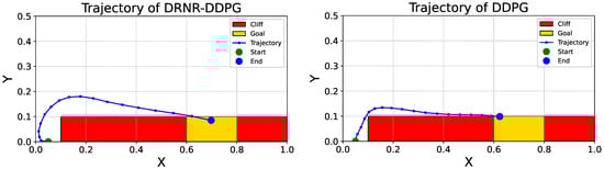
Figure 4. Trajectories in the Continuous CliffWorld environment generated by the robust policy trained with DRNR-DDPG (left) and the naive policy trained with DDPG (right). Red and yellow rectangles indicate the cliff and goal regions, respectively.

Next, we analyze the validity of the explanations generated by RAISE at several key states (${\mathbf{s}}_{\mathrm{start}},{\mathbf{s}}_{\mathrm{mid}}^N,{\mathbf{s}}_{\mathrm{mid}}^R,{\mathbf{s}}_{\mathrm{end}}^N,{\mathbf{s}}_{\mathrm{end}}^R$), based on Table 4.

Table 4. Quantitative analysis of explanations at key states in Continuous CliffWorld. The table reports the component-wise relative robust value differences $\overrightarrow{\Delta }$ for the cliff, goal, and distance components, calculated under the identified worst-case adversarial attack ${\mathbf{a}}^A$.

	${\overrightarrow{\mathbf{\Delta }}}_{\mathbf{cliff}}$	${\overrightarrow{\mathbf{\Delta }}}_{\mathbf{goal}}$	${\overrightarrow{\mathbf{\Delta }}}_{\mathbf{distance}}$	Worst Attack	Robust Action	Naive Action
${\mathbf{s}}_{\mathrm{start}}$	0.92	−0.07	−0.006	(1.0, −1.0)	(−1.0, −0.27)	(0.07, 1.0)
${\mathbf{s}}_{\mathrm{mid}}^N$	−0.27	0.66	0.07	(−1.0, 1.0)	(1.0, 0.96)	(0.48, −0.02)
${\mathbf{s}}_{\mathrm{mid}}^R$	0.31	0.61	0.08	(−1.0, 1.0)	(1.0, 0.05)	(0.86, −0.70)
${\mathbf{s}}_{\mathrm{end}}^N$	−0.14	0.75	0.10	(−1.0, 1.0)	(1.0, −0.15)	(0.26, −0.07)
${\mathbf{s}}_{\mathrm{end}}^R$	0.49	0.47	−0.04	(−1.0, 1.0)	(0.99, −0.58)	(−0.31, 0.85)

• Initial State (${\mathbf{s}}_{\mathrm{start}}$): At this point, the value of ${\overrightarrow{\Delta }}_{\mathrm{cliff}}$ is significantly large and positive ($0.92$), while ${\overrightarrow{\Delta }}_{\mathrm{goal}}$ and ${\overrightarrow{\Delta }}_{\mathrm{dist}}$ take negative or near-zero values. This suggests that the robust action was selected to reduce the risk of falling into the cliff (Safety component), even if it incurs slight losses in distance or goal-reaching speed. Based on this, RAISE generates the explanation “Considering the adversarial attack $(1,-1)$, to ensure safety ($r_{\mathrm{cliff}}$),” which accurately corresponds to the agent’s behavior of beginning to detour around the cliff.
• Intermediate State (${\mathbf{s}}_{\mathrm{mid}}^N$): At this point, ${\overrightarrow{\Delta }}_{\mathrm{cliff}}$ is negative at $-0.27$, whereas ${\overrightarrow{\Delta }}_{\mathrm{goal}}$ records a large positive value of $0.66$, and ${\overrightarrow{\Delta }}_{\mathrm{dist}}$ is $0.07$. This observation can be interpreted in two ways. First, the explanation may be incorrect: although the state is close to the cliff, the adversarial attack drives the agent away from the cliff region, and the agent therefore does not need to prioritize the cliff-related component. A probable cause for this failure to provide a correct explanation is that this state was not experienced during the training of the robust policy, rendering it an out-of-distribution (OOD) state. Second, the explanation may be correct: the worst-case disturbance can instead be viewed as preventing the agent from reaching the goal by acting against the distance-related component. In this case, the protagonist would focus on the goal component, since it must take actions that maximize the chance of reaching the goal despite the disturbance. In this case, RAISE explains that $\mathbf{a}$ was selected “Considering the adversarial attack $(-1,1)$, to ensure the goal ($r_{\mathrm{goal}}$).”
• Intermediate State (${\mathbf{s}}_{\mathrm{mid}}^R$): At the midpoint of the trajectory generated by the robust policy, the differences for all components (${\overrightarrow{\Delta }}_{\mathrm{cliff}},{\overrightarrow{\Delta }}_{\mathrm{goal}},{\overrightarrow{\Delta }}_{\mathrm{dist}}$) were positive. This indicates that in this state, the robust action is superior to the naive action in all aspects: safety, goal achievement, and distance reduction. In this case, prioritizing the simplicity of the explanation, RAISE explains that $\mathbf{a}$ was selected “Considering the adversarial attack $(-1,1)$, to ensure the goal ($r_{\mathrm{goal}}$).”
• Naive Policy Terminal State (${\mathbf{s}}_{\mathrm{end}}^N$): The analysis at the state immediately before the goal reached by the naive policy (${\mathbf{s}}_{\mathrm{end}}^N$) suggests an interesting trade-off. At this point, ${\overrightarrow{\Delta }}_{\mathrm{cliff}}$ is negative at $-0.14$, while ${\overrightarrow{\Delta }}_{\mathrm{goal}}$ records a very large positive value of $0.75$, and ${\overrightarrow{\Delta }}_{\mathrm{dist}}$ is $0.10$. This implies that while the naive action adheres to the shortest path until the very last moment, carrying the risk of goal failure upon disturbance occurrence, the robust action makes a choice that guarantees “certain goal achievement (${\overrightarrow{\Delta }}_{\mathrm{goal}}\gg 0$)” even if the margin against the cliff is slightly reduced (${\overrightarrow{\Delta }}_{\mathrm{cliff}}<0$). In other words, when goal achievement is imminent, “certainty of mission success” is prioritized over “excessive safety,” and RAISE presents the rationale: “Considering the adversarial attack $(-1,1)$, to ensure goal arrival ($r_{\mathrm{goal}}$).”
• Robust Policy Terminal State (${\mathbf{s}}_{\mathrm{end}}^R$): On the other hand, the situation differs at the terminal state reached by the robust policy itself (${\mathbf{s}}_{\mathrm{end}}^R$). Here, both ${\overrightarrow{\Delta }}_{\mathrm{cliff}}$ and ${\overrightarrow{\Delta }}_{\mathrm{goal}}$ are positive, with only ${\overrightarrow{\Delta }}_{\mathrm{dist}}$ being negative ($-0.04$). This indicates that because the robust agent maintained a distance from the cliff and approached safely from the beginning, it was capable of making a comfortable decision to “balance safety ($r_{\mathrm{cliff}}$) and goal achievement ($r_{\mathrm{goal}}$),” even if it meant sacrificing distance slightly at the final moment (${\overrightarrow{\Delta }}_{\mathrm{dist}}<0$). Also, for more concise explanations, RAISE explains that $\mathbf{a}$ was selected “Considering the adversarial attack (−1, 1), to ensure the goal (cliff).”

Finally, we examine how the generated explanations change in the absence of the worst-case disturbance (Table 5). Without the application of the worst-case disturbance, the explanations differ for all states except ${\mathbf{s}}_{\mathrm{start}}$ and ${\mathbf{s}}_{\mathrm{mid}}^N$. Specifically, for ${\mathbf{s}}_{\mathrm{mid}}^R$, the component prioritized by the agent shifts to the cliff component, while for ${\mathbf{s}}_{\mathrm{end}}^N$ and ${\mathbf{s}}_{\mathrm{end}}^R$, generating an explanation becomes impossible because $\overrightarrow{\Delta }$ becomes negative for all reward components, making the action choice unexplainable. This indicates that, if the adversary is ignored, DDPG action would be preferred at this state. These results demonstrate that accounting for adversarial disturbance is a crucial factor in the provision of valid explanations.

Table 5. Quantitative analysis of explanations at key states in Continuous CliffWorld when not considering adversarial attack.

	${\overrightarrow{\mathbf{\Delta }}}_{\mathbf{cliff}}^{\mathbf{Naive}}$	${\overrightarrow{\mathbf{\Delta }}}_{\mathbf{goal}}^{\mathbf{Naive}}$	${\overrightarrow{\mathbf{\Delta }}}_{\mathbf{distance}}^{\mathbf{Naive}}$
${\mathbf{s}}_{\mathrm{start}}$	0.75	−0.10	−0.14
${\mathbf{s}}_{\mathrm{mid}}^N$	−0.32	0.61	0.07
${\mathbf{s}}_{\mathrm{mid}}^R$	0.47	0.45	0.08
${\mathbf{s}}_{\mathrm{end}}^N$	−0.77	0.17	0.04
${\mathbf{s}}_{\mathrm{end}}^R$	−0.56	0.38	−0.04

The results presented above confirm that RAISE effectively identifies which reward components are prioritized depending on the specific situation and the worst-case disturbance. While it is considered that correct explanations were provided for states lying on the trajectory of the robust policy, explanations slightly deviating from the design intent were observed for states outside the robust policy’s trajectory.

Case Study 2: MuJoCo Hopper. In the high-dimensional Hopper environment, the evaluation of explanatory effectiveness focused on variations in environmental parameters, specifically a two-fold increase in mass. Experimental results demonstrated that under the high-load condition with the mass increased by a factor of $2.0$, the naive policy (${\pi }^N$) failed to adapt to the altered dynamics caused by the increased weight, resulting in a fall (Unhealthy outcome) mid-episode. Conversely, the robust policy (${\pi }^R$) successfully controlled the robot’s posture and maintained balance under the identical conditions.

In this scenario, the relative robust value difference $\overrightarrow{\Delta }$ calculated by RAISE clearly quantified the strategic divergence between the two policies:

• ${\overrightarrow{\Delta }}_{\mathrm{healthy}}\approx 0.78\pm 0.14$: The large positive value indicates that the robust action made a decisive contribution to survival (fall avoidance) against worst-case disturbance. The robust policy aims to preserve the future survival reward that the naive policy forfeits after falling.
• ${\overrightarrow{\Delta }}_{\mathrm{ctrl}\_\mathrm{cost}}\approx -0.04\pm 0.25$: The negative value implies that the robust agent sacrificed control cost (energy efficiency) compared to the naive agent. This is consistent with the physical context, where larger torque (control input) than usual was required to support the doubled mass and maintain balance.
• ${\overrightarrow{\Delta }}_{\mathrm{forward}}\approx -3\times {10}^{-3}\pm 3\times {10}^{-3}$: The difference regarding velocity is negligible, suggesting that it holds a lower priority compared to the criticality of survival.

In conclusion, RAISE characterized this situation as a trade-off, explaining that the agent selected high-output control to ensure survival (Healthy reward) by resisting the worst-case attack under increased mass, sacrificing energy efficiency (Control cost) while maintaining forward speed. For example, in one out of five trials, the following explanation was generated: the agent selected the DRNR-DDPG action (−0.98, 0.99, −1.0) instead of the DDPG action (−0.63, −0.49, −1.0) to secure the Healthy reward component under the worst-case disturbance (1, 1, 1). This demonstrates that RAISE correctly captures the design philosophy of robust control, which prioritizes safety (survival) over efficiency when facing unforeseen environmental changes (e.g., increased mass) and is capable of presenting it in a human-understandable format.

5.4. Experiment 3: Quantitative Analysis of Explanation Consistency and Stability

5.4.1. Methodology and Settings

Following the qualitative case analysis in the previous section, this experiment quantitatively verifies how statistically stable and consistent the explanations provided by the proposed framework are against state changes and counterfactual interventions. To this end, we adopt three approaches: (1) confirmation of intuitive consistency through the visualization of explanation maps, (2) stability evaluation using state sampling with action-noise mixture, and (3) regional explanation consistency analysis via counterfactual intervention.

Visualization of Explanation Maps: Prior to the quantitative analysis, we generate component-wise explanation maps to understand the distribution of explanations across states. Following the trajectories of the robust and naive policies in the Continuous Cliffworld, we visualize the most dominant reward component at each state by color to verify that the explanations exhibit consistent patterns near danger zones or goal regions. Here, for trajectory generation, we used $(1-\beta )\pi \left(\mathbf{s}\right)+\beta ϵ$, where $ϵ\sim \mathcal{U}\left({[-1,1]}^2\right)$ and $\beta =0.3$, for both $\pi ={\pi }^R$ and $\pi ={\pi }^N$. In addition, we plotted the trajectories using different colors according to the most dominant reward component at each state, $arg{max}_c{\overrightarrow{\Delta }}_c(\mathbf{s};{\pi }^R\left(\mathbf{s}\right),{\pi }^N\left(\mathbf{s}\right))$. In some cases, ${\sum }_c{\overrightarrow{\Delta }}_c(\mathbf{s};{\pi }^R\left(\mathbf{s}\right),{\pi }^N\left(\mathbf{s}\right))$ became negative, making $arg{max}_c{\overrightarrow{\Delta }}_c(\mathbf{s};{\pi }^R\left(\mathbf{s}\right),{\pi }^N\left(\mathbf{s}\right))$ undefined. We defined such cases as “none” and plotted them in gray. We plotted the trajectories from 30 episodes.

Stability Evaluation using Action-Noise Mixture: To evaluate the stability of the provided explanations, we assess the proportion of cases in which “none” is produced not only for states along trajectories generated by ${\pi }^R$, but also when the actions are perturbed by various disturbances, and we aim to identify the underlying cause of such “none” outputs. To this end, we injected uniformly distributed noise into the actions. This serves to verify whether appropriate explanations are consistently provided even under diverse environmental conditions. For the deterministic action of the robust policy ${\pi }^R$, we generate an action $u_{\beta }\left(\mathbf{s}\right)$ mixed with uniform noise $ϵ\sim \mathcal{U}\left({[-1,1]}^2\right)$ and execute rollouts:

$$u_{\beta }\left(\mathbf{s}\right)=(1-\beta ){\pi }^R\left(\mathbf{s}\right)+\beta ϵ.$$

Here, $\beta \in \{0.0,0.1,\dots ,0.5\}$ is a parameter adjusting the noise intensity. For the set of visited states ${\mathcal{S}}_{\beta }$ collected for each $\beta$ value, we calculate the sum of the relative robust value differences between the robust and naive actions, ${\sum }_{c\in \mathcal{C}}{\overrightarrow{\Delta }}_c\left(\mathbf{s}\right)$. We attributed the occurrence of “none” to the fact that the action values of the robust and naive actions are nearly identical. To identify cases where the relative robust value difference is close to 0 and determining superiority is difficult, we define the relative magnitude of the value difference as

$$\mathrm{Rel}(\mathbf{s};\mathbf{a},\mathbf{b})={\displaystyle \frac{{\sum }_{c\in \mathcal{C}}|{\overrightarrow{Q}}_c(\mathbf{s},m_{\alpha }(\mathbf{a},{\mathbf{a}}^A))-{\overrightarrow{Q}}_c(\mathbf{s},m_{\alpha }(\mathbf{b},{\mathbf{a}}^A))|}{{\sum }_{c\in \mathcal{C}}\left|{\overrightarrow{Q}}_c(\mathbf{s},m_{\alpha }(\mathbf{a},{\mathbf{a}}^A))\right|}}$$

and states satisfying $\mathrm{Rel}(\mathbf{s};\mathbf{a},\mathbf{b})\le 0.05$ are judged as a tie. In this experiment, we measure how the proportion of states where ${\sum }_c{\overrightarrow{\Delta }}_c<0$ (“none”) and the tie occurrence rate change as the noise intensity $\beta$ increases, analyzing how robustly the proposed method maintains explanations against changes in the state distribution.

For each $\beta$, we rolled out 30 episodes to collect states and computed: (i) the proportion of states satisfying ${\sum }_c{\overrightarrow{\Delta }}_c<0$; (ii) among those states, the proportion classified as “tie”; and (iii) the proportion satisfying ${\sum }_c{\overrightarrow{\Delta }}_c<0$ but not classified as “tie”. This allows us to quantitatively evaluate the relationship between “none” and “tie”.

Regional Consistency Analysis via Counterfactual Intervention: To verify whether explanations are generated consistently according to the geographical characteristics of the environment (danger region vs. goal region), we conduct a grid analysis targeting the region $0\le y\le 0.15$ (the lower area where the cliff and goal are adjacent) in Continuous CliffWorld. Specifically, we divide the environment along the x-axis into four sections (R1 $[0,0.1)$: near start, R2 $[0.1,0.6)$: above cliff, R3 $[0.6,0.8)$: above goal, R4 $[0.8,1.0)$: past goal). We discretized the x-axis interval $[0,1.0]$ into 80 bins and the y-axis interval $[0,0.15]$ into 20 bins, excluding the cliff and goal regions. At each state, we perform a counterfactual intervention by forcibly setting the y-axis action $F_y$ to $\{-1,+1\}$ while keeping the robust policy’s x-axis action $F_x$ fixed, and we compute the dominant reward component of $\overrightarrow{\Delta }\left(\mathbf{s}\right)$. All velocities were set to 0. The reason for setting $F_y$ as $-1$ and $+1$ is as follows:

• $F_y=-1$ (Movement towards the cliff): Since this is an action that invites danger, the cliff (safety) component should be extracted as the primary rationale.
• $F_y=+1$ (Movement away from the goal): Since this is an action that moves away from the goal, the goal component should be extracted as the primary rationale.

We plotted an explanation map of each state and quantitatively evaluated the ratio of dominant explanation components

$${\rho }_c={\displaystyle \frac{\left|\right\{\mathbf{s}|c={arg\; max}_{k\in \{\mathrm{cliff},\mathrm{dist},\mathrm{goal},\mathrm{none}\}}{\overrightarrow{\Delta }}_k\left(\mathbf{s}\right),\mathbf{s}\in {\mathcal{S}}_B\}|}{|{\mathcal{S}}_B|}},$$

where ${\mathcal{S}}_B$ = Set of state bins presented by RAISE in response to the intervention actions ($\pm 1$), which aligns with the intuitive hypotheses described above. In addition, we computed ${\tilde{\rho }}_c$, which represents the proportion excluding the effect of “none”.

5.4.2. Results and Discussion

Visual Inspection of Consistency: Prior to the statistical analysis, we present component-wise explanation maps along the trajectories in Continuous CliffWorld in Figure 5 to visually confirm the spatial distribution of explanation components.

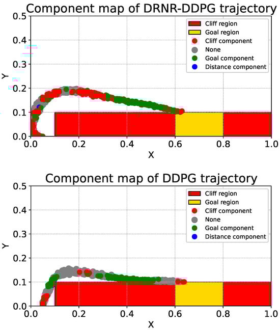
Figure 5. Component-wise explanation maps along the trajectories in Continuous CliffWorld ((top) DRNR-DDPG; (bottom) DDPG). Each visited state is colored by the dominant reward component according to the robust value difference ${\overrightarrow{\Delta }}_c(\mathbf{s};\mathbf{a},\mathbf{b})$ (cliff/goal/distance); “None” (gray) indicates that no component dominates (e.g., ties).

Referring to the upper panel of Figure 5, it is observed that the robust policy prioritizes the cliff component more than the naive policy in the interval $x\le 0.3$. This indicates a tendency to prioritize safety when distant from the goal. Conversely, the lower panel of Figure 5 shows a higher prevalence of “none” in the same interval. “none” regions (Gray regions) indicate areas where the naive policy’s action was judged to be superior to the robust action. In principle, we expect fewer gray regions along the robust trajectory; however, gray regions can still appear due to (i) OOD states, (ii) small value gaps between actions, and (iii) approximation errors in the learned value functions. Here, approximation errors may arise because DRNR-DDPG is a heuristic method for solving the DRNR-MDP, leading to the same issue observed in AR-DDPG [14]. The subsequent experiment suggests that many gray cases correspond to near-ties, indicating that the issue is often not a decisive preference reversal but rather negligible value differences amplified by approximation noise.

In the interval $x>0.3$, the focus shifts to the goal component, and immediately prior to goal arrival, the cliff component is prioritized again. This trend is consistent between the upper and lower panels of Figure 5. From this experiment, it was confirmed that explanation components are identical for spatially proximal states. However, it was also noted that there is a risk of incorrect explanations being provided if the state is not within the neighborhood of the robust policy’s trajectory.

Analysis of Stability against Action Perturbation: Table 6 reports how the proportion of “none” changes as noise is added to the actions, as well as the relationship between “none” and “tie”. First, no notable change was observed as $\beta$ increased from 0 to 0.4; however, when $\beta =0.5$, the proportion of “none” slightly increased. This is presumably because the accuracy of action-value estimation degrades for states that were rarely (or never) visited during training. Overall, across the tested values of $\beta$, the proportion of “none” remained between $35\%$ and $45\%$, which was higher than expected.

Table 6. Rates of negative total difference and tie cases across $\beta$.

$\mathit{\beta }$	Ratio of $({\sum }_{\mathit{c}}{\overrightarrow{\mathbf{\Delta }}}_{\mathit{c}}<0)$	Ratio of $(\mathbf{Tie}\mid {\sum }_{\mathit{c}}{\overrightarrow{\mathbf{\Delta }}}_{\mathit{c}}<0)$	Ratio of $({\sum }_{\mathit{c}}{\overrightarrow{\mathbf{\Delta }}}_{\mathit{c}}<0\wedge \neg \mathbf{Tie})$
0.0	38	70	11.4
0.1	40	79	8.4
0.2	38	85	5.7
0.3	35	83	6.0
0.4	37	85	5.6
0.5	45	85	6.8

To further analyze “none”, we focus on its relationship with “tie”. In fact, the conditional ratio $(\mathrm{tie}\mid {\sum }_c{\overrightarrow{\Delta }}_c<0)$ ranged from $70\%$ to $85\%$, indicating a strong association between “none” and “tie”. In other words, “none” does not necessarily indicate a failure of explanation; rather, it most often occurs when the action values of the robust and naive actions are nearly identical, in which case “none” is a justified outcome.

Analysis of Consistency via Counterfactual Interventions: Finally, to statistically corroborate the visual patterns we show Figure 6, and analyze the results of regional counterfactual interventions (Table 7).

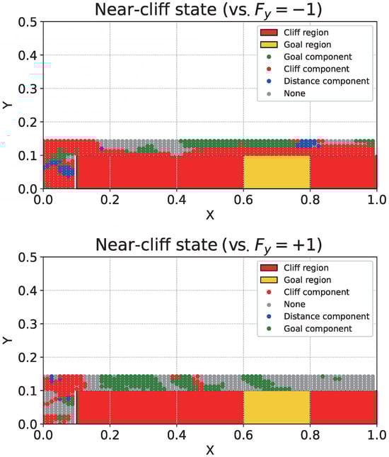
Figure 6. Component-wise explanation maps along the near-cliff states. Each state is colored by the dominant reward component according to the robust value difference ${\overrightarrow{\Delta }}_c(\mathbf{s};\mathbf{a},\mathbf{b})$ (cliff/goal/distance); “None” (gray) indicates that no component dominates (e.g., ties). The upper plot provides a component-wise explanation for the optimal action and for the case where we intervene by setting the y-component of the optimal action to −1. The lower plot provides a component-wise explanation for the optimal action and for the case where we intervene by setting the y-component of the optimal action to +1.

Table 7. Region-wise explanation statistics on a grid restricted to $0\le y\le 0.15$. We fix the robust policy’s $F_x$ and apply counterfactual interventions $F_y\in \{-1,+1\}$. For each x-region, we report (i) unconditional component ratios $p_c$ (including “none”), and (ii) conditional ratios ${\tilde{p}}_c$ computed after excluding “none” (i.e., normalized over explained states only).

Region	x-Range	${\mathit{F}}_{\mathit{y}}$	Unconditional Ratios ${\mathit{\rho }}_{\mathit{c}}$				Conditional Ratios ${\tilde{\mathit{\rho }}}_{\mathit{c}}$ (Exclude None)
			${\mathit{\rho }}_{\mathrm{cliff}}$	${\mathit{\rho }}_{\mathrm{dist}}$	${\mathit{\rho }}_{\mathrm{goal}}$	${\mathit{\rho }}_{\mathrm{none}}$	${\tilde{\mathit{\rho }}}_{\mathrm{cliff}}$	${\tilde{\mathit{\rho }}}_{\mathrm{dist}}$	${\tilde{\mathit{\rho }}}_{\mathrm{goal}}$
R1	$[0,0.1)$	$+1$	0.450	0.038	0.072	0.440	0.8036	0.0679	0.1286
		$-1$	0.670	0.140	0.140	0.050	0.7053	0.1474	0.1474
R2	$[0.1,0.6)$	$+1$	0.095	0.000	0.470	0.430	0.1667	0.0000	0.8246
		$-1$	0.390	0.004	0.230	0.370	0.6190	0.0063	0.3651
R3	$[0.6,0.8)$	$+1$	0.000	0.000	0.340	0.660	0.0000	0.0000	1.0000
		$-1$	0.530	0.080	0.380	0.000	0.5300	0.0800	0.3800
R4	$[0.8,1.0]$	$+1$	0.000	0.000	0.030	0.970	0.0000	0.0000	1.0000
		$-1$	0.650	0.063	0.073	0.200	0.8125	0.0788	0.0913

Looking at the upper panel of Figure 6 ($F_y=-1$), it is evident that the cliff component is prioritized in most of the $x<0.1$ interval. This is likely because, unless the agent crosses the edge of the cliff region, the action $F_y=-1$ plays the role of pushing the agent into the cliff region. Indeed, Table 7 shows that, in Region R1, the cliff component is highest (0.67) when $F_y=-1$, whereas it is relatively lower (0.45) when $F_y=+1$.

In the interval $x\ge 0.1$, the region $y\le 0.12$ prioritizes the cliff component, while the region above it focuses on “none” or “goal”. This is presumably because the agent is sufficiently distant from the cliff. In contrast, the lower panel of Figure 6 ($F_y=+1$) shows an increase in states focusing on the goal component even in the region $x\ge 0.1$ and $y\le 0.12$. This is because the region with $y\le 0.12$ is closer to the cliff and is therefore more likely to fall into the cliff under action perturbations. In contrast, when $y>0.12$, the agent does not immediately fall into the cliff even with action perturbations, and thus it is presumed to pay greater attention to the goal component. Moreover, the effect of the intervention is more clearly observed in Regions R2 and R3 in Table 7. In the R2 region located directly above the cliff, when an intervention towards the cliff ($F_y=-1$) was applied, the explanation ratio of the cliff component (${\tilde{\rho }}_{cliff}$) surged from $16.7\%$ (compared to $F_y=+1$) to $61.9\%$. This result aligns with the high density of red dots near the danger zone in Figure 6, indicating that the agent accurately recognizes the risk of falling. Furthermore, in the R3 (Above goal) region, when an intervention towards the goal direction ($F_y=+1$) was applied, the “goal” component appeared dominantly at $100\%$. This suggests that the action $F_y=1$ moves the agent away from the goal, implying that the immediate danger of falling into the cliff does not need to be the primary consideration.

Finally, in the interval $x>0.8$, when $F_y=-1$, the agent still focuses on the cliff component in the region $y\le 0.12$, whereas the proportion of none increases in the region $y>0.12$. In addition, when $F_y=+1$, none is output in most cases. This is presumably because $F_y=-1$ still acts to pull the agent toward the cliff. In contrast, under $F_y=+1$, the difference in action value is not substantial, and thus the explanation is likely to be none.

In conclusion, these results demonstrate that RAISE accurately grasps the context of the environment and is capable of providing consistent and stable explanations even in the face of state changes or hypothetical interventions.

5.5. Learning Time (Wall-Clock) Analysis

5.5.1. Methodology and Settings

In this experiment, we quantitatively analyze how the learning time (wall-clock time) changes as a function of the number of reward components $\left|\mathcal{C}\right|$. In particular, since we discussed that the computational overhead of our approach increases theoretically in proportion to $\left|\mathcal{C}\right|$ (Section 4.3), we empirically verify how varying $\left|\mathcal{C}\right|$ affects wall-clock learning time in our implementation by comparing against DR-DDPG. DR-DDPG is a DDPG-style baseline that implements the reward-decomposition idea of Juozapaitis et al. [17] for continuous action spaces, while our method additionally includes protagonist/adversary updates for robust learning.

We conducted experiments on two environments, Cliffworld and Hopper-v5, using the same hardware (CPU: Intel i9-12900K, GPU: NVIDIA RTX A6000) and the same training configuration (e.g., batch size, replay buffer, and network architectures). We measured learning time as the average wall-clock time (s) required to run 10,000 iterations executed after interacting with the environment once. To examine how learning time changes with the number of reward components, we varied $\left|\mathcal{C}\right|\in \{1,2,3\}$ and measured both DR-DDPG and our method under the same $\left|\mathcal{C}\right|$ condition. Since DRNR-DDPG with |C| = 1 is identical to AR-DDPG, we reuse the AR-DDPG measurement and report it in the ‘Ours (|C| = 1)’ row; therefore, we do not additionally run a separate experiment for this case.

5.5.2. Results and Discussion

Table 8 reports the learning time (s) as a function of $\left|\mathcal{C}\right|$. In both environments, the learning time increases as $\left|\mathcal{C}\right|$ increases, which is consistent with our discussion that critic updates scale linearly with the number of components.

Table 8. Wall-clock learning time (s) required to run 10,000 iterations (executed after one environment interaction) as a function of the number of reward components $\left|\mathcal{C}\right|$ on Cliffworld and Hopper-v5.

	Cliffworld			Hopper-v5
	$\mathcal{C}=\mathbf{1}$	$\mathcal{C}=\mathbf{2}$	$\mathcal{C}=\mathbf{3}$	$\mathcal{C}=\mathbf{1}$	$\mathcal{C}=\mathbf{2}$	$\mathcal{C}=\mathbf{3}$
DR-DDPG	0.033 s	0.045 s	0.055 s	20.19 s	25.27 s	30.25 s
Ours	0.071 s	0.091 s	0.112 s	37.89 s	48.1 s	58.44 s

In Cliffworld, DR-DDPG increases from 0.033 s at $\left|\mathcal{C}\right|=1$ to 0.055 s at $\left|\mathcal{C}\right|=3$, while our method increases from 0.071 s to 0.112 s. Similarly, in Hopper-v5, DR-DDPG increases from 20.19 s to 30.25 s, and our method increases from 37.89 s to 58.44 s as $\left|\mathcal{C}\right|$ goes from 1 to 3. Thus, the learning-time increase with respect to $\left|\mathcal{C}\right|$ is observed for both methods, and empirically exhibits an approximately linear trend.

Moreover, because our method performs additional adversary updates and related computations for robust learning, it consistently requires larger absolute wall-clock time than DR-DDPG for all $\left|\mathcal{C}\right|$ settings. For instance, in Hopper-v5, our method takes about $37.89/20.19\approx 1.88\times$ more time than DR-DDPG when $\left|\mathcal{C}\right|=1$ and about $58.44/30.25\approx 1.93\times$ more time when $\left|\mathcal{C}\right|=3$. These results support that the additional overhead of our method stems from (i) adversary-related computations required for robust learning and (ii) critic updates that scale proportionally to $\left|\mathcal{C}\right|$.

In summary, this experiment shows that (1) the wall-clock learning time increases with $\left|\mathcal{C}\right|$ in practice, (2) the absolute learning time of our method is larger than that of DR-DDPG due to robust-learning computations, while (3) the scaling trend with respect to $\left|\mathcal{C}\right|$ is similar for both methods. As future work, we will consider implementation options that further reduce wall-clock time, such as (a) a shared-backbone multi-head critic and (b) parallelizing the $\left|\mathcal{C}\right|$ critic updates.

6. Limitations

6.1. Explanation Coverage and Reliability (“None” Cases)

A notable fraction of states can return “none” explanations, which occurs when the estimated value difference between the candidate actions is near-tied or when approximation noise makes component-wise attribution unstable. As discussed in Table 6, most “none” outputs (70–85%) correspond to near-tie cases; therefore, the method returned “none” in those situations. In such cases, forcing a strong causal/credit assignment may lead to overconfident or misleading explanations. Therefore, our method conservatively abstains and outputs “none” as an uncertainty indicator. While this design improves reliability by avoiding potentially incorrect explanations, it can reduce explanation coverage from a user’s perspective, which may limit usability in scenarios requiring frequent explanations.

We believe that the occurrence of “none” can be mainly attributed to two reasons. First, in near-tie regions, “none” may be produced due to estimation errors of the learned Q-functions. Second, the value estimation can degrade for states that are rarely visited during training; i.e., out-of-distribution (OOD) states.

As future work, we plan to investigate techniques that stabilize the learned Q-functions (e.g., ensemble-based critics) to reduce approximation variance and thereby decrease the “none” rate without sacrificing reliability. In addition, to mitigate the OOD issue, a possible direction is to restrict the set of states for which explanations are provided to the neighborhood of states visited by the protagonist policy. Indeed, when qualitatively comparing the top panel of Figure 5 with Figure 6, the “none” cases appear to be relatively less prominent around the states visited by the protagonist policy. A more detailed investigation of this observation is an important direction for future work.

6.2. Assumption of Decomposable and Measurable Reward Components

Our framework assumes that the reward can be represented as an additive sum of semantically meaningful components, and that component signals are measurable or can be specified by the designer. This assumption is often reasonable in safety-critical domains (e.g., autonomous driving [27], finance portfolio [28]) where multiple operational metrics such as safety violations, energy usage, comfort, and productivity are explicitly defined and monitored. However, the assumption may not hold in settings with sparse rewards, delayed/unobservable rewards, or black-box reward models, where meaningful components cannot be directly defined or measured. In such cases, our theoretical guarantees no longer directly apply, and the applicability of the proposed explanation mechanism is limited. A practical extension to black-box rewards is to separate the optimization objective (black-box scalar reward) from explanation components by defining proxy component signals ${\left\{{\overrightarrow{r}}_c^D(\mathbf{s},\mathbf{a})\right\}}_{c\in \mathcal{C}}$ from measurable system logs/sensors (e.g., collision indicator, violation magnitude, energy/torque consumption, jerk), which may differ from the true reward, and then train corresponding explanatory critics ${\left\{{\overrightarrow{Q}}_c^D\right\}}_{c\in \mathcal{C}}$; however, the resulting explanations may not be fully aligned with the true optimization objective, and thus should be regarded as a post hoc/auxiliary explanation beyond the scope of our guarantees.

6.3. Computational Overhead for Component-Wise Critics

To provide component-level explanations, the proposed method maintains and updates critics that scale with the number of reward components $\left|\mathcal{C}\right|$. As discussed in Section 4.3, this yields an overhead that grows approximately linearly in $\left|\mathcal{C}\right|$ (primarily due to critic updates), which is also a structural characteristic shared with DR-DDPG [17]. While one can reduce overhead using a shared-backbone multi-head critic, such designs may introduce representation sharing that could weaken the independence of component-wise interpretations. Also, parallelizing the $\left|\mathcal{C}\right|$ critic updates may reduce training time. However, in this work, we adopt separate critics to keep component-level interpretations as disentangled as possible, and we leave a systematic study of the accuracy–efficiency trade-off as future work.

6.4. Evaluation Scope and Generalization

Our experiments are conducted on a limited set of MuJoCo continuous-control tasks under simulated disturbance models. Although these benchmarks are standard for evaluating continuous-control robustness, they do not cover the full diversity of real-world conditions, such as sensor noise, latency, unmodeled dynamics, or deployment constraints in physical systems. Therefore, the generalization of the proposed explanation framework to real-world robotics or autonomous driving systems remains to be validated. Future work includes evaluating on a broader set of continuous-control tasks, incorporating more realistic disturbance patterns, and validating on real-system logs or physical experiments.

7. Conclusions

In this study, to facilitate the application of reinforcement learning to safety-critical real-world environments, we proposed RAISE, a framework that simultaneously achieves high robustness and explainability within the Noisy Action Robust MDP (NR-MDP) framework. Furthermore, to implement this, we developed DRNR-DDPG, an algorithm that learns a robust policy alongside an action-value function possessing a decomposed reward structure.

Several experiments conducted to verify the effectiveness of the proposed method yielded the following insights:

First, we confirmed that DRNR-DDPG maintains robust performance comparable to existing robust reinforcement learning methods (e.g., AR-DDPG) while providing a rationale for action selection.

Second, through qualitative case studies (CliffWorld and Hopper), we demonstrated that the explanations generated by RAISE generally align with the physical characteristics and design intent of the environment. For instance, in the mass variation experiment (Mass $2.0\times$) within the MuJoCo Hopper environment, we revealed that the robust agent operates based on a clear trade-off: ensuring survival (Healthy reward) even at the expense of energy efficiency (Control cost). This indicates that the conservative behavior of robust policies, which are inherently black-box in nature, can be interpreted as human-understandable causal relationships.

Third, quantitative analyses employing Counterfactual Intervention and noise-mixture sampling corroborated that the proposed method provides statistically consistent explanations against state variations. In particular, the mechanism that isolates situations with similar action values as “ties”, thereby preventing the presentation of uncertain explanations, ensures reliability and represents a practically significant characteristic.

Future work includes extending the method to explicitly model uncertainty using techniques such as Distributional Reinforcement Learning, aiming to reduce regions classified as ties (explanation withholding) and to provide more precise explanations. Furthermore, as mentioned in the Limitations section, promising future directions include reducing approximation error by training the Q-function with an ensemble approach, and extending the framework to settings with black-box reward models. We also plan to further verify the practicality of the proposed framework through applications to more complex real-world tasks, such as autonomous driving and robotic control.

References

- Sutton, R.S.; Barto, A.G. Reinforcement Learning: An Introduction; The MIT Press: Cambridge, MA, USA, 1998. [Google Scholar]
- Kendall, A.; Hawke, J.; Janz, D.; Mazur, P.; Reda, D.; Allen, J.M.; Lam, V.D.; Bewley, A.; Shah, A. Learning to Drive in a Day. In Proceedings of the 2019 International Conference on Robotics and Automation (ICRA), Montreal, QC, Canada, 20–24 May 2019; pp. 8248–8254. [Google Scholar]
- Toromanoff, M.; Wirbel, E.; Moutarde, F. End-to-End Model-Free Reinforcement Learning for Urban Driving using Implicit Affordances. In Proceedings of the IEEE/CVF Conference on Computer Vision and Pattern Recognition, Seattle, WA, USA, 13–19 June 2020; pp. 7153–7162. [Google Scholar]
- Haarnoja, T.; Ha, S.; Zhou, A.; Tan, J.; Tucker, G.; Levine, S. Learning to walk via deep reinforcement learning. arXiv 2018, arXiv:1812.11103. [Google Scholar]
- Akkaya, I.; Andrychowicz, M.; Chociej, M.; Litwin, M.; McGrew, B.; Petron, A.; Paino, A.; Plappert, M.; Powell, G.; Ribas, R.; et al. Solving rubik’s cube with a robot hand. arXiv 2019, arXiv:1910.07113. [Google Scholar]
- Andrychowicz, O.M.; Baker, B.; Chociej, M.; Jozefowicz, R.; McGrew, B.; Pachocki, J.; Petron, A.; Plappert, M.; Powell, G.; Ray, A.; et al. Learning dexterous in-hand manipulation. Int. J. Robot. Res. 2020, 39, 3–20. [Google Scholar] [CrossRef]
- Gao, Q.; Schweidtmann, A.M. Deep reinforcement learning for process design: Review and perspective. Curr. Opin. Chem. Eng. 2024, 44, 101012. [Google Scholar] [CrossRef]
- Ho, K.H.; Cheng, J.Y.; Wu, J.H.; Chiang, F.; Chen, Y.C.; Wu, Y.Y.; Wu, I.C. Residual scheduling: A new reinforcement learning approach to solving job shop scheduling problem. IEEE Access 2024, 12, 14703–14718. [Google Scholar] [CrossRef]
- Bahrpeyma, F.; Reichelt, D. A review of the applications of multi-agent reinforcement learning in smart factories. Front. Robot. AI 2022, 9, 1027340. [Google Scholar] [CrossRef] [PubMed]
- Du, Y.; Liu, C.; Song, Y.; Li, Y.; Shen, Y. Rapid estimation of road friction for anti-skid autonomous driving. IEEE Trans. Intell. Transp. Syst. 2019, 21, 2461–2470. [Google Scholar] [CrossRef]
- Santini, S.; Albarella, N.; Arricale, V.M.; Brancati, R.; Sakhnevych, A. On-board road friction estimation technique for autonomous driving vehicle-following maneuvers. Appl. Sci. 2021, 11, 2197. [Google Scholar] [CrossRef]
- Pinto, L.; Davidson, J.; Sukthankar, R.; Gupta, A. Robust adversarial reinforcement learning. In Proceedings of the 34th International Conference on Machine Learning (ICML), Sydney, Australia, 6–11 August 2017; Volume 70, pp. 2817–2826. [Google Scholar]
- Zhang, H.; Chen, H.; Xiao, C.; Li, B.; Liu, M.; Boning, D.; Hsieh, C.J. Robust deep reinforcement learning against adversarial perturbations on state observations. Adv. Neural Inf. Process. Syst. 2020, 33, 21024–21037. [Google Scholar]
- Tessler, C.; Efroni, Y.; Mannor, S. Action Robust Reinforcement Learning and Applications in Continuous Control. In Proceedings of the 36th International Conference on Machine Learning (ICML), Long Beach, CA, USA, 9–15 June 2019; pp. 6215–6224. [Google Scholar]
- Kamalaruban, P.; Huang, Y.T.; Hsieh, Y.P.; Roll, P.; Shi, C.; Cevher, V. Robust reinforcement learning via adversarial training with langevin dynamics. Adv. Neural Inf. Process. Syst. 2020, 33, 8127–8138. [Google Scholar]
- Vinitsky, E.; Du, Y.; Parvate, K.; Jang, K.; Abbeel, P.; Bayen, A. Robust reinforcement learning using adversarial populations. arXiv 2020, arXiv:2008.01825. [Google Scholar] [CrossRef]
- Juozapaitis, Z.; Koul, A.; Fern, A.; Erwig, M.; Doshi-Velez, F. Explainable reinforcement learning via reward decomposition. In Proceedings of the IJCAI/ECAI Workshop on Explainable Artificial Intelligence, Macao, China, 11 August 2019. [Google Scholar]
- Madumal, P.; Miller, T.; Sonenberg, L.; Vetere, F. Explainable reinforcement learning through a causal lens. Proc. AAAI Conf. Artif. Intell. 2020, 34, 2493–2500. [Google Scholar] [CrossRef]
- Kim, S.; Shibuya, T. Explainable Reinforcement Learning via Causal Model Considering Agent’s Intention. In Proceedings of the IEEE International Conference on Systems, Man, and Cybernetics (SMC), Kuching, Malaysia, 6–10 October 2024; pp. 5391–5397. [Google Scholar]
- Tobin, J.; Fong, R.; Ray, A.; Schneider, J.; Zaremba, W.; Abbeel, P. Domain randomization for transferring deep neural networks from simulation to the real world. In Proceedings of the International Conference on Intelligent Robots and Systems (IROS), Vancouver, BC, Canada, 24–28 September 2017; pp. 23–30. [Google Scholar]
- Peng, X.B.; Andrychowicz, M.; Zaremba, W.; Abbeel, P. Sim-to-Real Transfer of Robotic Control with Dynamics Randomization. In Proceedings of the IEEE International Conference on Robotics and Automation (ICRA), Brisbane, Australia, 21–25 May 2018; pp. 3803–3810. [Google Scholar]
- Mehta, B.; Diaz, M.; Golemo, F.; Pal, C.J.; Paull, L. Active domain randomization. In Proceedings of the Conference on Robot Learning, Virtual, 16–18 November 2020; pp. 1162–1176. [Google Scholar]
- Wiesemann, W.; Kuhn, D.; Rustem, B. Robust Markov decision processes. Math. Oper. Res. 2013, 38, 153–183. [Google Scholar] [CrossRef]
- Heger, M. Consideration of risk in reinforcement learning. In Machine Learning Proceedings; Morgan Kaufmann: San Francisco, CA, USA, 1994; pp. 105–111. [Google Scholar]
- Bastani, O.; Pu, Y.; Solar-Lezama, A. Verifiable reinforcement learning via policy extraction. Adv. Neural Inf. Process. Syst. 2018, 31, 2494–2504. [Google Scholar]
- Verma, A.; Murali, V.; Singh, R.; Kohli, P.; Chaudhuri, S. Programmatically interpretable reinforcement learning. In Proceedings of the 35th International Conference on Machine Learning (ICML), Stockholm, Sweden, 10–15 July 2018; pp. 5045–5054. [Google Scholar]
- Ashwin, S.H.; Naveen Raj, R. Deep reinforcement learning for autonomous vehicles: Lane keep and overtaking scenarios with collision avoidance. Int. J. Inf. Technol. 2023, 15, 3541–3553. [Google Scholar] [CrossRef]
- Jiang, Y.; Olmo, J.; Atwi, M. Deep reinforcement learning for portfolio selection. Glob. Financ. J. 2024, 62, 101016. [Google Scholar] [CrossRef]
- Puterman, M.L. Markov Decision Processes: Discrete Stochastic Dynamic Programming; John Wiley & Sons: Hoboken, NJ, USA, 1994. [Google Scholar]
- Lillicrap, T.P.; Hunt, J.J.; Pritzel, A.; Heess, N.; Erez, T.; Tassa, Y.; Silver, D.; Wierstra, D. Continuous control with deep reinforcement learning. arXiv 2015, arXiv:1509.02971. [Google Scholar]
- Fujimoto, S.; Hoof, H.; Meger, D. Addressing function approximation error in actor-critic methods. In Proceedings of the International Conference on Machine Learning (ICML), Stockholm, Sweden, 10–15 July 2018; pp. 1587–1596. [Google Scholar]
Disclaimer/Publisher’s Note: The statements, opinions and data contained in all publications are solely those of the individual author(s) and contributor(s) and not of MDPI and/or the editor(s). MDPI and/or the editor(s) disclaim responsibility for any injury to people or property resulting from any ideas, methods, instructions or products referred to in the content. |
© 2026 by the authors. Licensee MDPI, Basel, Switzerland. This article is an open access article distributed under the terms and conditions of the Creative Commons Attribution (CC BY) license.