Communication-Efficient Asynchronous Fusion for Multi-Radar Systems via State and Covariance Projection

Abstract

Multi-radar systems can significantly improve tracking robustness and accuracy, but practical deployments are challenged by asynchronous sensing timestamps across distributed platforms and by limited communication bandwidth. This paper proposes a communication-efficient asynchronous track fusion framework based on state and covariance projection. Each radar performs local Kalman filtering and transmits only a compact track message consisting of the posterior state estimate, the associated error covariance, and a timestamp. At the fusion center, a causal reference time is chosen as the latest received timestamp, and all tracks are projected to this common time using a hybrid constant-acceleration (CA)/constant-velocity (CV) motion model with appropriately discretized process noise, followed by information-form (inverse-covariance) fusion. Under standard linear-Gaussian assumptions, the fusion rule is minimum mean square error (MMSE)-optimal when the projected estimation errors are approximately independent. We also analyze the computational complexity and the communication payload of the proposed procedure. Monte Carlo simulations with five heterogeneous radars and random inter-radar time offsets up to 37.5 ms over 100 runs show that the proposed fusion reduces the steady-state range root mean square error (RMSE) by about 66% and the radial-velocity RMSE by about 31% relative to the average single-radar tracker, while maintaining statistical consistency as verified by the normalized estimation error squared (NEES). These results indicate that projection-based track fusion provides an effective accuracy–communication trade-off for asynchronous multi-radar tracking.

1. Introduction

In modern surveillance and target tracking applications, particularly in highly dynamic environments, the use of multi-radar systems has become indispensable for achieving robust and high-precision situational awareness [1,2,3]. By integrating data from multiple geographically distributed sensors, these systems can overcome the limitations of single-radar platforms, such as restricted fields of view, measurement inaccuracies, and susceptibility to electronic countermeasures. The spatial diversity offered by a network of radars provides enhanced detection coverage, improved tracking accuracy, and greater resilience to sensor failures or target occlusion.

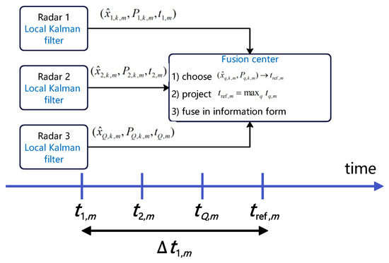
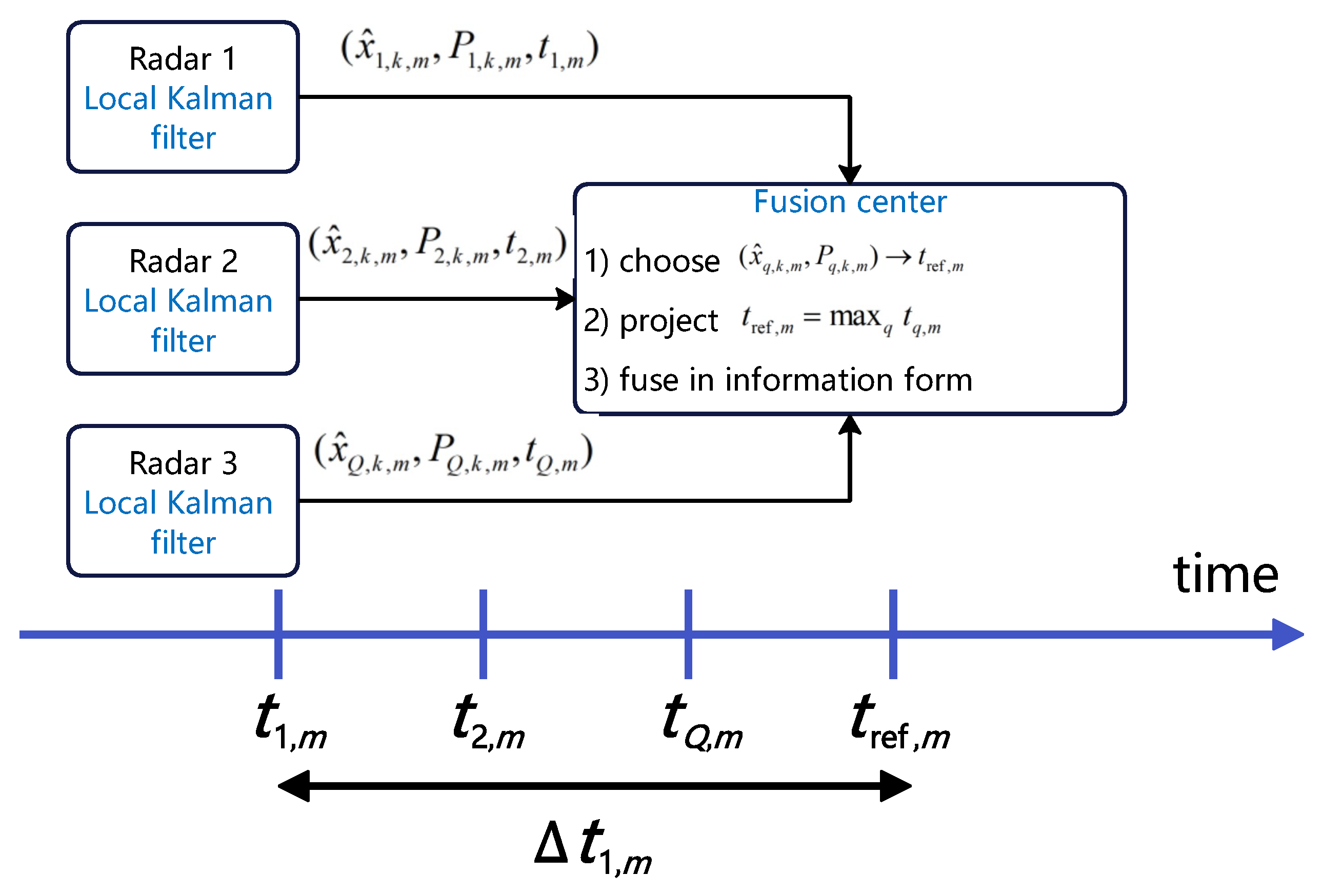
Despite these advantages, the effective fusion of data from multiple radars presents significant technical challenges. Two critical challenges include the inherent temporal asynchrony among radar platforms and the need to minimize communication overhead without degrading system functionality [4,5]. Asynchrony arises because distributed radars typically operate with independent clocks and scheduling protocols, leading to measurements being generated at different, uncoordinated time instants. If not properly handled, this temporal misalignment can lead to significant errors in state estimation, track divergence, and ultimately, a degradation of the overall system performance. Figure 1 illustrates the considered scenario and highlights the key entities and challenges: local radars run independent trackers and report compact track messages with timestamps, while the fusion center must align these asynchronous tracks to a common reference time before statistically sound fusion.

Figure 1. Scenario of asynchronous track-level fusion in a multi-radar network. Local radars generate posterior tracks at different timestamps $t_{q,m}$ and communicate compact track messages $({\widehat{\mathit{x}}}_{q,k,m},{\mathit{P}}_{q,k,m},t_{q,m})$. The fusion center selects the latest timestamp $t_{\mathrm{ref},m}$, projects each track forward by $\mathsf{\Delta }{\mathit{t}}_{q,m}$, and then fuses the aligned tracks in the information form.

To mitigate these issues, various fusion strategies have been developed. Centralized fusion, which processes raw data at a single node, offers theoretical optimality but is often infeasible due to its prohibitive communication bandwidth requirements. In contrast, distributed architectures reduce communication load by exchanging locally processed tracks, but they must address complex challenges such as track-to-track association and the fusion of correlated state estimates. While numerous methods have been proposed to handle temporal asynchrony, including measurement interpolation and state prediction, many introduce additional errors or lack statistical optimality. Furthermore, recent advancements in dual-functional radar-communication (DFRC) systems have primarily focused on embedding communication streams within radar waveforms, rather than addressing the specific problem of efficient, task-oriented information sharing for asynchronous state estimation in distributed networks. This leaves a critical gap in developing a framework that jointly optimizes tracking accuracy, communication efficiency, and robustness to asynchrony.

Furthermore, in tactical environments where communication bandwidth is often a scarce and constrained resource, transmitting raw sensor data from each radar to a central fusion center is frequently impractical. Such centralized approaches, while theoretically optimal, impose prohibitive communication loads that can saturate the network and introduce unacceptable latency, especially in high-speed scenarios involving multiple targets. This necessitates the development of communication-efficient fusion strategies that can operate effectively under strict bandwidth constraints.

This paper addresses these challenges by proposing a novel communication-efficient asynchronous fusion framework for multi-radar systems. Our approach leverages a state and covariance projection technique within a Kalman filtering framework to rigorously handle temporal asynchrony. By projecting local state estimates and their covariances to a common reference time, we enable a statistically optimal fusion process based on the minimum mean square error (MMSE) criterion under standard linear-Gaussian assumptions when the projected estimation errors are approximately independent. To address the communication bottleneck, our method relies on the exchange of processed, low-dimensional state information rather than high-bandwidth raw data. This paradigm balances the trade-off between estimation accuracy and communication cost, making it suitable for practical deployment.

The main contributions of this work are summarized as follows:

• We develop a novel asynchronous fusion Kalman filtering algorithm that provides a systematic framework for fusing processed radar state estimates from asynchronously operating sensors.
• We introduce a mathematically rigorous approach to address temporal synchronization by projecting local state estimates and covariance matrices to a unified reference time, ensuring statistically optimal fusion based on the MMSE criterion under standard linear-Gaussian assumptions when the projected estimation errors are approximately independent.
• We provide a comprehensive analysis of the algorithm’s computational complexity and communication efficiency, demonstrating its suitability for real-time implementation in high-speed radar applications.
• Through extensive Monte Carlo simulations with 100 independent runs, we demonstrate that our method achieves about 66% steady-state range root mean square error (RMSE) reduction and about 31% radial-velocity RMSE reduction relative to the average single-radar tracker, under up to 37.5 ms time asynchrony.
• We further provide ablation and sensitivity studies that quantify the impact of covariance projection, time asynchrony magnitude, and radar network size, strengthening the empirical evidence and reproducibility of the proposed framework.

The remainder of this paper is organized as follows. Section 2 reviews related work in the field. Section 3 presents the system model for the multi-radar system and target dynamics. Section 4 details the proposed asynchronous fusion Kalman filtering algorithm. Section 5 provides additional theoretical analysis of the proposed method. Section 6 provides a performance analysis of the algorithm. Simulation results are presented and discussed in Section 7, and Section 8 concludes the paper.

2. Related Work

The problem of data fusion in multi-sensor systems has been extensively studied, with numerous architectures and algorithms proposed to address diverse operational requirements. Fusion architectures are generally categorized as centralized, decentralized, or distributed (hierarchical) [6,7,8,9]. In a centralized architecture, raw measurements from all sensors are transmitted to a central processing node for fusion. This approach can achieve optimal performance as it utilizes all available information, but its requirement for high communication bandwidth often makes it impractical for systems with constrained network resources [10,11,12,13]. Decentralized architectures, in contrast, lack a central fusion node; instead, sensors communicate directly to iteratively fuse information. While highly robust, they can suffer from issues like data incest and increased computational load on each sensor. Distributed fusion offers a practical compromise, where local sensors first process their raw data to obtain state estimates (tracks) [14], which are then sent to a fusion center. This significantly reduces the communication overhead compared to centralized systems. However, distributed fusion must contend with challenges such as track-to-track association and the fusion of correlated estimates, which can arise if local tracks share common prior information [15,16,17,18]. Our work adopts a distributed architecture to ensure communication efficiency.

The issue of temporal asynchrony is a major hurdle in distributed multi-sensor systems. Synchronous fusion algorithms, which assume all measurements are available simultaneously, are ill-suited for practical scenarios where sensors operate asynchronously or with varying update rates. Several techniques have been proposed to handle asynchrony. One common approach is measurement interpolation or extrapolation, where measurements are adjusted to a common time reference before fusion. However, these methods can introduce additional errors and may not be statistically optimal. A more rigorous approach involves state projection to a common reference time, where each sensor’s state estimate is propagated forward or backward in time using a dynamic model [19,20,21,22]. This state-space alignment forms the basis of our proposed method, as it provides a principled way to fuse information from different time instances. In addition, stochastic finite set (random finite set) theory has motivated advanced multi-target multi-sensor filters, such as the probability hypothesis density (PHD) and cardinalized PHD (CPHD) families (e.g., Gaussian-mixture PHD variants), that are particularly effective in cluttered environments and in scenarios with target births/deaths [22]. These methods typically operate at the measurement level (or on intensity/cardinality representations) and thus are not directly comparable to the track-message fusion setting considered in this paper, where communication is constrained to transmitting only compact track summaries (state, covariance, timestamp).

Simultaneously, dual-functional radar-communication (DFRC) systems have emerged as a key enabling technology for future integrated sensing and communication networks. Much of the research in DFRC has focused on designing waveforms that can simultaneously perform radar sensing and convey communication data, often with the goal of maximizing data rates or optimizing communication quality of service [19,23]. While innovative, these approaches typically focus on embedding general-purpose communication streams within radar emissions. In contrast, our work addresses a different paradigm where the information to be shared is the processed radar state estimate itself, specifically for the purpose of improving tracking performance. This focus on task-specific information exchange under asynchronous conditions is a key distinction from mainstream DFRC research, which has not adequately addressed the complexities of asynchronous state estimation in distributed radar networks. Our paper bridges this gap by proposing a fusion framework tailored for such scenarios.

In summary, while DFRC and integrated sensing and communication (ISAC) studies often emphasize waveform/beamforming co-design to convey generic bit streams, this paper focuses on task-oriented information sharing: exchanging only compact track messages (state, covariance, and timestamp) to improve asynchronous state estimation under bandwidth constraints. To further position our contribution, Table 1 provides a tabular comparison of representative works with respect to fusion level, asynchrony handling, communicated information, and key differences.

Table 1. Comparison with representative related works on multi-sensor fusion and asynchronous processing.

Reference	Fusion Level	Asynchrony Handling	Shared Information	Key Facts (Relative to This Paper)
Aeberhard et al. (2012) [18]	Track-to-track	Asynchronous sensor updates (title)	Track estimates in information-matrix form	Addresses track-to-track fusion with asynchronous sensors; our work emphasizes an explicit state and covariance projection to a common reference time (chosen causally as the latest timestamp) and highlights the role of the inflation term for consistency and delay-aware weighting.
Zhang et al. (2020) [11]	Multi-sensor fusion for detection	Asynchronous data fusion (title)	Multi-sensor data and features	Focuses on asynchronous fusion for target detection; our focus is communication-efficient track-level Kalman filtering and fusion, with explicit projection, complexity analysis, and extensive ablation and consistency evaluation.
Lindenmaier et al. (2025) [14]	Track-to-track	Not the central focus	Track state and covariance	Emphasizes robust and runtime-efficient track fusion in automotive perception; our work focuses on temporal misalignment and communication-efficient sharing under asynchrony among distributed radars.
Sanson et al. (2021) [17]	Cooperative tracking (orthogonal frequency-division multiplexing (OFDM) radar)	Not the central focus	Radar and communication information	Studies cooperative tracking leveraging radar and communication information; in contrast, we study task-oriented sharing of compact tracks (state, covariance, and timestamp) for asynchronous multi-radar fusion, rather than waveform-embedded general-purpose communications.
Wang et al. (2025) [19]	Survey	Not applicable	Not applicable	Provides a broad review of multi-modal fusion sensing and related ISAC and DFRC efforts; our work contributes a concrete and analyzable fusion algorithm tailored for asynchronous track-level fusion with quantified communication and computational costs.
This work	Track-level (distributed)	Forward projection to a common (latest) reference time	Posterior state estimate, error covariance, and timestamp	Provides causal reference-time selection, state and covariance projection, information-form fusion, and detailed computational and communication analysis validated by Monte Carlo simulations, ablation, consistency evaluation, and sensitivity studies.

3. System Model

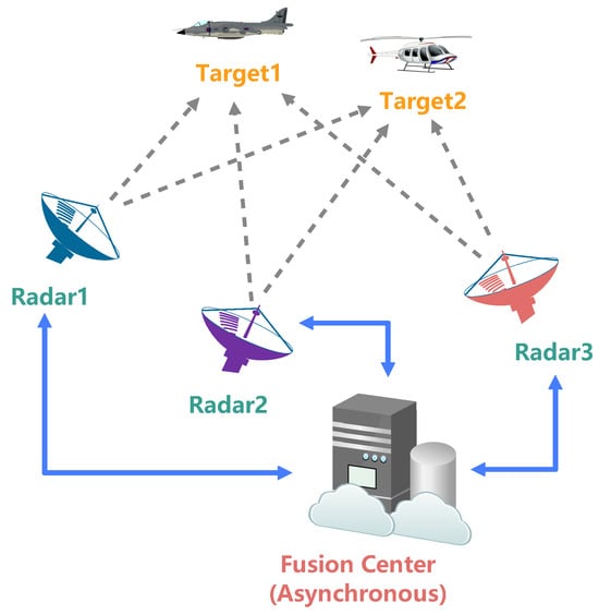
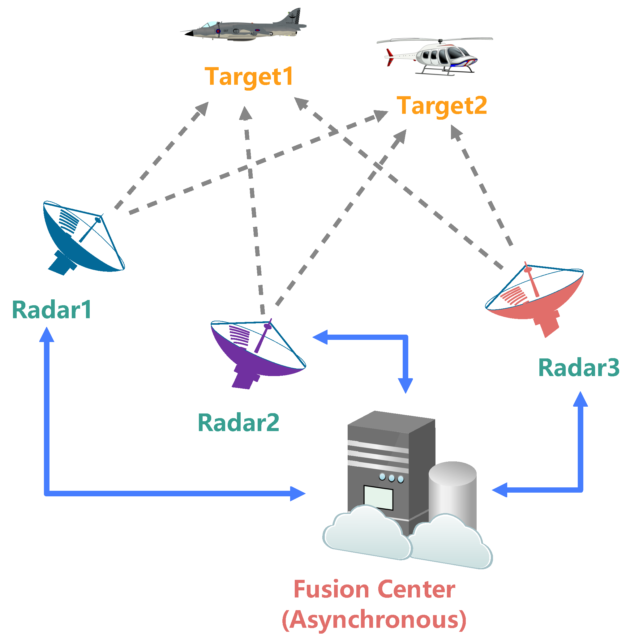
In this section, we define the mathematical framework for the multi-radar tracking system, including the target kinematic model and the radar measurement model. The overall system architecture is depicted in Figure 2, showing multiple radars observing targets and communicating processed information to a central fusion center. For clarity, Table 2 provides definitions of key symbols used throughout this paper.

Figure 2. A simplified and cleaner architecture of the multi-radar asynchronous fusion system. Dashed lines represent target detection signals. Solid blue lines indicate the communication of processed target information from local radars to the central fusion node. The fusion center outputs the final, fused target state.

Table 2. Nomenclature of key symbols used in this paper.

Symbol	Description
Q	Number of radars in the network.
K	Number of targets.
m	Fusion/update cycle index.
q	Radar index, $q\in \{0,\dots ,Q-1\}$.
k	Target index.
$t_{q,m}$	Local timestamp at radar q for cycle m.
$t_{\mathrm{ref},m}$	Reference time at fusion cycle m (chosen as $t_{\mathrm{ref},m}={max}_q{t}_{q,m}$).
$\mathsf{\Delta }{t}_{q,m}$	Non-negative time offset, $\mathsf{\Delta }{t}_{q,m}=t_{\mathrm{ref},m}-t_{q,m}\ge 0$.
${\mathit{x}}_{k,m}$	7D target state (range, radial velocity/acceleration, azimuth angle/rate, elevation angle/rate).
${\widehat{\mathit{x}}}_{q,k,m}$	Local posterior state estimate at radar q and time ${\mathit{t}}_{q,m}$.
${\mathit{P}}_{q,k,m}$	Local posterior error covariance of ${\widehat{\mathit{x}}}_{q,k,m}$.
$\mathit{F}\left(\mathsf{\Delta }t\right)$	State transition matrix over time step $\mathsf{\Delta }t$.
$\mathit{Q}\left(\mathsf{\Delta }t\right)$	Discretized process noise covariance over time step $\mathsf{\Delta }\mathit{t}$.
${\mathit{z}}_{q,k,m}$	Measurement vector (range, radial velocity, azimuth, elevation).
${\mathit{H}}_q$	Linear observation matrix mapping state to measurements.
${\mathit{R}}_{q,k,m}$	Measurement noise covariance.
${\mathit{K}}_{q,k,m}$	Kalman gain at radar q.
${\widehat{\mathit{x}}}_{f,k,m}$	Fused state estimate at the fusion center at time ${\mathit{t}}_{\mathrm{ref},m}$.
${\mathit{P}}_{f,k,m}$	Fused error covariance.
${\sigma }_a,{\sigma }_{{\alpha }_{\theta }},{\sigma }_{{\alpha }_{\varphi }}$	Process-noise standard deviations for radial and angular acceleration channels.
c	Speed of light.

3.1. Target Kinematic Model

To capture the full kinematic behavior of maneuvering targets, we employ a comprehensive 7-dimensional state vector for the k-th target at the m-th detection cycle:

$$\begin{array}{c}\hfill {\mathit{x}}_{k,m}={[r_{k,m},v_{k,m},a_{k,m},{\theta }_{k,m},{\omega }_{k,m},{\varphi }_{k,m},{\psi }_{k,m}]}^{\mathrm{T}},\end{array}$$

(1)

where $r_{k,m}$ is the range, $v_{k,m}$ is the radial velocity, $a_{k,m}$ is the radial acceleration, ${\theta }_{k,m}$ is the azimuth angle, ${\omega }_{k,m}$ is the azimuth angular velocity, ${\varphi }_{k,m}$ is the elevation angle, and ${\psi }_{k,m}$ is the elevation angular velocity.

The target motion is described by the following discrete-time linear state-space equation:

$$\begin{array}{c}\hfill {\mathit{x}}_{k,m+1}=\mathit{F}\left(T_p\right){\mathit{x}}_{k,m}+{\mathit{u}}_{k,m},\end{array}$$

(2)

where $T_p$ is the sampling interval between measurements at cycle m and $m+1$, $\mathit{F}\left(T_p\right)$ is the state transition matrix, and ${\mathit{u}}_{k,m}$ is the process noise. The process noise is modeled as a zero-mean Gaussian sequence with covariance matrix $\mathit{Q}\left(T_p\right)$, accounting for unmodeled dynamics and target maneuvers. For asynchronous updates, the covariance is discretized as a function of the actual time step $\mathsf{\Delta }t$, as detailed below.

We adopt a hybrid motion model that combines a constant-acceleration (CA) model for the radial dynamics with a constant-velocity (CV) model for the angular dynamics. This results in a block-diagonal state transition matrix:

$$\begin{array}{c}\hfill \mathit{F}\left(T_p\right)=\mathrm{diag}({\mathit{F}}_{CA}\left(T_p\right),{\mathit{F}}_{CV}\left(T_p\right),{\mathit{F}}_{CV}\left(T_p\right)),\end{array}$$

(3)

where the CA and CV blocks are given by

$${\mathit{F}}_{CA}\left(T_p\right)=\left[\begin{array}{ccc}1& T_p& 0.5T_p^2\\ 0& 1& T_p\\ 0& 0& 1\end{array}\right], {\mathit{F}}_{CV}\left(T_p\right)=\left[\begin{array}{cc}1& T_p\\ 0& 1\end{array}\right].$$

(4)

Discrete-Time Process Noise Covariance

To accommodate asynchronous sampling intervals and enable consistent state and covariance projection for arbitrary time offsets, we discretize the process noise covariance as a function of the time step $\mathsf{\Delta }t$. We assume that the radial acceleration a follows a random-walk model driven by a zero-mean Gaussian input $u_a$:

$$\begin{array}{c}\hfill a(t+\mathsf{\Delta }t)=a\left(t\right)+u_a,u_a\sim \mathcal{N}(0,{\sigma }_a^2),\end{array}$$

(5)

which yields the standard CA discrete covariance

$$\begin{array}{c}\hfill {\mathit{Q}}_{CA}\left(\mathsf{\Delta }t\right)={\sigma }_a^2{\mathit{g}}_r\left(\mathsf{\Delta }t\right){\mathit{g}}_r^{\mathrm{T}}\left(\mathsf{\Delta }t\right),{\mathit{g}}_r\left(\mathsf{\Delta }t\right)={[0.5\mathsf{\Delta }{t}^2,\mathsf{\Delta }t,1]}^{\mathrm{T}}.\end{array}$$

(6)

Similarly, for the angular CV channels, we model the angular velocities $(\omega ,\psi )$ as random walks driven by angular acceleration noises $u_{{\alpha }_{\theta }}\sim \mathcal{N}(0,{\sigma }_{{\alpha }_{\theta }}^2)$ and $u_{{\alpha }_{\varphi }}\sim \mathcal{N}(0,{\sigma }_{{\alpha }_{\varphi }}^2)$, which results in

$$\begin{array}{c}\hfill {\mathit{Q}}_{CV}(\mathsf{\Delta }t;{\sigma }_{\alpha })={\sigma }_{\alpha }^2{\mathit{g}}_{\theta }\left(\mathsf{\Delta }t\right){\mathit{g}}_{\theta }^{\mathrm{T}}\left(\mathsf{\Delta }t\right),{\mathit{g}}_{\theta }\left(\mathsf{\Delta }t\right)={[0.5\mathsf{\Delta }{t}^2,\mathsf{\Delta }t]}^{\mathrm{T}}.\end{array}$$

(7)

Therefore, the full 7D process noise covariance is block diagonal:

$$\begin{array}{c}\hfill \mathit{Q}\left(\mathsf{\Delta }t\right)=\mathrm{diag}\left({\mathit{Q}}_{CA}\left(\mathsf{\Delta }t\right),{\mathit{Q}}_{CV}(\mathsf{\Delta }t;{\sigma }_{{\alpha }_{\theta }}),{\mathit{Q}}_{CV}(\mathsf{\Delta }t;{\sigma }_{{\alpha }_{\varphi }})\right).\end{array}$$

(8)

Although (8) is derived under Gaussian driving-noise assumptions, in practice, $\mathit{Q}\left(\mathsf{\Delta }t\right)$ is often used as an effective uncertainty model that also accounts for residual unmodeled dynamics and possible model mismatch over the projection interval (e.g., abrupt maneuvers). To guard against underestimation under highly maneuverable targets, we adopt a conservative covariance inflation form

$$\begin{array}{c}\hfill {\mathit{Q}}_{\mathrm{eff}}\left(\mathsf{\Delta }t\right)=\kappa \mathit{Q}\left(\mathsf{\Delta }t\right),\kappa \ge 1,\end{array}$$

(9)

where $\kappa$ can be tuned based on the expected maneuver envelope or standard innovation-based consistency checks.

3.2. Radar Measurement Model

Each of the Q radars in the network transmits pulse signals $s_{q,m,n}\left(t\right)$ and processes the received echoes to observe the targets. The echo signal from the k-th target at the q-th radar is given by

$$\begin{array}{c}\hfill r_{q,m,k}\left(t\right)=\sum _{n=0}^{N-1}\sqrt{P_{r,q,k,m}}{s}_{q,m,n}(t-n{T}_p-t_{r,q,k,m}),\end{array}$$

(10)

where $t_{r,q,k,m}=2R_{q,k,m}/c$ is the round-trip propagation delay, $R_{q,k,m}$ denotes the propagation range between radar q and target k at time $t_{q,m}$, and $P_{r,q,k,m}$ is the received signal power determined by the standard radar equation:

$$\begin{array}{c}\hfill P_{r,q,k,m}={\displaystyle \frac{P_{t,q}{G}_{t,q}{G}_{r,q}{\lambda }_q^2{\sigma }_{q,k}}{{\left(4\pi \right)}^3{R}_{q,k,m}^4}},\end{array}$$

(11)

The total received signal at radar q is the sum of echoes from all K targets plus additive white Gaussian noise (AWGN) $w_{q,m}\left(t\right)$:

$$\begin{array}{c}\hfill r_{q,m}\left(t\right)=\sum _{k=0}^{K-1}{r}_{q,m,k}\left(t\right)+w_{q,m}\left(t\right).\end{array}$$

(12)

Through standard radar signal processing techniques (e.g., matched filtering, Doppler processing, and direction-of-arrival estimation), a measurement vector is extracted from $r_{q,m}\left(t\right)$ for each detected target.

The relationship between the target state and the measurement vector is described by the linear measurement equation:

$$\begin{array}{c}\hfill {\mathit{z}}_{q,k,m}={\mathit{H}}_q{\mathit{x}}_{k,m}+{\mathit{n}}_{q,k,m},\end{array}$$

(13)

where ${\mathit{n}}_{q,k,m}$ is the measurement noise, modeled as a zero-mean, white Gaussian sequence with covariance matrix ${\mathit{R}}_{q,k,m}$. The measurement vector ${\mathit{z}}_{q,k,m}$ consists of four direct observables:

$$\begin{array}{c}\hfill {\mathit{z}}_{q,k,m}={[{\widehat{r}}_{q,k,m},{\widehat{v}}_{q,k,m},{\widehat{\theta }}_{q,k,m},{\widehat{\varphi }}_{q,k,m}]}^{\mathrm{T}}.\end{array}$$

(14)

The measurement noise covariance is typically assumed diagonal, reflecting independent measurement errors in each channel:

$$\begin{array}{c}\hfill {\mathit{R}}_{q,k,m}=\mathrm{diag}({\sigma }_r^2,{\sigma }_v^2,{\sigma }_{\theta }^2,{\sigma }_{\varphi }^2).\end{array}$$

(15)

The observation matrix ${\mathit{H}}_q$ maps the 7-dimensional state space to the 4-dimensional measurement space:

$$\begin{array}{c}\hfill {\mathit{H}}_q=\left[\begin{array}{ccccccc}1& 0& 0& 0& 0& 0& 0\\ 0& 1& 0& 0& 0& 0& 0\\ 0& 0& 0& 1& 0& 0& 0\\ 0& 0& 0& 0& 0& 1& 0\end{array}\right].\end{array}$$

(16)

As detailed in Section 4, each radar processes its measurements locally to produce a state estimate ${\widehat{\mathit{x}}}_{q,k,m}$ and an associated covariance matrix ${\mathit{P}}_{q,k,m}$. To maintain communication efficiency, only this processed information is transmitted to the fusion center, rather than the raw echo data.

4. Asynchronous Radar Fusion Method

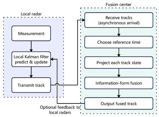
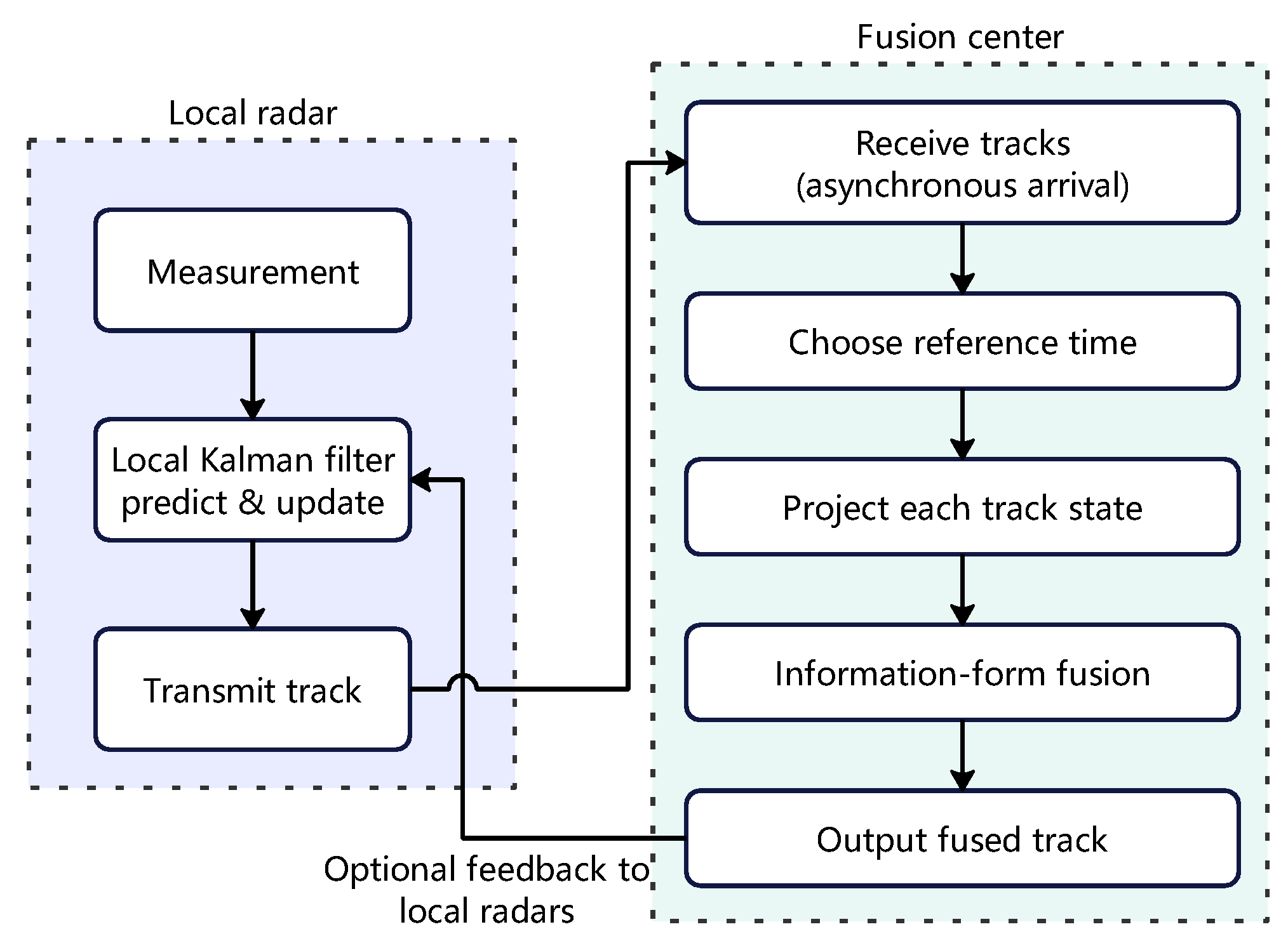
This section details our proposed asynchronous fusion algorithm for distributed multi-radar systems. The method comprises a two-stage process: first, each radar independently performs local target state estimation using standard Kalman filters; second, these asynchronous local estimates are sent to a fusion center. At the fusion center, a novel state and covariance projection technique is employed to align the estimates to a common reference time, followed by a statistically optimal fusion step (MMSE-optimal under standard linear-Gaussian assumptions when the projected estimation errors are approximately independent). This hierarchical approach ensures communication efficiency while rigorously addressing the challenge of temporal asynchrony. Figure 3 provides a detailed flowchart of the proposed framework, highlighting the key processing stages at local radars and at the fusion center.

Figure 3. Flowchart of the proposed communication-efficient asynchronous fusion framework. Each radar performs local Kalman filtering and sends compact track messages with timestamps. The fusion center selects a causal reference time, projects asynchronous tracks to this time, and fuses them in the information form.

4.1. Local Kalman Filtering

Each radar platform q maintains a local Kalman filter for each tracked target k. Upon acquiring a new measurement ${\mathit{z}}_{q,k,m}$ at its local time $t_{q,m}$, the radar updates its estimate of the target’s state vector ${\mathit{x}}_{k,m}$. The local filtering process consists of the standard prediction and update steps.

1.

Prediction: The state and covariance from the previous cycle $(m-1)$ are predicted forward to the current time $t_{q,m}$. Let $T_{q,m}=t_{q,m}-t_{q,m-1}$ be the local measurement interval.

$$\begin{array}{cc}\hfill {\widehat{\mathit{x}}}_{q,k,m|m-1}& =\mathit{F}\left(T_{q,m}\right){\widehat{\mathit{x}}}_{q,k,m-1}\hfill \end{array}$$

(17)

$$\begin{array}{cc}\hfill {\mathit{P}}_{q,k,m|m-1}& =\mathit{F}\left(T_{q,m}\right){\mathit{P}}_{q,k,m-1}\mathit{F}{\left(T_{q,m}\right)}^{\mathrm{T}}+\mathit{Q}\left(T_{q,m}\right)\hfill \end{array}$$

(18)

2.

Update: The predicted state is then corrected using the new measurement ${\mathit{z}}_{q,k,m}$.

$$\begin{array}{cc}\hfill {\mathit{K}}_{q,k,m}& ={\mathit{P}}_{q,k,m|m-1}{\mathit{H}}_q^{\mathrm{T}}{({\mathit{H}}_q{\mathit{P}}_{q,k,m|m-1}{\mathit{H}}_q^{\mathrm{T}}+{\mathit{R}}_{q,k,m})}^{-1}\hfill \end{array}$$

(19)

$$\begin{array}{cc}\hfill {\widehat{\mathit{x}}}_{q,k,m}& ={\widehat{\mathit{x}}}_{q,k,m|m-1}+{\mathit{K}}_{q,k,m}({\mathit{z}}_{q,k,m}-{\mathit{H}}_q{\widehat{\mathit{x}}}_{q,k,m|m-1})\hfill \end{array}$$

(20)

$$\begin{array}{cc}\hfill {\mathit{P}}_{q,k,m}& =(\mathit{I}-{\mathit{K}}_{q,k,m}{\mathit{H}}_q){\mathit{P}}_{q,k,m|m-1}{(\mathit{I}-{\mathit{K}}_{q,k,m}{\mathit{H}}_q)}^{\mathrm{T}}+{\mathit{K}}_{q,k,m}{\mathit{R}}_{q,k,m}{\mathit{K}}_{q,k,m}^{\mathrm{T}}\hfill \end{array}$$

(21)

Equation (21) adopts the Joseph stabilized form to better preserve symmetry and positive semidefiniteness of ${\mathit{P}}_{q,k,m}$ in numerical implementations. The output of this local processing is the local posterior state estimate ${\widehat{\mathit{x}}}_{q,k,m}$ and its associated error covariance matrix ${\mathit{P}}_{q,k,m}$, both valid at time $t_{q,m}$. This information is then transmitted to the fusion center.

4.2. Asynchronous Fusion via State and Covariance Projection

Given the lack of strict time synchronization, the local estimates $({\widehat{\mathit{x}}}_{q,k,m},{\mathit{P}}_{q,k,m})$ from different radars arrive at the fusion center corresponding to different time instants $t_{q,m}$. To address this, we propose an asynchronous fusion algorithm that achieves reliable and statistically sound state estimation despite temporal misalignment.

For each fusion cycle m, the fusion center designates a common reference time. To avoid non-causal backward projection (negative time offsets), we select the reference time as the latest timestamp among the received local tracks:

$$\begin{array}{c}\hfill t_{\mathrm{ref},m}=\underset{q\in {\mathcal{Q}}_m}{max}{t}_{q,m}.\end{array}$$

(22)

Here, ${\mathcal{Q}}_m$ denotes the set of radars whose track messages are available at fusion cycle m (e.g., under node addition/exit or packet loss); in the fully connected case, ${\mathcal{Q}}_m=\{0,\dots ,Q-1\}$. The non-negative time offset for radar q is then defined as $\mathsf{\Delta }{t}_{q,m}=t_{\mathrm{ref},m}-t_{q,m}\ge 0$ for $q\in {\mathcal{Q}}_m$. The asynchronous fusion procedure consists of the following steps:

1.

State Projection: For each radar q, its local state estimate ${\widehat{\mathit{x}}}_{q,k,m}$ is projected to the reference time $t_{\mathrm{ref},m}$ using the target motion model:

$$\begin{array}{c}\hfill {\widehat{\mathit{x}}}_{q,k,m|\mathrm{ref},m}=\mathit{F}\left(\mathsf{\Delta }{t}_{q,m}\right){\widehat{\mathit{x}}}_{q,k,m}\end{array}$$

(23)

where $\mathit{F}\left(\mathsf{\Delta }t\right)$ is the 7D transition matrix over $\mathsf{\Delta }t$, which follows the block-diagonal structure introduced in Section 3.1:

$$\begin{array}{c}\hfill \mathit{F}\left(\mathsf{\Delta }t\right)=\mathrm{diag}({\mathit{F}}_{CA}\left(\mathsf{\Delta }t\right),{\mathit{F}}_{CV}\left(\mathsf{\Delta }t\right),{\mathit{F}}_{CV}\left(\mathsf{\Delta }t\right)).\end{array}$$

(24)

2.

Covariance Projection: The corresponding error covariance matrix is projected to the same reference time, accounting for the process noise accumulated during the projection interval:

$$\begin{array}{cc}\hfill {\mathit{P}}_{q,k,m|\mathrm{ref},m}& =\mathit{F}\left(\mathsf{\Delta }{t}_{q,m}\right){\mathit{P}}_{q,k,m}\mathit{F}{\left(\mathsf{\Delta }{t}_{q,m}\right)}^{\mathrm{T}}\hfill \\ \hfill & +\mathit{Q}\left(\mathsf{\Delta }{t}_{q,m}\right)\hfill \end{array}$$

(25)

where $\mathit{Q}\left(\mathsf{\Delta }t\right)$ is given in (8). To mitigate potential model mismatch under highly maneuverable targets, we may use the conservative inflated covariance ${\mathit{Q}}_{\mathrm{eff}}\left(\mathsf{\Delta }t\right)=\kappa \mathit{Q}\left(\mathsf{\Delta }t\right)$ with $\kappa \ge 1$ as in (9). As proved in Section 5.1 (Equations (35)–(37)), the projection in (23)–(25) preserves unbiasedness and yields the correct second-order uncertainty at the reference time under the assumed linear-Gaussian dynamics in (32), which motivates our projection design (and explains why the additive $\mathit{Q}\left(\mathsf{\Delta }t\right)$ term is required for consistency). When the motion model is mismatched, the projected mean in (23) may become biased; ${\mathit{Q}}_{\mathrm{eff}}\left(\mathsf{\Delta }t\right)$ should be interpreted as an effective (conservative) uncertainty model that reduces the overconfident weighting of delayed tracks, but it does not correct model-induced bias.

3.

Data Fusion: With all local estimates and covariances aligned to the same reference time, they can be fused. Under the common assumption that the projected estimation errors are (approximately) uncorrelated across radars, the MMSE-optimal fusion rule is obtained by inverse-covariance weighting:

$$\begin{array}{c}\hfill {\mathit{P}}_{f,k,m}^{-1}=\sum _{q\in {\mathcal{Q}}_m}{\mathit{P}}_{q,k,m|\mathrm{ref},m}^{-1}\end{array}$$

(26)

$$\begin{array}{c}\hfill {\widehat{\mathit{x}}}_{f,k,m}={\mathit{P}}_{f,k,m}\sum _{q\in {\mathcal{Q}}_m}{\mathit{P}}_{q,k,m|\mathrm{ref},m}^{-1}{\widehat{\mathit{x}}}_{q,k,m|\mathrm{ref},m}\end{array}$$

(27)

where ${\widehat{\mathit{x}}}_{f,k,m}$ and ${\mathit{P}}_{f,k,m}$ are the final fused state estimate and covariance for the k-th target at the reference time $t_{\mathrm{ref},m}$. The fused estimate can be used as the prior for the next fusion cycle or disseminated back to local radars to improve subsequent tracking performance. Moreover, Section 5.3 (Equation (40)) establishes the covariance-ordering property of information-form fusion under the independence assumption, i.e., ${\mathit{P}}_{f,k,m}⪯{\mathit{P}}_{q,k,m|\mathrm{ref},m}$ for all q; this property is a direct theoretical basis for using (26) and (27) in the method design. Section 5.2 further interprets how $\mathit{Q}\left(\mathsf{\Delta }t\right)$ induces a principled delay-aware down-weighting of more asynchronous tracks. We emphasize that the MMSE optimality of (26) and (27) hinges on the correctness of the assumed projection/fusion model and the approximate independence of projected errors; under strong model mismatch or unknown cross-correlations, conservative alternatives (e.g., CI) and/or additional inflation/gating are preferred to avoid overconfident fusion.

4.2.1. MMSE Optimality and Information-Form Interpretation

Equations (26) and (27) can be interpreted in the information form and are MMSE-optimal under standard Gaussian assumptions. When the projection model is mismatched (or when projected errors are cross-correlated), these assumptions may not strictly hold; in that case, we interpret (26) and (27) as a practical information-weighted fusion rule and use conservative uncertainty modeling (e.g., ${\mathit{Q}}_{\mathrm{eff}}$, CI) to preserve consistency. Let the projected estimates at the reference time be

$$\begin{array}{c}\hfill {\widehat{\mathit{x}}}_{q,k,m|\mathrm{ref},m}={\mathit{x}}_{k,m}+{\mathit{e}}_{q,k,m},{\mathit{e}}_{q,k,m}\sim \mathcal{N}(\mathbf{0},{\mathit{P}}_{q,k,m|\mathrm{ref},m}),\end{array}$$

(28)

and assume ${\mathit{e}}_{q,k,m}$ are mutually independent across q. Then, the product of Gaussian likelihoods yields a Gaussian posterior whose information matrix and information vector satisfy

$$\begin{array}{cc}\hfill {\mathit{Y}}_{f,k,m}& =\sum _{q\in {\mathcal{Q}}_m}{\mathit{Y}}_{q,k,m},{\mathit{Y}}_{q,k,m}={\mathit{P}}_{q,k,m|\mathrm{ref},m}^{-1},\hfill \end{array}$$

(29)

$$\begin{array}{cc}\hfill {\mathit{y}}_{f,k,m}& =\sum _{q\in {\mathcal{Q}}_m}{\mathit{y}}_{q,k,m},{\mathit{y}}_{q,k,m}={\mathit{Y}}_{q,k,m}{\widehat{\mathit{x}}}_{q,k,m|\mathrm{ref},m},\hfill \end{array}$$

(30)

and the fused estimate is ${\widehat{\mathit{x}}}_{f,k,m}={\mathit{Y}}_{f,k,m}^{-1}{\mathit{y}}_{f,k,m}$, which is equivalent to (26) and (27).

4.2.2. Robust Fusion Under Unknown Cross-Correlations

In track-to-track fusion, local estimates may become cross-correlated due to common priors, feedback, or shared modeling assumptions. In such cases, naive inverse-covariance fusion can underestimate uncertainty (data incest). A conservative and widely used alternative is covariance intersection (CI), which fuses information using weights $\left\{{\omega }_q\right\}$ satisfying ${\omega }_q\ge 0$ and ${\sum }_{q\in {\mathcal{Q}}_m}{\omega }_q=1$:

$$\begin{array}{c}\hfill {\mathit{P}}_{f,k,m}^{-1}=\sum _{q\in {\mathcal{Q}}_m}{\omega }_q{\mathit{P}}_{q,k,m|\mathrm{ref},m}^{-1},{\widehat{\mathit{x}}}_{f,k,m}={\mathit{P}}_{f,k,m}\sum _{q\in {\mathcal{Q}}_m}{\omega }_q{\mathit{P}}_{q,k,m|\mathrm{ref},m}^{-1}{\widehat{\mathit{x}}}_{q,k,m|\mathrm{ref},m}.\end{array}$$

(31)

The weights can be chosen to minimize a scalar objective such as $\mathrm{tr}\left({\mathit{P}}_{f,k,m}\right)$ or $logdet\left({\mathit{P}}_{f,k,m}\right)$, providing robustness when cross-covariances are unknown or difficult to maintain.

4.3. Algorithm Summary and Initialization

The complete asynchronous fusion process is summarized in Algorithm 1. The algorithm operates recursively for each fusion cycle.

Algorithm 1 Asynchronous fusion Kalman filtering algorithm.

1: Input: Available local estimates $\left\{({\widehat{\mathit{x}}}_{q,k,m},{\mathit{P}}_{q,k,m})\right\}$ and timestamps $\left\{t_{q,m}\right\}$ for $q\in {\mathcal{Q}}_m$. 2: Output: Fused estimate $({\widehat{\mathit{x}}}_{f,k,m},{\mathit{P}}_{f,k,m})$. 3: Initialization: 4: Set reference time $t_{ref}\leftarrow {max}_{q\in {\mathcal{Q}}_m}{t}_{q,m}$, where ${\mathcal{Q}}_m$ is the set of available radars at cycle m. 5: Initialize fused covariance inverse: ${\mathit{P}}_{f,inv}\leftarrow \mathbf{0}$. 6: Initialize fused state sum: ${\widehat{\mathit{x}}}_{f,sum}\leftarrow \mathbf{0}$. 7: for each available radar $q\in {\mathcal{Q}}_m$ do 8:     Calculate time offset: $\mathsf{\Delta }t\leftarrow t_{ref}-t_{q,m}$. 9:     // Project state and covariance to reference time 10:     ${\widehat{\mathit{x}}}_{proj}\leftarrow \mathit{F}\left(\mathsf{\Delta }t\right){\widehat{\mathit{x}}}_{q,k,m}$. 11:     ${\mathit{P}}_{proj}\leftarrow \mathit{F}\left(\mathsf{\Delta }t\right){\mathit{P}}_{q,k,m}\mathit{F}{\left(\mathsf{\Delta }t\right)}^{\mathrm{T}}+\mathit{Q}\left(\mathsf{\Delta }t\right)$. 12:     // Accumulate for fusion 13:     ${\mathit{P}}_{f,inv}\leftarrow {\mathit{P}}_{f,inv}+{\mathit{P}}_{proj}^{-1}$. 14:     ${\widehat{\mathit{x}}}_{f,sum}\leftarrow {\widehat{\mathit{x}}}_{f,sum}+{\mathit{P}}_{proj}^{-1}{\widehat{\mathit{x}}}_{proj}$. 15: end for 16: // Compute final fused estimate 17: ${\mathit{P}}_{f,k,m}\leftarrow {\mathit{P}}_{f,inv}^{-1}$. 18: ${\widehat{\mathit{x}}}_{f,k,m}\leftarrow {\mathit{P}}_{f,k,m}{\widehat{\mathit{x}}}_{f,sum}$. 19: return$({\widehat{\mathit{x}}}_{f,k,m},{\mathit{P}}_{f,k,m})$.

Let d denote the state dimension ($d=7$ in this paper), Q the number of radars, and K the number of targets. For each target and each radar in Algorithm 1, the state projection ${\widehat{\mathit{x}}}_{proj}=\mathit{F}\left(\mathsf{\Delta }t\right)\widehat{\mathit{x}}$ is a matrix–vector multiplication with cost $O\left(d^2\right)$, while the covariance projection ${\mathit{P}}_{proj}=\mathit{F}\left(\mathsf{\Delta }t\right)\mathit{P}{\mathit{F}}^{\mathrm{T}}\left(\mathsf{\Delta }t\right)+\mathit{Q}\left(\mathsf{\Delta }t\right)$ costs $O\left(d^3\right)$ in general (with a smaller constant in our case due to the block-diagonal CA/CV structure). The fusion accumulation requires one matrix inversion ${\mathit{P}}_{proj}^{-1}$ per radar, which costs $O\left(d^3\right)$, plus $O\left(d^2\right)$ additions and matrix–vector products to update ${\mathit{P}}_{f,inv}$ and ${\widehat{\mathit{x}}}_{f,sum}$. After looping over all radars, computing ${\mathit{P}}_{f,k,m}={\mathit{P}}_{f,inv}^{-1}$ costs $O\left(d^3\right)$ and the final fused state update costs $O\left(d^2\right)$. Therefore, the overall per-cycle complexity is dominated by matrix multiplications and inversions and scales as $O\left(KQ{d}^3\right)$, i.e., linear in K and Q for fixed d.

The algorithm requires proper initialization for the first detection cycle. The initial state estimates ${\widehat{\mathit{x}}}_{q,k,0}$ and covariance matrices ${\mathit{P}}_{q,k,0}$ for each local filter can be obtained using standard track initiation techniques, such as two-point differencing from the first two measurements. Once initialized, the algorithm inherits the standard stability/convergence properties of the Kalman filter under typical observability and bounded-noise assumptions. The recursive nature of the algorithm, where the output of one cycle serves as the input for the next, ensures continuous and robust tracking performance. To avoid a disconnect between algorithm description and theoretical guarantees, Section 5 provides complementary analysis that directly supports Section 4, including (i) a consistency derivation of state/covariance projection, (ii) an information-form interpretation of delay-aware weighting, and (iii) covariance-ordering properties that help explain the observed ablation/consistency/sensitivity trends.

5. Theoretical Analysis

This section provides additional theoretical insights into the proposed asynchronous fusion framework, focusing on the statistical consistency of state/covariance projection, the effect of temporal asynchrony on fusion weights, and key properties of information-form fusion.

5.1. Consistency of State and Covariance Projection

Consider a target state $\mathit{x}\left(t\right)$ that evolves according to the linear time-varying model over a time interval $\mathsf{\Delta }t\ge 0$:

$$\begin{array}{c}\hfill \mathit{x}(t+\mathsf{\Delta }t)=\mathit{F}\left(\mathsf{\Delta }t\right)\mathit{x}\left(t\right)+\mathit{w}\left(\mathsf{\Delta }t\right),\mathit{w}\left(\mathsf{\Delta }t\right)\sim \mathcal{N}\left(\mathbf{0},\mathit{Q}\left(\mathsf{\Delta }t\right)\right),\end{array}$$

(32)

where $\mathit{w}\left(\mathsf{\Delta }t\right)$ is independent of $\mathit{x}\left(t\right)$ and of all noises up to time t (independent increments). Let radar q produce a local posterior estimate at time $t_{q,m}$:

$$\begin{array}{c}\hfill {\widehat{\mathit{x}}}_{q,k,m}={\mathit{x}}_k\left(t_{q,m}\right)+{\mathit{e}}_{q,k,m},\mathbb{E}\left[{\mathit{e}}_{q,k,m}\right]=\mathbf{0},\mathbb{E}\left[{\mathit{e}}_{q,k,m}{\mathit{e}}_{q,k,m}^{\mathrm{T}}\right]={\mathit{P}}_{q,k,m}.\end{array}$$

(33)

Projecting the estimate to the reference time $t_{\mathrm{ref},m}$ with $\mathsf{\Delta }{t}_{q,m}=t_{\mathrm{ref},m}-t_{q,m}\ge 0$ gives

$$\begin{array}{c}\hfill {\widehat{\mathit{x}}}_{q,k,m|\mathrm{ref},m}=\mathit{F}\left(\mathsf{\Delta }{t}_{q,m}\right){\widehat{\mathit{x}}}_{q,k,m}.\end{array}$$

(34)

Combining (32) and (33), the projected estimation error satisfies

$$\begin{array}{cc}\hfill {\mathit{e}}_{q,k,m|\mathrm{ref},m}& ={\widehat{\mathit{x}}}_{q,k,m|\mathrm{ref},m}-{\mathit{x}}_k\left(t_{\mathrm{ref},m}\right)=\mathit{F}\left(\mathsf{\Delta }{t}_{q,m}\right){\mathit{e}}_{q,k,m}-\mathit{w}\left(\mathsf{\Delta }{t}_{q,m}\right).\hfill \end{array}$$

(35)

Therefore, the projection is unbiased and its covariance equals

$$\begin{array}{cc}\hfill \mathbb{E}\left[{\mathit{e}}_{q,k,m|\mathrm{ref},m}\right]& =\mathbf{0},\hfill \end{array}$$

(36)

$$\begin{array}{cc}\hfill \mathbb{E}\left[{\mathit{e}}_{q,k,m|\mathrm{ref},m}{\mathit{e}}_{q,k,m|\mathrm{ref},m}^{\mathrm{T}}\right]& =\mathit{F}\left(\mathsf{\Delta }{t}_{q,m}\right){\mathit{P}}_{q,k,m}{\mathit{F}}^{\mathrm{T}}\left(\mathsf{\Delta }{t}_{q,m}\right)+\mathit{Q}\left(\mathsf{\Delta }{t}_{q,m}\right),\hfill \end{array}$$

(37)

which justifies the covariance projection rule in (25). Importantly, the additive $\mathit{Q}\left(\mathsf{\Delta }t\right)$ term prevents underestimating uncertainty when fusing delayed information. Remark on model mismatch: The consistency result above relies on the assumed dynamics (32). If the true motion deviates from this model, e.g.,

$$\begin{array}{c}\hfill \mathit{x}(t+\mathsf{\Delta }t)=\mathit{F}\left(\mathsf{\Delta }t\right)\mathit{x}\left(t\right)+\mathit{w}\left(\mathsf{\Delta }t\right)+\mathit{\delta }\left(\mathsf{\Delta }t\right),\end{array}$$

(38)

then the projected error in (35) contains an additional term $-\mathit{\delta }\left(\mathsf{\Delta }t\right)$. If $\mathit{\delta }\left(\mathsf{\Delta }t\right)$ is approximately zero-mean, its covariance can be absorbed into an effective projection uncertainty (e.g., via the inflation ${\mathit{Q}}_{\mathrm{eff}}\left(\mathsf{\Delta }t\right)=\kappa \mathit{Q}\left(\mathsf{\Delta }t\right)$). However, if $\mathit{\delta }\left(\mathsf{\Delta }t\right)$ induces a non-negligible bias, inflating $\mathit{Q}$ alone cannot remove this bias; in such cases, one should use stronger maneuver models (e.g., coordinated-turn/IMM projections) and/or reject overly delayed/inconsistent tracks via innovation-based gating.

5.2. Effect of Temporal Asynchrony on Fusion Weights

The inverse-covariance fusion in (26) and (27) can be interpreted as weighting each radar by its information matrix ${\mathit{Y}}_{q,k,m}={\mathit{P}}_{q,k,m|\mathrm{ref},m}^{-1}$. From (37), larger time offsets inflate the projected covariance via $\mathit{Q}\left(\mathsf{\Delta }t\right)$, thereby reducing the information contributed by older tracks.

For the CA/CV models used in this paper, $\mathit{Q}\left(\mathsf{\Delta }t\right)$ is positive semidefinite and its diagonal terms grow polynomially with $\mathsf{\Delta }t$ (e.g., the dominant contribution to the position/angle variance scales as $O\left(\mathsf{\Delta }{t}^4\right)$, while the velocity/angle-rate variance scales as $O\left(\mathsf{\Delta }{t}^2\right)$). Therefore, larger time offsets typically lead to larger projected uncertainty and hence smaller effective information weights in inverse-covariance fusion. This yields an automatic and statistically grounded delay-aware down-weighting without introducing ad-hoc heuristics. More explicitly, in the radial CA block with the discretization in (8), the process-noise contribution to the projected variances satisfies $\mathsf{\Delta }\mathrm{Var}\left(r\right)\approx \frac{1}{4}{\sigma }_a^2\mathsf{\Delta }{t}^4$ and $\mathsf{\Delta }\mathrm{Var}\left(v\right)\approx {\sigma }_a^2\mathsf{\Delta }{t}^2$. As a simple boundary (ignoring measurement updates and fusion averaging), this implies ${\mathrm{RMSE}}_r\left(\mathsf{\Delta }t\right)\approx \sqrt{{\mathrm{RMSE}}_r{\left(0\right)}^2+\frac{1}{4}{\sigma }_a^2\mathsf{\Delta }{t}^4}$ and ${\mathrm{RMSE}}_v\left(\mathsf{\Delta }t\right)\approx \sqrt{{\mathrm{RMSE}}_v{\left(0\right)}^2+{\sigma }_a^2\mathsf{\Delta }{t}^2}$, which is consistent with the empirical RMSE growth trend observed in the time-offset sweep in Section 7.

5.3. Covariance Ordering of Information-Form Fusion

Assume that after projection to the same reference time, the estimation errors are (approximately) independent across radars, as in the MMSE analysis following (27). Then, the fused covariance satisfies

$$\begin{array}{c}\hfill {\mathit{P}}_{f,k,m}^{-1}=\sum _{q\in {\mathcal{Q}}_m}{\mathit{P}}_{q,k,m|\mathrm{ref},m}^{-1}⪰{\mathit{P}}_{j,k,m|\mathrm{ref},m}^{-1},\forall j\in {\mathcal{Q}}_m,\end{array}$$

(39)

which implies the positive semidefinite (PSD) ordering

$$\begin{array}{c}\hfill {\mathit{P}}_{f,k,m}⪯{\mathit{P}}_{j,k,m|\mathrm{ref},m},\forall j.\end{array}$$

(40)

Hence, under the independence assumption, the proposed fusion is never worse (in the covariance sense) than any individual projected track. Moreover, adding more radars monotonically improves the fused covariance because the information matrix accumulates additively.

5.4. Remarks on Correlated Tracks

When local tracks are cross-correlated (e.g., due to shared priors or feedback), the PSD ordering in (40) may no longer hold, and naive fusion can be overconfident. In such settings, conservative approaches such as covariance intersection (CI) (already described in Section 4) provide a principled way to preserve consistency without maintaining cross-covariances. If reliable cross-covariances are available in a specific architecture, they can be incorporated to compute an exact optimal fusion; otherwise, CI remains a consistent conservative choice.

6. Performance Analysis

The performance of the proposed asynchronous fusion algorithm is evaluated using two key metrics: estimation accuracy and communication efficiency. In the proposed distributed architecture, each radar transmits only a compact track message per target, consisting of $({\widehat{\mathit{x}}}_{q,k,m},{\mathit{P}}_{q,k,m},t_{q,m})$. For a d-dimensional state, if we transmit the upper-triangular part of the symmetric covariance matrix, the payload per target per update contains $d+d(d+1)/2$ real numbers (plus a timestamp and target identifier), which equals 35 scalars for $d=7$. This is orders of magnitude smaller than centralized raw-data fusion, where high-rate echo samples or range–Doppler maps from each radar must be communicated. For comparison, an idealized centralized measurement-level fusion that shares only one 4D measurement vector $\mathit{z}\in {\mathbb{R}}^4$ per target per update would communicate four scalars (plus a timestamp), i.e., about $8.75$ times fewer scalars than a Gaussian track message. This idealized count, however, assumes one clean measurement per target and ignores practical overheads such as measurement-to-track association, false alarms/clutter (payload scales with the number of detections per scan), and additional sensor/quality metadata. To make the accuracy–communication comparison transparent under different fusion levels, Table 3 summarizes the per-target per-update scalar counts used in this work. If track messages are transmitted at rate $f_x$ and measurement messages at rate $f_z$, the scalar throughput per target per radar is $35f_x$ vs. $4f_z$; our projection-based framework can accommodate reduced reporting rates (smaller $f_x$) by explicitly modeling larger projection intervals via $\mathit{Q}\left(\mathsf{\Delta }t\right)$. For instance, if measurement messages are sent at half the track-message rate ($f_z=0.5f_x$), then the corresponding scalar throughput becomes $35f_x$ vs. $2f_x$.

Table 3. Per-target communication-payload comparison (scalar counts; excluding target ID/timestamp fields).

Fusion Level	Shared Information (Per Target Per Update)	Scalars
Track-level (this work)	Posterior state $\widehat{\mathit{x}}\in {\mathbb{R}}^d$ and symmetric covariance $\mathit{P}\in {\mathbb{R}}^{d\times d}$ (upper-triangular entries)	$d+d(d+1)/2$
Measurement-level (idealized)	Measurement $\mathit{z}\in {\mathbb{R}}^m$ (here $m=4$)	m
Raw-data fusion (typical)	High-rate echo samples/range–Doppler maps (depends on waveform and FFT sizes)	$\gg d^2$

The computational complexity analysis reveals that the algorithm is dominated by matrix operations in the projection and fusion steps. For each target, the state projection across Q radars requires $O\left(Q{d}^2\right)$ operations, where $d=7$ is the state dimension. The fusion step, involving covariance matrix inversions and weighted combinations, contributes $O\left(Q{d}^3\right)$ operations. Therefore, the total computational complexity per fusion cycle for K targets is $O\left(KQ{d}^3\right)$, which translates to approximately $O\left(343KQ\right)$ floating-point operations. This polynomial complexity is computationally feasible for real-time implementation, even in scenarios with multiple targets and radar platforms, making the algorithm practically viable for operational deployment.

7. Simulation Results

To validate the effectiveness and robustness of the proposed asynchronous fusion algorithm, we performed extensive Monte Carlo simulations. This section details the simulation setup and provides an in-depth analysis of the results.

7.1. Simulation Setup

We consider a scenario with $Q=5$ geographically distributed radars and a central fusion center tracking $K=2$ maneuvering targets. The simulation is run for 200 steps with a nominal tracking update interval of $T_p=50$ ms, for a total duration of 10 s. The temporal asynchrony between radars is modeled by introducing a random time offset for each radar’s measurement time at each step, drawn from a uniform distribution $U(-\mathsf{\Delta }{t}_{max}/2,\mathsf{\Delta }{t}_{max}/2)$, with $\mathsf{\Delta }{t}_{max}=37.5$ ms. We additionally enforce $\mathsf{\Delta }{t}_{max}<T_p$ to preserve per-cycle time ordering. The key simulation parameters are summarized in Table 4.

Table 4. Simulation parameters.

Parameter	Value	Description
Number of radar systems (Q)	5	Total radar platforms
Number of targets (K)	2	Targets to be tracked
Tracking update interval ($T_p$)	50 ms	Nominal time between track updates
Maximum time offset ($\mathsf{\Delta }{t}_{max}$)	37.5 ms	Maximum radar synchronization error
Simulation steps	200	Total simulation steps per run
Monte Carlo runs	100	Total independent simulation runs
Process noise std. dev. (${\sigma }_a,{\sigma }_{{\alpha }_{\theta }},{\sigma }_{{\alpha }_{\varphi }}$)	(1.0 m/s2, 0.1°/s2, 0.1°/s2)	Std. dev. of acceleration/angular-acceleration driving noises
Measurement noise std. dev. (${\sigma }_r,{\sigma }_v,{\sigma }_{\theta },{\sigma }_{\varphi }$)	(5 m, 0.5 m/s, 0.2°, 0.2°)	Std. dev. for range, velocity, azimuth, and elevation measurements
Radar heterogeneity factor ($\eta$)	0.5	Radar q uses ${\mathit{R}}_q={(1+\eta q)}^2{\mathit{R}}_{base}$

The process noise follows the discretization in (8), which is consistent with the CA radial model and the CV angular model driven by angular acceleration noises. To reflect heterogeneous sensing quality across platforms, we additionally scale the measurement covariance for radar q as ${\mathit{R}}_q={(1+\eta q)}^2{\mathit{R}}_{base}$ with $\eta =0.5$.

The two targets follow distinct maneuvering trajectories to test the algorithm’s adaptability. Their initial state vectors ${\mathit{x}}_{k,0}={[r,v,a,\theta ,\omega ,\varphi ,\psi ]}^{\mathrm{T}}$ are defined as follows:

• Target 1: Starts at

  $$\begin{array}{c}\hfill {\mathit{x}}_{1,0}={[\mathrm{10,000}\mathrm{m},20\mathrm{m}/\mathrm{s},2.0{\mathrm{m}/\mathrm{s}}^2,{30}^{\circ },0.1^{\circ }/\mathrm{s},{20}^{\circ },0^{\circ }/\mathrm{s}]}^{\mathrm{T}},\end{array}$$

  (41)

  representing a target moving away from the origin with constant positive acceleration.
• Target 2: Starts at

  $$\begin{array}{c}\hfill {\mathit{x}}_{2,0}={[\mathrm{12,000}\mathrm{m},-15\mathrm{m}/\mathrm{s},-1.5{\mathrm{m}/\mathrm{s}}^2,{60}^{\circ },-0.1^{\circ }/\mathrm{s},{25}^{\circ },0^{\circ }/\mathrm{s}]}^{\mathrm{T}},\end{array}$$

  (42)

  representing a target moving towards the origin with constant deceleration and a change in azimuth.

Performance evaluation employs the RMSE metric for both range and radial-velocity estimates, computed across the 100 independent Monte Carlo runs to ensure statistical reliability of the results. Since the goal of this work is communication-efficient track-level asynchronous fusion, we compare primarily against track-level baselines under the same message constraint, including the average projected single-radar tracker and a naive fusion baseline without time projection. We additionally include a centralized measurement-level Kalman filter (Oracle) that processes all asynchronous measurements in chronological order as a strong performance upper bound; under the adopted linear-Gaussian state-space model, this centralized filter is also the MAP/MMSE estimator. More advanced multi-target fusion algorithms based on stochastic finite set theory (e.g., PHD/CPHD filters) typically operate on measurement sets and explicitly model target birth/death and clutter; therefore, a direct comparison would not be apples-to-apples under the track-message communication constraint and is left for future work.

7.2. Results and Discussion

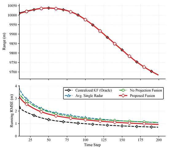
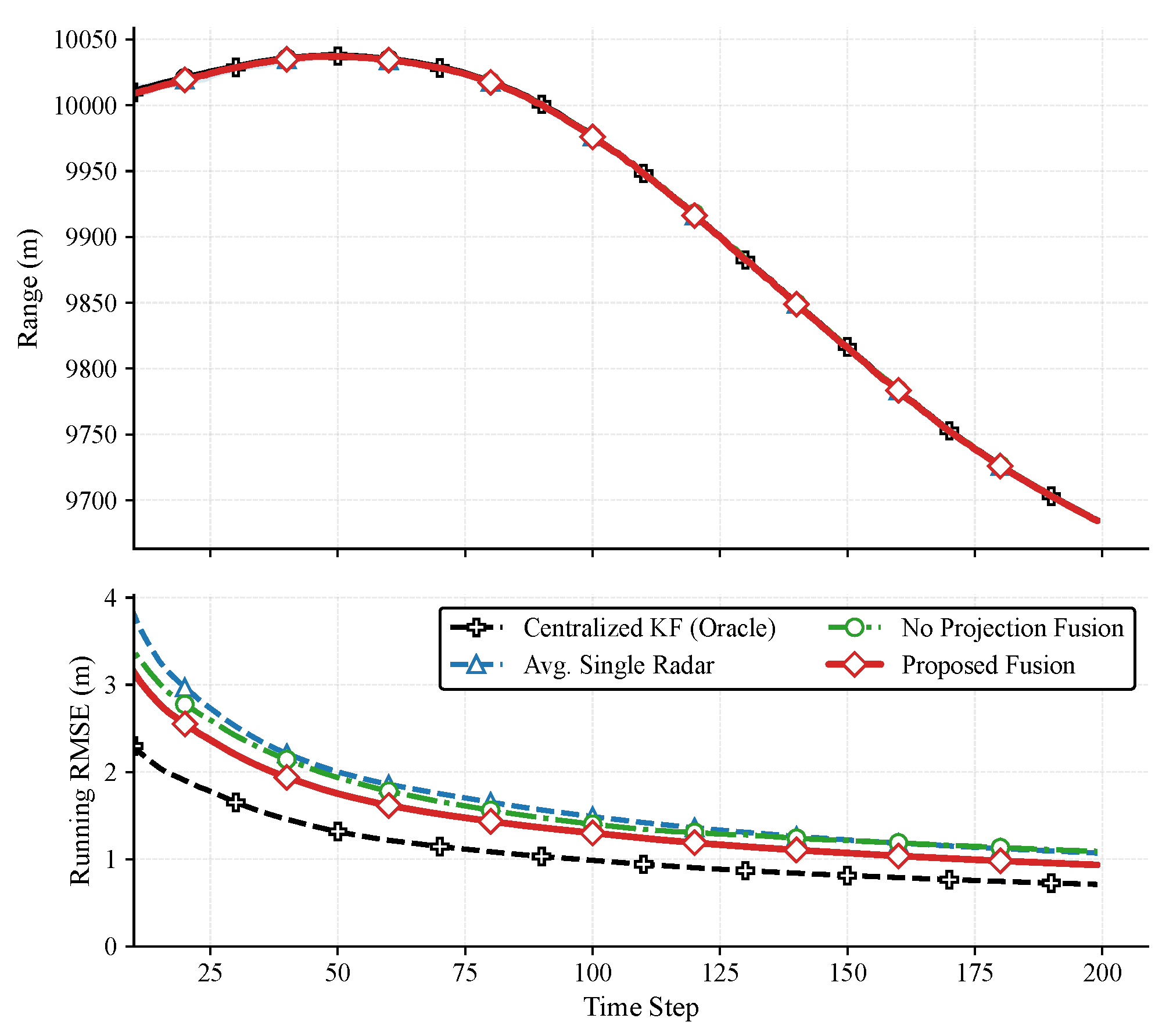
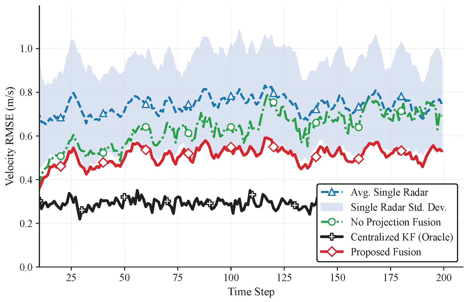
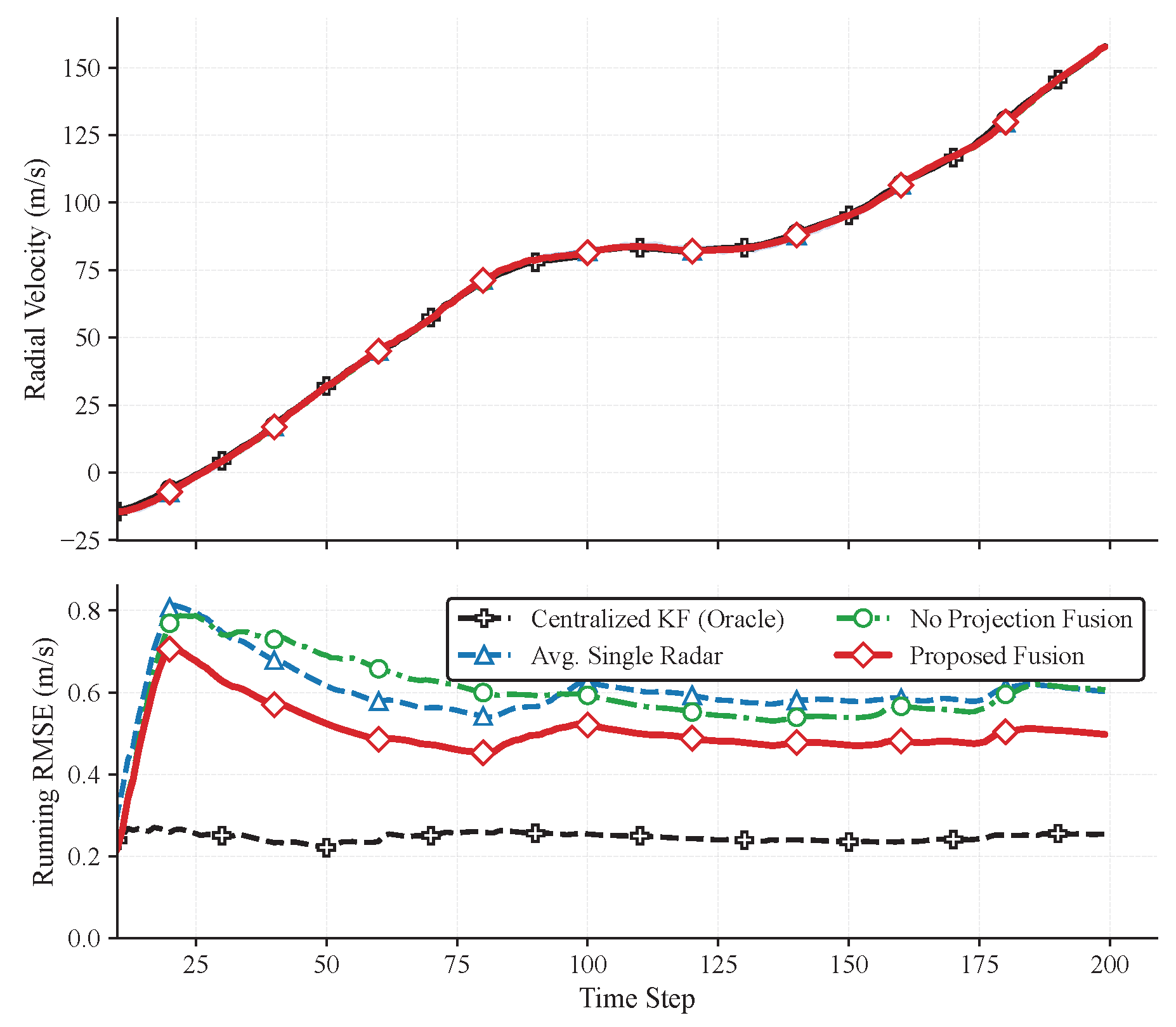
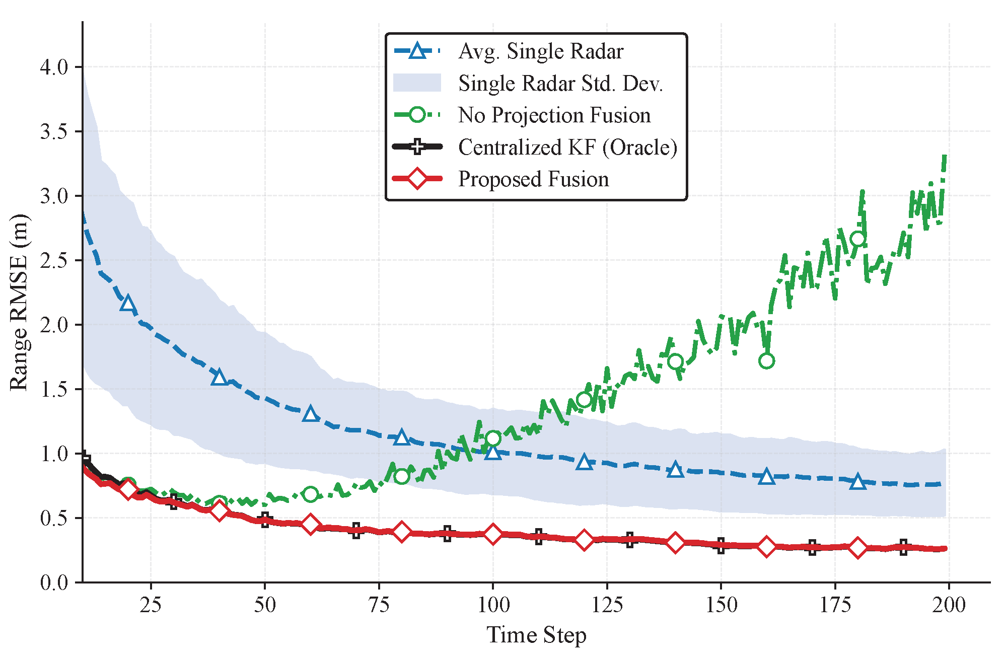
The simulation results are illustrated via tracking trajectories, RMSE evolution plots, and additional ablation/sensitivity figures. As shown in Figure 4 and Figure 5, the performance of the proposed fusion algorithm, depicted by the solid red line in all figures, is consistently superior to the individual radar estimates (represented by distinct colored lines for trajectories and by the shaded blue performance envelope in the RMSE plots).

Figure 4. Range tracking of Target 1 (top) and running RMSE (bottom, single run). Faint curves are projected single-radar tracks; the proposed track-level fusion is compared against a naive no-projection fusion baseline and a centralized measurement-level Kalman filter (Oracle).

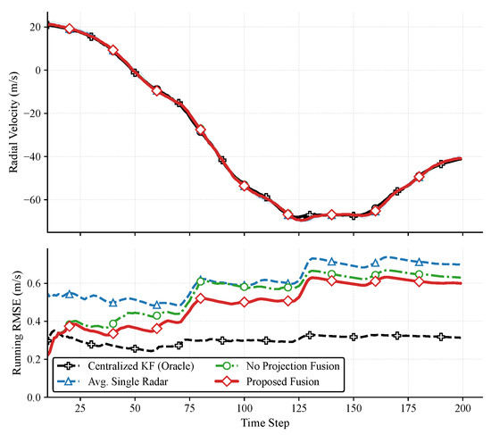
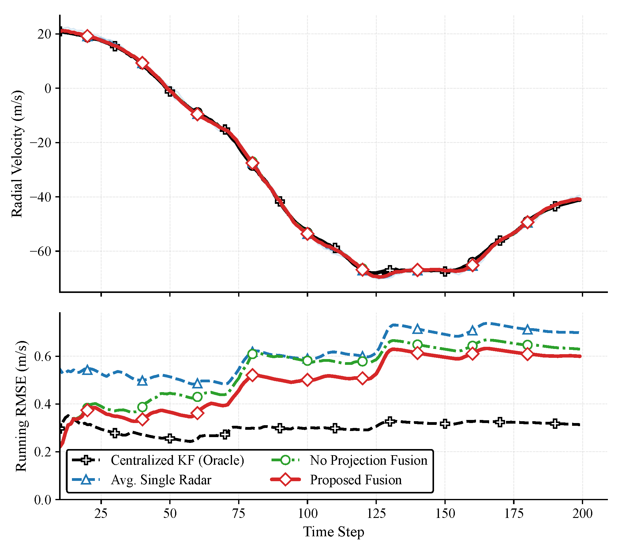
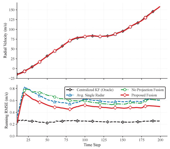
Figure 5. Velocity tracking of Target 1 (top) and running RMSE (bottom, single run). Faint curves are projected single-radar tracks; the proposed track-level fusion is compared against a naive no-projection fusion baseline and a centralized measurement-level Kalman filter (Oracle).

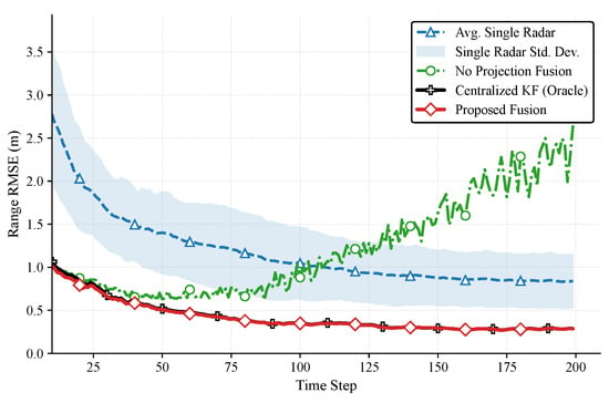
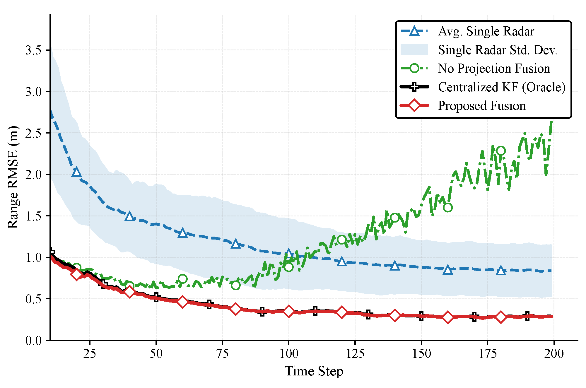
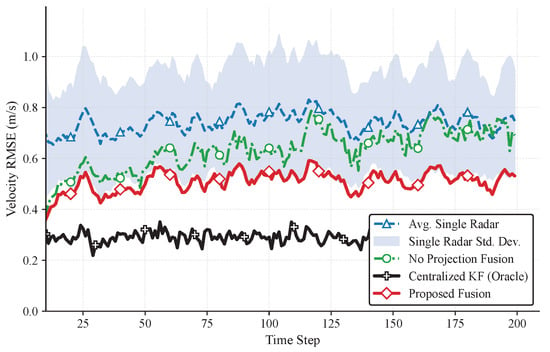
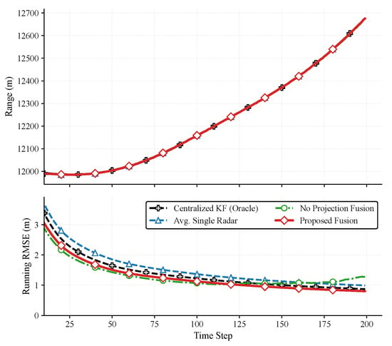
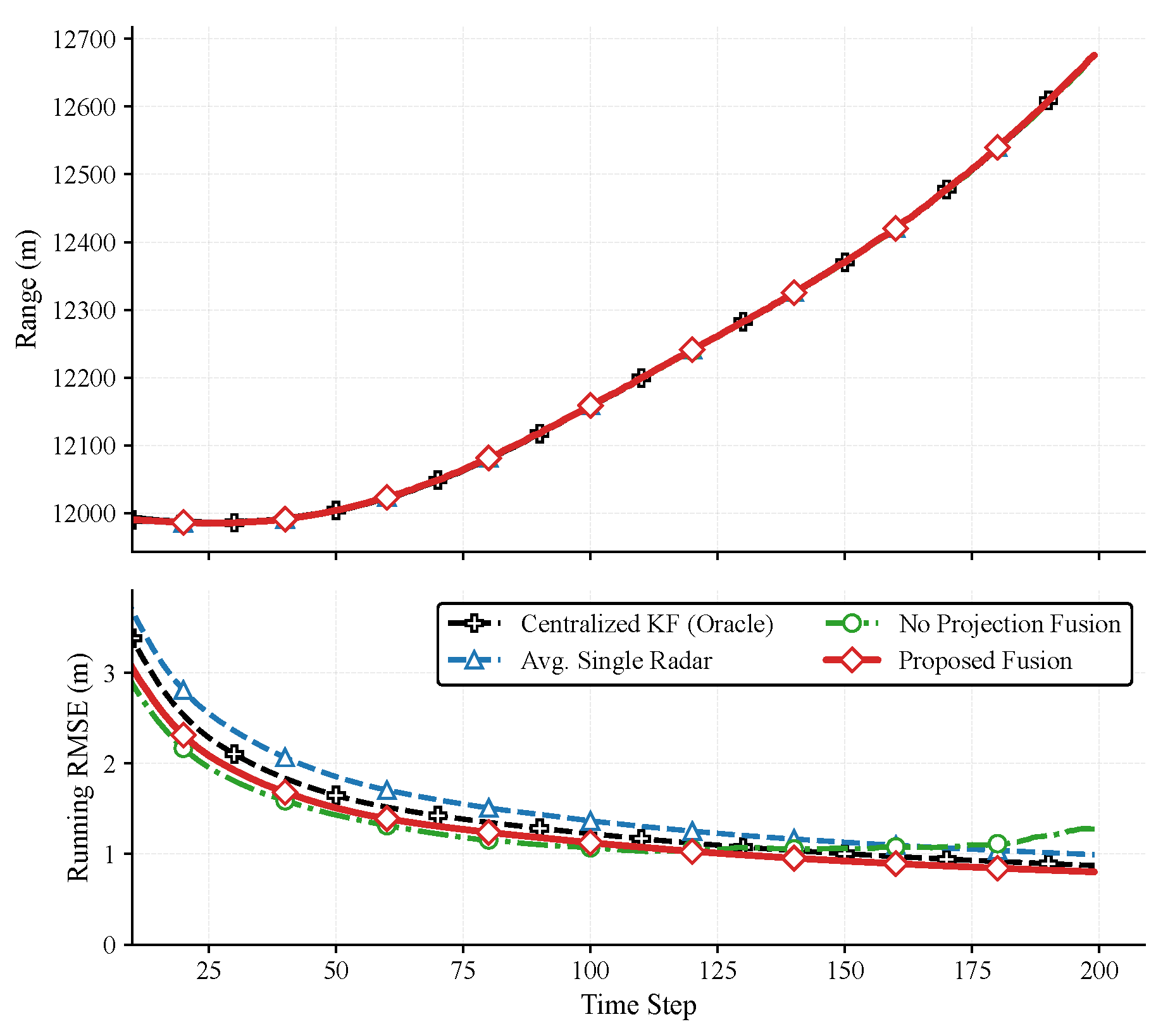
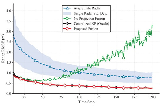
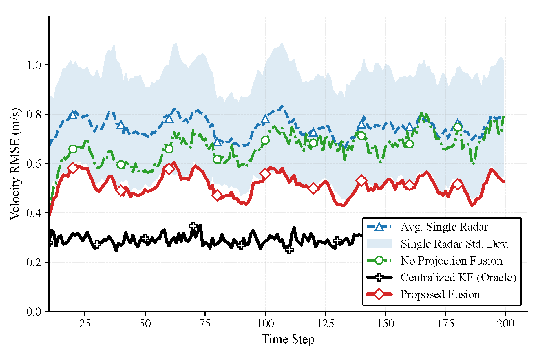
For Target 1, the steady-state fused range RMSE in Figure 6 converges to about 0.2832 m, achieving a 66.80% improvement over the average single-radar RMSE of 0.8529 m. Similarly, the radial-velocity RMSE in Figure 7 is reduced from 0.7456 m/s to 0.5204 m/s (30.21% reduction). In addition to the distributed baselines, we also report a centralized measurement-level Kalman filter (Oracle) that sequentially processes all radar measurements; it provides a performance upper bound but requires raw-measurement sharing and higher communication payload. The proposed track-level fusion approaches this oracle bound while preserving track-level communication. Importantly, under the linear-Gaussian model assumed in this paper, the Oracle baseline is equivalent to solving the centralized MAP estimation problem with all time-stamped asynchronous measurements (and thus represents MAP-based centralized optimization in this setting). As shown in Figure 8 and Figure 9, the proposed fusion achieves smoother tracking trajectories for Target 2 than the single-radar tracks and the no-projection fusion baseline. The corresponding range and radial-velocity RMSE evolutions for Target 2 are reported in Figure 10 and Figure 11.

Figure 6. Range RMSE for Target 1. The plot compares the proposed track-level fusion with the average single-radar tracker (mean ± std), a naive fusion baseline without time projection (No Projection Fusion), and a centralized measurement-level Kalman filter (Oracle).

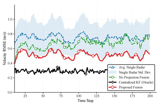
Figure 7. Velocity RMSE for Target 1. The plot compares the proposed track-level fusion with the average single-radar tracker (mean ± std), a naive fusion baseline without time projection (No Projection Fusion), and a centralized measurement-level Kalman filter (Oracle).

Figure 8. Range tracking of Target 2 (top) and running RMSE (bottom, single run). Faint curves are projected single-radar tracks; the proposed track-level fusion is compared against a naive no-projection fusion baseline and a centralized measurement-level Kalman filter (Oracle).

Figure 9. Velocity tracking of Target 2 (top) and running RMSE (bottom, single run). Faint curves are projected single-radar tracks; the proposed track-level fusion is compared against a naive no-projection fusion baseline and a centralized measurement-level Kalman filter (Oracle).

Figure 10. Range RMSE for Target 2. The plot compares the proposed track-level fusion with the average single-radar tracker (mean ± std), a naive fusion baseline without time projection (No Projection Fusion), and a centralized measurement-level Kalman filter (Oracle).

Figure 11. Velocity RMSE for Target 2. The plot compares the proposed track-level fusion with the average single-radar tracker (mean ± std), a naive fusion baseline without time projection (No Projection Fusion), and a centralized measurement-level Kalman filter (Oracle).

These gains are attributed to two key factors. First, the fusion process leverages the spatial and quality diversity of the radar network (captured in our heterogeneous ${\mathit{R}}_q$), where different radars provide complementary information. Second, the proposed time alignment via state/covariance projection ensures that all tracks are fused at a statistically consistent reference time. The inverse-covariance weighting in (26) and (27) automatically assigns more influence to estimates with smaller uncertainty, thus combining the strengths of the entire network.

More specifically, under the linear-Gaussian model with (approximately) independent projected errors, the fused mean is the MMSE-optimal solution obtained by the product of Gaussian likelihoods (Section 4). In the scalar case, if radar q provides $x_q=x+e_q$ with $e_q\sim \mathcal{N}(0,{\sigma }_q^2)$, then inverse-variance fusion yields

$${\widehat{x}}_f={\displaystyle \frac{{\sum }_q{x}_q/{\sigma }_q^2}{{\sum }_{q}1/{\sigma }_q^2}},w_q={\displaystyle \frac{1/{\sigma }_q^2}{{\sum }_{j}1/{\sigma }_j^2}},$$

which shows that a smaller uncertainty ${\sigma }_q^2$ leads to a larger weight $w_q$. In the vector case, the information matrix ${\mathit{Y}}_q={\mathit{P}}_q^{-1}$ plays the role of $1/{\sigma }_q^2$, so estimates with “smaller” covariance in the PSD sense contribute more information and thus receive higher influence through ${\mathit{P}}_q^{-1}$ in (26) and (27).

7.2.1. Angular Accuracy (Azimuth/Elevation)

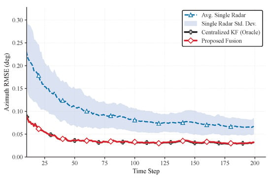
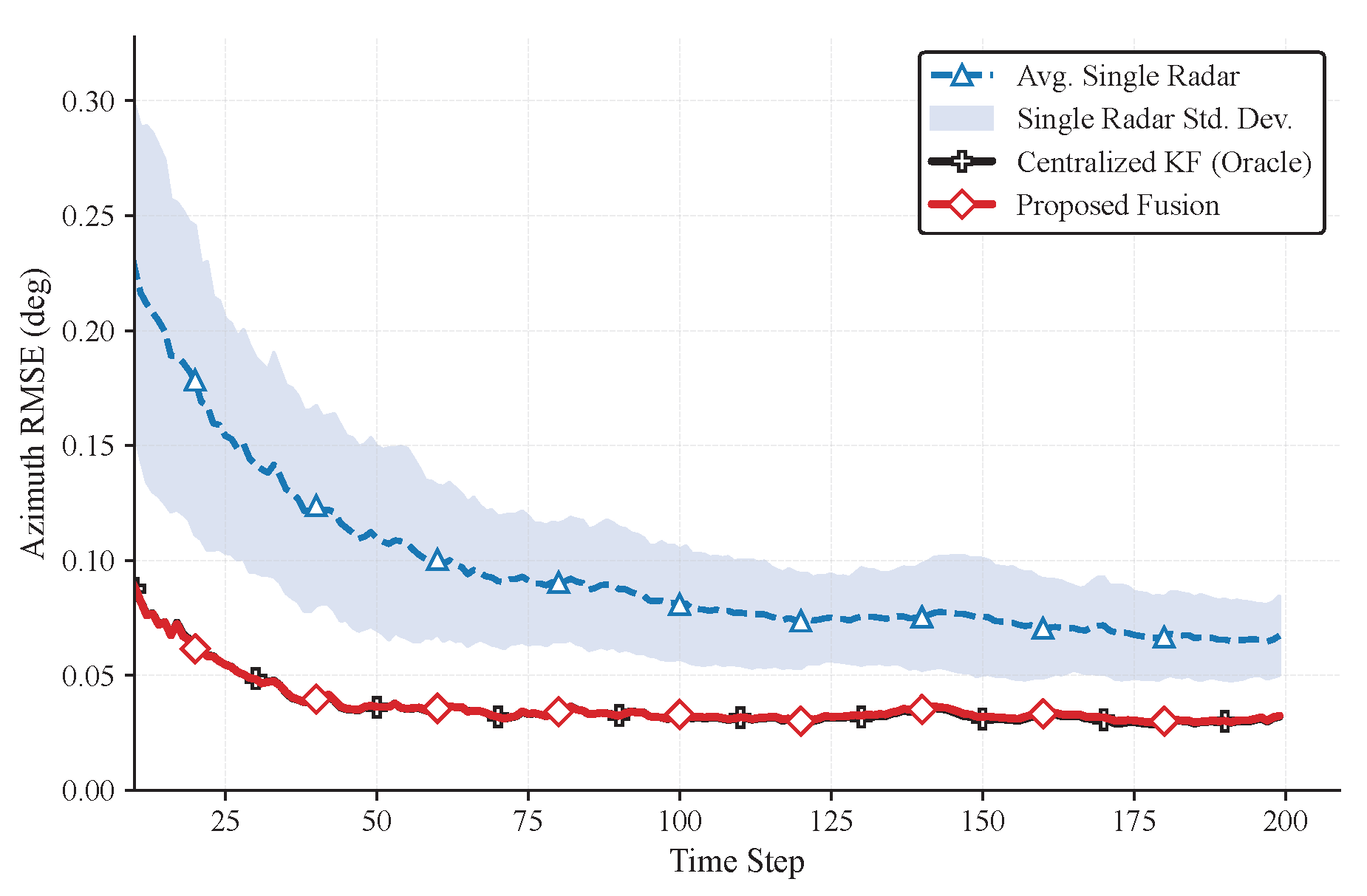
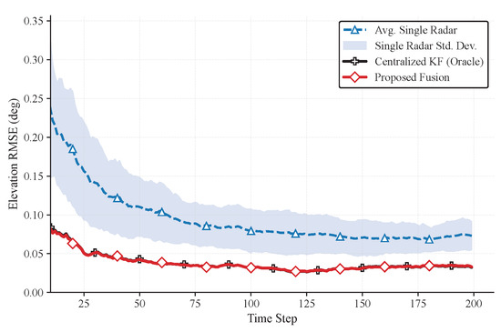
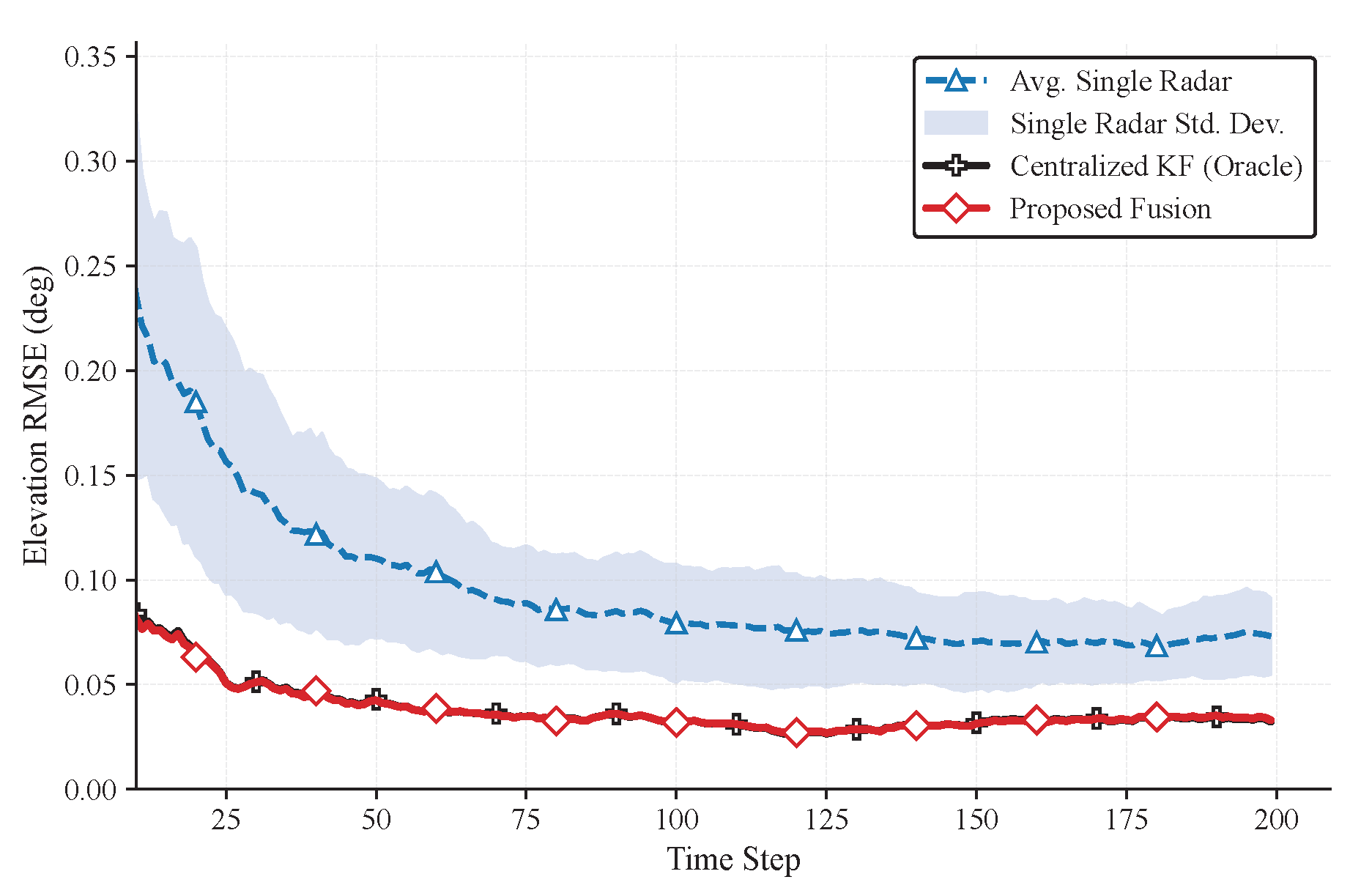
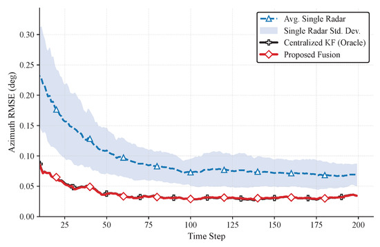
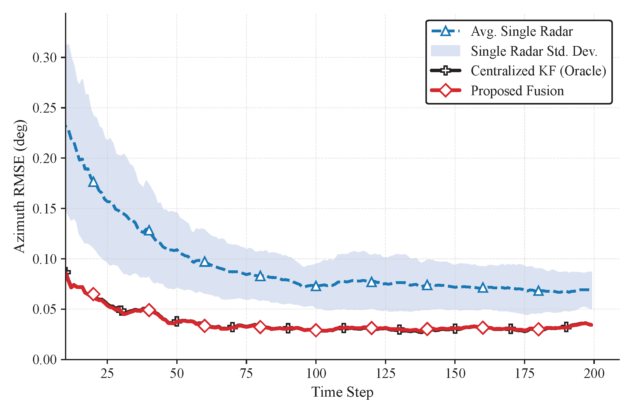
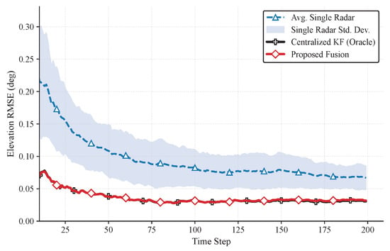
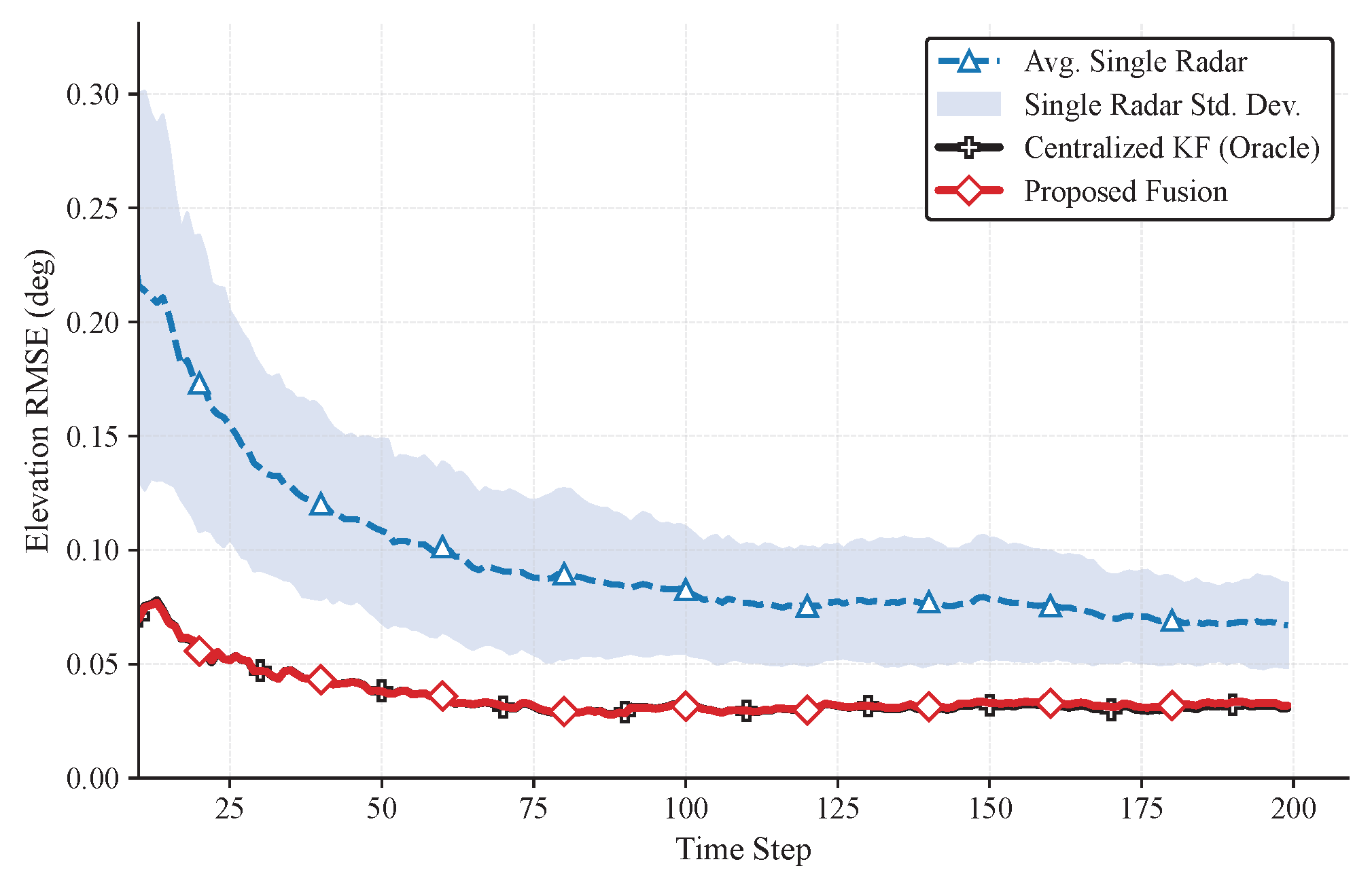
To further demonstrate that the proposed method improves the full 7D state estimate, we report the azimuth and elevation RMSE for both targets. Figure 12, Figure 13, Figure 14 and Figure 15 show consistent angular accuracy gains. The proposed fusion closely matches the centralized oracle baseline, indicating that the projection-based track fusion retains most of the benefit of measurement-level fusion despite using only track-level messages. In steady state, the proposed fusion reduces the azimuth RMSE by about 54.63% (Target 1) and 54.70% (Target 2), and reduces the elevation RMSE by about 52.62% (Target 1) and 54.52% (Target 2), relative to the average single-radar tracker.

Figure 12. Azimuth RMSE for Target 1. The plot compares the proposed track-level fusion with the average single-radar tracker (mean ± std), a naive fusion baseline without time projection (No Projection Fusion), and a centralized measurement-level Kalman filter (Oracle).

Figure 13. Elevation RMSE for Target 1. The plot compares the proposed track-level fusion with the average single-radar tracker (mean ± std), a naive fusion baseline without time projection (No Projection Fusion), and a centralized measurement-level Kalman filter (Oracle).

Figure 14. Azimuth RMSE for Target 2. The plot compares the proposed track-level fusion with the average single-radar tracker (mean ± std), a naive fusion baseline without time projection (No Projection Fusion), and a centralized measurement-level Kalman filter (Oracle).

Figure 15. Elevation RMSE for Target 2. The plot compares the proposed track-level fusion with the average single-radar tracker (mean ± std), a naive fusion baseline without time projection (No Projection Fusion), and a centralized measurement-level Kalman filter (Oracle).

7.2.2. Ablation Study

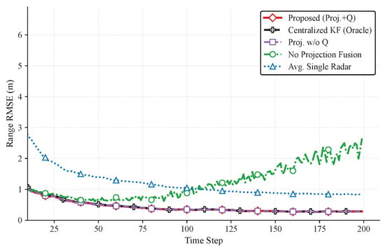
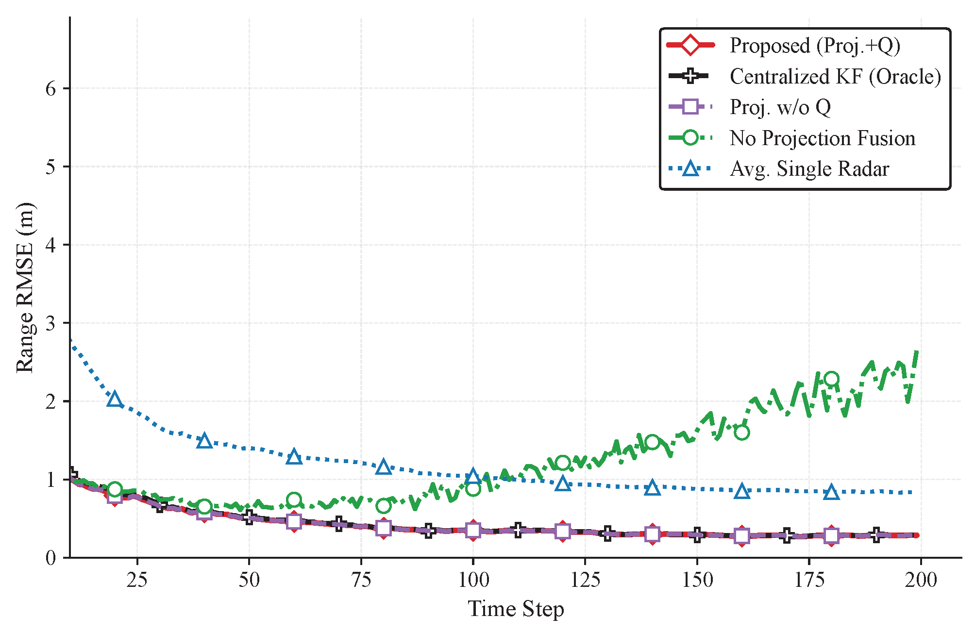
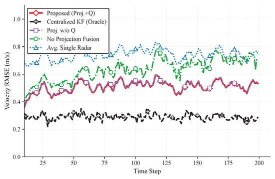
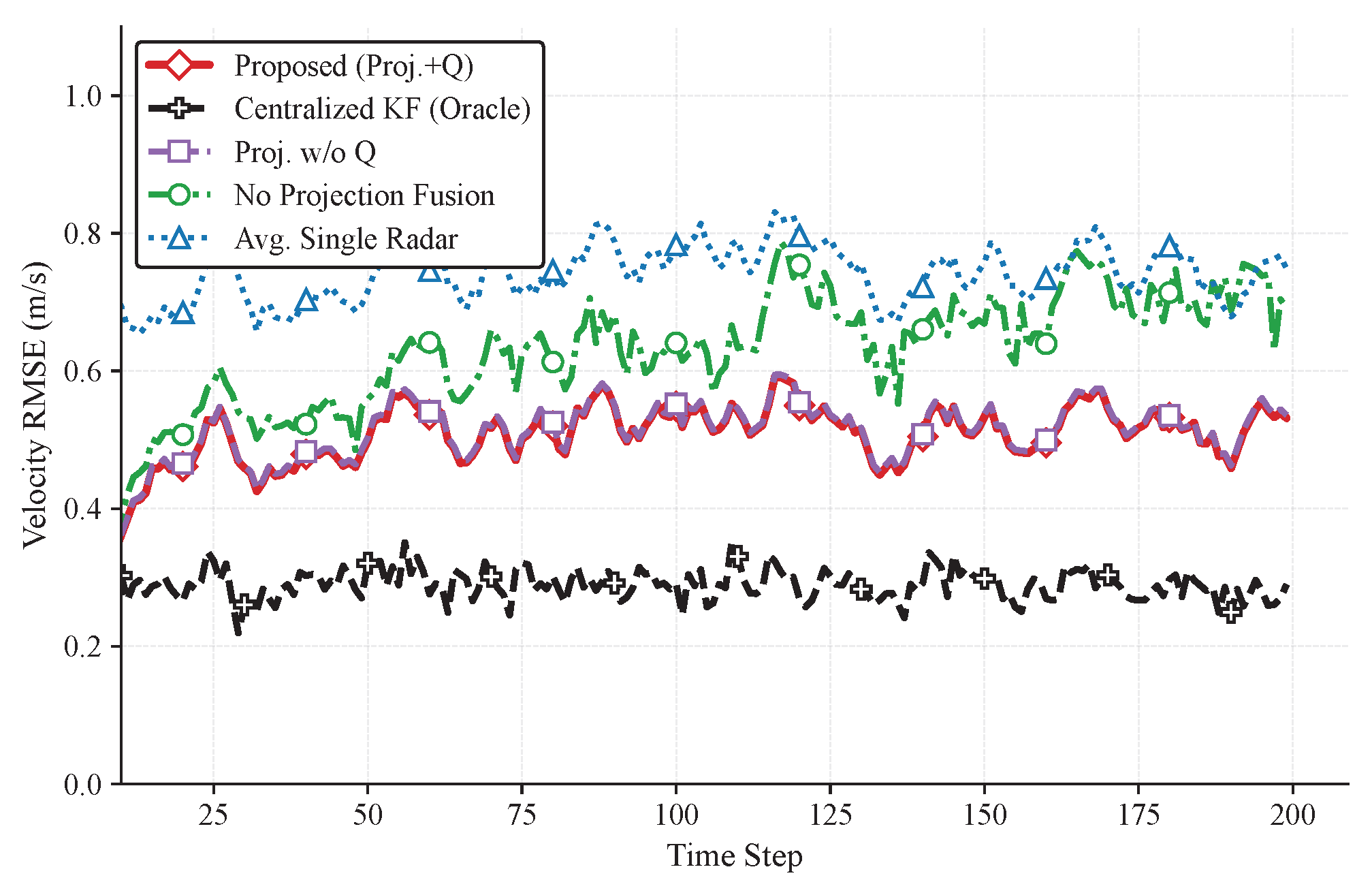
To quantify the contribution of each key design choice, we conduct an ablation study with three variants: (i) Proposed (state projection + covariance projection with $\mathit{Q}\left(\mathsf{\Delta }t\right)$); (ii) Proj. w/o $\mathit{Q}$ (covariance projection omits the $\mathit{Q}\left(\mathsf{\Delta }t\right)$ inflation term); and (iii) No Projection (direct fusion of time-misaligned local posteriors). Figure 16 and Figure 17 show that removing time projection leads to a pronounced performance loss due to temporal misalignment, especially in the range channel. While the Proj. w/o $\mathit{Q}$ variant can exhibit similar RMSE in some settings, it produces statistically overconfident covariances; this effect is captured by the consistency evaluation below.

Figure 16. Ablation on range RMSE (Target 1): proposed (Proj.+$\mathit{Q}$), Proj. w/o $\mathit{Q}$, and No Projection Fusion. Avg. single-radar and centralized Oracle are included as references.

Figure 17. Ablation on radial-velocity RMSE (Target 1): proposed (Proj.+$\mathit{Q}$), Proj. w/o $\mathit{Q}$, and No Projection Fusion. Avg. single-radar and centralized Oracle are included as references.

The No Projection baseline fuses tracks that correspond to different physical time instants. Even under a constant-velocity assumption, a time mismatch $\mathsf{\Delta }t$ induces an approximate range mismatch on the order of $v\mathsf{\Delta }t$; for accelerating motion, the mismatch includes higher-order terms. This explains why the range RMSE deteriorates more severely than the velocity RMSE when time alignment is removed. In contrast, the proposed method explicitly aligns all tracks to the same reference time via (23)–(25), converting delayed tracks into statistically consistent predictions before fusion. Moreover, the difference between Proposed and Proj. w/o $\mathit{Q}$ highlights that RMSE alone is insufficient: omitting $\mathit{Q}\left(\mathsf{\Delta }t\right)$ may not always cause a large RMSE increase at moderate offsets, but it underestimates uncertainty and can lead to overconfident fusion, as quantified by NEES below.

7.2.3. Consistency Evaluation

In addition to RMSE, we evaluate the statistical consistency of the fused estimate using the normalized estimation error squared (NEES),

$$\begin{array}{c}\hfill {\mathrm{NEES}}_{k,m}={\mathit{e}}_{k,m}^{\mathrm{T}}{\mathit{P}}_{k,m}^{-1}{\mathit{e}}_{k,m},{\mathit{e}}_{k,m}={\widehat{\mathit{x}}}_{k,m}-{\mathit{x}}_{k,m}.\end{array}$$

(43)

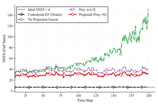
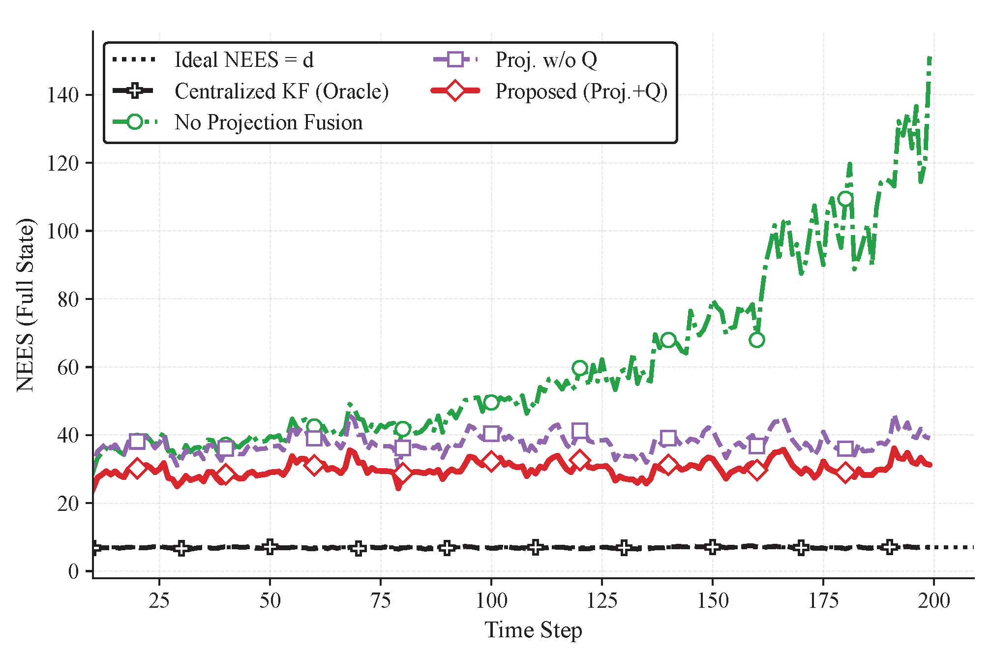
For a consistent Gaussian estimator, the expected NEES is close to the state dimension $d=7$. Figure 18 shows that the proposed method maintains NEES near d and tracks the centralized Oracle, while omitting the $\mathit{Q}\left(\mathsf{\Delta }t\right)$ inflation term leads to overconfidence (inflated NEES), confirming the necessity of covariance projection with $\mathit{Q}\left(\mathsf{\Delta }t\right)$ for consistency under temporal asynchrony.

Figure 18. Average NEES (full state) vs. time step (averaged over targets). The dotted line indicates the ideal value $d=7$.

When a local track is projected over $\mathsf{\Delta }t$, the target state evolves with independent process noise increments. If $\mathit{Q}\left(\mathsf{\Delta }t\right)$ is omitted, the projected covariance ${\mathit{P}}_{proj}$ does not account for the additional uncertainty accumulated during the projection interval, making ${\mathit{P}}_{proj}$ artificially small. Because the fusion in (26) and (27) weights each radar by ${\mathit{P}}_{proj}^{-1}$, this underestimation can overweight delayed tracks and yield an overly tight fused covariance ${\mathit{P}}_f$, which manifests as systematically inflated NEES. Therefore, the NEES result provides a critical consistency check beyond RMSE and supports the statistical necessity of covariance projection with $\mathit{Q}\left(\mathsf{\Delta }t\right)$.

7.2.4. Robustness to Highly Maneuverable Targets and Model Mismatch

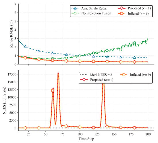
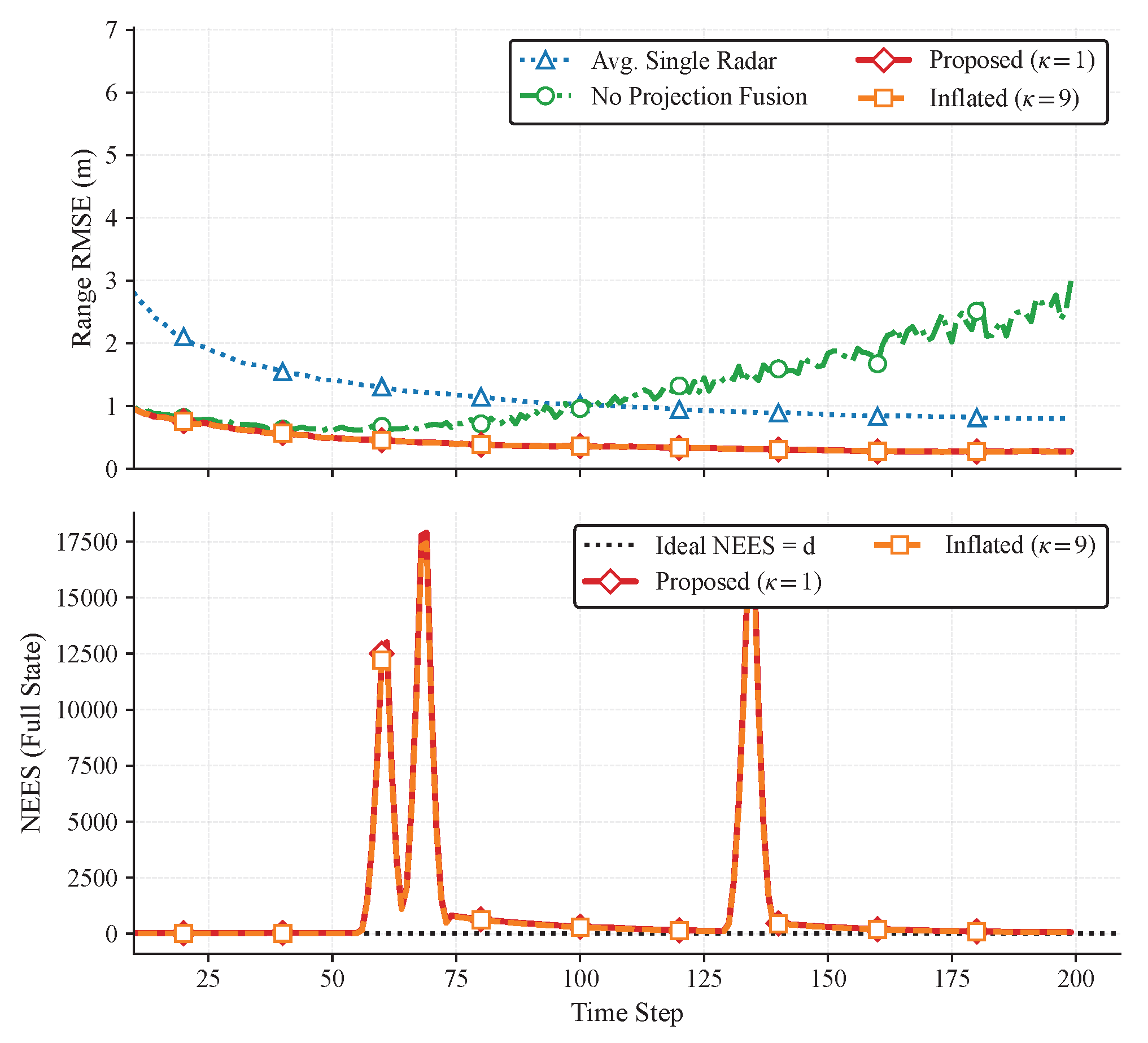
To directly address the potential model-mismatch concern under highly maneuverable targets, we further conducted a stress-test experiment where the targets execute abrupt acceleration changes and sharp turns (i.e., temporally correlated maneuver inputs) that violate the nominal CA/CV assumptions used for projection. In this setting, projection errors can be dominated by unmodeled maneuvers, and using an under-tuned $\mathit{Q}\left(\mathsf{\Delta }t\right)$ may lead to overconfident weighting of delayed tracks. We therefore evaluate the conservative inflation ${\mathit{Q}}_{\mathrm{eff}}\left(\mathsf{\Delta }t\right)$ in (9); in this stress test, we use $\kappa =9$ as a representative conservative setting. Figure 19 shows that the inflated projection uncertainty improves consistency behavior and yields a more robust accuracy–consistency trade-off under mismatch. We note that this inflation mainly improves uncertainty realism and reduces the influence of delayed tracks through inverse-covariance weighting; it does not “correct” a biased mean prediction under severe model mismatch, which motivates richer maneuver models when such complexity is feasible.

Figure 19. High-maneuver/model-mismatch stress test (averaged over targets and Monte Carlo runs). Top: range RMSE; bottom: NEES. The conservative inflation ${\mathit{Q}}_{\mathrm{eff}}\left(\mathsf{\Delta }t\right)$ (with $\kappa =9$) improves robustness by preventing severe overconfidence and by naturally down-weighting less reliable delayed tracks in information-form fusion.

7.2.5. Robustness to Unknown Cross-Correlations via Covariance Intersection

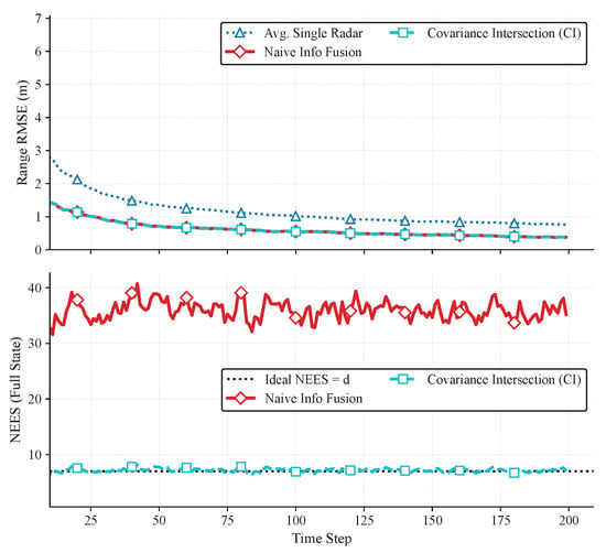
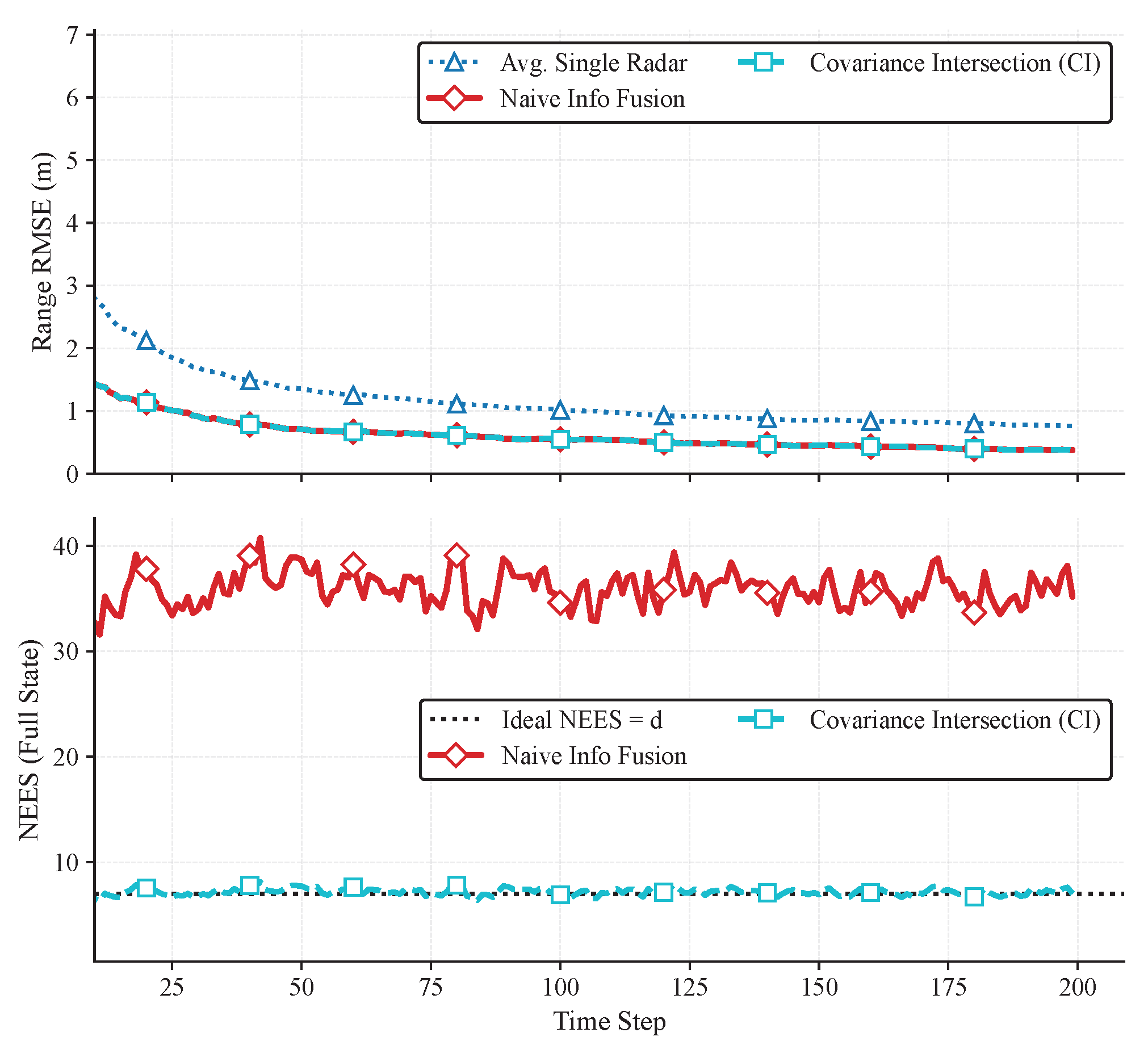
We further demonstrate the role of covariance intersection (CI) when cross-sensor correlations are unknown or unreliable. To emulate a correlated-track scenario, we add a shared measurement-noise component across radars within each fusion cycle (so that local track errors become cross-correlated, while each radar’s local filter remains consistent with its own ${\mathit{R}}_q$). In this setting, naive inverse-covariance fusion can become overconfident because it implicitly double-counts correlated information. We therefore compare naive fusion with CI (using simple equal weights ${\omega }_q=1/Q$ as a representative conservative choice). As shown in Figure 20, CI effectively mitigates overconfidence (NEES closer to the ideal value d) while yielding a comparable RMSE in this equal-weight setting; the main effect is to report a more conservative covariance under unknown cross-correlations. This clarifies its applicable scenarios and performance boundary: CI is recommended when correlations are expected (e.g., shared biases, common priors/feedback, or common unmodeled disturbances), while naive fusion remains preferable when cross-correlations are negligible and the independence assumption is approximately valid.

Figure 20. Correlated-track case (shared measurement-noise component across radars): comparison of naive information-form fusion and covariance intersection (CI). Top: range RMSE; bottom: NEES. CI reduces overconfidence under unknown cross-correlations by conservatively down-weighting the aggregated information.

7.2.6. Dynamic Network Topology: Node Addition and Exit

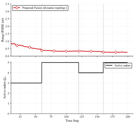
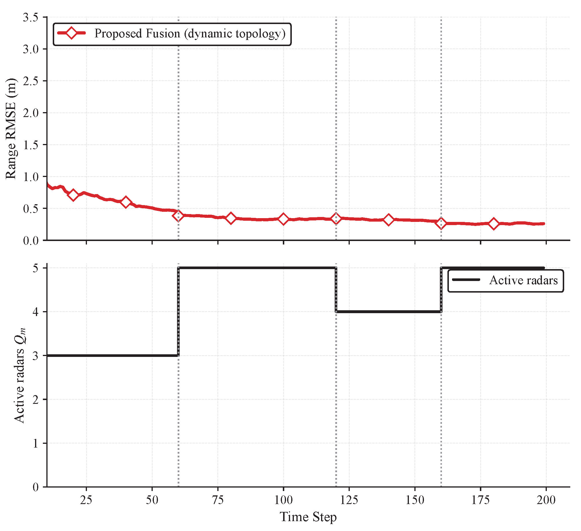
We further verify the dynamic-topology capability that naturally follows from our fusion rule, which sums information only over the available radars at each cycle. In this experiment, we emulate node addition/exit by changing the active radar set over time: two radars are absent at the beginning, then join the network, and one radar temporarily exits and later re-joins. Figure 21 shows that the proposed fusion continues to operate seamlessly and that the tracking accuracy changes smoothly as radar availability varies over time, without requiring any change to the core algorithm.

Figure 21. Dynamic network topology verification (node addition/exit). Top: range RMSE of the proposed fusion under a time-varying active radar set; bottom: the corresponding number of active radars per cycle. The fusion center naturally accommodates topology changes by summing information over available track messages.

7.2.7. Sensitivity to Time Asynchrony

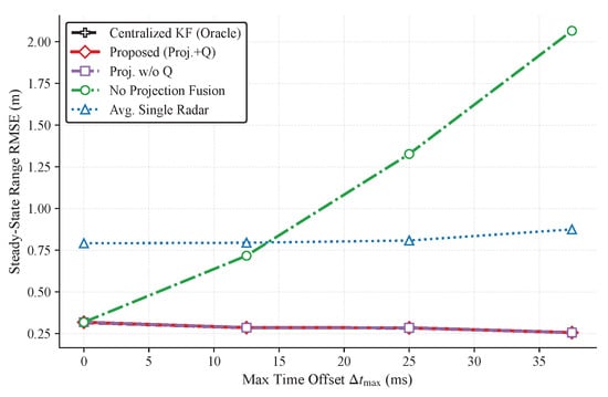
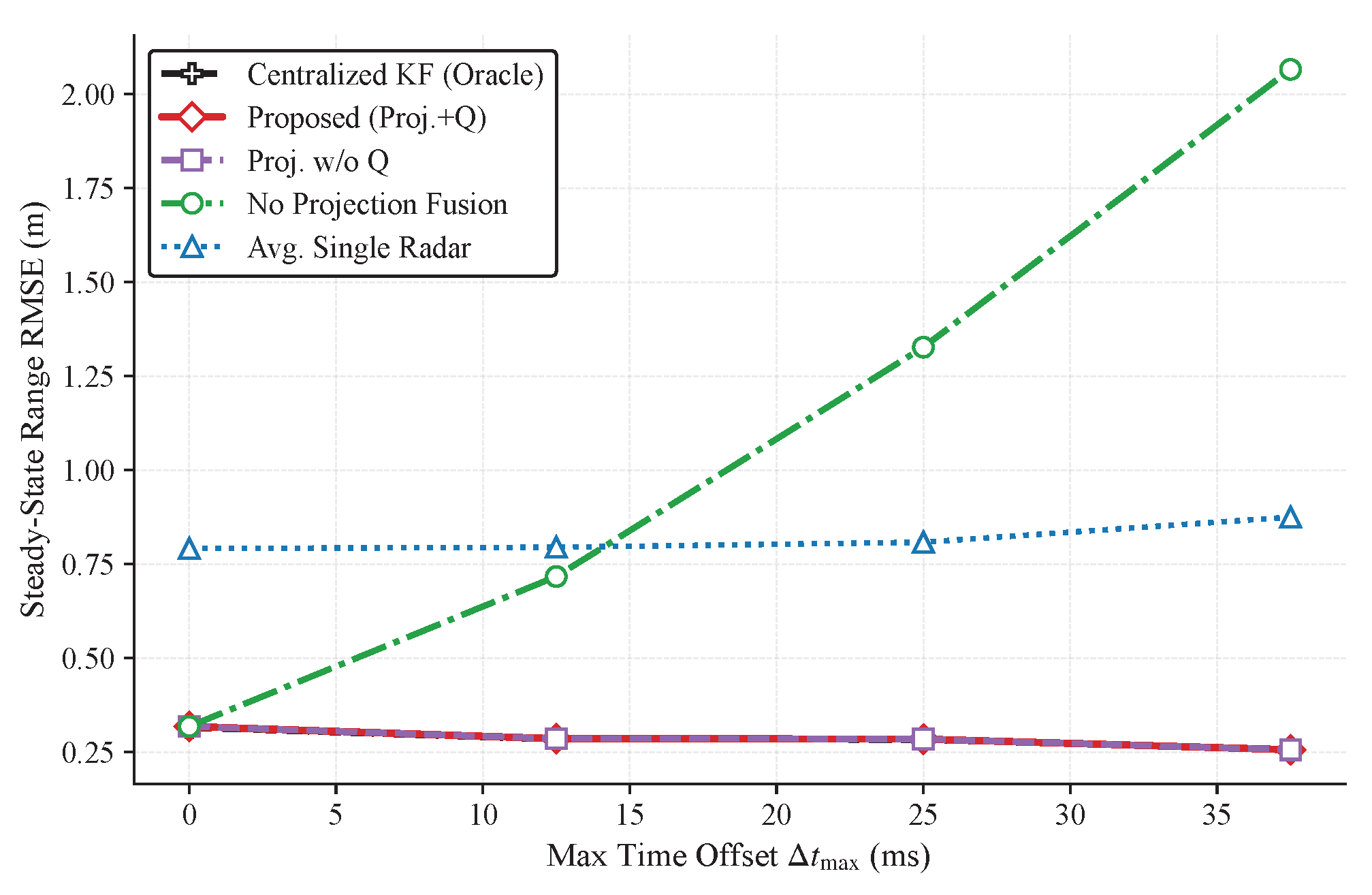
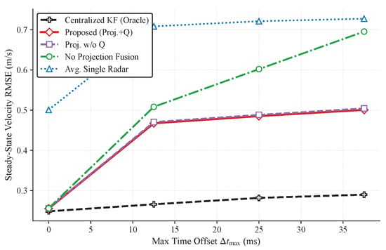
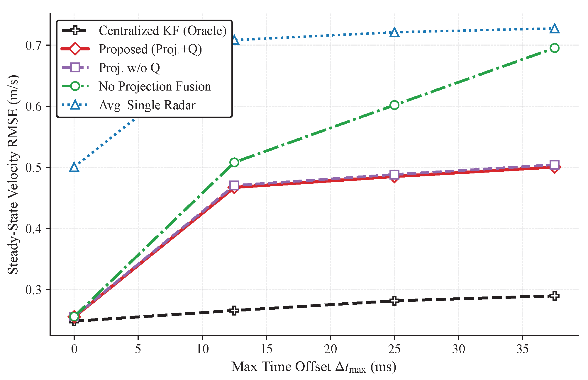
We sweep the maximum time offset $\mathsf{\Delta }{t}_{max}$ from 0 to $0.75T_p$ and report the steady-state RMSE averaged over targets. Figure 22 and Figure 23 indicate that the proposed method degrades gracefully with increasing asynchrony and consistently outperforms the track-level baselines, while remaining close to the centralized Oracle bound.

Figure 22. Steady-state range RMSE vs. maximum time offset $\mathsf{\Delta }{t}_{max}$, comparing the proposed method and baselines (averaged over targets).

Figure 23. Steady-state radial-velocity RMSE vs. maximum time offset $\mathsf{\Delta }{t}_{max}$, comparing the proposed method and baselines (averaged over targets).

Increasing $\mathsf{\Delta }{t}_{max}$ enlarges the projection intervals, which increases the projected uncertainty through $\mathit{Q}\left(\mathsf{\Delta }t\right)$ and reduces the effective information contributed by delayed tracks (Section 5.2). The proposed method degrades gracefully because this delay-induced uncertainty is explicitly modeled and thus stale tracks are automatically down-weighted during fusion. In contrast, No Projection suffers from both deterministic time mismatch (tracks correspond to different times) and improper weighting, and thus exhibits much faster degradation, especially in the range channel.

7.2.8. Scaling with the Number of Radars

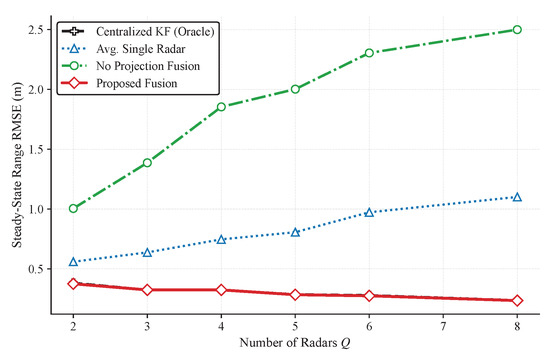
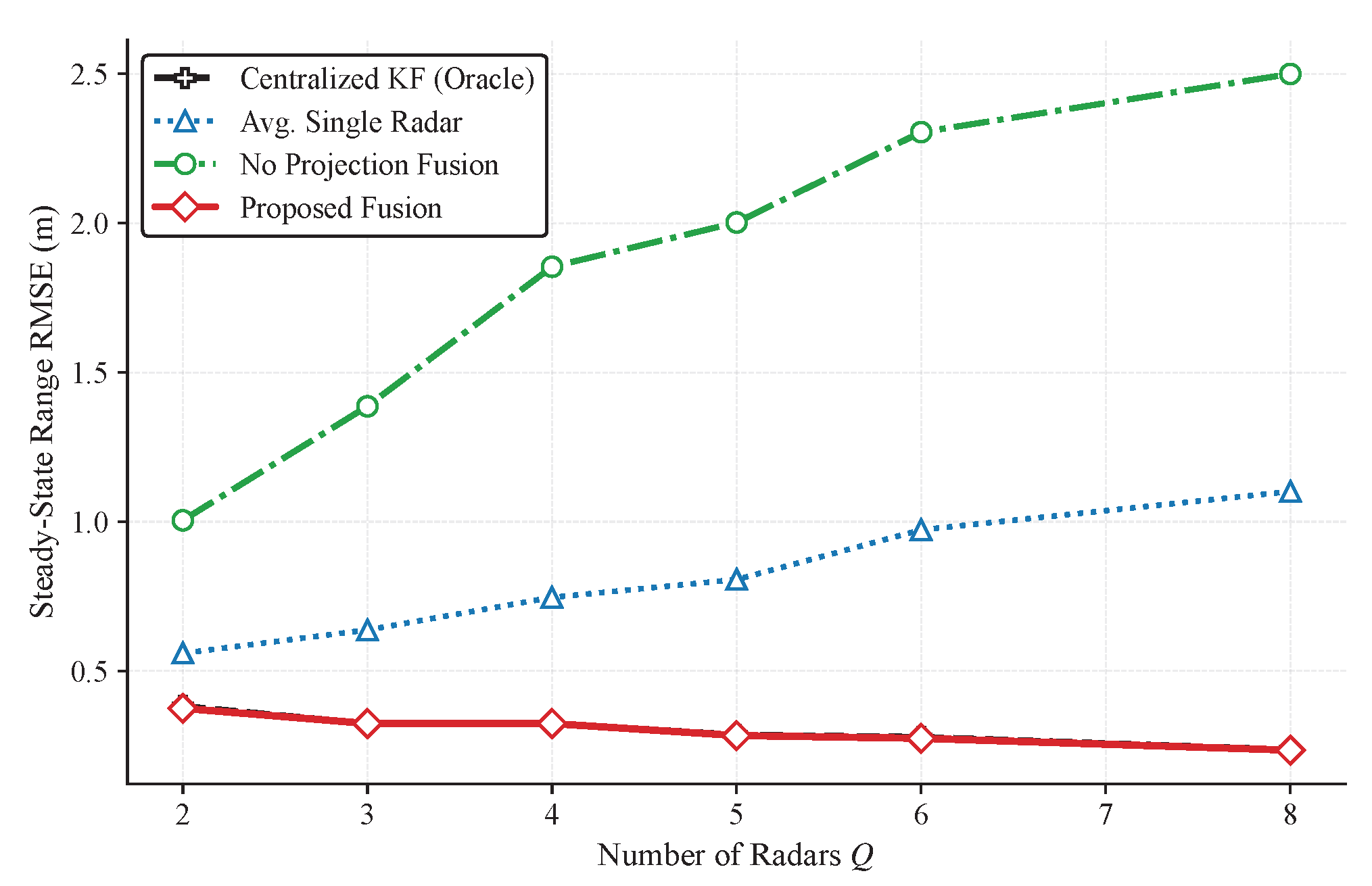
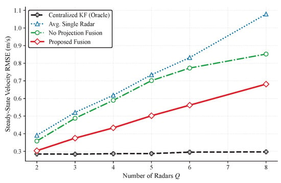
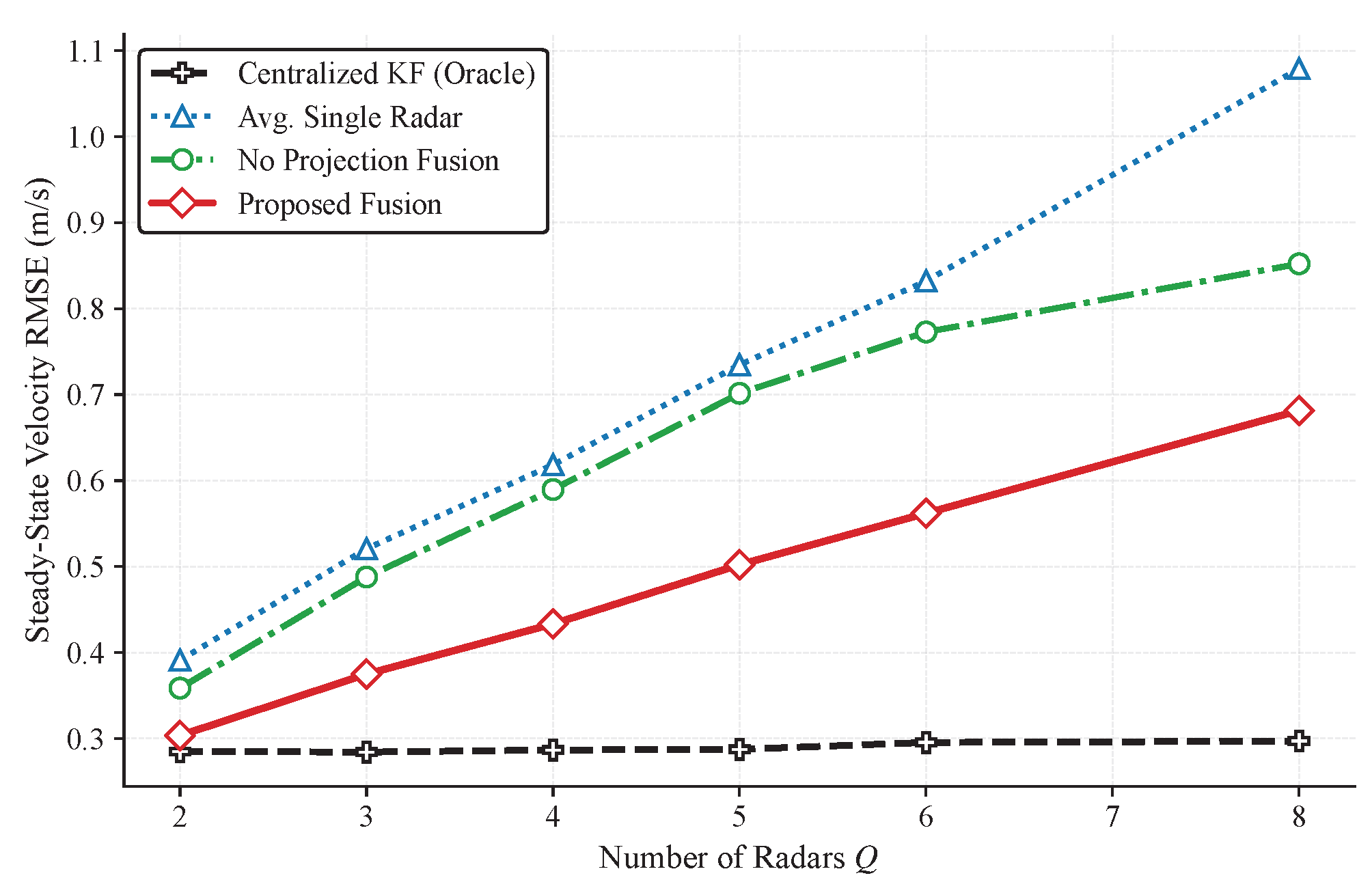
Finally, we vary the number of radars Q and evaluate the steady-state RMSE of the proposed method together with representative baselines. Figure 24 and Figure 25 show that the proposed method consistently outperforms the track-level baselines and that the accuracy improves as more radars participate in fusion, with diminishing returns as Q becomes large. The centralized Oracle curve provides an upper bound and highlights the performance–communication trade-off.

Figure 24. Steady-state range RMSE vs. number of radars Q, comparing the proposed method and baselines (averaged over targets).

Figure 25. Steady-state radial-velocity RMSE vs. number of radars Q, comparing the proposed method and baselines (averaged over targets).

Under the approximate independence assumption, information matrices add (Section 5.3): ${\mathit{P}}_f^{-1}={\sum }_q{\mathit{P}}_q^{-1}$. If sensors have comparable quality, this suggests that uncertainty decreases roughly proportionally to Q and RMSE decreases approximately as $1/\sqrt{Q}$, while diminishing returns arise when a few high-quality radars dominate the information sum or when projection noise reduces the effective information of more delayed tracks. Importantly, the communication payload also scales linearly with Q (one compact track message per radar), making the Q-sweep results a direct illustration of the accuracy–communication trade-off enabled by track-level fusion. For the 7D Gaussian track message used in this paper, adding one radar increases the per-update payload by $35K$ scalars (Table 3); thus, Figure 24 and Figure 25 can also be read as accuracy vs. communication-payload scaling.

Second, the algorithm demonstrates strong robustness to temporal asynchrony. This directly follows from the state and covariance projection steps in (23) and (25), where each local estimate is propagated to a common reference time and its uncertainty is inflated by $\mathit{Q}\left(\mathsf{\Delta }{t}_{q,m}\right)$ to reflect the accumulated process noise over the projection interval. As a result, older (more delayed) information is automatically down-weighted during fusion, maintaining statistical consistency. This behavior is further supported by the ablation results (Figure 16 and Figure 17) and the time-offset sweeps (Figure 22 and Figure 23), where the proposed method degrades gracefully with increasing $\mathsf{\Delta }{t}_{max}$ and consistently outperforms non-projected or noise-omitting variants.

The performance gains are consistent across different target dynamics, as shown by the results for Target 2 (Figure 8, Figure 9, Figure 10 and Figure 11). Despite following a decelerating trajectory, Target 2 achieves comparable steady-state accuracy improvements: the fused range RMSE decreases from 0.7981 m to 0.2728 m (65.82% reduction), and the fused radial-velocity RMSE decreases from 0.7476 m/s to 0.5117 m/s (31.55% reduction). Averaged over the two targets, the proposed fusion provides about 66.31% range RMSE reduction and 30.88% radial-velocity RMSE reduction relative to the average single-radar tracker.

In addition to range and radial velocity, the proposed fusion also improves angular estimation. Averaged over the two targets, the steady-state azimuth RMSE is reduced from about 0.0693° to 0.0314° (about 55% reduction), and the steady-state elevation RMSE is reduced from about 0.0711° to 0.0331° (about 54% reduction), confirming that the proposed method consistently enhances the full state estimate.

These results, combined with the analysis in Section 6, highlight the core achievement of this work: the proposed method achieves substantial tracking gains under asynchronous operation while retaining a communication-efficient track-level information exchange. The computational complexity of $O\left(KQ{d}^3\right)$ remains manageable for real-time systems, making the algorithm a practical solution for communication-constrained multi-radar networks.

7.2.9. Comprehensive Discussion of Experimental Findings

The experiments provide several practically relevant observations. The proposed track-level fusion consistently approaches the centralized measurement-level oracle while exchanging only compact track messages, indicating that under the adopted linear-Gaussian setting, a large portion of the useful information can be preserved in the track domain. The ablation results also verify that explicit time alignment is essential in asynchronous fusion, because directly combining time-misaligned posteriors can degrade performance, especially for the range channel.

Beyond accuracy curves, the NEES evaluation provides an application-oriented consistency check that is particularly important in radar networking. In practical multi-target systems, the reported covariance directly affects gating probabilities, data association decisions, track confirmation/termination logic, and even sensor scheduling and resource management. Overconfident covariances can shrink gates and increase missed associations and track fragmentation, while overly conservative covariances can enlarge gates and raise false associations and computational burden. The sensitivity and scaling studies further show that the proposed method degrades gracefully with increasing asynchrony and benefits from additional radars with diminishing returns, which is consistent with the additive information interpretation in Section 5.

8. Discussion

8.1. Limitations

The proposed framework has several limitations that motivate future work. The MMSE optimality of inverse-covariance fusion relies on (approximate) independence across radars after projection. In practical systems, cross-correlations may arise due to shared priors, common modeling assumptions, or feedback, which can make naive fusion overconfident. When cross-covariances are unknown, conservative alternatives such as covariance intersection (CI) (Section 4, Robust Fusion under Unknown Cross-Correlations) can be adopted. To address this point, we added an explicit correlated-track simulation in Section 7 (Figure 20) to illustrate when naive fusion becomes overconfident and how CI provides a conservative and more consistent alternative under unknown cross-correlations.

The current formulation also adopts a linear state-space model with Gaussian noises and a hybrid CA/CV motion model for projection. While this choice is effective for moderate maneuvers when process-noise levels are tuned appropriately, highly maneuvering targets with abrupt acceleration changes, coordinated snake-like motions, or strong nonlinearities can induce model mismatch and degrade projection accuracy, especially over larger time offsets. Extending the framework to model sets and nonlinear/non-Gaussian filtering, such as IMM, EKF/UKF, or particle-filter-based fusion, is a natural direction to improve generality under complex dynamics and disturbances. We further clarify the trade-off between (i) keeping a simple CA/CV projection with conservative uncertainty inflation and (ii) adopting richer maneuver models to reduce mismatch. The inflation factor $\kappa$ mainly guards against overconfident weighting by expanding the projected covariance, but it cannot guarantee that the projected mean remains accurate when the motion model induces a biased projection error (Section 5.1, Remark on model mismatch). In contrast, coordinated-turn/Singer/IMM-type models can reduce mismatch but increase local filtering complexity and fusion-center projection complexity. To keep the communicated message as “state + covariance”, an IMM tracker can be moment-matched to a single Gaussian at each timestamp; transmitting multiple model-conditioned components/probabilities provides higher fidelity but increases payload and requires mixture-aware projection/fusion at the center. Such heterogeneous-model extensions also introduce additional system-engineering and synchronization requirements (e.g., consistent time bases/state definitions and explicit model/meta-data), and mismatches across nodes may cause inconsistent projection and potential numerical/estimation instability if not handled carefully. We therefore avoid claiming a cost-free “plug-and-play” upgrade and instead describe these as modular extensions with explicit engineering trade-offs.

Finally, although our simulations focus on sensing timestamp offsets, practical deployments may face additional uncertainties in time stamping, calibration, and networking. Timestamps are assumed to be comparable at the fusion center (e.g., after coarse synchronization or offset compensation), and residual time-varying clock errors can translate into uncertainty in $\mathsf{\Delta }t$ and thus into additional projection uncertainty. Moreover, packet loss, out-of-order arrivals, and transmission delays beyond timestamp misalignment are not explicitly modeled and may require out-of-sequence update mechanisms or robust asynchronous scheduling. The projection noise $\mathit{Q}\left(\mathsf{\Delta }t\right)$ further depends on process-noise parameters, and the fusion assumes that local tracks are expressed in a compatible state space; mis-tuning or calibration errors can affect weighting and overall performance.

8.2. Practical Deployment Considerations and Extensions

Several practical aspects are worth discussing for real-world deployment. Since each track message carries an explicit timestamp, the fusion center can decouple sensing time from message arrival time and operate in an event-driven manner by fusing whichever subset of tracks is available at a given fusion instant and projecting tracks to a chosen reference time; missing tracks simply do not contribute to the information sum. In practice, time-varying clock offsets can be handled when timestamps are expressed in, or mapped to, a common time base at the fusion center, and residual clock errors can be treated as additional uncertainty in $\mathsf{\Delta }t$ by conservatively inflating the projection uncertainty when necessary. Communication latency and variable transmission delay primarily manifest as delayed availability of track messages; for late or out-of-sequence arrivals, buffering with a short fixed-lag window, applying out-of-sequence update (OOSM) techniques, re-fusing within a sliding window, or discarding overly stale tracks are reasonable compensation strategies, while a detailed design depends on the network stack and latency budget.

The information-form fusion also naturally supports dynamic network topology, because the fusion rule sums over the set of available radars at each cycle. In practice, topology changes mainly affect track management (e.g., association/initialization) and the consistency of coordinate frames, which can be handled by standard track management modules and sensor calibration/registration. For real-time or embedded implementation with $d=7$, the dominant operations in fusion are small matrix multiplications and linear solves; efficient implementations can exploit the block-diagonal CA/CV structure, use Cholesky factorization/solve instead of explicit matrix inversion, and precompute closed-form $\mathit{F}\left(\mathsf{\Delta }t\right)$ and $\mathit{Q}\left(\mathsf{\Delta }t\right)$. When the number of targets or update rates become large, additional engineering optimizations such as parallelization across targets/radars and hardware acceleration for small-matrix operations can further reduce latency and computational resource usage.

Beyond Gaussian assumptions, one possible direction is to run particle filtering (or Gaussian-mixture filtering) locally and transmit either moment-matched Gaussian track messages (mean/covariance) or low-order mixture summaries, followed by approximate fusion at the center, while another direction is to use variational inference to maintain a tractable Gaussian (or structured) approximation when incorporating nonlinear/non-Gaussian likelihood factors. Finally, when time asynchrony becomes extremely large relative to the sampling interval or the target maneuver time scale, projected uncertainties inflate via $\mathit{Q}\left(\mathsf{\Delta }t\right)$ and the effective contribution of delayed tracks diminishes; in this regime, the fused estimate tends to rely primarily on the most recent and highest-quality tracks, and the achievable gain over the best single-radar tracker naturally shrinks.

9. Conclusions

This paper has proposed a communication efficient asynchronous track level fusion framework for multi-radar systems. The proposed framework has selected a causal reference time at the fusion center and has projected local state and covariance estimates to this common time while accounting for the uncertainty accumulated during the projection interval. This design has enabled statistically sound information-form fusion for asynchronously arriving tracks. To reduce communication overhead, each radar has performed local Kalman filtering and has transmitted only a compact track message containing the estimated state, its uncertainty, and a timestamp, rather than raw measurements. For the adopted state dimension, the symmetric covariance has been communicated using only a few dozen scalar values per target per update, which has made the approach suitable for bandwidth constrained networks. The computational cost per fusion cycle has scaled linearly with the number of targets and radars for a fixed state dimension, and has been dominated by small matrix operations, which has supported real-time implementation with standard embedded optimizations. Monte Carlo simulations with heterogeneous radars and time asynchrony on the order of tens of milliseconds have demonstrated substantial accuracy and robustness gains. Compared with an average single-radar tracker, the fused solution has reduced steady-state range error by roughly two thirds and radial-velocity error by about one third, and has also improved angular accuracy by about one half. The consistency evaluation has further confirmed that properly inflating the projected uncertainty has been necessary to avoid overconfident covariance reporting in asynchronous fusion.

In practical deployments, cross-sensor correlations mainly arise from shared information paths such as common initialization priors, shared biases/disturbances, or feedback of fused tracks to local trackers. When the architecture allows explicit bookkeeping of such common information, the fusion center can maintain or approximate cross-covariances by propagating the shared prior through the known local filter models and timestamps, enabling exact correlated-track fusion. Otherwise, correlations can be assessed empirically via innovation-based consistency monitoring (e.g., normalized innovation squared (NIS) statistics) and handled conservatively by adopting covariance intersection (CI) or other bounding/inflation strategies. Importantly, this is a modular choice in our pipeline: after time alignment via state/covariance projection, we use information-form fusion under approximate independence, switch to CI when cross-covariances are unknown/unreliable, and can plug in exact correlated fusion when cross-covariances are available. Future work will extend the framework to strongly correlated tracks, highly maneuvering targets, and nonlinear or non-Gaussian environments, and will incorporate realistic communication effects such as packet loss and out-of-sequence arrivals. Validation on real multi-radar data has also been identified as an important next step for practical deployment.

References

- Yuan, Y.; Liu, X.; Li, W.; Yi, W.; Choi, W. Decentralized Resource Allocation for Multi-Radar Systems Based on Quality of Service Framework. IEEE Trans. Signal Process. 2024, 72, 1189–1204. [Google Scholar] [CrossRef] [Scilit]
- Ren, M.; He, P.; Zhou, J. Improved Shape-Based Distance Method for Correlation Analysis of Multi-Radar Data Fusion in Self-Driving Vehicle. IEEE Sens. J. 2021, 21, 24771–24781. [Google Scholar] [CrossRef] [Scilit]
- Choi, W.Y.; Lee, S.H.; Chung, C.C. On-Road Object Collision Point Estimation by Radar Sensor Data Fusion. IEEE Trans. Intell. Transp. Syst. 2022, 23, 14753–14763. [Google Scholar] [CrossRef] [Scilit]
- Tang, Z.; Pan, X.; She, X.; Zhao, J. NIR-RGB-M2Net: A Fusion Model for Precise Agricultural Field Segmentation Using Multisource Remote Sensing Data. IEEE J. Sel. Top. Appl. Earth Obs. Remote Sens. 2025, 18, 19988–20004. [Google Scholar] [CrossRef] [Scilit]
- Liu, Q.; Guo, R.; Wang, J.; Xu, S.; Chen, Z. Signal-Level Fusion-Based Height Estimation of Low-Elevation Target for Distributed Radar. IEEE Trans. Instrum. Meas. 2025, 74, 1–14. [Google Scholar] [CrossRef] [Scilit]
- Jamal, S.; Sun, G.; Li, Y.; Khan, A.Q.; Zhang, Y.; Verlanti, A.; Nunziata, F. CWCM-Net: A Novel Feature Fusion Method for Oil Spill Detection Using Single- and Quad-Polarization SAR Data. IEEE J. Sel. Top. Appl. Earth Obs. Remote Sens. 2025, 18, 19115–19128. [Google Scholar] [CrossRef] [Scilit]
- Chen, P.; Zhou, T.; Chen, Z.; Meng, F.; Liu, J. BFP-Net: A DL-based ISAC beamforming prediction method for extended vehicle. Veh. Commun. 2025, 55, 100945. [Google Scholar] [CrossRef] [Scilit]
- Li, A.; Zheng, B.; Li, L. Intelligent Transportation Application and Analysis for Multi-Sensor Information Fusion of Internet of Things. IEEE Sens. J. 2021, 21, 25035–25042. [Google Scholar] [CrossRef] [Scilit]
- Yang, Y.; Gui, S.; Zhao, Q.; Wan, Q. Deep-Unfolded Fusion Optimization With Motion Correlation Learning for ViSAR Multi-GMTIm. IEEE Trans. Instrum. Meas. 2025, 74, 1–18. [Google Scholar] [CrossRef] [Scilit]
- Zhao, S.; Zhang, L.; Zhou, Y.; Liu, N. Signal Fusion-Based Algorithms to Discriminate Between Radar Targets and Deception Jamming in Distributed Multiple-Radar Architectures. IEEE Sens. J. 2015, 15, 6697–6706. [Google Scholar] [CrossRef] [Scilit]
- Zhang, K.; Wang, Z.; Guo, L.; Peng, Y.; Zheng, Z. An Asynchronous Data Fusion Algorithm for Target Detection Based on Multi-Sensor Networks. IEEE Access 2020, 8, 59511–59523. [Google Scholar] [CrossRef] [Scilit]
- Hestrio, Y.F.; Surya Candra, D.; Prima Brahmantara, R.; Prabowo, Y.; Dimara Sakti, A.; Luthfi Ramadhan, M.M.; Loong Yap, Y.; Azizah, K.; Hafizhuddin Hilman, M.; Phinn, S.; et al. Fusion+: A Multi-Sensor Image Fusion for Very High-Resolution Satellite Imagery. IEEE Access 2025, 13, 62856–62869. [Google Scholar] [CrossRef] [Scilit]
- Lu, P.; Dai, F. An Overview of Multi-sensor Information Fusion. In Proceedings of the 2021 6th International Conference on Intelligent Informatics and Biomedical Sciences (ICIIBMS), Oita, Japan, 25–27 November 2021; Volume 6, pp. 5–9. [Google Scholar] [CrossRef] [Scilit]
- Lindenmaier, L.; Czibere, B.; Aradi, S.; Bécsi, T. A Robust and Runtime-Efficient Track-to-Track Fusion for Automotive Perception Systems. IEEE Sens. J. 2025, 25, 14022–14035. [Google Scholar] [CrossRef] [Scilit]
- Li, H.; Mehul, A.; Le Kernec, J.; Gurbuz, S.Z.; Fioranelli, F. Sequential Human Gait Classification With Distributed Radar Sensor Fusion. IEEE Sens. J. 2021, 21, 7590–7603. [Google Scholar] [CrossRef] [Scilit]
- Luan, T.; Zhang, H.; Li, J.; Zhang, J.; Zhuo, L. Object Fusion Tracking for RGB-T Images via Channel Swapping and Modal Mutual Attention. IEEE Sens. J. 2023, 23, 22930–22943. [Google Scholar] [CrossRef] [Scilit]
- Sanson, J.B.; Castanheira, D.; Gameiro, A.; Monteiro, P.P. Cooperative Method for Distributed Target Tracking for OFDM Radar With Fusion of Radar and Communication Information. IEEE Sens. J. 2021, 21, 15584–15597. [Google Scholar] [CrossRef] [Scilit]
- Aeberhard, M.; Schlichtharle, S.; Kaempchen, N.; Bertram, T. Track-to-Track Fusion With Asynchronous Sensors Using Information Matrix Fusion for Surround Environment Perception. IEEE Trans. Intell. Transp. Syst. 2012, 13, 1717–1726. [Google Scholar] [CrossRef] [Scilit]
- Wang, S.; Mei, L.; Liu, R.; Jiang, W.; Yin, Z.; Deng, X.; He, T. Multi-Modal Fusion Sensing: A Comprehensive Review of Millimeter-Wave Radar and Its Integration With Other Modalities. IEEE Commun. Surv. Tutor. 2025, 27, 322–352. [Google Scholar] [CrossRef] [Scilit]
- Lim, T.Y.; Markowitz, S.A.; Do, M.N. RaDICaL: A Synchronized FMCW Radar, Depth, IMU and RGB Camera Data Dataset With Low-Level FMCW Radar Signals. IEEE J. Sel. Top. Signal Process. 2021, 15, 941–953. [Google Scholar] [CrossRef] [Scilit]
- Liu, R.W.; Guo, Y.; Nie, J.; Hu, Q.; Xiong, Z.; Yu, H.; Guizani, M. Intelligent Edge-Enabled Efficient Multi-Source Data Fusion for Autonomous Surface Vehicles in Maritime Internet of Things. IEEE Trans. Green Commun. Netw. 2022, 6, 1574–1587. [Google Scholar] [CrossRef] [Scilit]
- Chen, Y.; Sheng, X.; Guo, L.; Li, P.; Hao, H.; Yin, J. Asynchronous Multisonar Data Integration Approach Used to Detect Sparse Targets. IEEE Access 2019, 7, 37908–37917. [Google Scholar] [CrossRef] [Scilit]
- Zhou, Y.; Zhang, L.; Cao, Y.; Huang, Y. Optical-and-Radar Image Fusion for Dynamic Estimation of Spin Satellites. IEEE Trans. Image Process. 2020, 29, 2963–2976. [Google Scholar] [CrossRef] [PubMed]
Disclaimer/Publisher’s Note: The statements, opinions and data contained in all publications are solely those of the individual author(s) and contributor(s) and not of MDPI and/or the editor(s). MDPI and/or the editor(s) disclaim responsibility for any injury to people or property resulting from any ideas, methods, instructions or products referred to in the content. |
© 2026 by the authors. Licensee MDPI, Basel, Switzerland. This article is an open access article distributed under the terms and conditions of the Creative Commons Attribution (CC BY) license.