Edge Exemplars Enhanced Incremental Learning Model for Tor-Obfuscated Traffic Identification

Abstract

Tor is the most widely used anonymous communication network. Tor has developed a series of pluggable transports (PTs) to obfuscate traffic and avoid censorship. These PTs use different traffic obfuscation techniques, and many of them have been maintained and updated. In order to achieve continual learning against PTs and their updates, this paper proposes an incremental learning model for Tor traffic detection. First, we analyzed several common traffic obfuscation techniques, including randomization, mimicry, and tunneling. A feature set was designed for Tor obfuscation traffic detection. Second, this paper constructs the Tor incremental learning framework and proposes edge exemplar enhancement to enhance the memory of trained models for previous classes. It can enhance the previous class memory of the model through edge feature enhancement and selective replay to alleviate the catastrophic forgetting problem of incremental learning. Finally, we combined public and self-collected datasets to simulate the development of Tor PTs and verify the effectiveness of our model. The experimental results show that the improved model in this paper has the highest accuracy rate of 87.6% in the simulated environment. This means that the incremental learning model can effectively cope with the updating of PTs.

1. Introduction

With the rapid development of network information technology, internet users are increasingly concerned about their personal privacy. Although many encryption protocols have been developed to protect the privacy of communications, such as HTTPS, SSH, etc., the real identity of users cannot be hidden by employing these protocols, and their IP or other private information may be intercepted. In order to further protect the privacy of communications, many anonymous communication networks have been developed, such as Tor [1], I2P [2], Freenet [3], etc. Among them, Tor has become the most widely used anonymous communication network due to its simple deployment and high performance. Tor is a network composed of virtual channels that send communication traffic through three random servers in the Tor network: the entry node, the relay node, and the exit node. Notably, its nodes are provided by volunteers from various countries. In addition to providing anonymous communication services, Tor also provides hidden services, also known as the dark web. Many examples of illegal content are hosted on the dark web. These users utilized Tor to cover these illegal activities. Therefore, the detection and monitoring of Tor traffic are significant ways to ensure network security.

Many organizations and internet service providers have a low tolerance for anonymous traffic. They design detection systems to detect Tor traffic and block anonymous communications over Tor for various reasons. As a result, Tor traffic detection technology and Tor censorship circumvention technology are constantly escalating the process of confrontation. In the early days, Tor traffic was directly encrypted using TLS. But there are several fixed patterns in the packets during the connection process. This allows the censor to directly use deep packet inspection (DPI) methods to detect Tor traffic. To further protect the availability of Tor, pluggable transports (PTs) are designed to bypass network censorship. Pluggable transports are a mechanism for quickly developing and deploying anti-censorship tools, using modular subsystems to transform traffic. It will start a proxy process on the client and obfuscate the traffic through proxy nodes (known as bridges) before it reaches the server host. Tor has had many different built-in PTs throughout its history. The latest version of Tor includes obfs4, Meek-azure, and Snowflake as three different bridges.

The extensive use of PTs increases the difficulty of detecting Tor traffic. Whether it is the encryption and randomization obfuscation technology of Obfs4 or the domain fronting technology of Meek, they all blur the traffic characteristics of Tor anonymous communication. Meanwhile, these traffic obfuscation techniques make it difficult for traffic inspectors to identify Tor traffic by DPI. However, we consider that the biggest challenge in detecting anonymous Tor communication traffic to lie in the confrontation between detection and obfuscation. The PTs provide a platform for Tor traffic obfuscation, on which various traffic obfuscation techniques are rapidly developed and iterated. From the perspective of historical versions, it has already been experienced from Obfs2 to Obfs4, from Flashproxy to Snowflake. While these obfuscation techniques are iteratively updated, their detection methods also need to be updated. This requires the detection model to have the capability of continuous learning. Therefore, we propose a Tor traffic obfuscation detection framework based on incremental learning in this paper. Under this framework, the traffic types for model detection are extensible. When new PT traffic is discovered, there is no need to retrain the model using all of the training data. In the face of PT updates and upgrades, this method can effectively save data storage space and model training time. The main contributions of this paper are as follows:

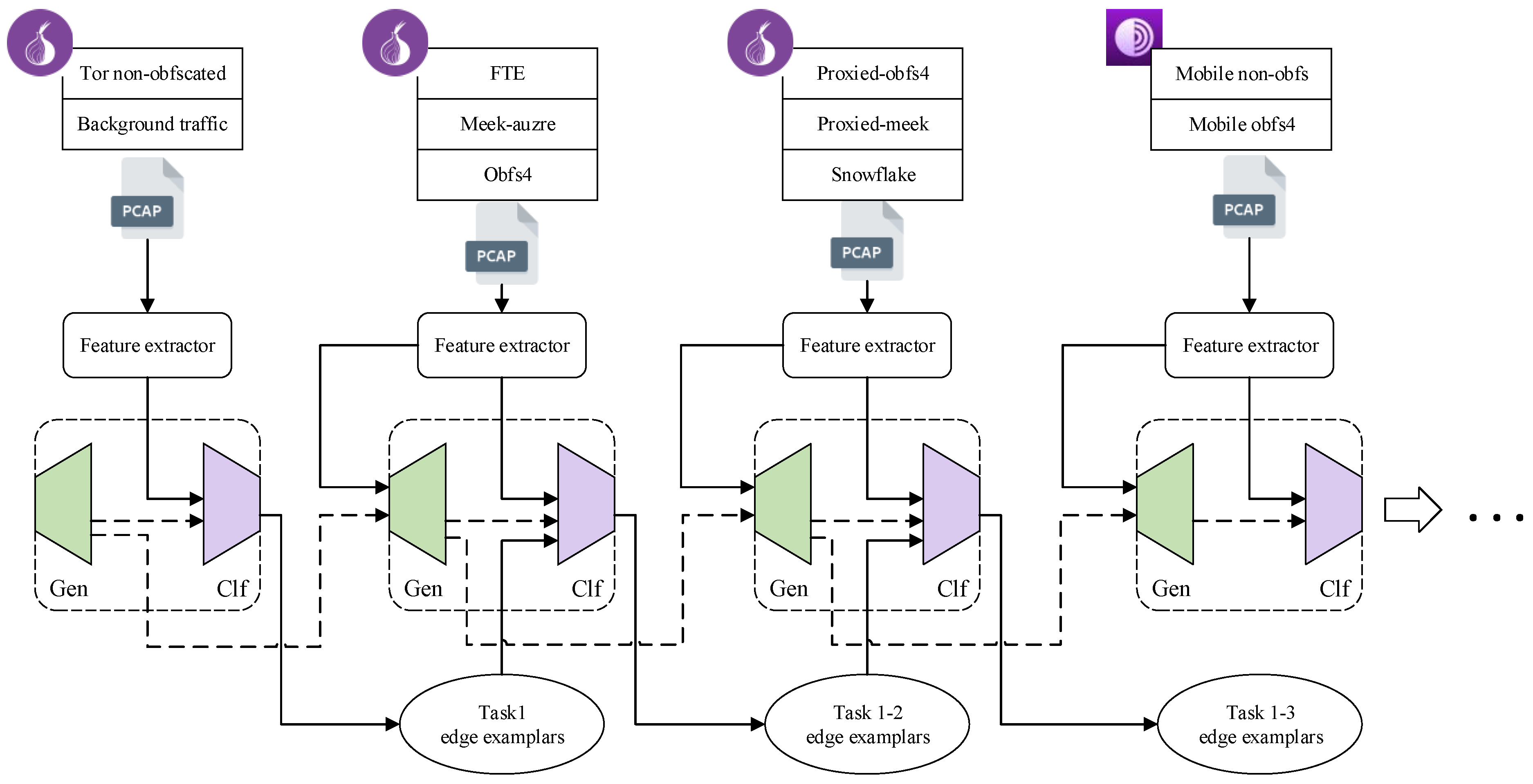
• An incremental learning framework is designed for Tor-obfuscated traffic detection. Adding new types of obfuscated traffic requires only incremental updates to existing models. Compared with retraining, it effectively saves data storage space and model training time.
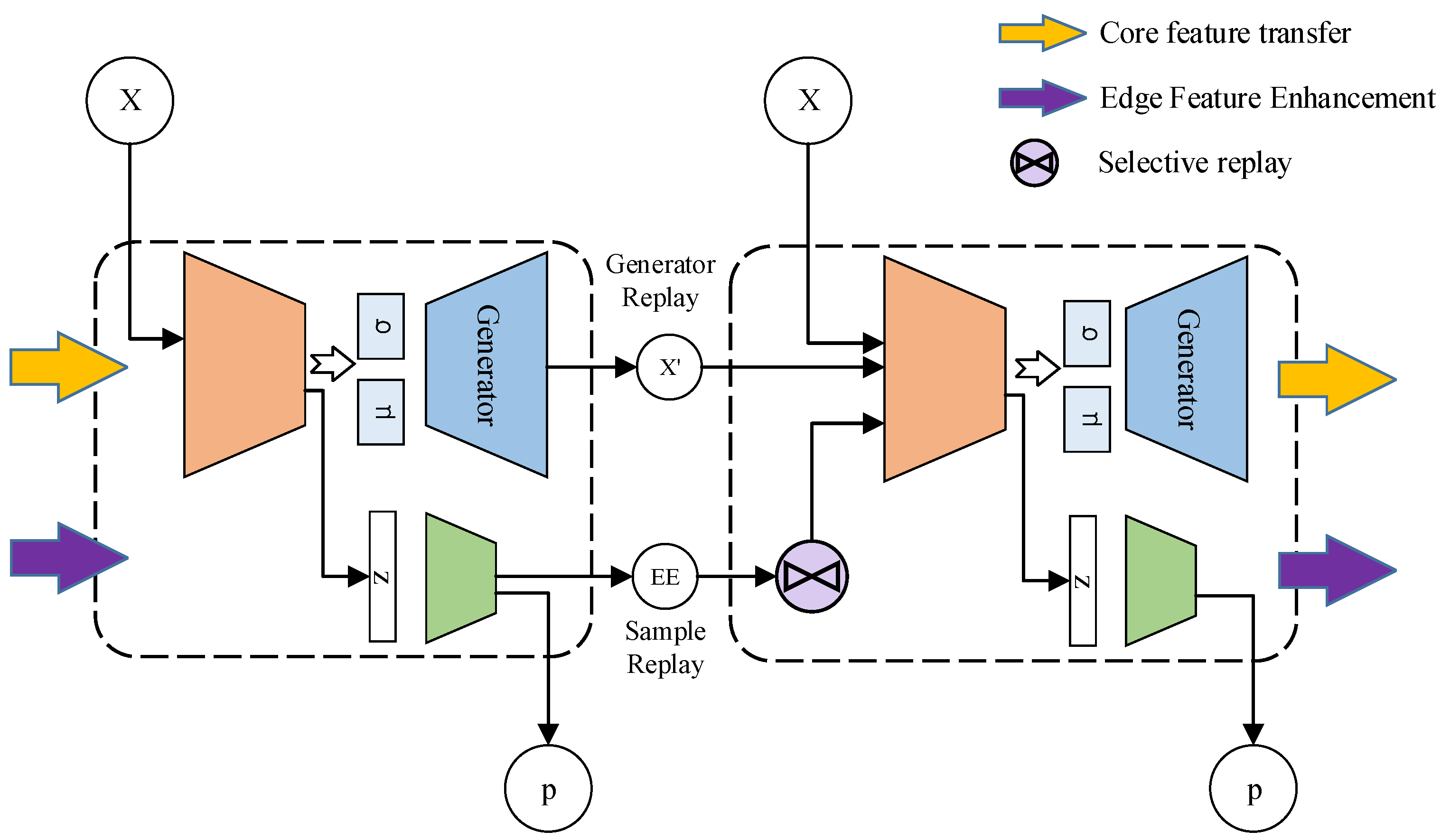
• A method named edge exemplar enhancement is proposed to optimize the increment learning framework. It enhances the memory of incremental learning on the edge of information from previous classes, and it effectively improves the recognition performance of replay-based incremental learning models.
• Based on public datasets and self-capture datasets, we simulated the iterative process of Tor traffic obfuscation technology in an experiment to verify the proposed model in this paper. The experimental results demonstrate the performance of the incremental learning framework for Tor-obfuscated traffic, and they also verify the effectiveness of edge exemplar enhancement.

The organization of this paper is as follows. Related work on obfuscated traffic detection is introduced and summarized in Section 2. In Section 3, we introduce the incremental learning framework and edge exemplar enhancement proposed in this paper. In Section 4, experiments are designed to verify the effectiveness of the proposed model compared with similar models. Finally, the results of this paper are summarized and future prospects are proposed.

2. Related Work

Early anonymous communication traffic identification was implemented based on some classic traffic identification methods, such as port-based, DPI, etc. When the traffic obfuscation technology was imperfect, DPI could also be used for its traffic detection, even though it used TLS encryption. There is some fixed pattern in the plaintext characteristics of its handshake phase. However, traffic obfuscation technology has patched these vulnerabilities, such as using ECC (elliptic curve cryptography) in obfs4 to encrypt TCP payloads and perform random padding. The emergence of traffic obfuscation technology makes it difficult for traditional traffic identification methods to effectively detect Tor anonymous communication traffic.

In order to combat the detection difficulties brought by traffic obfuscation techniques, a large number of researchers use machine learning and deep learning methods to identify anonymous communication traffic. Wang [4] divided Tor anonymous communication identification into three levels. The first level is the identification of anonymous traffic (L1). At this level, researchers mainly explore how to mine anonymous communication traffic from massive background traffic, such as Tor and I2P. The second level is the identification of traffic types. At this time, researchers focus on the further analysis of anonymous communication traffic, mainly discussing the identification methods of its communication behavior, such as video, FTP, VOIP, etc. The third level is the identification of anonymous traffic and applications. At this level, the traffic will be identified in a more detailed manner, as will the applications from which the communication behavior in L2 is mined. The above three levels cover the current main research direction of anonymous communication traffic. However, for Tor traffic identification, the detection of obfuscated traffic is not included. In this paper, we divide anonymous traffic identification into four levels. As shown in Figure 1, we add the traffic identification of different traffic obfuscation plugins of Tor as L2. This forms the four-level identification of Tor: L1 for anomaly traffic, L2 for obfuscation type, L3 for traffic type, and L4 for applications.

Based on the above divisions, this paper summarizes related work in Tor traffic identification. Some related works are summarized in the

Table 1. Research on Tor traffic detection in recent years.

Year	Features	Model	Dataset	PTs	Evaluation	Level
2018 [7]	TR&NTR	Mixture of Gaussian, Hidden Markov Model	self-captured	Meek	acc (99.98%) F1 (99.72%)	L2
2018 [8]	NTR	SVM, Adaboost, C4.5, Random Forest	self-captured	Obfs3 ScramleSuit Obfs4	auc (0.99%+)	L2
2019 [9]	NTR	Two-level filter	self-captured	Obfs4	pre (98.83%) FPR (00.03%)	L2
2020 [10]	TR	GBDT, XGboost, LightGBM, et al.	self-captured	–	acc (L1-96.9%, L3-91.6%)	L1, L3
2020 [11]	TR&NTR	Denoising Adversarial Autoencoder	self-captured	–	recall 83.7%	L2
2020 [4]	TR&NTR	Naïve Bayes, Bayes networks	self-captured	–	acc (mobile 96%+, PC 98%+)	L1, L3, L4
2021 [12]	TR&NTR	XGBoost, GBDT, Random Forest, CART	self-captured	Meek Obfs4 FTE	acc (99%+)	L2
2021 [13]	TR&NTR	TSCRNN	ISCXTor2016	–	acc (Tor 99.4%, nonTor 95.0%)	L1
2022 [14]	TR&NTR	XGBoost, SVM, Random Forest, KNN	self-captured	Snowflake	acc (99%+), F1 (98%+)	L2

. First of all, the Tor traffic detection target of L1 is to detect the target Tor traffic from the massive background traffic. Thus, it demands high efficiency for traffic detection and also needs to ensure that the model has a high true positive rate (TPR) and a low false positive rate (FPR). It focuses on utilizing traditional machine learning models with high recognition efficiency [5,6].

The L2 level is for the identification of Tor-obfuscated traffic. A large amount of research focuses on the identification of obfuscated traffic based on machine learning and deep learning. However, the input of the model relies on human analysis and designed features. For example, Yao [7] analyzed Meek-based Tor traffic flow. Their research shows that meek traffic has status features in the two dimensions of inter-packet time and packet size. Then, a MGHMM model was designed to mine the transition probability chain of the status feature. He [9] analyzed Obfs4-based Tor traffic flow. Since Tor uses ECC for encryption, all data packet payloads are encrypted and randomly padded. A coarse-grained detection method including random detection and packet length filtering is proposed for  fast detection of Obf4-based Tor traffic. Then, an SVM model is trained with the flow statistical characteristics for fine-grained detection.

Artificially designed traffic features bring more effective detection, but the labor cost is high, and the designed characteristics have limitations. Considering that Tor has many different types of PTs, many researchers have explored the possibility of using general statistical features to identify different types of Tor-obfuscated traffic. Wang [4] summarized the common flow statistical features in traffic identification. All features can be divided into two types: time-related features (TR) and non-time-related features (NTR). TR includes flow duration, interval time features, bytes or packets per second, etc. And NTR includes packet and byte counting, TCP headers, packet length, etc. It is worth mentioning that they discussed the differences between PC and mobile detection. Mohammad [8] directly used the flow statistical features extracted by Netmate. In order to ensure the real-time performance of recognition, they only perform feature extraction on the first 50 packets of each flow. Adaboost and traditional random forest were utilized as detection models.

With the development of machine learning and deep learning, neural networks have been verified to be more efficient in terms of feature extraction and recognition than traditional machine learning models. In many studies, neural networks are also used as a method for Tor-obfuscated traffic detection. Salman [11] proposed an obfuscated traffic detection method based on a denoising autoencoder. Their work explored different randomized obfuscation methods, including random padding and random inter-arrival time (IAT). Li [15] studied the C2 communication traffic of botnets using domain fronting technology. They proposed a recognition method based on convolutional neural networks (CNN). Their experiment verified the effectiveness of CNN for Meek-based Tor traffic identification.

L3 and L4 are in-depth analyses of Tor traffic identification. Its purpose is to further trace the source of Tor traffic from the behavior of the flow. Therefore, it is usually treated as a multi-classification problem. For example, there are seven common types of L3 based on user online behavior [16], including web browsing, p2p, etc. And there are more types of L4, which can reach dozens or even hundreds of types according to different applications. It is precisely because of these types that these two levels of traffic identification have higher requirements on the feature extraction and identification capabilities of the model, and complex neural networks have become the main model for their detection. Lin [13] proposed a model called TSCRNN, which has a recognition accuracy of 95% on 16 categories (L3) of Tor traffic. Shapira proposed Flowpic [17,18], a method that converts traffic into pictures. They used CNN to identify traffic behavior types, and even applications (L3&L4), with an accuracy rate of 99.7%.

As summarized above, there are many studies on detection methods for Tor-obfuscated traffic. However, the proposed detection methods usually only target one or more obfuscation techniques, as shown in Table 1. In this paper, we believe that the specificity of Tor-obfuscated traffic identification is manifested in the confrontation between detection and obfuscation, which should be a more dynamic process, and that the L2 identification model needs to be dynamically expanded to cope with the update of obfuscation techniques. This is also the motivation for this paper to propose an incremental learning framework for Tor-obfuscated traffic detection. However, to the best of our knowledge, there are few obfuscated traffic detection models for Tor’s PT based on incremental learning. Therefore, this paper takes this as a starting point to study and analyze the feasibility and recognition performance of incremental learning applied to dynamic Tor-obfuscated traffic detection.

3. Method

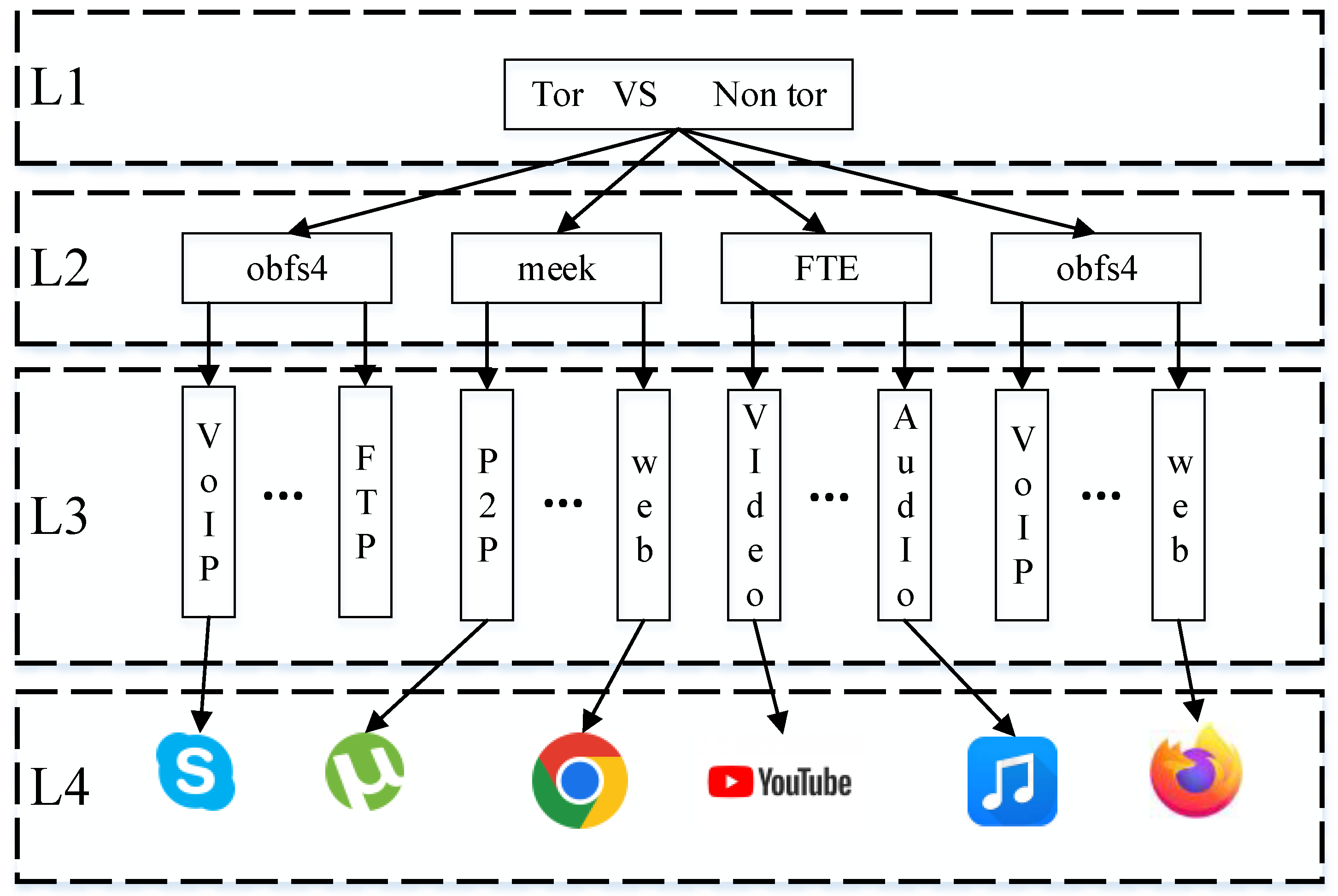
3.1. Tor Pluggable Transports

At present, three types of PTs—Obfs4, Meek, and Snowflake—are most commonly used in Tor and their work principles are shown in Figure 2. Obfs4 uses high-efficiency ECC encryption. When the TCP handshake ends, the client sends an obfs4 handshake request, including generating a Curve25519 key pair and sending the public key to the server. The server receives the request, performs authentication, and then sends the server’s public key to the client to complete the key negotiation. This process allows Tor to encrypt communication data using the negotiated key. Meek uses domain fronting techniques to obfuscate traffic. The principle of domain fronting technology is to use different domain names in different communication layers. Meek has a built-in front server, which is a web server provided by cloud service providers such as Akamai or Cloudfront. When a user tries to connect to the Tor network, the client encapsulates the Tor request into TLS, and then sends it to the front server. The front server unpacks this request and sends it to the Tor routing node. Therefore, the communication traffic observed by the censor is the TLS connection from the client to the front server, which is easily misjudged as normal web browsing behavior. Snowflake configures clients as proxies. After starting Snowflake, the local client will connect to a broker hosted on a cloud service provider protected by domain fronting. The broker will provide the established Snowflake proxy client (remote client), and the remote client will be utilized as a proxy to establish a WebRTC connection with the local client to access the Tor network. Therefore, the Snowflake traffic observed by the censor is WebRTC communication between two clients, which can easily be misjudged as a normal voice or video call between two users.

There are huge differences in the communication process of the above obfuscated method, so the detection features exposed by various obfuscation methods are also different, and most of them are protocol-related features, such as the protocol fingerprints of TLS and DTLS. This is also the reason why most studies only detect a single obfuscation technique. However, current incremental learning models require samples from different categories to have the same set of features. Therefore, the Tor-obfuscated traffic detection model based on incremental learning first needs to construct a feature set that can be used for a variety of different obfuscated traffic. So, in this paper, the general statistical characteristics of traffic extracted from the transport layer are taken into account when building the Tor-obfuscated traffic detection feature set.

The first and most common is randomization, and its representative is the Obfs series PTs. This type of traffic obfuscation method has a strict authentication mechanism. Based on this feature, He [9] designed timing detection as a filtering method. In this paper, we believe that the strict authentication mechanism will bring additional transmission delay, which may expose detection features on IAT, so we take the statistical features of IAT as an important component of traffic features. Second, Obfs4 has random padding and IAT-mode split data packets. The bytes of this padding can reach 8000+ at most. This will cause obfs4 streams to have a more random sequence of packet lengths than other types of obfuscated traffic. Another type of randomization obfuscation exists in Tor, known as connection padding. Connection padding disrupts communication behavior by inserting extra data traffic into the stream, making all traffic on the network appear to be of the same size and pattern. Making it impossible for an attacker to identify real communications through time intervals and transmission patterns. Therefore, in this paper, the information entropy of the packet length and the statistical characteristics of the packet length are also included in the traffic characteristics. In particular, the information entropy of the packet length is calculated as follows. We divide the packet length into 16 levels and take the MTU as the limit. We take the length mod100 of a length less than 1500 bytes as the result and divide all the lengths greater than 1500 into one level to construct a random variable L.

$$L=\left\{\begin{array}{c}l\mathrm{mod}100ifl/100<15\hfill \\ 15ifl/100\ge 15\hfill \end{array}\right.$$

(1)

After calculating the L, $p_i$ is the occurrence frequency of the i-th level L. The information entropy of the packet length is calculated by the following formula.

$$H=\sum _i-p_i\log p_i$$

(2)

Next is tunneling. Both Meek and Snowflake can be classified into this type. The core technology of Meek is domain fronting. Generally speaking, the server is not allowed to actively push data to the client, so the client using Meek needs to constantly poll the front server. During the communication process, there will be a large number of data packets polled by the client. These data packets are characterized by frequent appearances in the forward direction, and the packet length is small. Therefore, in the traffic characteristics, we additionally added the mode of packet length in the bi-direction, as well as other statistical features, such as maximum and minimum values. The Snowflake establishes connections based on WebRTC and DTLS. Therefore, in terms of feature design, we build a differentiated feature set from the perspective of flow rate. We add features such as flow bytes per second and flow packets per second to the flow feature set.

The feature set used in this paper to extract features from traffic is shown in the

Table 2. The traffic feature set and its description.

Features	Description
duration	Slide window duration
min_iat, max_iat, mean_iat, low_quartile_iat, median_iat, upp_quartile_iat	Statistic Interval time features
fb_psec, fp_psec	Flow speed
min_pl, max_pl, mean_pl, low_quartile_pl, median_pl, mode_pl	Statistic packet length
numPktsSnt, numPktsRcvd, numBytesSnt, numBytesRcvd, maxPktSizeSnt, avePktSizeSnt, minPktSizeSnt	Statistic packet length with direction
Conversations	Number of requests and responses
PL_entropy	Information entropy of packet length

. We finally selected 24 different features for Tor traffic identification. The selected features are partly based on the features given in the literature [4], which analyzes and summarizes some features of Tor available on mobile and PC platforms. Its feature set includes time-related features such as duration and interval time features, as well as non-time-related features such as packet length and its statistical values. These features have been utilized to identify and classify Tor traffic on Mobile and PC Platforms. In addition, we implement some new features that are commonly used in encrypted traffic identification, including information entropy and conversations. Finaly, a sliding window is used to split the flow, and the features in the table are extracted from the window.

3.2. Increamental Learning

The incremental learning model is required to continuously gain new knowledge from a data stream. We assume that there are K training datasets of non-overlapping categories $\{T^1,T^2,\cdots T^K\}$, where $T^k=\{(x_i^k,y_i^k)\}$ represents the k-th incremental learning training data set, also known as the training task. In the process of learning the k-th task, only the current training data set $S^k$ can be used. The expected risk of the model is described as follows.

$$E_{\left(x_i,y_j\right)\sim T^1\cup \dots T^K}\left[\ell \left(f\left(x_i\right),y_i\right)\right]$$

(3)

The main challenge of incremental learning is how to solve the catastrophic forgetting problem. If the model is only focused on learning a new task, it will lead to a sharp decline in its recognition performance for previous tasks. Incremental learning needs to solve the problem of balancing learning new knowledge with retaining previous knowledge during training. It can be summarized into three categories according to different methods of combating catastrophic forgetting [19]: regularization, replay, and template classification.

Regularization is intended to protect previous knowledge by imposing constraints on the loss function of new tasks. Its representative algorithm is learning without forgetting (LwF) [20]. The LwF algorithm proposes the method of using knowledge distillation to protect previous knowledge and alleviate catastrophic forgetting. In LwF, the previous task model is saved as a teacher model. During the training process of the new task, LwF uses the previous model to predict new class samples and compares its output with the new model output to construct a distillation loss. The distillation loss is defined as the cross-entropy loss of the previous and new models on the old classes.

Template classification is used to preserve previous task knowledge by constructing exemplar sets. Its representative model is iCaRL [21]. iCaRL divides the network into a feature extractor and a linear classifier. In the training process, the previous model is used as a teacher model for knowledge distillation. However, they do not use the trained linear classifiers for classification. They believe that catastrophic forgetting comes from the fact that the classifier is updated as the feature extractor is trained. The mean value of the previous class will change with the training of the feature extractor. Using nearest-mean can make the classifier robust to feature representation changes. Therefore, exemplar sets are constructed based on the output of the feature extractor, and the mean value of the hidden space features of each class is used as a template to classify samples by nearest-mean-of exemplars.

Replay uses a generate model to store previous class knowledge. Its representative models are deep generative replay (DGR) [22] and brain-inspired replay (BI-R) [23]. In implementation, a generative model is trained for the simulated generation of previous class samples. When training a new task, the trained generative model generates samples based on the knowledge of the old task and combines the samples of the new task to train the model.

The incremental learning model based on replay has achieved state-of-the-art experimental results [19]. However, two issues are still worth considering. Can the generative model produce the samples that are distributed at the edges of the dataset? Hod can we supplement the knowledge that the generative model is difficult to generate or is gradually forgotten during the training process?

For the first problem above, the solution used by replay-based incremental learning models is to try to use some method to improve the quality of the generator. In DGR, WGAN-GP is used to improve the quality of the generated model. In BI-R, four brain-inspired techniques are proposed to improve the performance of the model. This paper considered that these methods only improve the quality of generated samples, making them more similar to real samples, and did not discuss the breadth of model data generation. Especially in traffic identification scenarios, there is a lot of sudden traffic, which is difficult to generate by models. We define these samples as edge exemplars.

Definition 1.

Edge exemplars are the collection of samples with a low probability of being predicted as ground truth.

Based on the above definition, the core challenge lies in the identification and construction of edge samples at each stage of the model training process. Suppose the current training stage involves data from n distinct categories. Let x denote a sample belonging to the k-th category. When x is input into the nueral network, it will produces an output vector $f(x)=(z_1,\dots ,z_k)$. The Softmax layer transforms the output vector into a probability distribution over the n categories using the Formula (4). This process yields the probability $p_i$ of the sample x belonging to each category i; $p_i=\mathrm{Softmax}(z_i)$. If x is correctly classified, the probability $p_k$ corresponding to its true label k will dominate the probabilities of all other categories.

$$Softmax(z_i)={\displaystyle \frac{e^{z_i}}{{\displaystyle \sum _{j=1}^K}{e}^{z_j}}}$$

(4)

Therefore, this paper proposes a method to identify edge samples as follows. First, the model is trained on the training dataset. Next, the training data are divided according to their true labels and fed into the nuerual network separately. For each category, the neural network generates a set of prediction probabilities for all samples. Specifically, for a sample belonging to the k-th category, its probability of being predicted as the k-th category is extracted. This result in a probability collection $P_k$ for all samples in the k-th category through Formula (5). Within this collection, a lower probability suggests reduced confidence; this means that the sample deviates from the core area of the k-th type marked by the neural network. Finally, we sort the prediction probabilities in $P_k$ and select the batch of samples with the smallest probability as edge samples.

$$P_k=\{Softmax(z_i^1),Softmax(z_i^2),\dots \}=\{p_k^1,p_k^2,\dots \}$$

(5)

In this paper, we beleive that the generative models can only replay some easily classifiable samples with key features. And some samples that are difficult to classify cannot be replayed by the generative model. If only the generative model is used for replay, the edge sample information in the training dataset will be lost during the incremental learning process, resulting in a decrease in model performance.

The method designed in this paper to solve the problem of edge information forgetting is to construct edge exemplar sets. Since the generative model can only generate samples with key features for replay, we try to directly collect samples that are misclassified during incremental learning to construct edge exemplar sets to enhance the memory of the model for previous classes. The improved Tor-obfuscated traffic incremental learning framework designed in this paper is shown in the Figure 3.

In application scenarios, the detection of Tor traffic changes dynamically. For example, in the early stages, it may only detect Tor traffic without obfuscation. With the update of Tor PTs, censors need to detect the traffic from different types of PTs, such as FTE and Meek. And it may even require the detection of Tor-obfuscated traffic on different clients (PC and Mobile). This dynamic process requires the model to have the ability to learn incrementally. On the one hand, it can reduce the storage pressure of previous types of data; on the other hand, it can avoid the need to retrain the model for new detection requirements. This will greatly reduce the computational requirements of the model.

In the incremental learning framework designed in this paper, it is mainly divided into three parts: feature extractor, incremental learning model, and edge exemplars. The feature extractor is used to convert communication traffic into numerical features. The feature set is defined in Table 2. The incremental learning models are trained according to different tasks. These tasks in Tor-obfuscated traffic detection include initial background traffic and non-obfuscated Tor traffic, the traffic of different Tor PTs, and even the traffic of different clients. The edge exemplars are some real samples extracted from the training dataset. These samples will be mixed with the generated samples as the input data for the following training process to enhance the memory of the previous class.

3.3. Edge Exemplars Enhancement

In this paper, the proposed method for enhancing edge sample memory during incremental learning is named edge exemplar enhancement, as shown in Figure 4. The yellow arrow in the figure is the previous class replay process of replay-based incremental learning. In the structure designed in this paper, we use two techniques to enhance edge sample information: edge feature enhancement and selective replay. 

The purpose of edge feature enhancement is to enhance the memory of edge sample features during the incremental learning process by replaying some real edge samples, thereby improving the ability to identify edge samples and reducing catastrophic forgetting during the training process. In incremental learning models like BI-R and DGR, the classifier uses knowledge distillation to improve the model’s memory for the old class. It does this by using the samples made by the generative model and the labels predicted by the previous model. The weight of real samples and replayed samples of the current training type is controlled by the parameter $\alpha$, as shown in Formula (6). The edge feature enhancement requires building an edge exemplar set of trained types of data during the training process and using these real samples and labels in subsequent training. Therefore, the objective function of the optimized model training is also divided into two parts, and a hyperparameter $\eta$ is used to adjust the weight of the two parts, as shown in the Formula (7).

$$\underset{w_i}{\arg \min }\alpha E_{x\in T_i}[L(x,f(x;w_i))]+(1-\alpha )E_{x^{\prime }\in X_{gen}}[L(x^{\prime },f(x^{\prime },w_{i-1}))]$$

(6)

The idea of edge feature enhancement comes from the category weight of dealing with data imbalance. On the one hand, edge samples should only occupy a small proportion of the total data. On the other hand, in order to reduce the amount of computation and storage resources, the number of real samples stored in the incremental learning model should be limited, such as the upper limit of samples in iCaRL. The size of the exemplar set should be much smaller than the training data. Therefore, in order to ensure that the replay of edge exemplars can effectively enhance the model, we give it a larger category weight $\eta$, which is the penalty factor, similar to cost-sensitive learning for imbalanced data.

$$\begin{array}{cc}\hfill \underset{w_i}{\arg \min }& \alpha E_{x\in T_i}\left[L\left(x,f\left(x;w_i\right)\right)\right]\hfill \\ \hfill & +(1-\alpha )E_{x^{\prime }\in X_{\mathrm{gen}}}\left[L\left(x^{\prime },f\left(x^{\prime },w_{i-1}\right)\right)\right]+\eta E_{\tilde{x}\in EE}[L(\tilde{x},\tilde{y})]\hfill \end{array}$$

(7)

Selective replay is a technique designed in this paper to replay edge exemplars. On the one hand, we consider that there is a small sample size of the edge exemplars, and we need to use bagging for sample replay during the replay process; wn the other hand, there are differences between the edge samples and the main data in this class. If the edge samples are replayed frequently, this may cause the model drift to affect the classification performance. Therefore, we utilized selective replay. Selective replay is divided into two steps. The first step is the bagging of batches. In order to avoid too many replay samples affecting the classification performance, we only replay edge exemplars in some batches of the training process. The second step is the bagging of edge exemplars. In the selected batch, we set $\gamma$ as the proportion of EE samples in the batch and then randomly sample from edge exemplars.

Based on the two incremental learning models of DGR and BI-R, this paper implements the edge sample replay algorithm. This paper has given the definition of edge samples in Definition 1. In replay-based incremental learning, the discriminative model from the previous task will be used as a teacher to carry out knowledge distillation on the model trained by the new task. Therefore, it is difficult for the classifier in the incremental learning process. The identified samples will be gradually forgotten as the work progresses, so the misclassified samples in each class can be regarded as marginal samples. Using edge feature enhancement to enhance the replay-based incremental learning algorithm is shown in Algorithm 1.

Algorithm 1 Replay-based incremental learning with edge exemplar enhancement

Require: The training dataset for the current task: $X_k,Y_k$, $Y_k=\{1,2,\dots ,c\}$; The Generator and classifier of previous task: $G_{pre}$, $C_{pre}$; Edge exemplars extracted by the previous $k-1$ tasks: $\mathrm{E}{\mathrm{E}}_{k-1}$; The proportion of EE samples replayed in a batch: $\gamma$; The size of the EE sampled for each class: m Ensure: $y=x^n$   1: Initialize the Encoder E, Decoder D and Classifer C, initialize parameters $w_{gen}$ and $w_c$, initialize hyperparameters learning rate, batchsize m, optimizer, etc.;   2: while Loss not converge do   3:     $x,y=DataLoader(X_k,Y_k)$   4:     Randomly sample the hidden variable $z^{\prime }$ to the labels to generate samples, $x_{gen}=G_{pre}(z^{\prime })$, $y_{gen}=C_{pre}(x_{gen})$.   5:     if Current batch is selected then   6:         $x_{ee},y_{ee}=Random\_choice(E{E}_{k-1},(1-\gamma \ast m))$   7:     else   8:         $x_{ee}=None$   9:     end if 10:     Merge all replayed samples, $x_{replay}=x_{gen}+x_{ee}$, $y_{replay}=y_{gen}+y_{ee}$ 11:     Forward propagation replays samples, $y^{\prime }=C(x)$, $\widehat{y}=C_{pre}(x_{replay})$, ${\widehat{y}}_{ee}=C(x_{ee})$ 12:     Calculate the current task loss, $L_{cur}(y,y^{\prime })$ 13:     Calculate the replay samples loss, $L_{replay}(y_{replay},\widehat{y})$ 14:     Calculate the edge exemplars loss, $L_{EE}(y_{ee},{\widehat{y}}_{ee})$ 15:     Backpropagation updates the weights, $w\leftarrow Adam(\alpha L_{cur}+(1-\alpha )L_{replay}+\eta L_{EE})$ 16: end while 17: The train dataset are divided into multiple data sets $\{D_1,D_2,...,D_c\}$ according to the true category labels, where $D_i=\{(x_j,y_j)|y_j=i\}$ 18: Calculate the predicted probability vector for each class, $\{C(D_1),C(D_2),...,c(D_c)\}$ 19: Extract the probability of each class of samples predicted as the true category through the Formula (5), and get $\{P_1,P_2,...,P_c\}$ 20: Calculate the distance between the predicted value and the label of each class, $P{C}_i=\{1-p_i^j|p_i^j\in P_i\}$ 21: select m samples with the largest distance as the edge exemplar, $E{E}_k\leftarrow E{E}_{k-1}+\{To{p}_k(P{C}_1),...,To{p}_k(P{C}_k)\}$ 22: return G, C, $E{E}_k$

In Algorithm 1, the input of the model includes the training data of the current task, the generated model trained by the previous task, and the edge exemplars constructed. In each epoch of training, the model first randomly samples some hidden vectors as the input of the generator to build replay samples. Based on selective replay, some epochs in the training process will be randomly selected. In the training process, if the current epoch is selected, we randomly sample from the edge exemplar set with a ratio of $\gamma$ for replay. At this time, the training sample of epoch includes three parts: the training sample x of the current task, the generator replay sample $x_{gen}$, and the replayed edge exemplars $x_{ee}$. Among them, both $x_{gen}$ and $x_{ee}$ are replay samples. After these three data parts are forward-propagated, the loss is calculated to obtain the loss $L_{cur}$ of the current task and the loss $L_{replay}$ of the replay sample, which correspond to the first two parts of Formula (7), respectively. At the same time, the penalty coefficient $\eta$ is used in the edge feature enhancement of this paper to enhance the memory of the classifier for the edge samples of the old class. Therefore, in the algorithm, we use the penalty coefficient $\eta$ to control the additional penalty term $L_{EE}$ of the edge exemplars, as shown in Formula (7). In the third part, we calculate the sum of the three parts of the loss according to the predefined weights $\alpha$ and $\eta$ and then perform backpropagation through the Adam algorithm [24] to complete the incremental learning model training under edge exemplar enhancement. Finally, edge exemplars of all classes in the current task are constructed. In this paper, the misclassified samples in each class are used as edge samples, but the softmax output is the probability of the sample, so we use the k samples with the largest difference between its predicted probability and its true label. These samples are retained as edge exemplars.

The above algorithms can be applied to DGR and BI-R at the same time. But there are certain differences in the process of application. First of all, in the selection of the generation model, DGR uses WGAN-GP to generate and replay samples [25], while BI-R uses variational autoencoders (VAE) [26]. The generator and discriminator in DGR are defined separately, so the loss calculated by the algorithm only includes the Solver’s loss, and its loss is a cross-entropy function, which is defined as Formula (8).

$$L_{cur}=CE(y,y^{\prime })=-{\displaystyle \frac{1}{N}}\sum _{i=1}^n\sum _{j=1}^{N_k}{y^{\prime }}_{ij}\log \left(p_{ij}\right)$$

(8)

The calculations of $L_{replay}$ and $L_{ee}$ also use cross-entropy. Its calculation method is the same as Formula (9).

$$L=\alpha CE(y,y^{\prime })+(1-\alpha )CE(y_{replay},\widehat{y})+\eta CE(x_{ee},{\widehat{y}}_{ee})$$

(9)

However, a trick named replay through feedback is used in BI-R; the Softmax layer is added as a classifier after the penultimate layer of the encoder of VAE, so the training of the generator and the incremental learning classifier are performed simultaneously, which also leads to differences in the loss calculation. The loss in BI-R includes the loss of VAE training.

$$L_{cur}={\lambda }_{rec}{L}_{rec}(x,x_{rec})+{\lambda }_{latent}{L}_{latent}(x)+{\lambda }_{dill}{L}_{dill}(y,y^{\prime })$$

(10)

It contains three parts, the first part $L_{rec}$ is the reconstruction loss of VAE, the second part $L_{laltent}$ is the KL divergence between the hidden empty vector and the normal distribution during the VAE training process [26]. The third part is the cross entropy between predicted value and its real label. These three parts are calculated as follows.

$$L_{recon}(X,X_{recon})={\displaystyle \frac{1}{n}}\sum _{i=1}^n{∥X-X_{recon}∥}_2$$

(11)

$$L_{latent}(x;\varphi )={\displaystyle \frac{1}{2}}\sum _{j=1}^{N_k}\left(1+\log \left({\sigma }_j^2\right)-{\mu }_j^2-{\sigma }_j^2\right)$$

(12)

$$L_{dill}=CE(y,y^{\prime })=-{\displaystyle \frac{1}{N}}\sum _{i=1}^n\sum _{j=1}^{N_k}{\tilde{y}}_{ij}\log \left(p_{ij}\right)$$

(13)

The loss calculation of the replay sample also includes these three parts, but the purpose of the wdge feature enhancement proposed in this paper is to strengthen the ability to recognize edge exemplars without having a large impact on the generator trained by the current task. Therefore, $L_{ee}$ is listed separately in the algorithm to strengthen the ability of the classifier to recognize edge exemplars.

Finally, backpropagation is performed based on the calculated loss. $\alpha$ is usually set to the proportion of newly added categories, that is, the ratio of the number of categories in the current task to the number of all categories known by the incremental learning model. But $eta$ needs to be adjusted manually, and we analyzed it in the experiment.

In addition, it is worth mentioning that BI-R proposes four brain-inspired techniques to improve the quality of sample generation on the basis of DGR: replay through feedback, that is, adding a Softmax layer after the penultimate layer of the VAE encoder as a classifier; conditional replay, that is, replacing the standard normal distribution of VAE’s latent variable with a GMM model so that each class has a specific pattern in the hidden space; gate based on internal context, that is, adding gates to different layers of the neural network control so that it can be adapted to specific tasks; and internal replay, which achieves replay at the hidden feature level by freezing the convolutional layer. In this article, we use BI-R to detect Tor-obfuscated traffic, whose input has been feature extracted so we can replay the input as a hidden feature. In the implementation process of this article, we selectively discarded the internal reply technique in BI-R.

4. Experiment

4.1. Data Collection

In order to simulate the changes in demand for Tor-obfuscated traffic detection. The dataset in this paper utilized public datasets and self-collected data. The public dataset is utilized as the historical version of Tor traffic, and the self-captured data contains the traffic of Tor built-in PTs in the latest version, including Obfs4, Meek, and Snowflake.

We organize these datasets as follows: T0-ISCXTor2016 [16], which collects seven types of background traffic and Tor traffic, such as chat and mail; T1-Old version Tor browser-obfuscated traffic [12], which contains three types of obfuscated traffic, including FTE, Meek, and obfs4; and T2-mobile Tor traffic [27], which provides traffic generated by Orbot, an application for mobile access to the Tor network [27]. These data use the technology of Tor connection padding to obfuscate traffic. It inserts additional data traffic into the communication on the Tor network, making the network traffic pattern more difficult to analyze and identify. It includes two kinds of padding: orbot padding and orbot reduce padding. Meanwhile, we collected the Tor browser traffic on the mobile terminal, and the obfuscation type is Snowflake. It served as a supplement to obfuscate Tor traffic on mobile. T3 refers to the traffic of the latest version of the Tor Browser. This part of the traffic is self-collected. It contains three types of traffic, including Meek, obfs4, and Snowflake. It intersects with the data in T2, so we configured a proxy in the Tor browser. We mark these types as proxied-Meek and proxied-obfs4.

The process of all data generation and collection is shown in Figure 5. First, when collecting mobile traffic for T2, we use the tested mobile phone to connect to the hotspot on the PC. Then, we start Wireshark on the personal computer to capture the communication traffic. When collecting the Tor Browser traffic for T3, we rented a cloud server as a proxy node. We collect Tor browser traffic between personal computers and proxy servers. All of the above self-collected traffic comes from two online behaviors: web browsing and video. In order to ensure the collection of pure Tor browser traffic. When the collection is complete, we filter the traffic according to the server IP to ensure the purity of the collected data. Finally, the data used in the experiment are shown in the

Table 3. The data size and content of each task.

Task ID	Content	Data Size and Type
T0	Background traffic flow and non-obfuscated Tor traffic	9.87 GB background 11.3 GB Tor Non-obfs
T1	Tor obfuscated traffic flow	12.9 GB FTE 8.43 GB Meek 13.5 GB Obfs4
T2	Mobile Tor traffic	1.32 GB orbot_pd 1.30 GB orbot_rpd 0.9 GB Mobile Snowflake
T3	Proxied Tor obfuscated traffic and Snowflake	0.9 GB proxied-Meek 2.55 GB proxied obfs4 3.86 GB PC Snowflake

.

4.2. Evaluation Metrics

In the experimental part of this paper, we utilized the following metrics to evaluate the model. There are used to verify the performance and efficiency of the incremental learning framework proposed in this paper to detect Tor-obfuscated traffic.

Intra-task evaluation. The main purpose of intra-task evaluation is to show the changes in the detection performance of all categories during the training process, which is also the usual evaluation of multi-classification problems. It can be evaluated through a confusion matrix. In the confusion matrix, each row represents the ground truth, and each column represents the type of model prediction. The elements in the confusion matrix are the number of samples, as shown in

Table 4. Confusion matrix.

	Class1	Other Classes
Class1	TP	FN
Other classes	FP	TN

.

The confusion matrix derives multiple evaluation indicators for multi-classification models, including FPR, precision, and recall. This paper uses these indicators to demonstrate the identification ability of the incremental learning model in each class.

$$precision={\displaystyle \frac{TP}{TP+\mathrm{FP}}}$$

(14)

$$recall={\displaystyle \frac{TP}{TP+FN}}$$

(15)

$$FPR={\displaystyle \frac{FP}{FP+TN}}$$

(16)

At the same time, we use the accuracy to analyze the overall performance of the model.

$$accuracy={\displaystyle \frac{TP+FN}{TP+TN+FP+FN}}$$

(17)

Inter-task evaluation. The purpose of inter-task evaluation is to show the recognition of the model on different tasks after each new task is added during the incremental learning process. In the experiment, we divided the data into four tasks to test the incremental learning model. Therefore, indicators for each stage of incremental learning are also necessary. Therefore, we sum the sample sizes belonging to the same task in the confusion matrix to obtain a new confusion matrix for evaluation. For example, $M_{task}[i,j]$ indicates that the number of samples whose real label belongs to the i-th task is predicted as the class of the j-th task, as shown in Formula (18).

$$M_{task}[i,j]=\sum _{k\in tas{k}_i}\sum _{l\in tas{k}_j}M[k,l]$$

(18)

The evaluation index derived from the task confusion matrix is the same in the Formulas (14)–(17).

4.3. Network and Parameter Settting

The neural network structure settings in the experiment are shown in

Table 5. The layer setting in neural network.

Layer	Setting
Linear	Input_dim = 31, output_dim = 64, active = LeakyReLU
Linear	Input_dim = 64, output_dim = 128, active = LeakyReLU
Linear	Input_dim = 128, output_dim = 128, active = LeakyReLU
Linear	Input_dim = 128, output_dim = 11

. Four fully connected layers are utilized in the network. We selected LeakyReLU as the activation function and the Adam algorithm as the gradient descent method.

Other parameters and their descriptions during the experiment are shown in the

Table 6. The hyperparameter setting in neural network.

Hyperparamter	Describe	Value
Epochs	Train epochs	100
lr	Learning rate	0.001
Batchsize	Batch size	256
${\beta }_1,{\beta }_2$	Adam optimizer parameter	0.9, 0.999
m	Edge exemplars size per class	100
$\eta$	The proportion of edge exemplars in the batch	0.1
$\gamma$	Edge feature enhengcement weight	2.0
${\lambda }_{recon},{\lambda }_{latent},{\lambda }_{dill}$	The weight of each loss function	1.0, 1.0, 1.0

.

4.4. Evaluation

First, we compare our model (DGR-EE, BI-R-EE) with the other incremental learning models. The baseline model for comparison is as follows: The joing tain uses all the data up to the current task to retrain the model. Therefore, joint training is also considered the upper bound of incremental learning. LwF [20] is a representative model of regularization-based incremental learning. It uses knowledge distillation to preserve previous class knowledge. ICaRL [21] is a representative model of template-classification incremental learning. It stores a small number of samples as an exemplar set and uses its mean as a template for classification. DGR [22] and BI-R [23] are representations of replay-based incremental learning. They use GAN or VAE to generate samples and replay them to alleviate catastrophic forgetting.

Overall evaluation. The first is the recognition accuracy of the model with respect to each class, as shown in Figure 6a. The BI-R-EE has achieved recognition ability second only to the joint train in most classes. By employing the edge exemplar enhancement, DGR and BI-R have significantly improved the recognition accuracy of non-obfs, Meek, PC Snowflake, and other types. For example, the recognition accuracy of non-obfs is 0.9955 (BI-R-EE), 0.9824 (BI-R), 0.9769 (DGR-EE), and 0.9087 (DGR). Figure 6b shows the mean value of difference evaluation metrics for all classes, including accuracy, precision, recall, and FPR. It is arranged according to accuracy from large to small. The metrics of BI-R-EE are the closest to those of the joint train. But it has obvious shortcomings in precision, which is due to the misclassification caused by previous class knowledge forgotten during training. Figure 6c shows the test accuracy up to the current task during the training process. Replay-based incremental learning shows the most gradual drop in test accuracy. Meanwhile, with the use of edge exemplar enhancement, the problem of test accuracy drops in the incremental learning process is further alleviated.

Intra-task evaluation. In intra-task performance evaluation, the type recognition offset within each task is also an important evaluation index.

Table 7. The identification accuracy of each task and the overall accuracy rate of the incremental learning model after training.

	Task0	Task1	Task2	Task3	Total
Joint	0.9992	0.9354	0.8651	0.9986	0.9437
LwF	-	-	-	0.998	0.1066
iCaRl	0.9899	0.6428	0.9311	0.9984	0.3279
DGR	0.9826	0.8511	0.4805	0.9988	0.5049
DGR-EE	0.9486	0.7261	0.7236	0.9984	0.7187
BI-R	0.9951	0.8651	0.8418	0.9988	0.8476
BI-R-EE	0.9952	0.8245	0.7773	0.9988	0.8767

precisely shows the differences between all models in task accuracy. In terms of total accuracy, BI-R-EE is the closest to the joint train, with a recognition accuracy of 87.76%. From the results shown in the table, the accuracy of BI-R on each task is greater than that of BI-R-EE, but its total accuracy is 3% lower than that of BI-R-EE. This is caused by the information loss problem of edge samples. The generative models used in DGR and BI-R well maintain the difference in type distribution within tasks, so the recognition accuracy rate within each task is relatively high, but as incremental learning progresses, the edge information of samples in the old class is lost, so many edge samples in previous tasks are misclassified, so the overall accuracy rate will be lower than the model using the edge exemplar enhancement method. The purpose of the edge exemplar enhancement proposed in this paper is to reduce misclassification between tasks. However, replaying edge exemplars will cause the model’s decision-making surface to shift, so the accuracy of intra-task classification will decrease slightly.

Inter-task evaluation. In this paper, through the edge exemplar enhancement method, we expect to enhance the memory of the previous task and reduce the inter-task bias. We compare our model with its baseline model to reveal the effectiveness of the edge exemplar enhancement for reducing inter-task bias that is proposed in this paper. We use Formula (18) to calculate the confusion matrix of each task in the incremental learning process. The result is shown in Figure 7. The data in each square represent the proportion of the data in that part. This figure shows the details of the knowledge forgetting of the previous task before and after using edge exemplar enhancement. Both DGR and BI-R misclassified a large number of previous task samples into the following tasks. In particular, DGR misclassified 26.3% of the samples from T1 into T3. BI-R also misclassified 4.1% of samples from T1 into T3. After edge exemplar enhancement, these values are reduced from 26.3% to 5.1% and from 4.1% to 0.31%, respectively. This also verifies the effectiveness of the edge exemplar enhancement proposed in this paper.

The above analysis and results show that the edge feature enhancement and selective replay designed in this paper introduce extra intra-task bias after replaying edge samples, reducing the recognition accuracy within the task but increasing the overall recognition accuracy. The reason is that edge exemplar replay can reduce inter-task bias. We think this is meaningful. On the one hand, the overall performance of the model has improved. On the other hand, the recognition accuracy of intra-task can try to use an additional model to identify a certain Task type alone, thereby achieving performance improvement. The recognition accuracy of tasks is difficult to improve through this method, because it needs to concatenate the types in multiple tasks, which is close to joint training.

Moreover, analysis of the confusion matrix reveals persistent knowledge forgetting in the incremental learning process. A significant portion of samples from previous tasks is misclassified as belonging to the most recent task. This problem deserves further study. For instance, confidence-based calibration can be employed to adjust the temperature parameter using old category data, thereby making the model’s predictions for previous tasks more conservative. This approach may reduce the misclassification of old task samples and enhance overall model robustness.

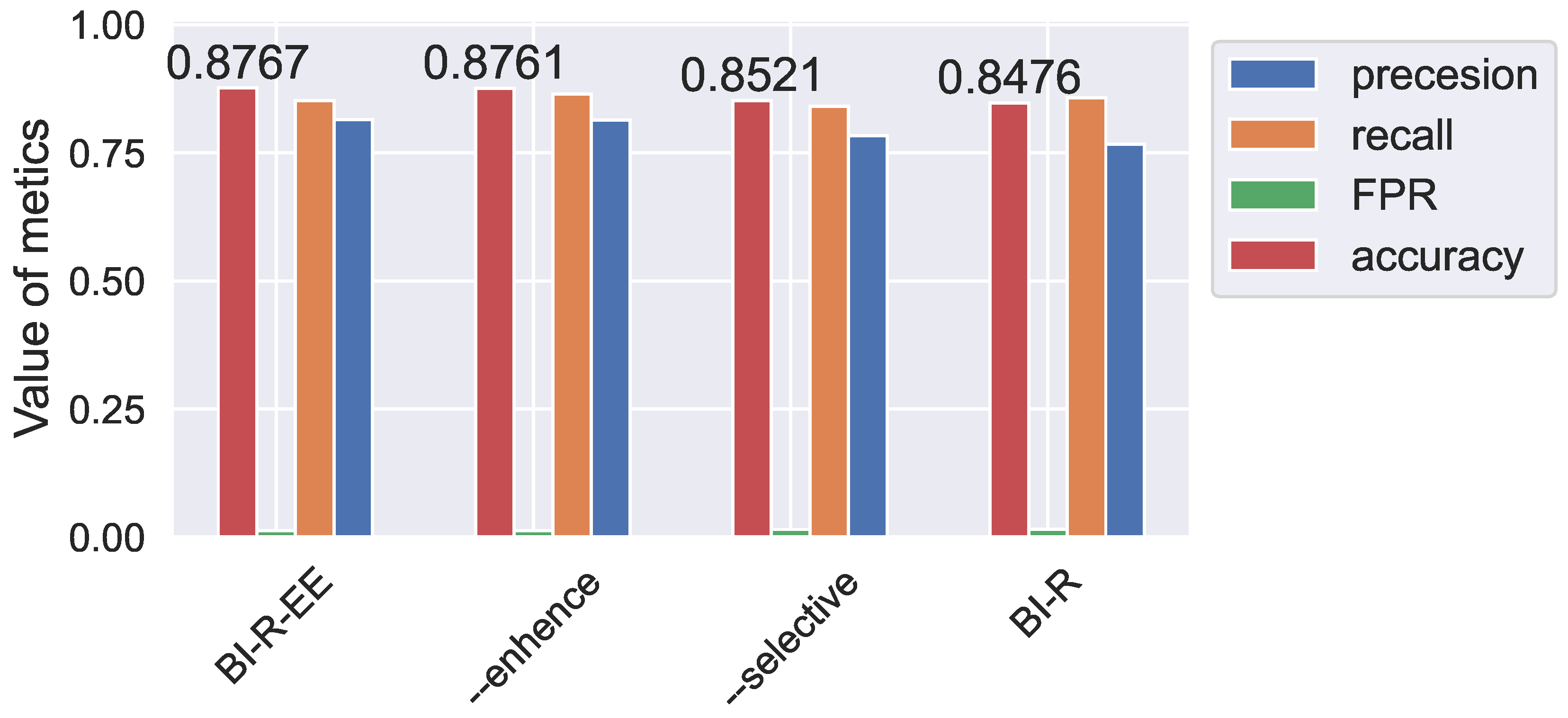
4.5. Ablation Experiment

In this paper, we conducted ablation experiments on the two edge exemplar enhancement techniques to verify their effectiveness in enhancing the performance of the model. In this article, our two techniques are edge feature enhancement and selective replay. Therefore, we control the variables to show the effectiveness of the edge information enhancement and selective replay proposed in this paper, respectively. In this part of the experiment, we set up four groups of models separately: BI-R, BI-R with edge feature enhancement, BI-R with selective reply, and BI-R-EE. The experimental results are shown in Figure 8. When the two techniques are not used, that is, the initial BI-R model, the overall recognition accuracy rate is 84.76%. After adding edge feature enhancement, the recognition accuracy of the model increased to 85.21%. After adding selective replay, the recognition accuracy of the model increased to 87.61%. When the two techniques are used simultaneously, namely, BI-R-EE, the recognition accuracy reaches a peak of 87.67%. This change in accuracy shows the effectiveness of edge feature enhancement and selective replay. From the perspective of the performance impact on the model, selective replay is more effective.

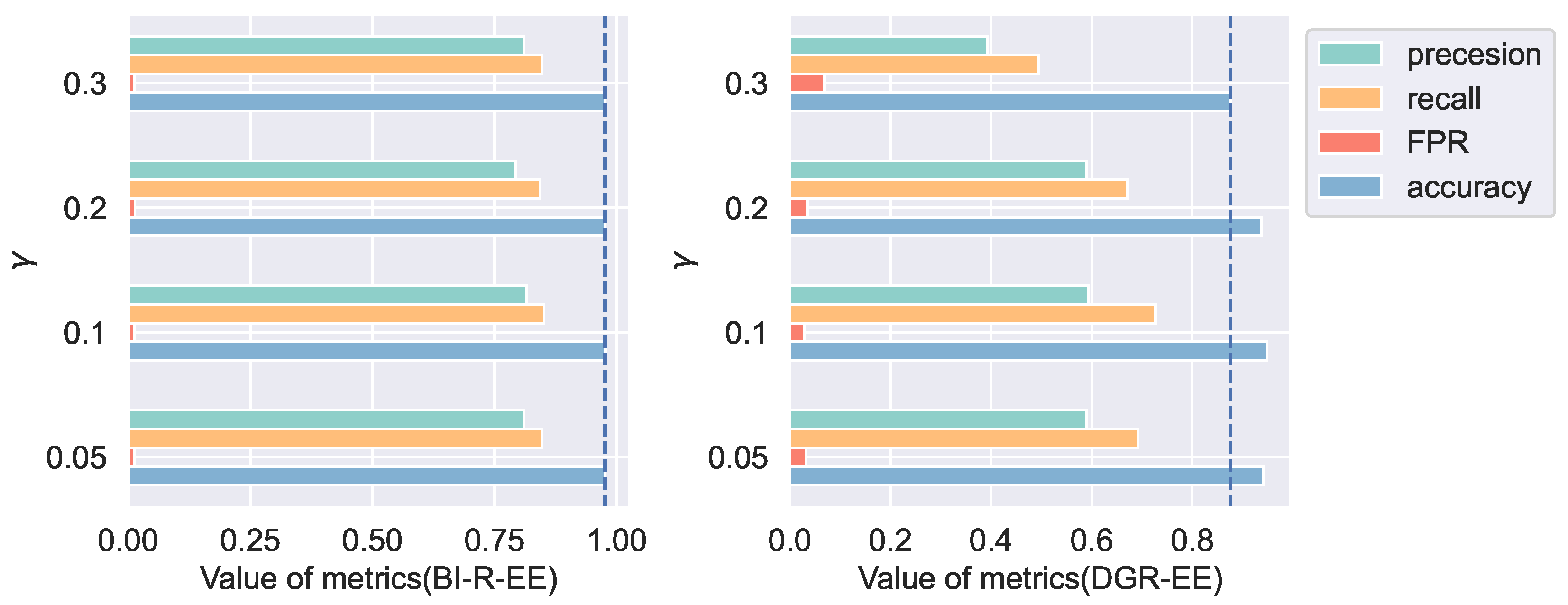
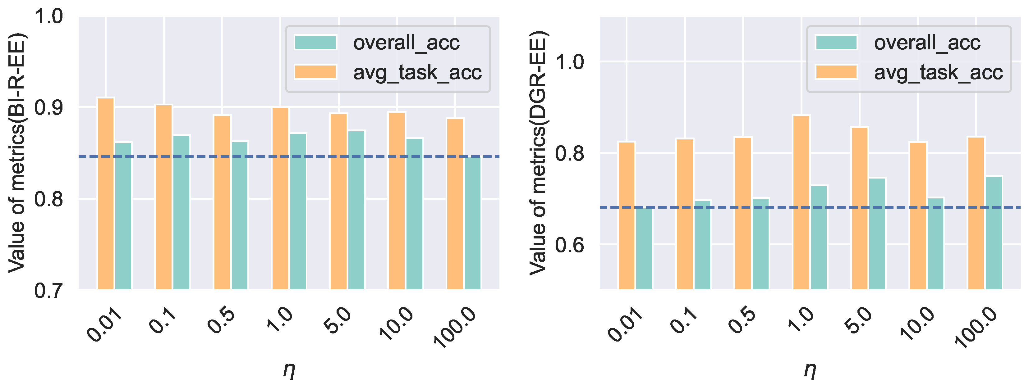
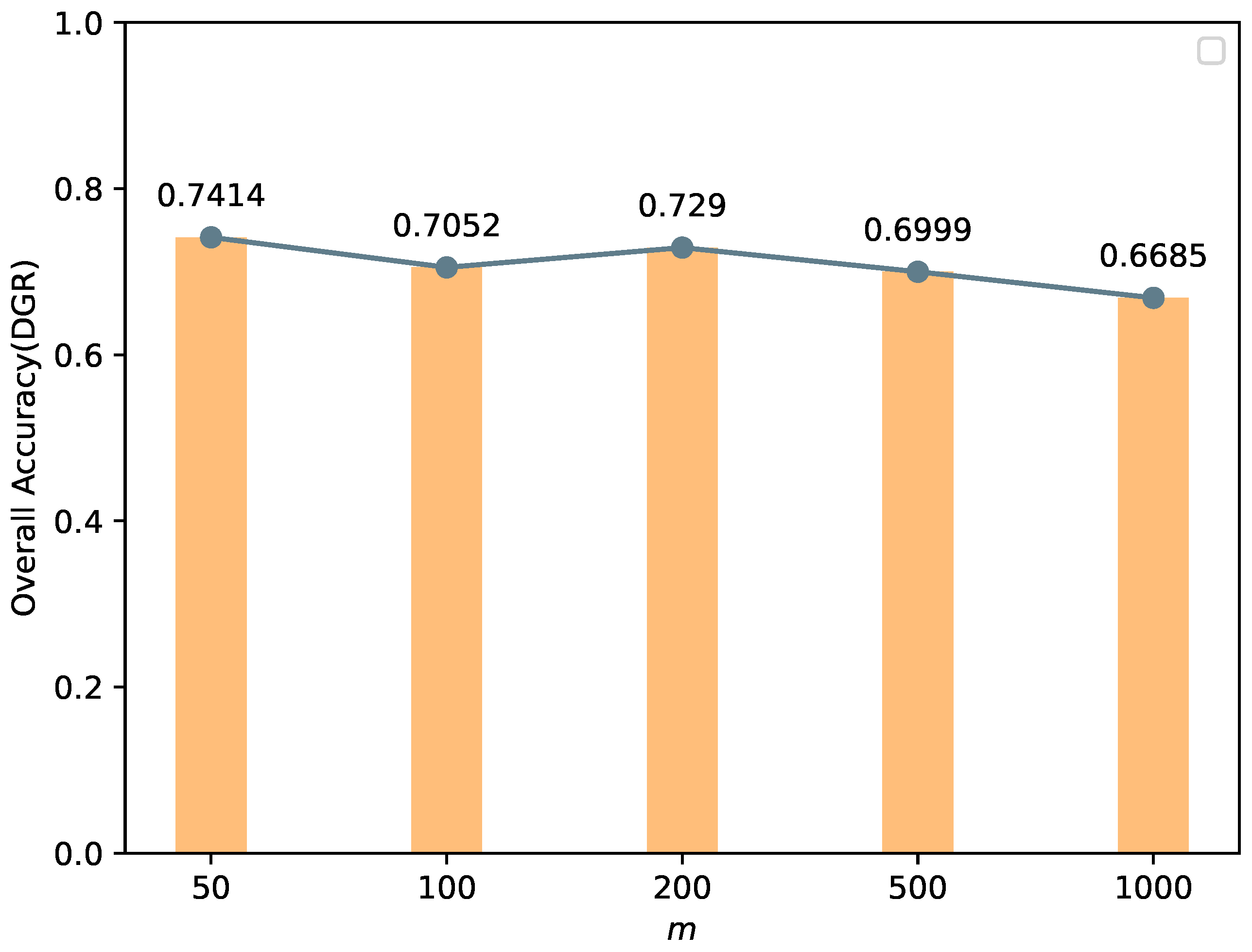
4.6. Sensitivity Analysis

Finally, we perform a sensitivity analysis. The two techniques of edge feature enhancement and selective replay used in the edge exemplar enhancement process proposed in this paper introduce different parameters, respectively. In the edge feature enhancement, the parameter $\eta$ is introduced as a penalty item to control the weight of the loss. The parameter $\gamma$ is introduced in selective replay to control the proportion of replayed edge exemplars. In this part of the experiment, we conduct a sensitivity analysis on these two parameters and set different values through grid search to observe their impact on model performance.

The first is the parameter $\gamma$. In the selective replay, the parameter $\gamma$ is used to control the proportion of replaying edge exemplars, $\gamma \in [0,1)$; and from the actual situation analysis, the proportion of edge samples should be smaller. In the sensitivity analysis in this part, we set different values of $\gamma$—respectively, 0.05, 0.1, 0.2, and 0.3—to verify the influence of parameter $\gamma$ on the model through experiments.

The result is shown in Figure 9. DGR-EE is more sensitive to $\gamma$. When $\gamma$ reaches 0.3, the model performance drops significantly. However, BI-R-EE is not sensitive to the parameter $\gamma$, and the recognition performance of the different $\gamma$ value models set in this paper has not changed significantly.

The second is the parameter $\eta$, which is the weight of the loss through the parameter $\eta$ as the penalty coefficient in the edge feature enhancement. In this part, we set different values of $\eta$, which are 0.01, 0.1, 0.5, 1.0, 5.0, 10.0, and 100.0. And the influence of the parameter $\eta$ on the model is verified through experiments.

The experimental results are shown in Figure 10. The dotted line in the figure indicates the lowest overall accuracy among the tested values. In BI-R-EE, when $\eta =100.0$, it reaches the lowest. At the same time, the overall accuracy shows a trend of rising first and then falling, which is also in line with expectations. When $\eta$ is small, the replay coefficient of edge samples is low. At this time, the penalty coefficient for edge samples being misclassified is low, and replay struggles to achieve the purpose of enhancing the memory of old edge samples in the model. When the penalty coefficient is too large, the edge samples will be. This affects the model’s cognition of the category, bringing a large intra-class bias, and the accuracy of the model will also decrease. The experimental results of DGR-EE are similar to those of BI-R-EE, but the optimal $\eta$ value is different, which also shows that the selection of $\eta$ needs to be adjusted according to the actual situation in the process of using edge exemplar enhancement.

In addition to the two hyperparameters used in the incremental learning model above, the edge exemplars size m defined in this paper is also an important parameter. In the sensitivity analysis of this section, we also set different values for m for comparative experiments, which are 50, 100, 200, 500, and 1000. The results of the experiment are shown in the Figure 11. We noticed a certain phenomenon in this experiment. When the value of m increased, especially when $m=1000$, the performance of the model dropped significantly, from 70%+ accuracy to 66%. We determined that the reason for this phenomenon is that a large m will causes edge exemplars to contain many non-edge samples. According to the results of the joint train, the classification accuracy can reach 94%, which means that there are fewer samples that will be misclassified in most categories, and there will be fewer forgotten edge samples. The selective replay adopted in this paper will further reduce the replay of edge examples, which will cause the model to forget the knowledge during the incremental learning process and reduce the identification accuracy.

4.7. Time and Space Complexity

The purpose of incremental learning is to continuously learn new knowledge from new tasks and to preserve the knowledge of previous tasks at a small cost of time and space. Therefore, time and space complexity analysis is an important indicator for the evaluation of an incremental learning model. In this section, we compare several types of incremental learning models based on the above experiments. The training time directly utilized the duration of the model training. And the space complexity is approximated by the stored model and data. Let $phi$ be the space used to store a classification model. We obtain the comparison results of the training time and storage space of these incremental learning models, as shown in

Table 8. Comparison of training time and storage space of different incremental learning models.

Model	Train Time (s)	Storage
LwF	580	$\varphi$
iCaRL	2005	$\varphi +K$
DGR	2090	$3\ast \varphi$
DGR-EE	2327	$3\ast \varphi +N\ast k$
BI-R	7253	$2\ast \varphi$
BI-R-EE	7579	$2\ast \varphi +N\ast k$

Note: The DGR contains three parts: the generator, the discriminator, and the classifier. Therefore, it needs to use $3\varphi$ space to store the model. The BI-R uses the replay-through-feedback technique to add a layer after the encoder as a classifier, so the BI-R model cost $2\varphi$. K is the exemplar set size of iCaRL; k is the number of edge exemplars for each class in this paper.

.

After utilizing edge exemplar enhancement, training time increased by 11.3% for DGR-EE and 4.5% for BI-R-EE. The increased training time comes from the construction of edge exemplars and the processing of selective replay. In practical applications, the increase in time consumption is far less than the training time of the model. From the perspective of space complexity, the increased space consumption is due to the storage of the edge exemplars set. And this storage space can be controlled. In this paper, the number of stored samples is set to 100. If there is storage pressure due to the increase in detection types, the number of stored samples can be appropriately reduced.

5. Discussion

Tor-obfuscated traffic detection using incremental learning models is a promising research direction. There are currently dozens of PTs, and many of them are being maintained and updated. When a supervised learning model is trained, it can only detect fixed types of obfuscated traffic. This limits the application of artificial intelligence to traffic detection. In highly adversarial scenarios such as intrusion detection and obfuscated traffic detection, the incremental learning model can meet the dynamic expansion requirements of the detection system. In the face of new detection requirements, there is no need to re-collect data and train models, and it also greatly reduces the storage requirements of the detection system for training data.

However, the application of the current incremental learning model still has great limitations. The first problem is analyzed in Section 3.1 of this article. The incremental learning model requires the same feature set extracted from all types of samples, which limits the application of many features, such as the front domain name in Meek, the protocol fingerprint of DTLS, etc. These features are often used for traffic detection, but Obfs4 does not contain them, so these features cannot be applied to incremental learning models. In this paper, we try to analyze the communication characteristics of some existing PTs and construct a flow statistical feature set from the transport layer to realize incremental learning of some PT traffic. This processing actually limits the recognition ability of the model. The second problem is the catastrophic forgetting problem of incremental learning. Although many methods have been proposed to alleviate the catastrophic forgetting of incremental learning models, we can still observe this phenomenon. In the experiment of this article, the fourth task start model has a 7% gap with the joint train, and this number will increase as the number of tasks increases.

After using the edge exemplar enhancement technique in this paper, the performance of the model changes in the two dimensions of intra-task and inter-task. In the experimental analysis of this paper, edge samples are replayed due to edge exemplar enhancement, and the influence of these samples on the model is enhanced through the parameter $\eta$. This also leads to a shift in the knowledge learned by the model on the previous task, resulting in an increase in the intra-task bias. However, it prevents the model from forgetting too much edge information and ensures the improvement of inter-task performance indicators so as to achieve the purpose of improving the overall performance of the model. The reduction in inter-task bias makes it possible to train some auxiliary models. Consider the following scenario. In Table 7, the recognition accuracy rate of the model after training is only 77% on the three categories of T2. We can consider using T2 data to train a three-category model during the training process. The incremental learning model is recognized as the data of the categories in T2 for secondary classification to improve identification accuracy.

The above discussion considered the potential influencing factors of the incremental learning model at the algorithm level. However, in pratical deployment, the model is also subject to serveral additional challenges. The first challenge is the bias of the dataset. In the dataset used in this article, we simulate the process of the continuous expansion of Tor detection needs by combining public datasets and self-collected data sets. However, in T3, the self-collected data are mainly web browsing and video traffic. This process will make the trained model more inclined to identify the traffic of web browsing and video. This may reduce the generalizability of the model. It is also a problem that many supervised learning models still exist. Few-shot learning or one-class learning models can help in the learning of specific patterns of samples on limited data to alleviate this problem. The second problem is the computational overhead problem of the actual deployment of the model. In the feature set designed in this article, we use features such as flow duration and average flow speed. These features need to be calculated after the flow ends. Therefore, the functional bottleneck of the framework proposed in this article lies in feature extraction. For small-scale detection, the use of the dpkt library in Python2.7 can realize traffic analysis. If the traffic scale is large, libnids can be used for flow reorganization and feature extraction. When the model is deployed for large-scale traffic detection, load balancing and multi-threaded parallelism can be used to ensure that the feature extraction module can extract features of large-scale traffic in real time. The load-balancing mechanism distributes flow data packets across multiple devices hosting the feature extraction module. Upon receiving a sufficient batch of packets, each feature extraction module initiates the statistical feature computation, which is then forwarded to the model detection module for analysis. Meanwhile, to ensure that the model detection module can process these data in a timely and effective manner, the GPU can be used to accelerate the model calculation. This process ensures reliable model deployment for large-scale traffic detection and recognition tasks. Finally, the challenge of online model updates must be addressed. During deployment, maintaining detection accuracy under evolving requirements becomes critical. Experimental results demonstrate a consistent decline in model accuracy as demands increase, with the performance gap compared to joint train widening significantly. To mitigate this, the model must strategically discard some previous task detection requirements to preserve accuracy. For instance, a threshold can be set, and the model needs to be retrained when the number of categories reaches the threshold.

Tor traffic detection based on incremental learning models is still a highly promising area of research. In this detection and obfuscation confrontation scenario, it is of great significance to reduce the re-training through incremental learning. However, in the online environment, the traffic of new PTs usually appears in the form of unknown traffic. This feature allows Tor traffic detection based on incremental learning to have an extended research direction. The first concerns unknown traffic discovery, that is, the open-world detection problem. Upon deployment, the model inevitably encounters unknown inputs, which are systematically misclassified into known categories due to the closed-set assumption. To address this issue, integrating open set recognition with incremental learning offers a viable solution. An N-class classifier is obtained after incremental learning. Then, the open set recognition model can be established based on the classifier, such as Openmax [28] or KLND [29]. It introduces an N + 1-dimensional output vector through extreme value theory. This output contains the probability of N known classes and the probability of an unknown class. This method enables the detection of unknown traffic patterns. Another important research work is the automatic discovery of new PTs. In the framework of this paper, it is assumed that new PTs are discovered manually and that their traffic can be actively collected. The discovery of unknown PT traffic is also a meaningful research area. For example, further analysis and discovery can be performed from the unknown traffic annotated by open set recognition. Anomaly detection and one-class learning models can also help discover unknown data. By clustering these unknown data, samples with similar features are aggregated together into clusters. Only a small number of samples in the cluster need to be manually analyzed to determine whether it is new PT traffic. This method enables the rapid analysis and discovery of new PTs.

6. Conclusions

Tor anonymous traffic obfuscation detection is a process of dynamic confrontation. Tor provides PTs to allow users and developers to freely choose traffic obfuscation methods. On the one hand, these PTs can disguise the features of Tor-obfuscated traffic and make it hard to detect by censors; on the other hand, PTs are also updating dynamically, such as from Obfs2 to Obfs4, and from Flashproxy to Snowflake. It requires censors to have continuous learning abilities. Therefore, this paper proposes an incremental learning framework with edge exemplar enhancement to detect Tor-obfuscated traffic. It proposes to build edge exemplars to enhance the incremental learning model through edge feature enhancement and selective replay. Finally, we combine public datasets and self-captured traffic from the Tor browser to simulate the application scenario. And the effectiveness of the edge exemplar enhancement proposed in this paper has been verified by experiments. The experimental results show that the accuracy of DGR-EE has increased by 21% compared to DGR. The accuracy of BI-R-EE has increased by 4% compared to BI-R.

Since deep learning is widely used in traffic detection, some researchers have begun to try to use the anti-machine learning method to construct obfuscated traffic. It will reduce the probability of its obfuscated traffic being detected by the deep learning model [30,31,32]. In summary, the detection of obfuscated traffic is still a challenging issue in Tor traffic detection. Although the incremental learning framework is proposed in this paper to enhance the confrontation ability of censors, it still requires manual analysis to construct detection features. It also cannot deal with AML-based traffic obfuscation. Therefore, it requires researchers to keep an eye on Tor-obfuscated traffic detection.

References

1. Reed, M.G.; Syverson, P.F.; Goldschlag, D.M. Anonymous connections and onion routing. IEEE J. Sel. Areas Commun. 1998, 16, 482–494. [Google Scholar] [CrossRef]
2. Zantout, B.; Haraty, R.A. I2P data communication syste. In Proceedings of the ICN 2011: The Tenth International Conference on Networks, St. Maarten, The Netherlands, 23–28 January 2011; pp. 401–409. [Google Scholar]
3. Clarke, I.; Sandberg, O.; Wiley, B.; Hong, T.W. Freenet: A distributed anonymous information storage and retrieval system. In Designing Privacy Enhancing Technologies: International Workshop on Design Issues in Anonymity and Unobservability Berkeley; Springer: Berlin/Heidelberg, Germany, 2001. [Google Scholar]
4. Wang, L.; Mei, H.; Sheng, V.S. Multilevel identification and classification analysis of Tor on mobile and PC platforms. IEEE Trans. Ind. Inform. 2021, 17, 1079–1088. [Google Scholar] [CrossRef]
5. Gurunarayanan, A.; Agrawal, A.; Bhatia, A.; Vishwakarma, D.K. Improving the performance of Machine Learning Algorithms for TOR detection. In Proceedings of the 2021 International Conference on Information Networking (ICOIN), Jeju Island, Republic of Korea, 13–16 January 2021; pp. 439–444. [Google Scholar]
6. Rao, Z.; Niu, W.; Zhang, X.; Li, H. Tor anonymous traffic identification based on gravitational clustering. Peer-Peer Netw. Appl. 2018, 11, 592–601. [Google Scholar] [CrossRef]
7. Yao, Z.; Ge, J.; Wu, Y.; Zhang, X.; Li, Q.; Zhang, L.; Zou, Z. Meek-based tor traffic identification with hidden markov model. In Proceedings of the 2018 IEEE 20th International Conference on High Performance Computing and Communications; IEEE 16th International Conference on Smart City; IEEE 4th International Conference on Data Science and Systems (HPCC/SmartCity/DSS), Exeter, UK, 28–30 June 2018; pp. 335–340. [Google Scholar]
8. Soleimani, M.H.; Mansoorizadeh, M.; Nassiri, M. Real-time identification of three Tor pluggable transports using machine learning techniques. J. Supercomput. 2018, 74, 4910–4927. [Google Scholar] [CrossRef]
9. He, Y.; Hu, L.; Gao, R. Detection of tor traffic hiding under obfs4 protocol based on two-level filtering. In Proceedings of the 2019 2nd International Conference on Data Intelligence and Security (ICDIS), South Padre Island, TX, USA, 28–30 June 2019; pp. 195–200. [Google Scholar]
10. Hu, Y.; Zou, F.; Li, L.; Yi, P. Traffic classification of user behaviors in tor, i2p, zeronet, freenet. In Proceedings of the 2020 IEEE 19th International Conference on Trust, Security and Privacy in Computing and Communications (TrustCom), Guangzhou, China, 29 December 2020–1 January 2021; pp. 418–424. [Google Scholar]
11. Salman, O.; Elhajj, I.H.; Kayssi, A.; Chehab, A. Denoising adversarial autoencoder for obfuscated traffic detection and recovery. In Machine Learning for Networking, Proceedings of the Second IFIP TC 6 International Conference, Paris, France, 3–5 December 2019; Springer: Cham, Switzerland, 2020; pp. 99–116. [Google Scholar]
12. Xu, W.; Zou, F. Obfuscated Tor Traffic Identification Based on Sliding Window. Secur. Commun. Netw. 2021, 2021, 5587837. [Google Scholar] [CrossRef]
13. Lin, K.; Xu, X.; Gao, H. TSCRNN: A novel classification scheme of encrypted traffic based on flow spatiotemporal features for efficient management of IIoT. Comput. Netw. 2021, 190, 107974. [Google Scholar] [CrossRef]
14. Chen, J.; Cheng, G.; Mei, H. F-ACCUMUL: A Protocol Fingerprint and Accumulative Payload Length Sample-Based Tor-Snowflake Traffic-Identifying Framework. Appl. Sci. 2023, 13, 622. [Google Scholar] [CrossRef]
15. Li, Z.; Wang, M.; Wang, X.; Shi, J.; Zou, K.; Su, M. Identification Domain Fronting Traffic for Revealing Obfuscated C2 Communications. In Proceedings of the 2021 IEEE Sixth International Conference on Data Science in Cyberspace (DSC), Shenzhen, China, 9–11 October 2021; pp. 91–98. [Google Scholar]
16. Lashkari, A.H.; Gil, G.D.; Mamun, M.S.; Ghorbani, A.A. Characterization of tor traffic using time based features. In Proceedings of the 3rd International Conference on Information Systems Security and Privacy, Porto, Portugal, 19–21 February 2017; pp. 253–262. [Google Scholar]
17. Shapira, T.; Shavitt, Y. Flowpic: Encrypted internet traffic classification is as easy as image recognition. In Proceedings of the IEEE INFOCOM 2019—IEEE Conference on Computer Communications Workshops (INFOCOM WKSHPS), Paris, France, 29 April–2 May 2019; pp. 680–687. [Google Scholar]
18. Shapira, T.; Shavitt, Y. FlowPic: A generic representation for encrypted traffic classification and applications identification. IEEE Trans. Netw. Serv. Manag. 2021, 18, 1218–1232. [Google Scholar] [CrossRef]
19. van de Ven, G.M.; Tuytelaars, T.; Tolias, A.S. Three types of incremental learning. Nat. Mach. Intell. 2022, 4, 1185–1197. [Google Scholar] [CrossRef] [PubMed]
20. Li, Z.; Hoiem, D. Learning without forgetting. IEEE Trans. Pattern Anal. Mach. Intell. 2017, 40, 2935–2947. [Google Scholar] [CrossRef] [PubMed]
21. Rebuffi, S.A.; Kolesnikov, A.; Sperl, G.; Lampert, C.H. icarl: Incremental classifier and representation learning. In Proceedings of the IEEE conference on Computer Vision and Pattern Recognition, Honolulu, HI, USA, 21–26 July 2017; pp. 2001–2010. [Google Scholar]
22. Shin, H.; Lee, J.K.; Kim, J.; Kim, J. Continual learning with deep generative replay. In Proceedings of the 31st International Conference on Neural Information Processing Systems, Long Beach, CA, USA, 4–9 December 2017. [Google Scholar]
23. Van de Ven, G.M.; Siegelmann, H.T.; Tolias, A.S. Brain-inspired replay for continual learning with artificial neural networks. Nat. Commun. 2020, 11, 4069. [Google Scholar] [CrossRef] [PubMed]
24. Kingma, D.P.; Ba, J. Adam: A method for stochastic optimization. arXiv 2014, arXiv:1412.6980. [Google Scholar]
25. Gulrajani, I.; Ahmed, F.; Arjovsky, M.; Dumoulin, V.; Courville, A.C. Improved training of wasserstein gans. In Proceedings of the 31st International Conference on Neural Information Processing Systems, Long Beach, CA, USA, 4–9 December 2017. [Google Scholar]
26. Kingma, D.P.; Welling, M. Auto-encoding variational bayes. arXiv 2013, arXiv:1312.6114. [Google Scholar]
27. Emanuele, P.; Giuseppe, L.; Claudio, C.; Leonardo, Q. Peel the onion: Recognition of android apps behind the tor network. In Proceedings of the 15th Information Security Practice and Experience, ISPEC 2019, Kuala Lumpur, Malaysia, 26–28 November 2019; pp. 95–112. [Google Scholar]
28. Bendale, A.; Boult, T.E. Towards open set deep networks. In Proceedings of the IEEE Conference on Computer Vision and Pattern Recognition, Las Vegas, NV, USA, 27–30 June 2016; pp. 1563–1572. [Google Scholar]
29. Dahanayaka, T.; Ginige, Y.; Huang, Y.; Jourjon, G. Robust open-set classification for encrypted traffic fingerprinting. Comput. Netw. 2016, 236, 109991. [Google Scholar] [CrossRef]
30. Yang, F.; Wen, B.; Comaniciu, C.; Subbalakshmi, K.P.; Chandramouli, R. TONet: A Fast and Efficient Method for Traffic Obfuscation Using Adversarial Machine Learning. IEEE Commun. Lett. 2022, 26, 2537–2541. [Google Scholar] [CrossRef]
31. Liu, L.; Yu, H.; Yu, S.; Yu, X. Network Traffic Obfuscation against Traffic Classification. Secur. Commun. Netw. 2022. [Google Scholar] [CrossRef]
32. Liu, H.; Dani, J.; Yu, H.; Sun, W.; Wang, B. Advtraffic: Obfuscating encrypted traffic with adversarial examples. In Proceedings of the 2022 IEEE/ACM 30th International Symposium on Quality of Service (IWQoS), Oslo, Norway, 10–12 June 2022; pp. 1–10. [Google Scholar]
Figure 1. Summarized hierarchy of Tor traffic identification.
Electronics 14 01589 g001
Figure 2. The working principle of three built-in pluggable transmissions in Tor browser: Obfs4, Meek and Snowflake.
Electronics 14 01589 g002
Figure 3. Incremental learning framework of Tor obfuscated traffic.
Electronics 14 01589 g003
Figure 4. The network structure and replay process of edge exemplars enhancement in incremental learning.
Electronics 14 01589 g004
Figure 5. The network struct of AAE.
Electronics 14 01589 g005
Figure 6. The model is shown for different evaluation metrics: (a) the recognition accuracy of the model on each category; (b) the overall recognition accuracy of different models; (c) the variation of the test accuracy of different models during the incremental learning process.
Electronics 14 01589 g006
Figure 7. The task confusion matrix of different models: (a) DGR; (b) DGR-EE; (c) BI-R; (d) BI-R-EE.
Electronics 14 01589 g007
Figure 8. Ablation experiment results. The model evaluation metrics of edge feature enhancement and selective replay on BI-R.
Electronics 14 01589 g008
Figure 9. The sensitivity analysis result of the model to the proportion of replayed samples ( γ ).
Electronics 14 01589 g009
Figure 10. The sensitivity analysis result of the edge feature enhancement loss weight η .
Electronics 14 01589 g010
Figure 11. The sensitivity analysis result of the edge exemplars size (m).
Electronics 14 01589 g011