DyLKANet: A Lightweight Dynamic Distillation Network for Remote Sensing Image Super-Resolution Based on Large-Kernel Attention

Abstract

Lightweight remote sensing image super-resolution methods aim to enhance image resolution and recover fine details through lightweight neural networks. However, current lightweight methods still suffer from poor performance and unattractive details. DyLKANet introduces a novel lightweight architecture that utilizes a multi-level feature integration strategy to enhance information exchange between context-aware and large kernel attention mechanisms. The network comprises two core modules: the feature distillation and enhancement block for efficient feature extraction, and the context-aware attention-based feature fusion module for capturing global interdependencies. Experiments conducted on the UCMerced, AID, and DIV2K datasets reveal that DyLKANet achieves comparable performance while maintaining a low parameter count and computational complexity. Taking the 2× upscaling results on the UCMerced dataset as an example, specifically, DyLKANet improves PSNR by 0.212–3.544 dB, SSIM by 0.005–0.038, and reduces parameters by 18.79–95.46%. DyLKANet reduces FLops by 7.25–82.63%, making it a promising solution for remote sensing image super-resolution tasks in resource-constrained environments.

1. Introduction

High-resolution remote sensing images are extensively utilized in ecological monitoring, crop assessment, urban planning, military reconnaissance, and disaster response due to their wide coverage, rich information, and enduring records [1]. However, the undersampling effect of imaging sensors and various degradation factors in the imaging process significantly limit the acquisition of high-resolution remote sensing images. Enhancing resolution through improved hardware performance involves significant costs and risks. Therefore, achieving high-resolution images without hardware modifications is crucial for remote sensor design, improving human visual perception, and advancing subsequent applications.

Single-image super-resolution (SISR) is a fundamental challenging task in computer vision, focusing on reconstructing low-resolution images into high-resolution ones by recovering high-frequency details lost due to imaging system limitations [2]. The evolution of SISR techniques has gradually transitioned from the initial simple interpolation methods such as neighborhood interpolation, bi-quadratic interpolation, and bi-tertiary interpolation, to the degradation process of considering SISR as a difficult problem to solve and inversely solving it by mathematical modeling of image sampling [3]. This technology has demonstrated wide application potential in various fields such as remote sensing and medical imaging [4], and can effectively improve the processing quality and effectiveness of subsequent related tasks [5]. Numerous variants of Convolutional Neural Networks (CNNs) and Visual Transformers (ViTs) have been developed to model the nonlinear relationship between low-resolution (LR) and high-resolution (HR) image pairs. Early CNN-based models, including SRCNN [6], SCN [7], and FSRCNN [8], prioritized simplicity but struggled to preserve high-frequency details. The development of deep residual networks (e.g., VDSR [9], LapSRN [10], EDSR [11]), and recurrent neural networks (e.g., DRCN [12], DRRN [13]) enabled multi-scale super-resolution reconstruction. Additionally, advanced architectures such as densely connected networks (e.g., SRDenseNet [14], RDN [15]), generative adversarial networks (e.g., SRGAN [16], RFB-ESRGAN [17]), and attention-based networks (e.g., SAN [18]) have significantly improved super-resolution performance at high magnifications. These innovations enhance reconstruction quality and introduce novel neural network structures, including SRFormer [19], CROSS-MPI [20], SRWARP [21], IMDN [22], ECBSR [23], and FMEN [24]. Recently, Transformer architectures have gained prominence in SISR due to their self-attention mechanisms, which capture global information and leverage image self-similarity. Models like TTSR [25], ESRT [26], SwinIR [27], and TransENet [28] improve global dependency handling by employing techniques such as feature dimension fusion, cross-token attention, and sliding windows. Despite the progress of CNN- and Transformer-based methods in SISR, their high parameter counts and computational complexity pose significant challenges, particularly for resource-constrained devices. Thus, further research is needed to optimize the balance among performance, parameter count, and computational complexity.

Remote sensing images exhibit diverse feature types and are affected by multiple degradation factors, including sampling errors, shape distortions, sharpness loss, and noise interference during imaging. Additionally, ground artifacts caused by lighting changes, such as cloud cover, terrain variations, and haze, further increase their semantic complexity compared to natural images, complicating remote sensing image super-resolution (RSISR). Researchers have introduced methods such as the characteristic resonance loss function [29], a two-stage design strategy incorporating spatial and spectral knowledge [30], and a hybrid higher-order attention mechanism [31] to address these challenges. However, these approaches still struggle with the complexities inherent in natural image super-resolution networks. Thus, there is an urgent need for lightweight RSISR techniques capable of efficiently processing massive remote-sensing images.

Recently, many lightweight super-resolution models have been developed, employing techniques such as cascading mechanisms [32], special convolutional layers [33], context-switching layers [34], channel-separation strategies [35], multi-feature distillation [22], neighborhood filtering [36], hierarchical feature fusion [37,38,39], novel self-attention mechanisms [40,41,42], large kernel distillation [43,44], and N-Gram contextual information [45]. CNN-based methods reduce model parameters by decreasing convolutional layers or residual blocks [46] and using dilated or group convolutions instead of traditional operations, often employing recursive structures or parameter-sharing strategies [12,13,38]. Transformer-based methods reduce computational complexity using small windows and sliding mechanisms. However, most of these models are limited to capturing local or regional interdependencies and struggle to explicitly capture long-range global dependencies across the entire image. This limitation is primarily due to the high computational cost of capturing global dependencies. Therefore, existing lightweight RSISR methods require further optimization and breakthroughs to enhance performance.

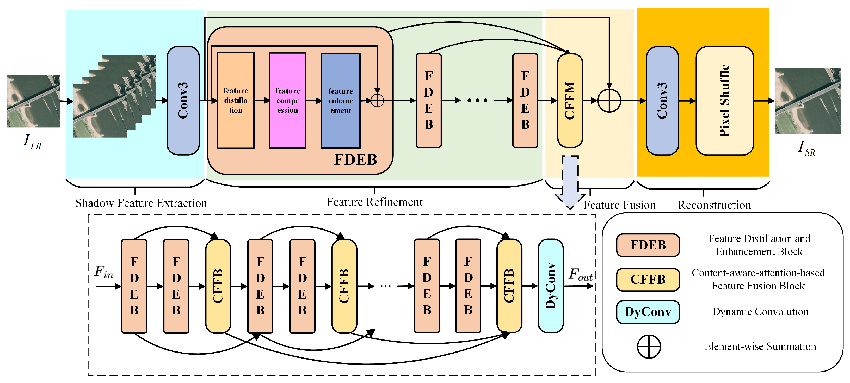
This paper introduces a super-resolution reconstruction method for remote sensing images, employing a dynamic large kernel attention-based feature distillation and fusion network (DyLKANet) to overcome the limitations of existing RSISR methods. The DyLKANet employs a multi-level feature integration strategy to facilitate information exchange between the context-aware attention mechanism and the large kernel attention mechanism. The DyLKANet framework comprises two key modules: the feature distillation and enhancement block (FDEB) for efficient feature extraction, and the context-aware attention-based feature fusion module (CFFM) for capturing global interdependencies. The primary contributions of this study are outlined as follows:

(1)

DyLKANet introduces a novel lightweight network architecture that employs a multi-level feature integration strategy. This strategy facilitates information exchange between the context-aware attention mechanism and the large kernel attention mechanism, enhancing the overall performance of the network;

(2)

We designed a dynamic convolutional residual block, which utilizes dynamic convolution to adaptively generate convolution kernels for each input sample. This approach not only reduces computational overhead but also preserves the depth of feature extraction;

(3)

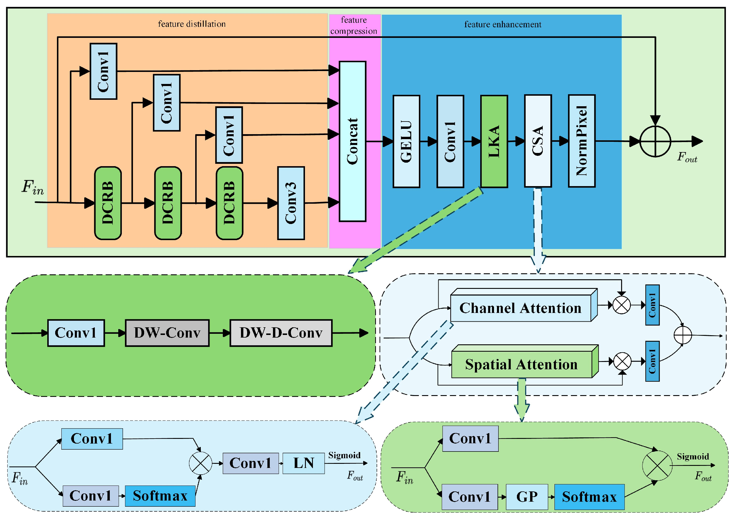
The proposed feature distillation and enhancement block incorporates feature distillation, compression, and enhancement stages. This block is capable of efficiently extracting key features while significantly reducing the number of parameters, contributing to the lightweight nature of DyLKANet.

The rest of the paper is organized as follows. Section 2 is the description of the methodology proposed in this paper. Section 3 analyzes the experiments and results. Section 4 analyzes and discusses the validity of each component of the proposed method and Section 5 gives a conclusion.

2. Methods

This section describes the architecture of the proposed dynamic distillation and fusion lightweight network, termed DyLKANet, which utilizes large-kernel attention and dynamic convolution. Next, the feature distillation and enhancement block (FDEB) and dynamic convolutional residual block (DCRB) are then described in detail. Finally, the context-aware-attention-based feature fusion block (CFFB) is introduced.

2.1. Network Architecture

As shown in Figure 1, the proposed DyLKANet architecture includes four stages: shallow feature extraction, deep feature refinement, multi-layer feature fusion, and super-resolution image reconstruction from the LR input. $I_{LR}$ and $I_{SR}$ represent the input and output images, respectively. Before shallow feature extraction, the input image is duplicated $n$ times and merged along the channel dimensions, increasing the available image information. Subsequently, shallow feature extraction is performed using a standard 3 × 3 convolution. This process is represented as follows.

$$F_0=H_{Conv3\times 3}\left(I_{LR}^1,\cdots ,I_{LR}^m\right)$$

(1)

where $H_{Conv3\times 3}$ is the convolution operation and $F_0$ is the extracted shallow features. $F_0$ is then used as input to the deep feature refinement layer. The deep feature refinement layer is composed of $n$ FDEBs.

$$\begin{array}{c}{F}_1=H_{FDEB}^1\left(F_0\right)\\ \cdots \\ F_n=H_{FDEB}^n\left(F_{n-1}\right)\end{array}$$

(2)

where $H_{FDEB}^i$ is the i-th FDEB and $F_n$ is the extracted feature information. $F_1\cdots F_n$ will then be used as the input to the feature fusion layer CFFM. The Content-aware-based Multi-scale Feature Fusion Module (CFFM) is a module composed of FDEBs and CFFBs, with the structure being recursively called.

$$\begin{array}{c}{F}_{in}^0=C_s\left(F_1,\cdots F_n\right)\\ F_j^1=H_{FDEB}\left(F_{in}^{j-1}\right)\\ F_j^2=H_{FDEB}\left(F_j^1\right)\\ O_j=H_{CFFB}\left(C_s\left(F_j^{2i-2},F_j^{2i}\right)\right)\\ C_f=H_{CFFB}\left(O_1,\dots ,O_6\right)\end{array}$$

(3)

where $C_s$ denotes the stacking operation. $F_j^1$ and $F_j^2$ represent the FDEB results in the $j$th recursively called structure, $C_f$ is the condensed feature, while $O_j$ denotes the CFFB results in the same structure. $j$ denotes the number of recursively calls to the structure. Except for the first call where $F_{in}^{j-1}=F_{in}^0$, every subsequent call sets $F_{in}^{j-1}=C_s\left(F_j^1,O_j\right)$. The final recursive call requires the output of the CFFM structure from preceding iterations into the last CFFM. The final $O_j$ from the recursive calls is processed by dynamic convolution (DyConv) to perform feature fusion. Finally, the output $F_{out}$ from the fusion layer, along with $F_0$, is input into the SR image reconstruction layer.

$$F_{out}=DyConv\left(C_f\right)$$

(4)

The reconstruction layer includes a 3 × 3 convolution and a sub-pixel convolution applied to the $F_0$ and $F_{out}$ features. The process of up-sampling can be formulated as:

$$I_{SR}=Rec\left(F_{out}+F_0\right)$$

(5)

where $Rec$ is the image reconstruction operation, and $I_{SR}$ is the generated SR image.

2.2. Feature Distillation and Enhancement Block

Receptive field diversity is essential for capturing contextual information, particularly in reconstructing remotely sensed images. Based on the principle of feature distillation, we introduce the FDEB, as illustrated in Figure 2.

The FDEB comprises three phases: feature distillation, feature compression, and feature enhancement. The distillation phase employs the DCRB module to reduce parameters and uses additional convolutional layers to refine input features and extract key features progressively. The distillation phase reduces the number of feature channels by half, thereby selectively extracting key features. This can be expressed as follows:

$$\left\{\begin{array}{c}{F}_1^{rough}=H_{DCRB}\left(F_{in}\right)\\ F_2^{rough}=H_{DCRB}\left(F_1^{rough}\right)\\ F_3^{rough}=H_{DCRB}\left(F_2^{rough}\right)\\ F_4=Con{v}_3\left(F_3^{rough}\right)\\ F_1^{distill1}=Con{v}_1\left(F_{in}\right)\\ F_2^{distill2}=Con{v}_1\left(F_1^{rough}\right)\\ F_3^{distill3}=Con{v}_1\left(F_2^{rough}\right)\end{array}\right.$$

(6)

where $F_n^{rough}$ and $F_n^{distilln}$ represent the n-th coarse and refined features, respectively. $H_{DCRB}$, defined as the dynamic convolution operation applied to residual blocks, handles the refinement process to enhance feature representation. Additionally, $Con{v}_1$ and $Con{v}_3$ manage the distillation process, emphasizing the extraction of key features.

In the feature compression stage, the features extracted from different layers are concatenated and then processed through a 1 × 1 convolutional layer to synthesize the fused features, which can be expressed as follows:

$$F_{fusion}=Con{v}_1\left(Concat\left(F_1^{distill1},F_2^{distill2},F_3^{distill3},F_4\right)\right)$$

(7)

where $F_{fusion}$ denotes the fused feature.

In the feature enhancement stage, large kernel attention (LKA) is cascaded with Channel and Spatial Attention (CSA) to enhance feature representation. Applying CSA following LKA enables further feature fusion and refinement. While LKA captures macroscopic features, CSA refines these features, resulting in more precise and targeted fusion. This process is expressed as follows:

$$H_{LKA}=Con{v}_{1\times 1}\left(Con{v}_{DWD}\left(Con{v}_{DW}\left(F_{fusion}\right)\right)\right)$$

(8)

$$\begin{array}{c}{H}_{CSA}=B^{CA}\oplus B^{SA}\\ B^{CA}=Con{v}_{1\times 1}\left(Softmax\left(Con{v}_{1\times 1}\left(F_{fusion}\right)\right)\otimes Con{v}_{1\times 1}(F_{fusion}\right))\\ B^{SA}=Con{v}_{1\times 1}\left(Softmax\left(GP\left(Con{v}_{1\times 1}\left(F_{fusion}\right)\right)\right)\otimes Con{v}_{1\times 1}\left(F_{fusion}\right)\right)\end{array}$$

(9)

$$F_e=H_{CSA}(H_{LKA}\left(F_{fusion}\right))$$

(10)

where $H_{LKA}$ is the operation employing LKA, $H_{CSA}$ is the operation utilizing CSA, $B^{CA}$ is the channel attention branch, $B^{SA}$ is the spatial attention branch, and $F_e$ is the enhanced feature. To enhance model performance, a pixel normalization module is incorporated during the feature transformation stage to stabilize model training.

$$F_t=N_{pix}\left(H_{trans}\left(F_e\right)\right)$$

(11)

where $H_{trans}$ is the 1 × 1 convolutional operation, $N_{pix}$ is the pixel normalization operation, and $F_t$ is the transformed features. Finally, longer skip connections are used to enhance the residual learning capability of the model:

$$C_{out}=F_{trans}+F_{in}$$

(12)

2.3. Dynamic Convolutional Residual Block

To dynamically generate a specific convolution kernel for each input sample, the kernel is adaptively adjusted based on the features, offering an efficient strategy to reduce computational overhead while preserving feature extraction depth. We designed DyConv as a lightweight alternative to convolutional operations. We constructed DCRB (as shown in Figure 3) by combining DyConv with the depth-wise separable convolution DWConv and the GLUE activation function. In DCRB, DyConv dynamically generates convolution kernels, unlike traditional convolution, which operates on the entire channel set. The dynamic convolution kernel is denoted as:

$$\begin{array}{c}{K}_{Dynamic}={\displaystyle {\displaystyle \sum }_{i=1}^n}{w}_i·k_i^{dy}\\ D_0=H_{DyConv}\left(C_{in},K_{dynamic}\right)\end{array}$$

(13)

where $D_0$ represents the output after the DyConv, $C_{in}$ represents the input feature, $K_{Dynamic}$ is the convolution kernel, $w_i$ is the weight coefficients, and $k_i^{dy}$ is a candidate convolution kernel of the same dimension. Compared with traditional convolution, DyConv significantly reduces computational requirements. Next, DCRB utilizes depth-wise convolution (DWConv) to process the output $D_0$, generating intermediate results $D_{dw}$:

$$D_{fuse}=H_{BN}\left(H_{DWConv}\left(P_0\right)\right)$$

(14)

where $D_{fuse}$ represents the output after the DWConv, $H_{DWConv}$ represents the DWConv, $H_{BN}$ represents the BatchNorm, this step ensures that the depth of the network is not affected. Finally, by summing the input $C_{in}$ and fusion output $D_{fuse}$ and applying the GELU activation function, the final output $C_{out}$ of DCRB is obtained:

$$C_{out}=GELU\left(C_{in}+D_{fuse}\right)$$

(15)

where $C_{out}$ represents the output after the DCRB.

2.4. Context-Aware-Attention-Based Feature Fusion Block

In remote sensing image SR, utilizing hierarchical information is essential. To address this, we developed CFFM (as shown in Figure 1), which integrates features at different levels, capturing both low-level details and high-level semantics for improved representation. The core of the feature fusion architecture is the context-aware, attention-based feature fusion block (CFFB), shown in Figure 4.

The process begins with a series of $n$ input features, each containing $C$ channels. This can be expressed as follows:

$$\begin{array}{c}{F}_{concat}=Concat\left(F_1,F_2,F_3\right)\\ F_{refined}=Con{v}_1\left(F_{concat}\right)\\ F_i=H_{CAA}\left(F_{refined}\right)\end{array}$$

(16)

where $F_i$ is the feature of the i-th input. Then, dimensionality reduction is performed by a 1 × 1 convolutional operation. $F_{refined}$ is the refined feature that reduces the channel dimension back to $C$, retaining the most salient features. $F_{refined}$ is augmented by a context-aware attention mechanism (CAA).

Figure 4 illustrates the structure of the CAA. A set of feature maps is first passed through an average pooling layer, and the resulting sum is then processed by a convolutional layer (denoted as $Con{v}_1$) to augment the features. These features are subsequently approximated using two depth-wise convolutions. A sigmoid function is applied to generate combination coefficients, which range from 0 to 1. Finally, the input feature maps are multiplied by these coefficients to produce the output feature maps.

2.5. Training Losses

The objectives of network training are as follows: (1) to generate high-quality $I_{SR}$ through training; (2) to preserve $I_{LR}$ spatial structure and semantic information; (3) to uncover more detailed texture information in remote sensing images. In this paper, reconstruction loss, content loss, and total variation loss are used to train the network. The overall loss can be described as follows:

$$L_{total}={\lambda }_{rec}{L}_{rec}+{\lambda }_{content}{L}_{content}+{\lambda }_{TV}{L}_{TV}$$

(17)

The reconstruction loss is used to ensure the similarity between the generated image and the original image; thus, it is usually set ${\lambda }_{rec}$ to 1 or greater to avoid generating blurry images. Since L1 loss converges more easily than L2 loss, L1 loss is chosen as the reconstruction loss.

$$L_{rec}={\displaystyle \frac{1}{CHW}}{\left|\left|I_{HR}-I_{SR}\right|\right|}_1$$

(18)

For the complex textures and structural variations in remote sensing images, this paper chooses Huber loss as the content loss, because Huber loss can reduce generated artifacts when dealing with remote sensing images that have high noise and low resolution.

$$L_{content}=\left\{\begin{array}{c}{\displaystyle \frac{1}{2}}{\left(I_{HR}-I_{SR}\right)}^2, if \left|I_{HR}-I_{SR}\right|\le \delta \\ \delta (\left|I_{HR}-I_{SR}\right|-{\displaystyle \frac{1}{2}}\delta ), if \left|I_{HR}-I_{SR}\right|>\delta \end{array}\right.$$

(19)

where $I_{HR}$ denotes the true value, $I_{SR}$ denotes the predicted value, and $\delta$ is the threshold parameter.

The total variational loss $L_{TV}$ drives the resulting image to be smoother in smooth regions while preserving the sharpness of the edges.

$$\begin{array}{c}diff=I_{HR}-I_{SR}\\ L_{TV}={\displaystyle {\displaystyle \sum }_{i,j}}\sqrt{{\left(dif{f}_{i,j-1}-dif{f}_{i,j}\right)}^2+{\left(dif{f}_{i+1,j}-dif{f}_{i,j}\right)}^2}\end{array}$$

(20)

where $dif{f}_{i,j}$ is the pixel value of the $diff$ image at position (i,j).

3. Experiments and Results

This section outlines the implementation details, including datasets, evaluation metrics, experimental configurations, and training strategies. Comparative experiments are conducted on the UCMerced [47] and AID [48] datasets to analyze quantitative results and visualize them in comparison with state-of-the-art methods. Finally, the efficiency of the baseline model is evaluated against the proposed model using the UCMerced dataset.

3.1. Datasets

Two publicly available remote sensing datasets, UCMerced and AID, are used to validate the proposed model’s effectiveness. The UCMerced dataset contains 2100 images across 21 remote sensing scenes, with each category comprising 100 images of 256 × 256 pixels. The AID dataset consists of 10,000 images from 30 remote sensing scenes, including airports, farmland, beaches, and deserts, with each image of 600 × 600 pixels. Each dataset is divided into training, testing, and validation sets with an 8:1:1 ratio. During experiments, the original HR images from each dataset were used, while LR images were generated using bicubic interpolation to create HR-LR image pairs.

3.2. Metrics

The results were evaluated using the Peak Signal-to-Noise Ratio (PSNR) and Structural Similarity Index (SSIM).

$$PSNR\left(I_{HR},I_{SR}\right)=10log{\displaystyle \frac{{255}^2}{MSE\left(I_{HR},I_{SR}\right)}}$$

(21)

where

$$MSE\left(I_{HR},I_{SR}\right)={\displaystyle \frac{{\sum }_{W=1}^W{\sum }_{h=1}^H{\left(I_{HR}\left(h,w\right)-I_{SR}\left(h,w\right)\right)}^2}{H\times W}}$$

(22)

where $W$ and $H$ are the width and height of the image, respectively; the larger the PSNR value, the better the reconstruction effect.

$$SSIM\left(I_{HR},I_{SR}\right)={\displaystyle \frac{\left(2{\mu }_{I_{HR}}{\mu }_{I_{SR}}+C_1\right)\left({\sigma }_{I_{HR}{I}_{SR}}+C_2\right)}{\left({\mu }_{I_{HR}}^2+{\mu }_{I_{SR}}^2\right)\left({\sigma }_{I_{HR}}^2+{\sigma }_{I_{SR}}^2+C_2\right)}}$$

(23)

$SSIM\left(·\right)$ indicates the similarity between the HR image and the reconstructed SR image in terms of brightness, contrast, and structure. Larger SSIM values indicate higher image quality.

3.3. Experimental Settings

To ensure a fair comparison, a unified degradation model was used to generate the experimental dataset, and consistent data enhancement techniques were applied during model training. Six SISR methods—SRCNN, FSRCNN, IMDN, ECBSR FMEN, and OMNISR—and six RSISR methods—CTNet, FENet, HSENET, AMFFN, TransENet, TTST—were selected for this study. The proposed model was developed in this experimental environment using the PyTorch 1.12.0 framework on the Ubuntu 22.04 operating system. An NVIDIA RTX3090, manufactured by ASUS in Taipei, Taiwan, was used to accelerate model training. The GPU was manufactured by ASUS in Santa Clara, California, USA. During model training, the Adam optimizer was employed with momentum parameters ${\beta }_1$ = 0.9 and ${\beta }_2$ = 0.99. The batch size was set to 16. The initial learning rate was 0.0005, and a linear decay strategy was applied to adjust it progressively during the training cycle. Additionally, the performance of all models was evaluated at scales of ×2, ×3, and ×4. To emphasize details more strongly, we set the ${\lambda }_{rec}$, ${\lambda }_{content}$, and ${\lambda }_{TV}$ to 1, 1 × 10⁻¹, and 1 × 10⁻², respectively. The reconstruction loss is the only loss involved in the first three stages of the training process, while the content loss and total variation loss are added in the subsequent stages, up to the final stage.

3.4. Results of Experiments on UCMerced Dataset

Table 1. PSNR and SSIM results of the UCMerced test dataset for ×2, ×3, ×4.

Model	Year	Scale	Params [K]	FLops [G]	Memory [MB]	Time [ms]	UCMerced
							PSNR	SSIM
SRCNN	2014	×2	69	7.1	22	0.187	31.096	0.893
FSRCNN	2016	×2	25	6.7	134	0.407	33.148	0.914
IMDN	2019	×2	694	70.7	70	5.536	34.051	0.921
ECBSR	2021	×2	1387	139.9	252	10.053	34.061	0.922
OMNISR	2023	×2	772	77.6	686	16.031	34.201	0.925
FMEN	2022	×2	325	33.2	32	2.413	34.063	0.922
CTNet	2021	×2	349	26.2	252	8.509	34.066	0.922
FENet	2022	×2	351	34.3	468	94.258	34.125	0.922
HSENET	2022	×2	5290	16.7	1816	7.352	34.221	0.926
AMFFN	2023	×2	298	26.8	362	12.938	34.232	0.926
TransENet	2022	×2	37,311	9.78	520	37.311	34.064	0.924
TTST	2024	×2	18,156	74.3	3480	113.442	34.428	0.925
Ours		×2	242	24.3	586	14.804	34.640	0.931
SRCNN	2014	×3	69	7.1	22	0.157	27.082	0.773
FSRCNN	2016	×3	25	13.7	136	0.391	29.035	0.814
IMDN	2019	×3	703	71.5	70	5.798	30.027	0.838
ECBSR	2021	×3	1571	159.6	252	10.975	30.020	0.836
OMNISR	2023	×3	780	78.5	686	15.240	30.212	0.840
FMEN	2022	×3	332	33.9	32	2.227	29.923	0.836
CTNet	2021	×3	349	36.6	252	9.818	30.003	0.837
FENet	2022	×3	357	35.0	468	94.269	29.920	0.836
HSENET	2022	×3	5470	17.4	1814	6.403	30.281	0.842
AMFFN	2023	×3	305	27.4	362	14.384	30.281	0.844
TransENet	2022	×3	37,495	14.3	432	37.495	29.984	0.837
TTST	2024	×3	18,341	75.1	3476	113.599	30.291	0.843
Ours		×3	248	25.0	588	15.052	30.498	0.848
SRCNN	2014	×4	69	7.1	22	0.149	26.302	0.697
FSRCNN	2016	×4	25	23.4	136	0.430	28.102	0.721
IMDN	2019	×4	715	72.8	70	5.773	27.727	0.758
ECBSR	2021	×4	1534	202.4	254	12.490	27.510	0.755
OMNISR	2023	×4	792	79.7	688	15.991	28.010	0.768
FMEN	2022	×4	341	34.8	34	2.642	27.572	0.753
CTNet	2021	×4	360	44.9	254	10.103	27.654	0.756
FENet	2022	×4	366	35.9	470	96.238	27.559	0.752
HSENET	2022	×4	5430	19.2	1816	6.276	27.607	0.754
AMFFN	2023	×4	314	28.4	364	26.455	28.037	0.770
TransENet	2022	×4	37,458	21.43	722	37.458	27.882	0.764
TTST	2024	×4	18,304	76.8	3480	112.150	28.013	0.771
Ours		×4	257	25.9	588	16.526	28.164	0.774

summarizes the performance of SR models, including SRCNN, FSRCNN, IMDN, ECBSR, OMNISR, FMEN, CTNet, FENet, HSENET, AMFFN, TransENet, TTST and DyLKANet (denoted as “Ours”). The evaluation metrics include the number of parameters (Params [K]), computational complexity (FLops [G]), memory consumption (Memory [MB]), inference time (Time [ms]) PSNR, and SSIM at scales of ×2, ×3, and ×4. Compared to natural image super-resolution models at the scale of ×2, such as IMDN, ECBSR, OMNISR, and FMEN, DyLKANet significantly reduces parameters and computational complexity while enhancing PSNR by 0.44–0.59 dB and SSIM by 0.006–0.010. Compared to remote sensing super-resolution models at the scale of ×2, such as CTNet, FENet, HSENET, and AMFFN, DyLKANet demonstrates superior performance, increasing PSNR by 0.40–0.57 dB, SSIM by 0.005–0.009, and reducing parameters by 18.79–95.42%. At the scale of ×3, DyLKANet improves PSNR by 0.28–3.41 dB and SSIM by 0.008–0.012 compared to IMDN, ECBSR, OMNISR, and FMEN. Compared to remote sensing models such as CTNet, FENet, HSENET, and AMFFN, DyLKANet improves PSNR by 0.21–0.57 dB, SSIM by 0.004–0.012, and reduces parameters by 18.68–95.46%. At the scale of ×4 magnification, DyLKANet enhances PSNR by 0.15–0.65 dB, SSIM by 0.006–0.021, and reduces parameters by 24.63–83.24%. It also reduces computational complexity by 1.81–6.81 times compared to IMDN and ECBSR. Compared to remote sensing models such as CTNet and FENet, DyLKANet achieves PSNR improvements of 0.12–0.60 dB, SSIM improvements of 0.004–0.022, and parameter reductions of 18.15–95.26%. At each super-resolution scale, the FLops operations of DyLKANet are only 12.79–17.36% of those required by ECBSR.

Table 2. PSNR and SSIM results of different methods on 5 categories on the UCMerced dataset at scale ×2, ×3, and ×4.

Model	Scale	Image
		Chaparral		Denseresidential		Freeway		Parkinglot		Tenniscourt
		PSNR	SSIM	PSNR	SSIM	PSNR	SSIM	PSNR	SSIM	PSNR	SSIM
SRCNN	×2	31.215	0.907	28.814	0.913	32.974	0.922	24.677	0.873	29.468	0.871
FSRCNN	×2	31.986	0.916	30.498	0.919	33.105	0.913	25.686	0.884	30.036	0.875
IMDN	×2	33.213	0.933	33.412	0.949	37.487	0.956	28.213	0.923	32.891	0.929
ECBSR	×2	32.851	0.930	32.523	0.942	36.683	0.950	27.559	0.913	31.693	0.918
OMNISR	×2	33.212	0.934	33.324	0.948	37.343	0.954	28.019	0.922	32.861	0.928
FMEN	×2	33.171	0.933	33.183	0.948	36.875	0.949	27.960	0.921	32.678	0.926
CTNet	×2	33.225	0.934	33.470	0.950	37.419	0.955	27.993	0.921	32.830	0.928
FENet	×2	33.215	0.934	33.364	0.948	37.445	0.957	27.918	0.920	32.895	0.929
HSENET	×2	33.231	0.935	33.554	0.950	37.444	0.957	28.283	0.926	33.000	0.930
AMFFN	×2	33.236	0.934	33.505	0.949	37.539	0.957	28.168	0.924	33.047	0.930
TransENet	×2	33.113	0.932	33.413	0.953	37.416	0.959	27.973	0.922	33.205	0.932
TTST	×2	33.316	0.933	33.614	0.955	37.502	0.957	28.294	0.924	33.394	0.934
Ours	×2	33.347	0.935	33.723	0.954	37.783	0.961	28.437	0.929	33.412	0.935
SRCNN	×3	27.783	0.812	24.126	0.788	28.216	0.819	20.916	0.729	25.955	0.730
FSRCNN	×3	29.346	0.848	26.339	0.821	29.501	0.840	22.034	0.760	26.742	0.749
IMDN	×3	30.471	0.876	28.382	0.871	32.112	0.879	23.855	0.825	28.946	0.837
ECBSR	×3	30.256	0.871	27.992	0.865	31.444	0.867	21.939	0.788	28.318	0.819
OMNISR	×3	30.434	0.876	28.256	0.869	31.833	0.876	23.778	0.823	28.804	0.835
FMEN	×3	30.439	0.876	28.135	0.868	31.565	0.870	23.667	0.820	28.817	0.834
CTNet	×3	30.515	0.878	28.292	0.872	31.956	0.877	23.632	0.820	28.846	0.835
FENet	×3	30.487	0.876	28.154	0.867	31.963	0.880	23.640	0.818	28.872	0.835
HSENET	×3	30.489	0.876	28.415	0.872	32.161	0.881	24.022	0.831	28.960	0.841
AMFFN	×3	30.548	0.879	28.516	0.874	32.198	0.883	24.071	0.832	29.086	0.843
TransENet	×3	30.337	0.873	28.507	0.871	32.198	0.884	23.752	0.825	29.170	0.842
TTST	×3	30.630	0.880	28.629	0.874	32.311	0.885	24.184	0.830	29.242	0.844
Ours	×3	30.723	0.883	28.693	0.878	32.376	0.887	24.246	0.836	29.287	0.847
SRCNN	×4	25.162	0.695	21.376	0.657	25.531	0.707	18.788	0.588	24.021	0.618
FSRCNN	×4	27.396	0.776	23.449	0.705	26.713	0.743	20.022	0.640	25.136	0.650
IMDN	×4	28.327	0.809	25.223	0.781	28.771	0.790	21.368	0.728	26.786	0.751
ECBSR	×4	28.256	0.809	24.879	0.767	28.486	0.787	21.003	0.708	26.342	0.722
OMNISR	×4	28.412	0.811	25.297	0.783	28.501	0.788	21.239	0.722	26.670	0.746
FMEN	×4	28.338	0.807	25.090	0.777	28.388	0.783	20.990	0.708	26.555	0.735
CTNet	×4	28.439	0.814	25.343	0.788	28.570	0.791	21.104	0.718	26.732	0.748
FENet	×4	28.391	0.809	25.031	0.773	28.680	0.792	21.044	0.712	26.711	0.745
HSENET	×4	28.370	0.809	25.184	0.779	28.769	0.793	21.362	0.729	26.818	0.755
AMFFN	×4	28.492	0.816	25.451	0.789	28.867	0.799	21.625	0.740	26.904	0.755
TransENet	×4	28.384	0.811	25.426	0.789	28.839	0.792	21.701	0.743	26.910	0.757
TTST	×4	28.564	0.814	25.489	0.793	28.983	0.801	21.737	0.744	27.028	0.755
Ours	×4	28.626	0.819	25.585	0.793	28.992	0.804	21.751	0.745	27.038	0.759

presents the performance results of each model across various categories and magnification scales of the UCMerced dataset. At ×2 magnification, the DyLKANet model achieves the highest PSNR values in the chaparral, denseresidential, freeway, parkinglot, and tenniscourt categories, with improvements of 0.031 dB, 0.109 dB, 0.281 dB, 0.143 dB, and 0.018 dB in comparison to TTST. For SSIM values, DyLKANet closely matches the performance of the less optimal model, indicating its strong ability to preserve image structure. At ×3 magnification, the DyLKANet model outperforms the less optimal model in PSNR across all categories, with improvements of 0.093 dB in chaparral, 0.065 dB in freeway, 0.062 dB in parkinglot, 0.045 dB in tenniscourt, and 0.064 dB in denseresidential. Notably, at the scale of ×3, the DyLKANet model is comparable to the AMFFN model in the denseresidential category, being 0.177 dB higher, demonstrating its robust super-resolution reconstruction and generalization capabilities.

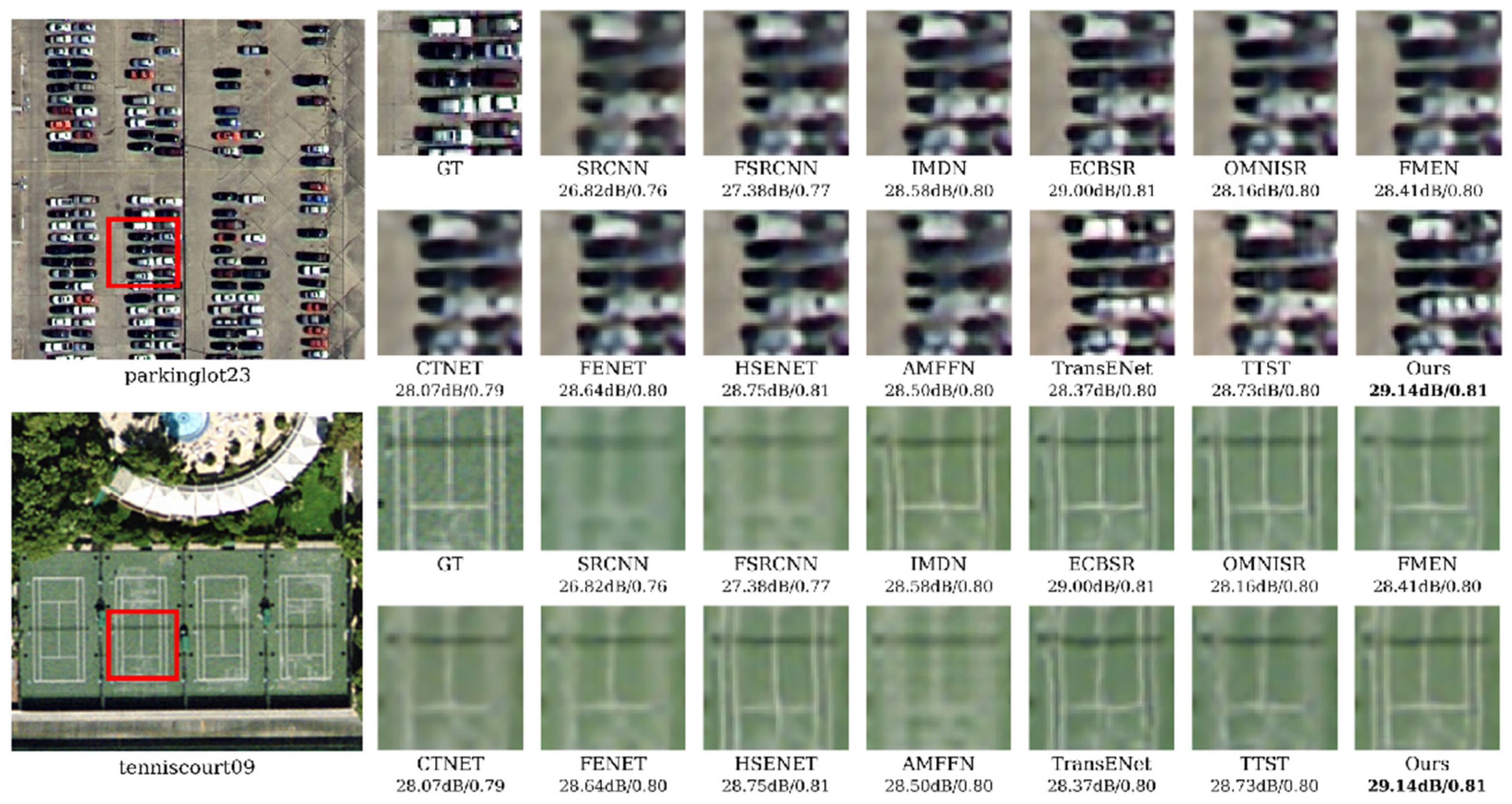
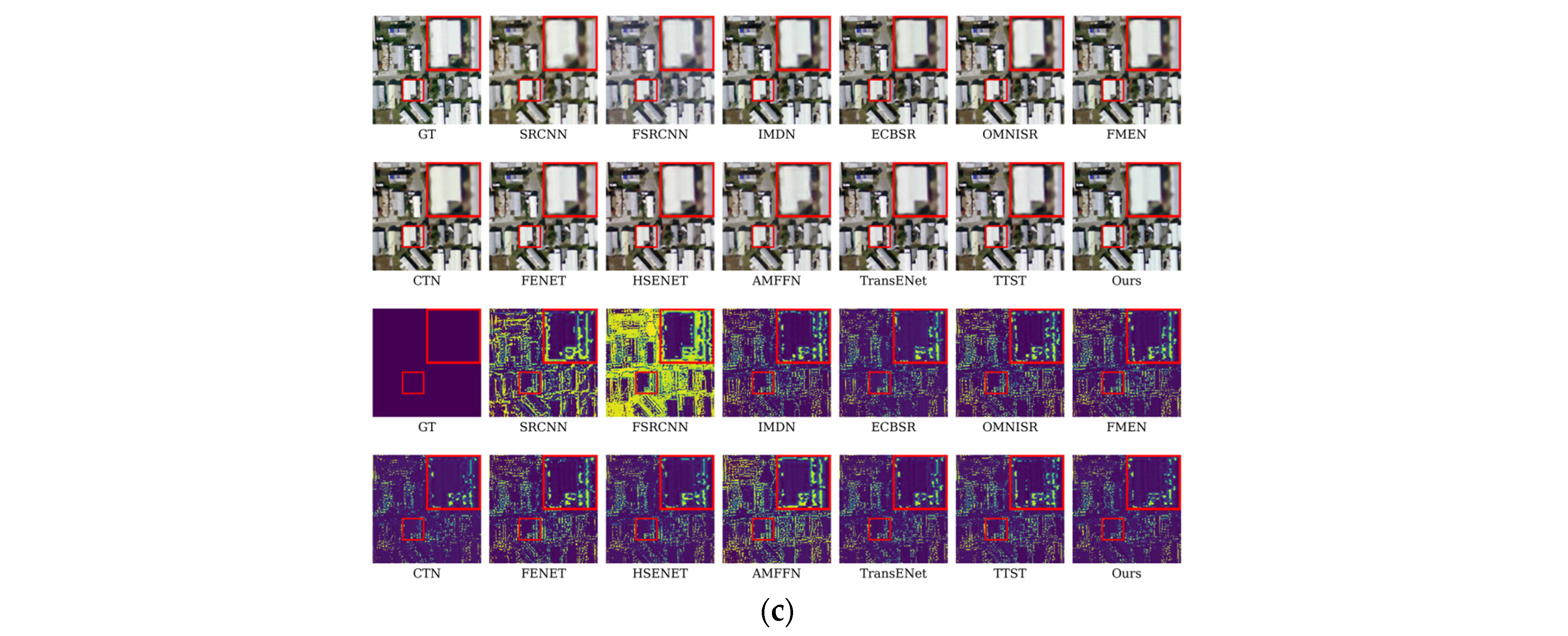
Figure 5 compares the reconstruction results of each model on the UCMerced dataset at scale ×4. The visual comparison clearly shows that DyLKANet excels at accurately capturing crucial high-frequency details in remote sensing images. Compared to other models, the image reconstructed by DyLKANet is closer to the real HR, with sharper edge contours and more detailed and accurate texture information. Notably, in the ×4 reconstruction of the parkinglot, only DyLKANet clearly reproduces the front and rear window details of the car.

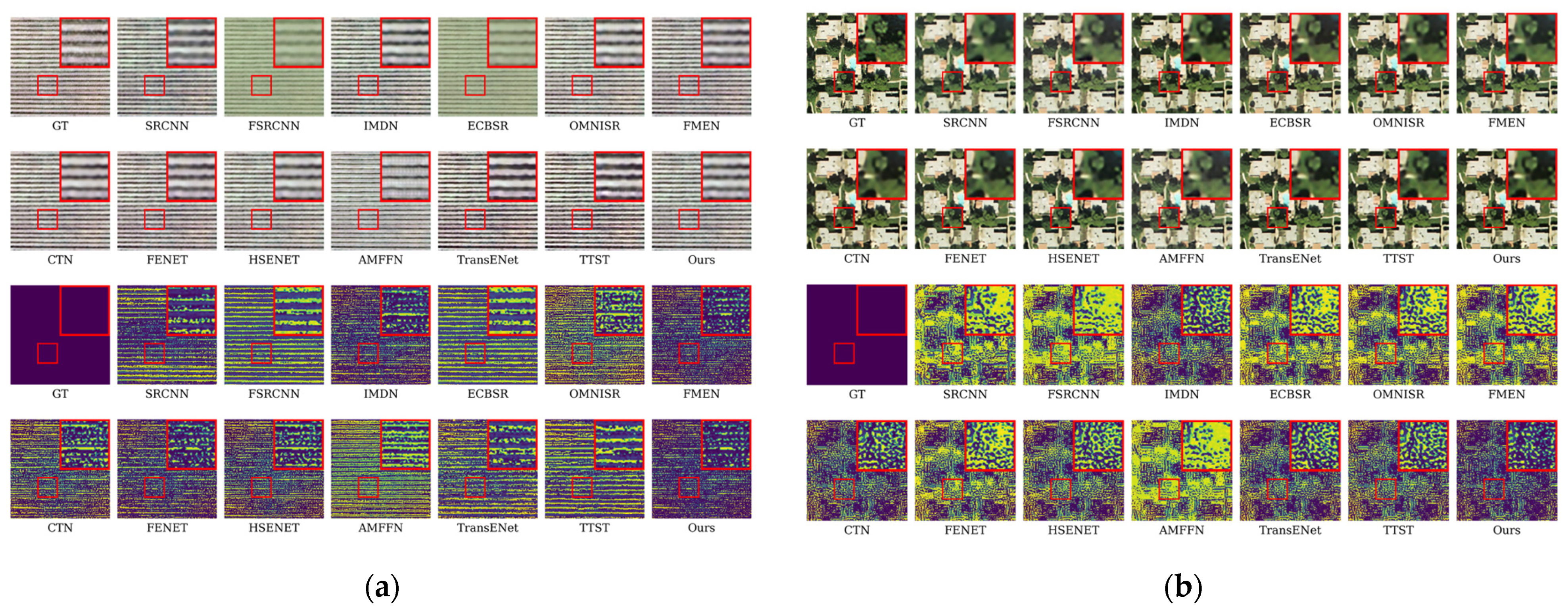
Figure 6 presents the residual visualization results of different models in the RSISR task. In the figure, yellow and blue regions, indicated by color bars, represent the mean square error (MSE) distribution between the super-resolution and ground truth images. Yellow indicates high MSE values (large error), while blue indicates low MSE values (small error). A comparison of the DyLKANet and AMFFN in Figure 6 reveals that DyLKANet has a larger blue area in the residual map, indicating superior performance in recovering details with lower MSE values. This comparison highlights the advantages of DyLKANet in the RSISR task, demonstrating that the proposed network structure more effectively captures and recovers high-frequency details.

3.5. Results of Experiments on AID Dataset

Table 3. PSNR and SSIM results of different methods on AID test dataset at scale ×2, ×3, and ×4.

Model	Year	Scale	Params [K]	FLops [G]	Memory [MB]	Time [ms]	AID
							PSNR	SSIM
SRCNN	2014	×2	69	7.1	22	0.187	32.326	0.906
FSRCNN	2016	×2	25	6.7	134	0.407	34.145	0.924
IMDN	2019	×2	694	70.7	70	5.536	34.921	0.928
ECBSR	2021	×2	1387	139.9	252	10.053	35.001	0.933
OMNISR	2023	×2	772	77.6	686	16.031	35.247	0.936
FMEN	2022	×2	325	33.2	32	2.413	34.912	0.914
CTNet	2021	×2	349	26.2	252	8.509	35.110	0.934
FENet	2022	×2	351	34.3	468	94.258	35.082	0.934
HSENET	2022	×2	5290	16.7	1816	7.352	35.050	0.934
AMFFN	2023	×2	298	26.8	362	12.938	35.214	0.935
TransENet	2022	×2	37,311	9.78	520	37.311	35.311	0.935
TTST	2024	×2	18,156	74.3	3480	113.442	35.282	0.936
Ours		×2	242	24.3	586	14.804	35.412	0.938
SRCNN	2014	×3	69	7.1	22	0.157	28.214	0.785
FSRCNN	2016	×3	25	13.7	136	0.391	30.183	0.832
IMDN	2019	×3	703	71.5	70	5.798	30.969	0.835
ECBSR	2021	×3	1571	159.6	252	10.975	30.726	0.843
OMNISR	2023	×3	780	78.5	686	15.240	31.190	0.855
FMEN	2022	×3	332	33.9	32	2.227	30.747	0.845
CTNet	2021	×3	349	36.6	252	9.818	30.885	0.849
FENet	2022	×3	357	35.0	468	94.269	29.857	0.834
HSENET	2022	×3	5470	17.4	1814	6.403	30.959	0.851
AMFFN	2023	×3	305	27.4	362	14.384	31.194	0.855
TransENet	2022	×3	37,495	14.3	432	37.495	30.700	0.844
TTST	2024	×3	18,341	75.1	3476	113.599	31.171	0.850
Ours		×3	248	25.0	588	15.052	31.362	0.859
SRCNN	2014	×4	69	7.1	22	0.149	26.302	0.697
FSRCNN	2016	×4	25	23.4	136	0.430	28.102	0.749
IMDN	2019	×4	715	72.8	70	5.773	28.730	0.762
ECBSR	2021	×4	1534	202.4	254	12.490	28.491	0.766
OMNISR	2023	×4	792	79.7	688	15.991	29.006	0.782
FMEN	2022	×4	341	34.8	34	2.642	28.515	0.765
CTNet	2021	×4	360	44.9	254	10.103	28.814	0.776
FENet	2022	×4	366	35.9	470	96.238	28.761	0.773
HSENET	2022	×4	5430	19.2	1816	6.276	28.743	0.773
AMFFN	2023	×4	314	28.4	364	26.455	29.034	0.783
TransENet	2022	×4	37,458	21.43	722	37.458	28.756	0.774
TTST	2024	×4	18,304	76.8	3480	112.150	28.476	0.778
Ours		×4	257	25.9	588	16.526	29.134	0.786

presents the PSNR and SSIM results for scales ×2, ×3, and ×4 on the AID dataset. DyLKANet demonstrates PSNR gains over suboptimal models across all scale combinations. Specifically, at the scale of ×2, compared to IMDN, ECBSR, OMNISR, and FMEN models, DyLKANet reduces parameters and computational complexity while improving PSNR by 0.16–0.50 dB and SSIM by 0.002–0.024. Compared to remote sensing super-resolution models, such as CTNet, FENet, HSENET, and AMFFN, DyLKANet improves PSNR by 0.19–0.36 dB and SSIM by 0.003–0.004. At the scale of ×3, DyLKANet increases PSNR by 0.168–0.662 dB and SSIM by 0.004–0.074. Compared to advanced remote sensing models like CTNet, it improves PSNR by 0.16–1.50 dB and SSIM by 0.004–0.025. At the scale of ×4 magnification, DyLKANet improves PSNR by 0.10–2.83 dB and SSIM by 0.003–0.089. Compared to CTNet and similar models, it achieves PSNR gains of 0.1–0.658 dB and SSIM gains of 0.003–0.013. While DyLKANet’s SSIM slightly decreases at the scale of ×4, its overall SSIM performance remains stable and comparable to or better than state-of-the-art models. These results indicate that DyLKANet performs well across various scale combinations, balancing parameter count and computational complexity while achieving comparable or superior performance to state-of-the-art models in PSNR and SSIM metrics.

Table 4. PSNR and SSIM results for 5 categories in the AID dataset using different methods, including ×2, ×3, and ×4.

Model	Scale	Image
		Bareland		Desert		Farmland		Playground		Bridge
		PSNR	SSIM	PSNR	SSIM	PSNR	SSIM	PSNR	SSIM	PSNR	SSIM
SRCNN	×2	38.851	0.894	43.347	0.967	35.824	0.911	30.496	0.880	32.831	0.910
FSRCNN	×2	39.421	0.899	44.032	0.971	37.167	0.926	32.310	0.900	36.417	0.945
IMDN	×2	40.645	0.902	44.901	0.976	38.121	0.939	33.765	0.923	37.559	0.954
ECBSR	×2	40.788	0.905	45.128	0.977	38.428	0.946	34.247	0.929	37.833	0.955
OMNISR	×2	40.698	0.903	44.895	0.976	38.115	0.939	33.797	0.923	37.567	0.954
FMEN	×2	40.696	0.903	44.866	0.975	38.081	0.937	33.843	0.923	37.588	0.954
CTNet	×2	40.782	0.905	45.153	0.977	38.270	0.941	33.922	0.925	37.674	0.955
FENet	×2	40.725	0.903	45.108	0.977	38.333	0.942	33.855	0.924	37.594	0.954
HSENET	×2	40.788	0.906	45.058	0.975	38.263	0.935	33.996	0.919	37.558	0.948
AMFFN	×2	40.789	0.909	45.147	0.975	38.392	0.939	34.012	0.926	37.559	0.949
TransENet	×2	39.426	0.905	39.801	0.974	38.104	0.936	33.733	0.916	37.341	0.947
TTST	×2	40.997	0.913	45.142	0.976	38.449	0.940	34.177	0.925	37.640	0.950
Ours	×2	40.947	0.912	45.382	0.978	38.482	0.944	34.352	0.923	37.943	0.951
SRCNN	×3	31.885	0.810	39.970	0.927	32.610	0.822	27.073	0.761	29.024	0.810
FSRCNN	×3	32.759	0.824	40.738	0.937	33.691	0.845	28.703	0.793	32.270	0.881
IMDN	×3	32.976	0.828	41.290	0.942	34.635	0.869	29.932	0.833	33.265	0.895
ECBSR	×3	33.045	0.830	41.547	0.945	34.104	0.881	30.520	0.847	33.488	0.899
OMNISR	×3	32.925	0.829	41.265	0.942	34.631	0.869	29.973	0.834	33.251	0.895
FMEN	×3	32.904	0.826	41.249	0.942	34.642	0.868	30.040	0.836	33.292	0.895
CTNet	×3	32.616	0.822	41.095	0.941	34.143	0.858	29.185	0.812	32.837	0.888
FENet	×3	33.011	0.830	41.524	0.945	34.771	0.873	29.975	0.835	33.297	0.895
HSENET	×3	38.474	0.931	41.539	0.943	34.903	0.867	30.377	0.830	33.421	0.885
AMFFN	×3	38.465	0.931	41.579	0.943	34.889	0.870	30.463	0.833	33.451	0.897
TransENet	×3	38.272	0.929	41.048	0.941	34.753	0.864	30.317	0.827	33.382	0.884
TTST	×3	38.334	0.932	41.446	0.939	34.852	0.871	30.418	0.841	33.441	0.896
Ours	×3	38.593	0.932	41.678	0.944	35.144	0.876	30.766	0.839	33.731	0.898
SRCNN	×4	32.038	0.833	38.415	0.896	31.321	0.764	25.499	0.675	27.198	0.734
FSRCNN	×4	34.723	0.874	39.157	0.908	32.152	0.786	26.900	0.708	29.916	0.815
IMDN	×4	35.390	0.882	39.588	0.913	33.028	0.814	27.879	0.753	30.846	0.835
ECBSR	×4	35.520	0.885	39.825	0.917	33.381	0.827	28.423	0.774	31.112	0.841
OMNISR	×4	35.360	0.882	39.081	0.911	32.874	0.808	27.739	0.746	30.614	0.827
FMEN	×4	35.381	0.882	39.550	0.912	32.963	0.810	27.911	0.755	30.827	0.835
CTNet	×4	35.156	0.879	38.917	0.909	32.352	0.792	27.193	0.723	30.182	0.817
FENet	×4	35.619	0.885	39.813	0.917	33.111	0.818	27.900	0.755	30.841	0.836
HSENET	×4	35.651	0.879	39.839	0.917	33.334	0.819	31.027	0.826	31.038	0.826
AMFFN	×4	35.639	0.885	39.907	0.918	33.383	0.821	28.530	0.764	31.054	0.844
TransENet	×4	35.591	0.879	39.363	0.916	33.354	0.822	28.613	0.766	31.274	0.831
TTST	×4	35.652	0.885	39.852	0.915	33.254	0.816	28.589	0.763	30.967	0.833
Ours	×4	35.724	0.888	39.988	0.922	33.497	0.824	28.621	0.767	31.383	0.847

presents five typical categories from the AID dataset—bareland, desert, farmland, playground, and bridge—to compare the performance of different SR models. As shown in Table 4, DyLKANet achieves the best average performance across all evaluation metrics, demonstrating its superior SR performance in remote sensing benchmarks for all categories. At scale ×2, DyLKANet achieves great PSNR values across most of the categories, with gains ranging from 0.033 dB to 0.23 dB. Similarly, the SSIM values range from an increase of 0.001 to 0.004. At scale ×3, DyLKANet achieves great average performance across all categories, with gains ranging from 0.099 dB to 0.243 dB. The SSIM values of DyLKANet range from an increase of 0.001 to 0.005. At scale ×4, DyLKANet achieves the highest PSNR values across all categories, highlighting its superior ability to recover image details. In the desert category, it achieves the highest increase in SSIM value of 0.004 compared to TTST.

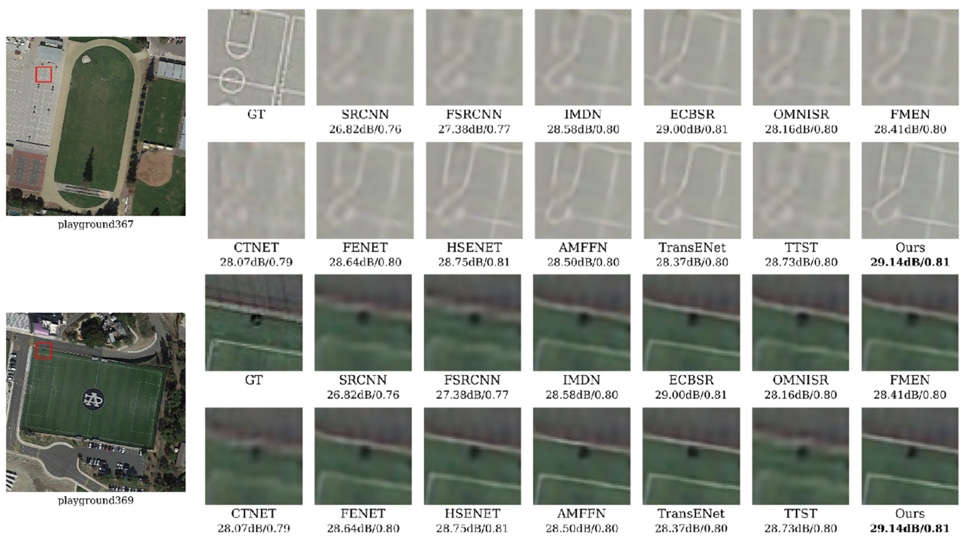
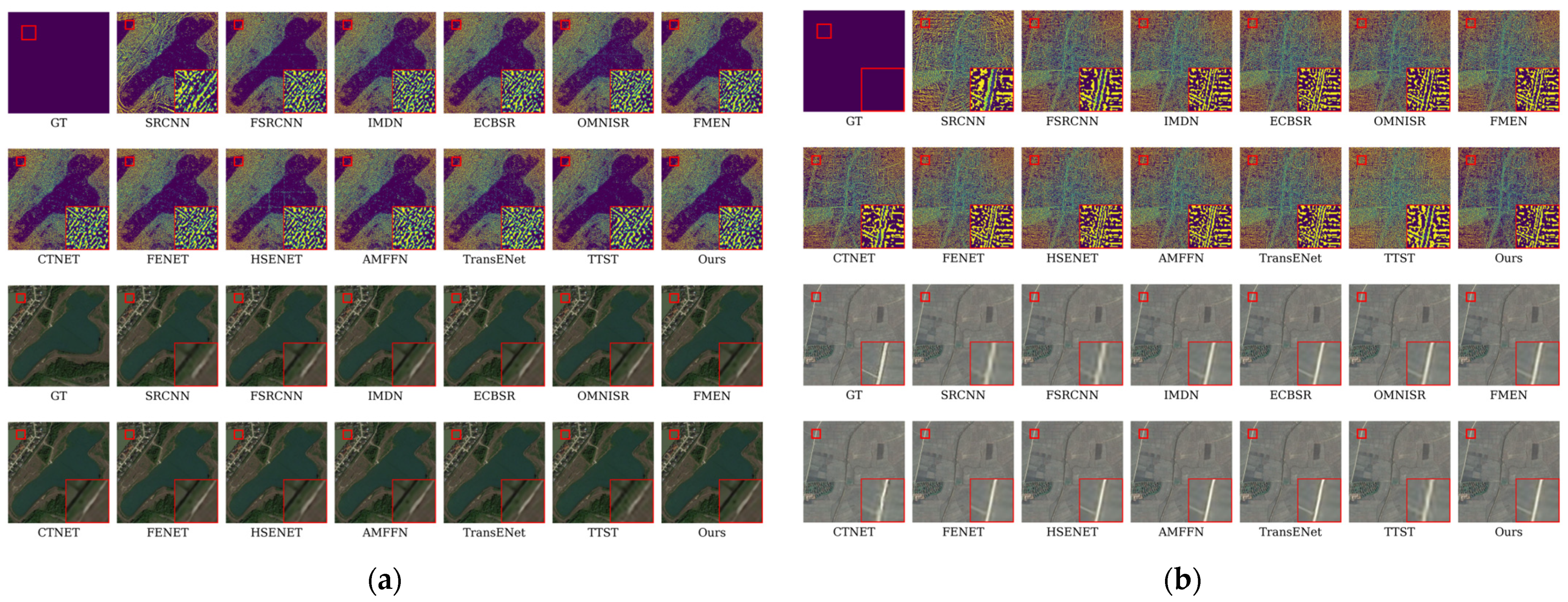
Figure 7 presents visual comparison results for a ×4 magnification factor. The figure illustrates qualitative results from test set samples of remote sensing images to compare different models in the SR task. The figure demonstrates that DyLKANet excels in recovering image edge textures. For instance, in the ×4 reconstruction of the playground, DyLKANet accurately recovers the regular lines, rendering them clear, coherent, and consistent with the real scene. In contrast, other SR models struggle with reconstruction, producing relatively blurred image details. This comparison highlights DyLKANet’s advantage in reconstructing fine details of remote sensing images. The comparison indicates that DyLKANet-reconstructed images exhibit rich edge textures and accurately capture key high-frequency details.

Figure 8 compares residual visualizations generated by various models for the remote sensing image super-resolution task on the AID dataset. The figure shows that compared to the AMFFN model, DyLKANet exhibits a larger blue area in the residual visualization, indicating superior detail reproduction in remote sensing images and a lower MSE value. In contrast, the residual visualization of AMFFN contains more yellow regions and higher MSE values. This suggests that DyLKANet more effectively captures high-frequency details in remote-sensing images.

3.6. Results of Experiments on DIV2K Dataset

To further validate the effectiveness and generalization ability of DyLKANet, experiments were conducted on the widely used DIV2K dataset at a scale of ×4. As illustrated in

Table 5. PSNR and SSIM results of different methods on DIV2K test dataset at scale ×4.

Model	Year	Scale	Params [K]	FLops [G]	Memory [MB]	Time [ms]	DIV2K
							PSNR	SSIM
SRCNN	2014	×4	69	7.1	22	0.149	26.829	0.762
FSRCNN	2016	×4	25	23.4	136	0.430	27.389	0.776
IMDN	2019	×4	715	72.8	70	5.773	28.580	0.808
ECBSR	2021	×4	1534	202.4	254	12.490	29.007	0.816
OMNISR	2023	×4	792	79.7	688	15.991	28.169	0.804
FMEN	2022	×4	341	34.8	34	2.642	28.410	0.804
CTNet	2021	×4	360	44.9	254	10.103	28.078	0.792
FENet	2022	×4	366	35.9	470	96.238	28.646	0.809
HSENET	2022	×4	5430	19.2	1816	6.276	28.754	0.815
AMFFN	2023	×4	314	28.4	364	26.455	28.504	0.806
TransENet	2022	×4	37,458	21.43	722	37.458	28.379	0.804
TTST	2024	×4	18,304	76.8	3480	112.150	28.732	0.808
Ours		×4	257	25.9	588	16.526	29.148	0.819

, Compared to HSENET, DyLKANet achieves a 95.26% reduction in parameter count. It also reduces the computational complexity by 66.27% compared to TTST. Although the inference time of DyLKANet has increased slightly compared to the RSISR model HSENET, it remains lower than that of the other five RSISR models. Specifically, DyLKANet achieves a higher PSNR (29.148 dB) and SSIM (0.819). This demonstrates the efficiency and effectiveness of DyLKANet in achieving high-quality super-resolution with a much lighter model architecture.

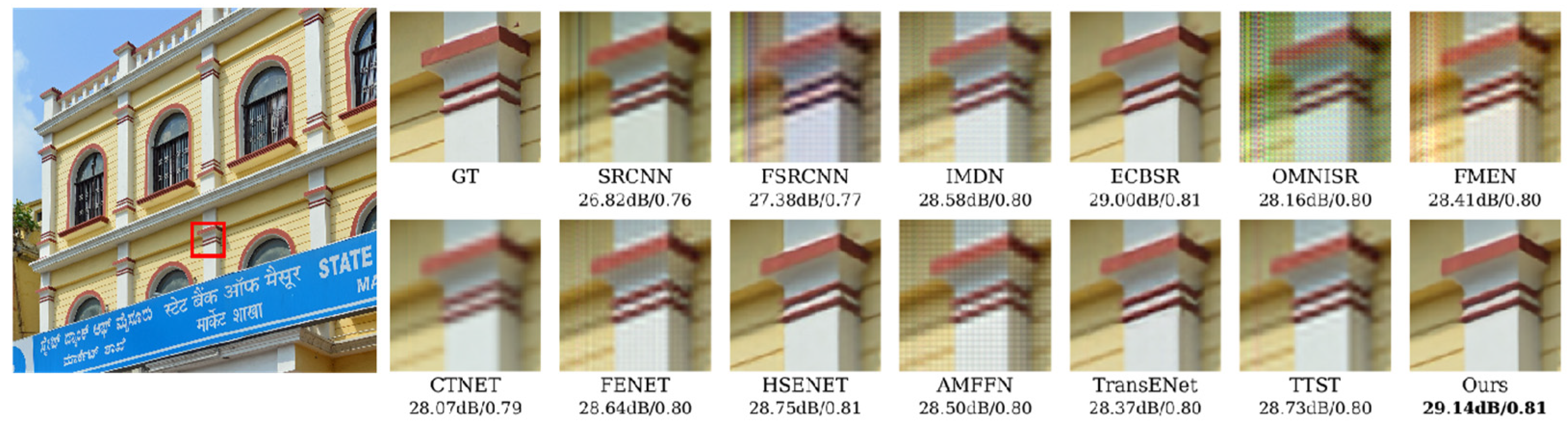
Figure 9 presents a visual comparison of ×4 super-resolution results on the DIV2K. The image shows a comparison of various image restoration models, highlighting the performance of the proposed model in restoring image details and clarity. Subjectively, the proposed model recovers more precise details of the columns and walls compared to other models, and objectively, it outperforms in metrics such as dB and SSIM values. This indicates the superior performance of the proposed model in image restoration tasks.

4. Ablation Experiments and Discussions

This section analyzes the impact of the key modules of DyLKANet and its variants. For this purpose, we selected the UCMerced dataset and trained all models with a ×4 scale factor to ensure the reliability of the analysis and conclusions.

4.1. Effectiveness of the Feature Distillation and Enhancement Blocks

To evaluate the effectiveness of the FDEB, a comparison experiment was conducted. In the experiment, the feature distillation stage of FDEB was replaced with three standard convolutional layers, and this modified block was used as the core component of the network. The experimental results are presented in

Table 6. Effectiveness of FDEB on the UC Merced test dataset for ×4.

Settings	FDEB	CFFM	Params [K]	FLops [G]	PSNR	SSIM
1	×	×	412	42.3	27.04	0.733
2	√	×	317	28.5	28.05	0.748
3	×	√	431	41.4	28.08	0.751
4	√	√	257	25.9	28.16	0.774

. Analysis of the first two rows in Table 6 indicates that integrating FDEB not only enables a lighter network architecture but also significantly enhances reconstruction accuracy. Specifically, the network parameters are reduced to 257 K, while the PSNR increases by 0.08 dB and the SSIM improves by 0.023. These metric improvements demonstrate the effectiveness of FDEB in preserving image details and enhancing image quality.

To comprehensively demonstrate the impact of FDEB, a visual analysis was conducted using the Local Attribute Map (LAM) [49]. Figure 10 illustrates that integrating FDEB increases the diffusion index (DI) value from 1.73 to 3.07. The DI metric quantifies pixel engagement, where a higher DI indicates a broader scope of attention. Furthermore, the improved SR results reinforce the effectiveness of FDEB. Collectively, these advancements underscore the superiority of FDEB.

4.2. Analysis of the Number of FDEB Modules

To fine-tune network parameters and performance, we investigate how the number of FDEBs affects overall network performance, as these blocks are critical to the architecture and directly influence the final outcome. During the evaluation, we consider both performance improvement and the constraints of parameter size (Params) and computational complexity (measured by FLops). As shown in

Table 7. Performance results with different settings of n on the UCMerced dataset at scale ×4.

Settings	Params [K]	FLops [G]	PSNR	SSIM
2	153	11.6	27.96	0.770
4	187	19.7	28.01	0.771
6	257	25.9	28.16	0.774
8	289	27.1	28.14	0.772
10	392	27.7	28.10	0.771

, we tested varying numbers of FDEBs (from 2 to 10) and recorded the corresponding performance metrics. The results indicate that at lower values of n, the network’s performance (measured by PSNR and SSIM) improves significantly, demonstrating a clear positive correlation. Performance peaks at n = 6, with the PSNR reaching its maximum value of 28.16 and SSIM stabilizing at a high level. Beyond n = 6, performance indicators stabilize with no significant improvement, suggesting saturation in network performance. Additionally, as the number of FDEBs increases, both parameter size and computational complexity increase proportionally. Specifically, as n increases from 2 to 10, network parameters rise from 153 K to 392 K, while computational complexity grows from 11.6 G to 27.7 G. Given the goal of developing a lightweight RSISR technique, we prioritize configurations with fewer parameters and reduced computation when performance is comparable. After balancing performance and lightweight design, we determine n = 6 as the optimal network configuration. At n = 6, the network achieves high performance while effectively controlling parameter size and computational complexity.

4.3. Effectiveness of CFFM

To quantitatively assess the effectiveness of the CFFM, we performed a comprehensive comparative analysis with several other feature fusion structures (as shown in Figure 11), each regarded as a core network component.

Table 8. Performance results with different fusion structures on the UC Merced test dataset for ×4 SR.

Variant	Params [K]	FLops [G]	PSNR	SSIM
a	607	26.8	27.44	0.7645
b	314	28.4	28.03	0.7701
c	366	35.9	27.56	0.7526
d	257	25.9	28.16	0.7743

presents the performance metrics of various structures, including parameters (Params), computational complexity (FLops), PSNR, and SSIM.

The multi-level feature fusion strategy in DyLKANet, as illustrated in Figure 11d, integrates features from different levels to enhance the quality of the reconstructed image. Compared to MSRN (Figure 11a), which employs a standard feature fusion structure, DyLKANet reduces the number of parameters by 57.67%. When compared to AMFFN (Figure 11b), which uses a multi-level feature fusion module, DyLKANet’s CFFM demonstrates superior performance in terms of parameter efficiency and computational complexity, achieving a Peak Signal-to-Noise Ratio (PSNR) of 28.16 dB and a Structural Similarity Index (SSIM) of 0.7743 with only 257 K parameters and 25.9 G FLOPs. Compared to FENET (Figure 11c), which utilizes a reverse fusion module, DyLKANet reduces the number of parameters by 21%.

4.4. Effectiveness of LK-CSA

To evaluate the LK-CSA module’s contribution to model performance, we constructed two model sets: one including the LK or CSA module (“w”) and one without it (“w/o”), keeping all other components and configurations identical.

Table 9. Performance results with different settings on the ucmerced test dataset for ×4 SR.

Settings	Params [K]	FLops [G]	PSNR	SSIM
w LKA + CSA	257	25.9	28.16	0.774
w LKA	239	26.1	27.57	0.770
w CSA	232	26.7	27.84	0.770
w/o LKA + CSA	230	24.6	26.62	0.713

indicates that incorporating the LK-CSA module reduces model parameters by approximately 21% (from 312 K to 257 K) while significantly improving performance. Specifically, the LK-CSA-equipped model improved PSNR by 1.54dB (from 26.62 to 28.16) and SSIM by 0.061 (from 0.713 to 0.774). These results demonstrate the LK-CSA module’s effectiveness in enhancing performance and its importance in resource-constrained environments. Specifically, combining LKA and CSA may improve efficiency in feature extraction and information fusion compared to using either module alone, enhancing the model’s capacity to process complex data structures.

To evaluate the effectiveness of different attention mechanisms, we conducted experiments with various combinations of attention modules. The results are presented in

Table 10. Performance results with different attentions on the ucmerced test dataset for ×4 SR.

Attentions	Params [K]	FLops [G]	PSNR	SSIM
w ESA + CA	265	27.5	27.89	0.770
w ESA + LKA	255	26.5	28.02	0.770
w ESA + CSA	257	25.9	28.14	0.774
w CA + LKA	253	26.0	28.05	0.771
w LKA + CSA	257	25.9	28.16	0.774

, which includes the number of parameters, computational complexity (FLops), PSNR, and SSIM for each configuration. Compared to the baseline model, the combination of ESA and CA results in a moderate reduction in parameters and computational complexity. However, the PSNR and SSIM values are slightly lower than those achieved with LKA and CSA, indicating that this combination is less effective in capturing long-range dependencies and refining feature representations. The LKA + CSA combination achieves the highest PSNR and SSIM values in the test configuration. The LKA module effectively captures long-term dependencies, while the CSA module further refines feature representations to achieve optimal overall performance.

4.5. Effectiveness of DyConv

In this section, we further analyze the advantages of the dynamic convolutional residual block (DCRB) with dynamic convolution (DyConv) compared to static convolution. The experimental results in

Table 11. Quantitative comparison of different convolution decomposition approaches.

Settings	Params [K]	FLops [G]	PSNR	SSIM
w DyConv	257	25.9	28.16	0.774
w Conv	276	28.1	28.02	0.772

provide a clear comparison between models with DyConv and with static convolution.

As shown in Table 11, the model with DyConv (“w DyConv”) has 257 K parameters and 25.9 G FLOPs, while the model with static convolution (“w Conv”) has 276 K parameters and 28.1 G FLOPs. This indicates that the use of DyConv reduces the number of parameters by approximately 7.6% (from 276 K to 257 K) and the computational complexity by approximately 7.8% (from 28.1 G to 25.9 G). Despite the reduction in parameters and computational complexity, the model with DyConv demonstrates improved performance in terms of PSNR and SSIM. Specifically, the model with DyConv achieves a PSNR of 28.16 dB and an SSIM of 0.774, while the model with static convolution achieves a PSNR of 28.02 dB and an SSIM of 0.772. This indicates that DyConv not only reduces the computational overhead but also enhances the model’s ability to reconstruct high-quality images.

The advantages of DyConv can be attributed to its ability to dynamically generate convolution kernels based on the input features. This dynamic adjustment allows the model to adaptively capture the most relevant features for each input sample, leading to more efficient and effective feature extraction. In contrast, static convolution uses fixed convolution kernels that may not be optimal for all input samples, leading to redundant computations and less effective feature extraction.

4.6. Analysis of the Number of Layers of DyConv

To further analyze the impact of the number of layers in the dynamic convolutional residual block (DCRB) on the performance of DyLKANet, we conducted an ablation study with different numbers of layers (1, 5, 7, 13, 15). The results are presented in

Table 12. Performance results with different numbers of layers in DyConv on the UCMerced test dataset for ×4 SR.

Number of Layers	Params [K]	FLops [G]	PSNR	SSIM
1	230	23.8	27.66	0.763
5	276	24.6	27.97	0.769
7	257	25.9	28.16	0.774
13	320	28.1	28.12	0.772
15	345	32.5	28.07	0.770

. The results indicate that the number of layers in the DyConv has a significant impact on the performance of DyLKANet. While increasing the number of layers generally improves the model’s ability to capture complex features, there is an optimal point beyond which adding more layers leads to diminishing returns or even performance degradation. The optimal number of layers appears to be around 7, where the model achieves the highest PSNR and SSIM values while maintaining a reasonable computational complexity. Further increasing the number of layers beyond this point results in decreased performance, likely due to overfitting or the increased computational burden.

4.7. Models Efficiency

To comprehensively evaluate model efficiency, we introduce inference time, memory consumption, parameters, and FLops as intuitive metrics and present a comparative analysis in Figure 12a–d. Figure 12a illustrates the inference times of different models, showing that DyLKANet achieves a relatively low inference time compared to other state-of-the-art models. Specifically, DyLKANet outperforms the heavily parameterized HSENET, achieving a 0.557 dB improvement in PSNR while maintaining similar model complexity. This performance enhancement is accompanied by a slight increase in inference time (approximately 21.2 ms for 100 images), which remains within an acceptable range, demonstrating DyLKANet’s efficiency. Figure 12b visualizes the memory consumption of different models, indicating that DyLKANet has a moderate memory footprint, making it suitable for deployment on devices with limited memory resources. Figure 12c shows the trade-off between PSNR and the number of parameters. DyLKANet achieves a high PSNR with a relatively low number of parameters, indicating its effectiveness in balancing performance and model size. This balance is crucial for practical deployment, as it allows for high-quality super-resolution without the need for excessive computational resources. Figure 12d presents the FLops of different models, highlighting DyLKANet’s low computational complexity. DyLKANet has a significantly lower GFLOP count compared to models like HSENET, making it more efficient in terms of computational requirements. This is particularly important for real-world applications where computational resources are limited, such as edge devices.

5. Limitations and Future Work

DyLKANet, while reducing parameters to meet the demands of lightweight applications, is able to achieve super-resolution results comparable to state-of-the-art models. Although DyLKANet has significantly reduced the number of parameters and computational complexity, there is still room for further optimization. In the future, we will leverage techniques such as pre-training and LoRA to reduce model size, while also decreasing GPU memory usage and maintaining inference efficiency during deployment. Currently, DyLKANet has been tested on visible light remote sensing images, but further optimization and improvements are needed to enhance the network’s ability to handle extremely low-resolution images and remote sensing images of other modalities. Additionally, the degradation model is one of the key issues that need to be addressed in remote sensing super-resolution. In this paper, a fixed degradation model similar to those used in most studies is still adopted, which may not fully capture the diverse degradation patterns encountered in real-world remote sensing images. Future research needs to explore more sophisticated training methods, such as self-supervised or unsupervised learning, to improve the model’s robustness and generalization ability across different degradation scenarios. Lastly, the evaluation of DyLKANet has primarily been conducted on publicly available datasets, which may not fully represent the complexity and diversity of real-world remote sensing data. Future work should include more comprehensive testing on a wider range of datasets, including those with varying levels of noise, blur, and other degradation factors, to better assess the model’s performance in practical applications.

6. Conclusions

This paper proposes a dynamic distillation network, DyLKANet, to address the challenge of remote sensing image super-resolution. The network leverages a large-kernel attention mechanism to achieve efficient feature extraction and capture global dependencies through a multi-level feature fusion strategy. Experimental results show that DyLKANet performs comparably to state-of-the-art methods on the publicly available UCMerced, AID, and DIV2K datasets, while maintaining low parameter count and computational complexity. Specifically, on the UCMerced dataset, DyLKANet improves the PSNR by 0.212 dB and 0.151 dB over the suboptimal TTST at the scale of ×2 and ×4 scaling factors, respectively. At the scale of ×2, DyLKANet improves PSNR by 0.439–0.589 dB, SSIM by 0.006–0.010, and reduces parameters by 25.54–82.57% compared to natural image super-resolution models. Compared to remote sensing super-resolution models, DyLKANet improves PSNR by 0.212–0.576 dB, SSIM by 0.005–0.009, and reduces parameters by 18.79–95.46%. DyLKANet reduces FLops operations by 7.25–67.30%. Furthermore, ablation experiments validate the effectiveness of key modules, including FDEB, CFFM, and dynamic convolution. Results show that these modules significantly enhance model performance while reducing parameter count and computational complexity. In conclusion, DyLKANet, a lightweight super-resolution network for remote sensing images, demonstrates significant potential in resource-constrained environments.

References

1. Liu, H.; Qian, Y.; Zhong, X.; Chen, L.; Yang, G. Research on super-resolution reconstruction of remote sensing images: A comprehensive review. Opt. Eng. 2021, 60, 100901. [Google Scholar] [CrossRef]
2. Wang, Z.; Chen, J.; Hoi, S.C. Deep learning for image super-resolution: A survey. IEEE Trans. Pattern Anal. Mach. Intell. 2020, 43, 3365–3387. [Google Scholar] [CrossRef] [PubMed]
3. Zhu, F. A review of deep learning based image super-resolution techniques. arXiv 2022, arXiv:2201.10521. [Google Scholar] [CrossRef]
4. Hayat, M.; Aramvith, S.; Achakulvisut, T. SEGSRNet for Stereo-Endoscopic Image Super-Resolution and Surgical Instrument Segmentation. arXiv 2024, arXiv:2404.13330v2. [Google Scholar]
5. Ahmad, N.; Strand, R.; Sparresäter, B.; Tarai, S.; Lundström, E.; Bergström, G.; Ahlström, H.; Kullberg, J. Automatic segmentation of large-scale CT image datasets for detailed body composition analysis. BMC Bioinform. 2023, 24, 346. [Google Scholar] [CrossRef] [PubMed]
6. Dong, C.; Loy, C.C.; He, K.; Tang, X. Learning a deep convolutional network for image super-resolution. In Proceedings of the Computer Vision—ECCV 2014: 13th European Conference, Zurich, Switzerland, 6–12 September 2014; pp. 184–199. [Google Scholar] [CrossRef]
7. Yang, H.; Yang, X.; Liu, K.; Jeon, G.; Zhu, C. SCN: Self-Calibration Network for fast and accurate image super-resolution. Expert Syst. Appl. 2023, 226, 120159. [Google Scholar] [CrossRef]
8. Dong, C.; Loy, C.C.; Tang, X. Accelerating the super-resolution convolutional neural network. In Proceedings of the Computer Vision–ECCV 2016: 14th European Conference, Amsterdam, The Netherlands, 11–14 October 2016; Proceedings, Part II 14. pp. 391–407. [Google Scholar] [CrossRef]
9. Kim, J.; Lee, J.K.; Lee, K.M. Accurate image super-resolution using very deep convolutional networks. In Proceedings of the IEEE Conference on Computer Vision and Pattern Recognition, Las Vegas, NV, USA, 27–30 June 2016; pp. 1646–1654. [Google Scholar] [CrossRef]
10. Lai, W.S.; Huang, J.B.; Ahuja, N.; Yang, M.H. Deep laplacian pyramid networks for fast and accurate super-resolution. In Proceedings of the IEEE Conference on Computer Vision and Pattern Recognition, Honolulu, HI, USA, 21–26 July 2017; pp. 624–632. [Google Scholar] [CrossRef]
11. Lim, B.; Son, S.; Kim, H.; Nah, S.; Mu Lee, K. Enhanced deep residual networks for single image super-resolution. In Proceedings of the IEEE Conference on Computer Vision and Pattern Recognition Workshops, Honolulu, HI, USA, 21–26 July 2017; pp. 136–144. [Google Scholar] [CrossRef]
12. Kim, J.; Lee, J.K.; Lee, K.M. Deeply-recursive convolutional network for image super-resolution. In Proceedings of the IEEE Conference on Computer Vision and Pattern Recognition (CVPR), Las Vegas, NV, USA, 27–30 June 2016; pp. 1637–1645. [Google Scholar] [CrossRef]
13. Tai, Y.; Yang, J.; Liu, X. Image super-resolution via deep recursive residual network. In Proceedings of the IEEE Conference on Computer Vision and Pattern Recognition (CVPR), Honolulu, HI, USA, 21–26 July 2017; pp. 2790–2798. [Google Scholar] [CrossRef]
14. Tong, T.; Li, G.; Liu, X.; Gao, Q. Image super-resolution using dense skip connections. In Proceedings of the IEEE International Conference on Computer Vision (ICCV), Venice, Italy, 22–29 October 2017; pp. 4809–4817. [Google Scholar] [CrossRef]
15. Zhang, Y.; Tian, Y.; Kong, Y.; Zhong, B.; Fu, Y. Residual dense network for image super-resolution. In Proceedings of the IEEE/CVF Conference on Computer Vision and Pattern Recognition, Salt Lake City, UT, USA, 18–23 June 2018; pp. 2472–2481. [Google Scholar] [CrossRef]
16. Ledig, C.; Theis, L.; Huszár, F.; Caballero, J.; Cunningham, A.; Acosta, A.; Aitken, A.; Tejani, A.; Totz, J.; Wang, Z.; et al. Photo-realistic single image super-resolution using a generative adversarial network. In Proceedings of the IEEE Conference on Computer Vision and Pattern Recognition, Honolulu, HI, USA, 21–26 July 2017; pp. 4681–4690. [Google Scholar] [CrossRef]
17. Shang, T.; Dai, Q.; Zhu, S.; Yang, T.; Guo, Y. Perceptual extreme super-resolution network with receptive field block. In Proceedings of the IEEE/CVF Conference on Computer Vision and Pattern Recognition Workshops, Seattle, WA, USA, 14–19 June 2020; pp. 440–441. [Google Scholar] [CrossRef]
18. Dai, T.; Cai, J.; Zhang, Y.; Xia, S.T.; Zhang, L. Second-order attention network for single image super-resolution. In Proceedings of the IEEE/CVF Conference on Computer Vision and Pattern Recognition, Long Beach, CA, USA, 15–20 June 2019; pp. 11065–11074. [Google Scholar] [CrossRef]
19. Zhou, Y.; Li, Z.; Guo, C.L.; Bai, S.; Cheng, M.M.; Hou, Q. SRformer: Permuted self-attention for single image super-resolution. In Proceedings of the IEEE/CVF International Conference on Computer Vision, Paris, France, 1–16 October 2023; pp. 12780–12791. [Google Scholar] [CrossRef]
20. Zhou, Y.; Wu, G.; Fu, Y.; Li, K.; Liu, Y. Cross-MPI: Cross-scale stereo for image super-resolution using multiplane images. In Proceedings of the IEEE/CVF Conference on Computer Vision and Pattern Recognition, Nashville, TN, USA, 20–25 June 2021; pp. 14842–14851. [Google Scholar] [CrossRef]
21. Son, S.; Lee, K.M. SRWARP: Generalized image super-resolution under arbitrary transformation. In Proceedings of the IEEE/CVF Conference on Computer Vision and Pattern Recognition, Nashville, TN, USA, 20–25 June 2021; pp. 7782–7791. [Google Scholar] [CrossRef]
22. Hui, Z.; Gao, X.; Yang, Y.; Wang, X. Lightweight image super-resolution with information multi-distillation network. In Proceedings of the 27th Acm International Conference on Multimedia, New York, NY, USA, 21–25 October 2019; pp. 2024–2032. [Google Scholar] [CrossRef]
23. Zhang, X.; Zeng, H.; Zhang, L. Edge-oriented convolution block for real-time super resolution on mobile devices. In Proceedings of the 29th ACM International Conference on Multimedia, Chengdu, China, 20–24 October 2021; pp. 4034–4043. [Google Scholar] [CrossRef]
24. Du, Z.; Liu, D.; Liu, J.; Tang, J.; Wu, G.; Fu, L. Fast and memory-efficient network towards efficient image super-resolution. In Proceedings of the IEEE/CVF Conference on Computer Vision and Pattern Recognition, New Orleans, LA, USA, 18–24 June 2022; pp. 853–862. [Google Scholar] [CrossRef]
25. Wang, Y.; Jin, S.; Yang, Z.; Guan, H.; Ren, Y.; Cheng, K.; Zhao, X.; Liu, X.; Chen, M.; Liu, Y.; et al. TTSR: A transformer-based topography neural network for digital elevation model super-resolution. IEEE Trans. Geosci. Remote Sens. 2024, 62, 4403719. [Google Scholar] [CrossRef]
26. Lu, Z.; Li, J.; Liu, H.; Huang, C.; Zhang, L.; Zeng, T. Transformer for single image super-resolution. In Proceedings of the IEEE/CVF Conference on Computer Vision and Pattern Recognition Workshops (CVPRW), New Orleans, LA, USA, 19–20 June 2022; pp. 456–465. [Google Scholar] [CrossRef]
27. Liang, J.; Cao, J.; Sun, G.; Zhang, K.; Van Gool, L.; Timofte, R. SwinIR: Image restoration using swin transformer. In Proceedings of the IEEE/CVF International Conference on Computer Vision, Montreal, BC, Canada, 11–17 October 2021; pp. 1833–1844. [Google Scholar] [CrossRef]
28. Xiao, Y.; Yuan, Q.; Jiang, K.; He, J.; Wang, Y.; Zhang, L. From degrade to upgrade: Learning a self-supervised degradation guided adaptive network for blind remote sensing image super-resolution. Inf. Fusion 2023, 96, 297–311. [Google Scholar] [CrossRef]
29. Qin, M.; Mavromatis, S.; Hu, L.; Zhang, F.; Liu, R.; Sequeira, J.; Du, Z. Remote sensing single-image resolution improvement using a deep gradient-aware network with image-specific enhancement. Remote Sens. 2020, 12, 758. [Google Scholar] [CrossRef]
30. Li, Q.; Yuan, Y.; Jia, X.; Wang, Q. Dual-stage approach toward hyperspectral image super-resolution. IEEE Trans. Image Process. 2022, 31, 7252–7263. [Google Scholar] [CrossRef]
31. Dong, R.; Mou, L.; Zhang, L.; Fu, H.; Zhu, X.X. Real-world remote sensing image super-resolution via a practical degradation model and a kernel-aware network. ISPRS J. Photogramm. Remote Sens. 2022, 191, 155–170. [Google Scholar] [CrossRef]
32. Ahn, N.; Kang, B.; Sohn, K.A. Fast, accurate, and lightweight super-resolution with cascading residual network. In Proceedings of the European Conference on Computer Vision (ECCV), Munich, Germany, 8–14 September 2018; pp. 252–268. [Google Scholar] [CrossRef]
33. Yang, B.; Bender, G.; Le, Q.V.; Ngiam, J. Condconv: Conditionally parameterized convolutions for efficient inference. In Advances in Neural Information Processing Systems; The MIT Press: Cambridge, MA, USA, 2019; p. 32. [Google Scholar] [CrossRef]
34. Wang, S.; Zhou, T.; Lu, Y.; Di, H. Contextual transformation network for lightweight remote-sensing image super-resolution. IEEE Trans. Geosci. Remote Sens. 2021, 60, 5615313. [Google Scholar] [CrossRef]
35. Wang, Z.; Li, L.; Xue, Y.; Jiang, C.; Wang, J.; Sun, K.; Ma, H. FeNet: Feature enhancement network for lightweight remote-sensing image super-resolution. IEEE Trans. Geosci. Remote Sens. 2022, 60, 5615313. [Google Scholar] [CrossRef]
36. Li, W.; Zhou, K.; Qi, L.; Jiang, N.; Lu, J.; Jia, J. LAPAR: Linearly-assembled pixel-adaptive regression network for single image super-resolution and beyond. Adv. Neural Inf. Process. Syst. 2020, 33, 20343–20355. [Google Scholar] [CrossRef]
37. Qin, J.; Liu, F.; Liu, K.; Jeon, G.; Yang, X. Lightweight hierarchical residual feature fusion network for single-image super-resolution. Neurocomputing 2022, 478, 104–123. [Google Scholar] [CrossRef]
38. Liu, F.; Yang, X.; De Baets, B. A deep recursive multi-scale feature fusion network for image super-resolution. J. Vis. Commun. Image Represent. 2023, 90, 103730. [Google Scholar] [CrossRef]
39. Wang, H.; Cheng, S.; Li, Y.; Du, A. Lightweight Remote-Sensing Image Super-Resolution via Attention-Based Multilevel Feature Fusion Network. IEEE Trans. Geosci. Remote Sens. 2023, 61, 2005715. [Google Scholar] [CrossRef]
40. Park, K.; Soh, J.W.; Cho, N.I. A dynamic residual self-attention network for lightweight single image super-resolution. IEEE Trans. Multimed. 2023, 25, 907–918. [Google Scholar] [CrossRef]
41. Wang, H.; Chen, X.; Ni, B.; Liu, Y.; Liu, J. Omni aggregation networks for lightweight image super-resolution. In Proceedings of the IEEE/CVF Conference on Computer Vision and Pattern Recognition, Vancouver, BC, Canada, 17–24 June 2023; pp. 22378–22387. [Google Scholar] [CrossRef]
42. Zhang, X.; Zeng, H.; Guo, S.; Zhang, L. Efficient long-range attention network for image super-resolution. In Proceedings of the European Conference on Computer Vision; Springer Nature: Cham, Switzerland, 2022; pp. 649–667. [Google Scholar] [CrossRef]
43. Xie, C.; Zhang, X.; Li, L.; Meng, H.; Zhang, T.; Li, T.; Zhao, X. Large kernel distillation network for efficient single image super-resolution. In Proceedings of the IEEE/CVF Conference on Computer Vision and Pattern Recognition, Vancouver, BC, Canada, 17–24 June 2023; pp. 1283–1292. [Google Scholar] [CrossRef]
44. Luo, P.; Xiao, G.; Gao, X.; Wu, S. LKD-Net: Large kernel convolution network for single image dehazing. In Proceedings of the 2023 IEEE International Conference on Multimedia and Expo (ICME), Brisbane, Australia, 10–14 July 2023; pp. 1601–1606. [Google Scholar] [CrossRef]
45. Choi, H.; Lee, J.; Yang, J. N-gram in swin transformers for efficient lightweight image super-resolution. In Proceedings of the IEEE/CVF Conference on Computer Vision and Pattern Recognition, Vancouver, BC, Canada, 17–24 June 2023; pp. 2071–2081. [Google Scholar] [CrossRef]
46. Li, J.; Fang, F.; Mei, K.; Zhang, G. Multi-scale residual network for image super-resolution. In Proceedings of the European Conference on Computer Vision (ECCV), Munich, Germany, 8–14 September 2018. [Google Scholar] [CrossRef]
47. Yang, Y.; Newsam, S. Bag-of-visual-words and spatial extensions for land-use classification. In Proceedings of the 18th SIGSPATIAL International Conference on Advances in Geographic Information Systems, San Jose, CA, USA, 3–5 November 2010; pp. 270–279. [Google Scholar] [CrossRef]
48. Xia, G.S.; Hu, J.; Hu, F.; Shi, B.; Bai, X.; Zhong, Y.; Zhang, L.; Lu, X. AID: A Benchmark Data Set for Performance Evaluation of Aerial Scene Classification. IEEE Trans. Geosci. Remote Sens. 2017, 55, 3965–3981. [Google Scholar] [CrossRef]
49. Gu, J.; Dong, C. Interpreting super-resolution networks with local attribution maps. In Proceedings of the 2021 IEEE/CVF Conference on Computer Vision and Pattern Recognition (CVPR), Nashville, TN, USA, 20–25 June 2021; pp. 9195–9204. [Google Scholar] [CrossRef]
Figure 1. The architecture of dynamic feature distillation and fusion network.
Electronics 14 01112 g001
Figure 2. The architecture of feature distillation and enhancement block.
Electronics 14 01112 g002
Figure 3. The architecture of dynamic convolutional residual block.
Electronics 14 01112 g003
Figure 4. The architecture of context-aware-attention-based feature fusion block.
Electronics 14 01112 g004
Figure 5. Comparison of ×4 with different models.
Electronics 14 01112 g005
Figure 6. Comparison of SR results and residual maps with different models on UCMerced dataset: (a) residual maps of agricultural; (b) residual maps of denseresidential; (c) residual maps of mobilehomepark.
Electronics 14 01112 g006aElectronics 14 01112 g006b
Figure 7. Comparison of ×2 SR results for playground categories in AID test set.
Electronics 14 01112 g007
Figure 8. Comparison of SR results and residual maps with different models on AID dataset: (a) residual maps of pond; (b) residual maps of farmland.
Electronics 14 01112 g008
Figure 9. Comparison of ×4 SR results in DIV2K testset.
Electronics 14 01112 g009
Figure 10. Comparison of the LAM results with different settings on the UCMerced dataset at scale ×4.
Electronics 14 01112 g010
Figure 11. Comparison of different feature fusion structures. (a) MSRN standard feature fusion structure; (b) AMFFN multi-level feature fusion module structure; (c) FENET reverse fusion module structure; (d) DyLKANet core fusion structure.
Electronics 14 01112 g011
Figure 12. Ablation studies of memory consumption, inference times, parameters, and PSNR of DyLKANet on AID: (a) inference times of different models; (b) memory consumption of different models; (c) PSNR and parameters of different models; (d) FLops of different models.
Electronics 14 01112 g012