Non-Singular Fast Terminal Sliding Mode Control of 6-PUS Parallel Systems Based on Adaptive Disturbance Estimation

Abstract

The 6-PUS (P: prismatic joint; U: universal joint; S: spherical joint) parallel mechanism study in this paper is the core mechanism used in the rehabilitation robot for children with cerebral palsy, which has a dynamic platform that acts on the pelvis of the child with cerebral palsy to provide support for the child. The complexity of the parallel mechanism leads to complex dynamics analysis and modeling errors, and the design of the controller must consider singularities, unknown external disturbances, stability, and so on. In response to the above considerations, this paper analyses the dynamics of a 6-PUS parallel mechanism and designs a non-singular fast terminal sliding mode control based on adaptive disturbance estimation to address the modeling errors and unknown external disturbance to which the system is subjected in practical applications. Feed-forward compensation of the controller is achieved by estimating the external disturbance and modeling errors to which the system is subjected with an adaptive disturbance estimation strategy. The non-singular fast terminal sliding mode controller is used to suppress the inherent jitter phenomenon of sliding mode control while ensuring the error between the actual trajectory and the desired trajectory converges quickly. Finally, the simulation results demonstrate that the designed controller can achieve highly accurate trajectory tracking despite the presence of modeling errors and external disturbances.

1. Introduction

The 6-PUS parallel mechanism studied in this paper is acting on a rehabilitation robot that helps cerebral palsy patients complete rehabilitation training. Cerebral palsy (CP) is the most common and major disabling disease in the field of pediatrics. The majority of cerebral palsy patients show abnormal gait, such as crouching gait and scissor gait [1]. The growth and development of children in childhood is rapid, and if the ability to walk is not improved, the rapid growth of muscles and bones will worsen the condition and inhibit the normal development of the lower limbs. The relevant data found that nearly half of the patients with cerebral palsy did not have rehabilitation interventions in adolescence, resulting in a complete loss of walking ability. The disease poses many challenges to patients’ daily lives and social interactions and has an impact on family well-being [2]. Continuous rehabilitation training can help patients with cerebral palsy to achieve a normal level of movement [3].

The 6-PUS parallel mechanism is used to fix and support the pelvis of rehabilitation patients and guide them to complete rehabilitation training. The pelvis, as an important hub connecting the bones of the human body, plays the role of “carrying the top and bottom” in human movement [4]. Relevant clinical trials have found that pelvic control helps to manage hip joint activities, which can increase the patients’ hip joint angle activities and significantly improve their motor functions. Therefore, intervening in the patients’ pelvis in the process of rehabilitation training and formulating a practical rehabilitation plan will effectively improve the motor ability of cerebral palsy patients [5,6]. The emergence of rehabilitation robots not only helps rehabilitation doctors to share the work pressure but also helps rehabilitation patients train efficiently due to the strict trajectory tracking ability of the robots. The key to robot design is the control strategy. There are two common control strategies: kinematics-based control strategy and dynamics-based control strategy. Kinematics-based control strategies are simple to design and easy to understand but difficult to apply to complex trajectories, high motion speeds, and high accuracy requirements. Dynamics-based control strategies can provide real-time and accurate values of the torque required for the robot to carry out the target motion, which corresponds to the robot’s desired trajectory, thus realizing accurate tracking of the trajectory.

The research in this paper centers on the design of a dynamics-based controller for a 6-PUS parallel mechanism, and the research objective is to enable the 6-PUS parallel mechanism’s precise approximation of the desired trajectory under the designed control strategy. To achieve this goal, we combine an adaptive disturbance estimation (ADE) strategy with a non-singular fast terminal sliding mode (NFTSM) controller to form an ADE-NFTSM control algorithm. And simulation experiments are carried out on MATLAB 2019/Simulink software from MathWorks Inc, which shows that the designed control strategy has high trajectory tracking accuracy and can effectively cope with uncertainty about external disturbances. In this paper, the major contributions are as follows:

• The dynamical equation of the mechanism is derived in detail using the principle of virtual work. The parallel mechanism has a complex structure, and its dynamics derivation is simple and easy to understand compared with the traditional Newton–Euler method and Lagrange method.
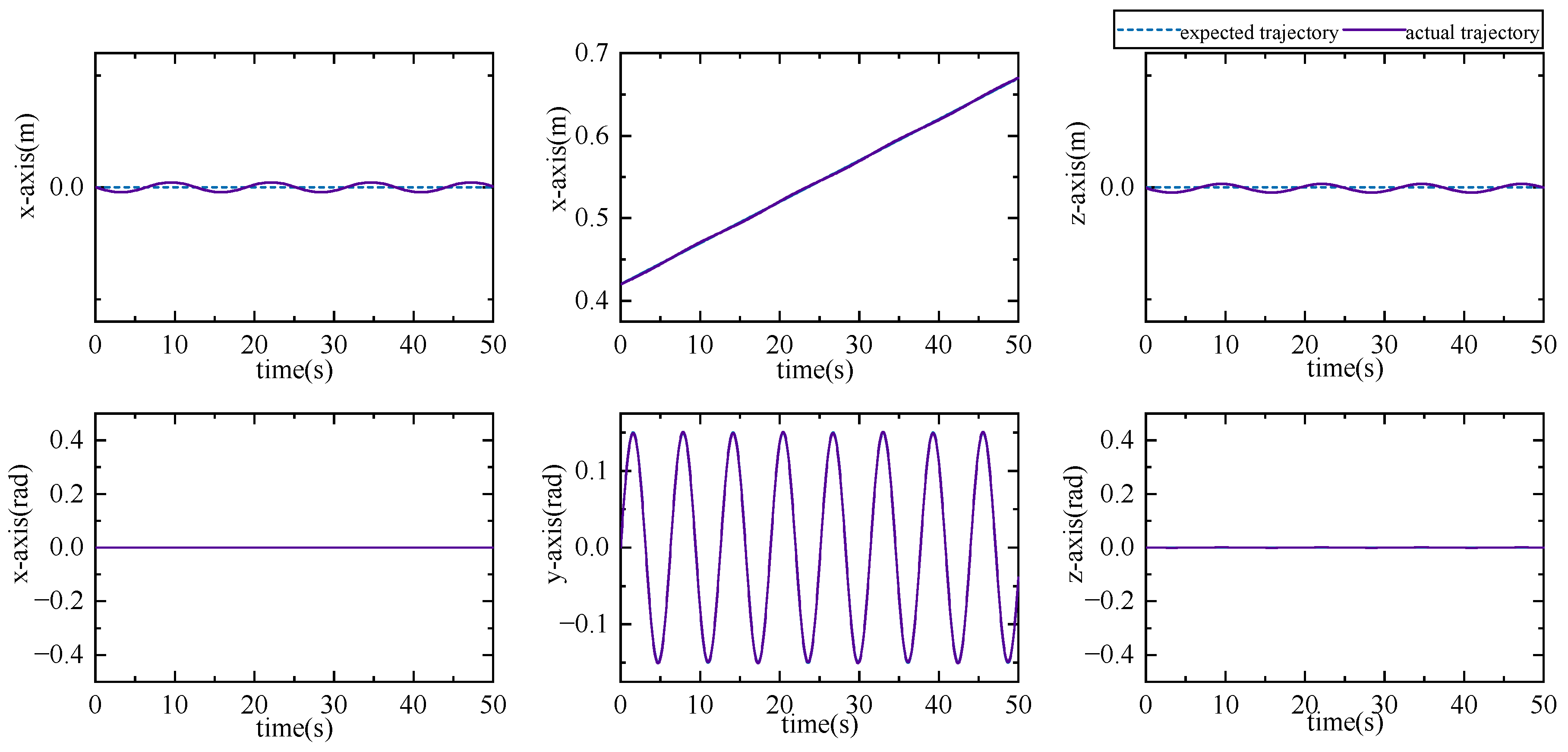
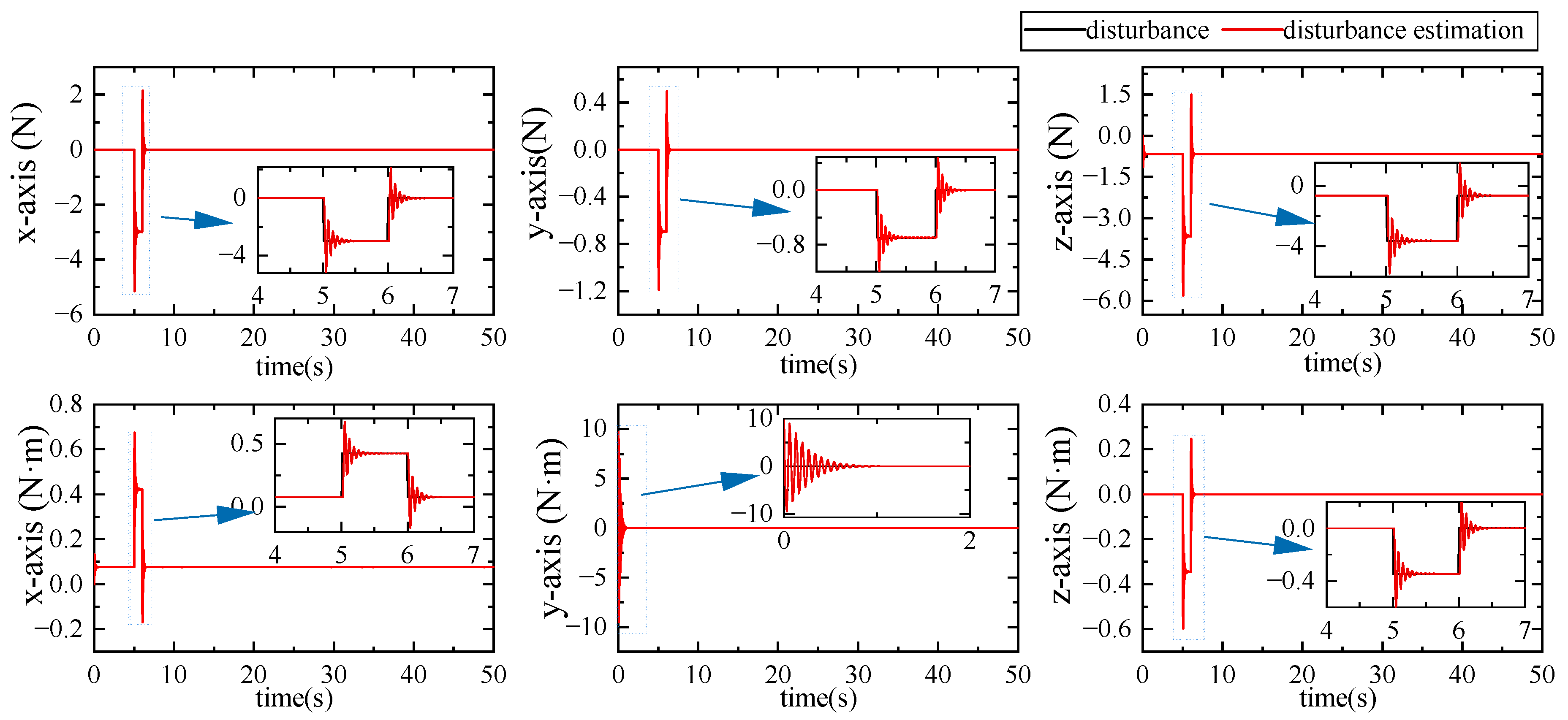
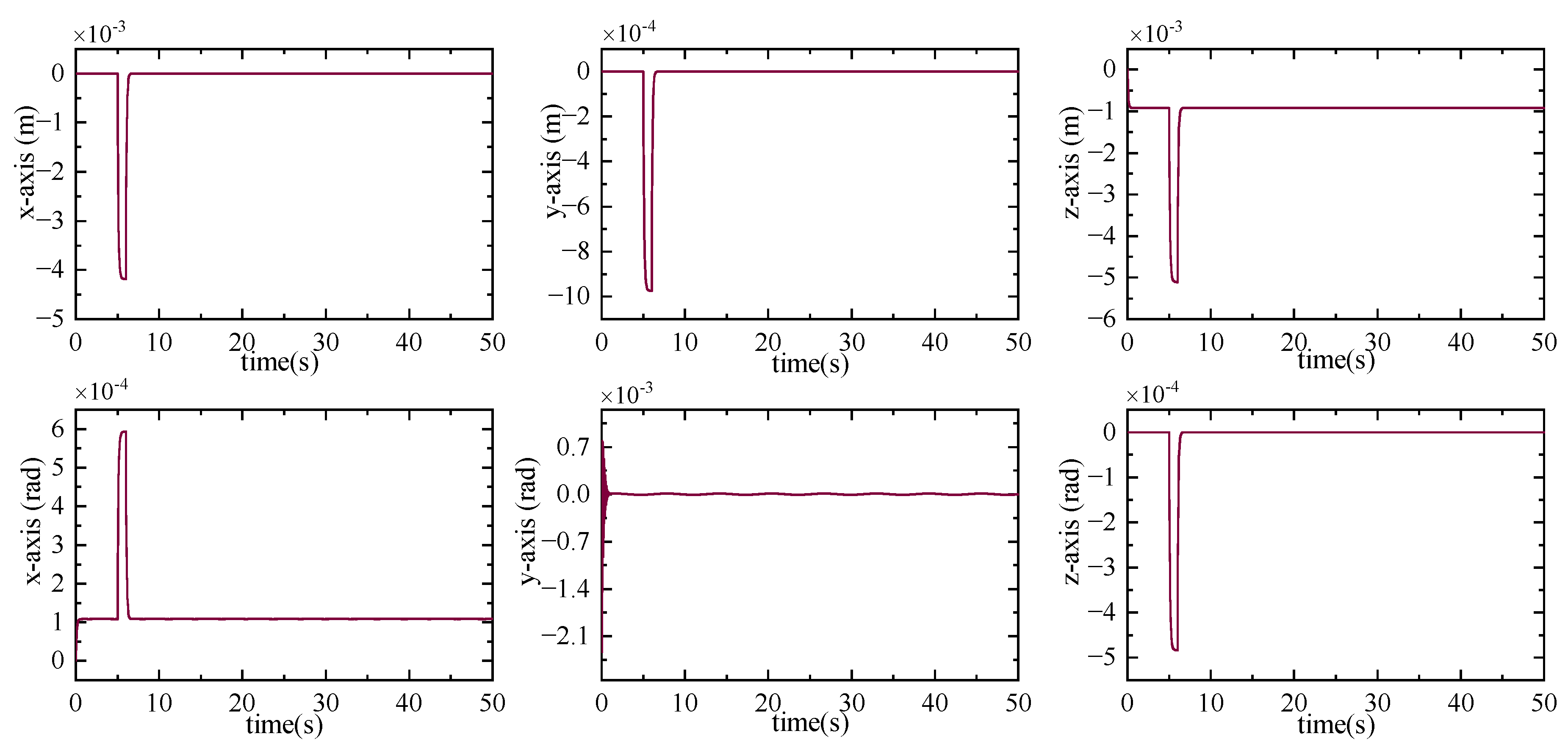
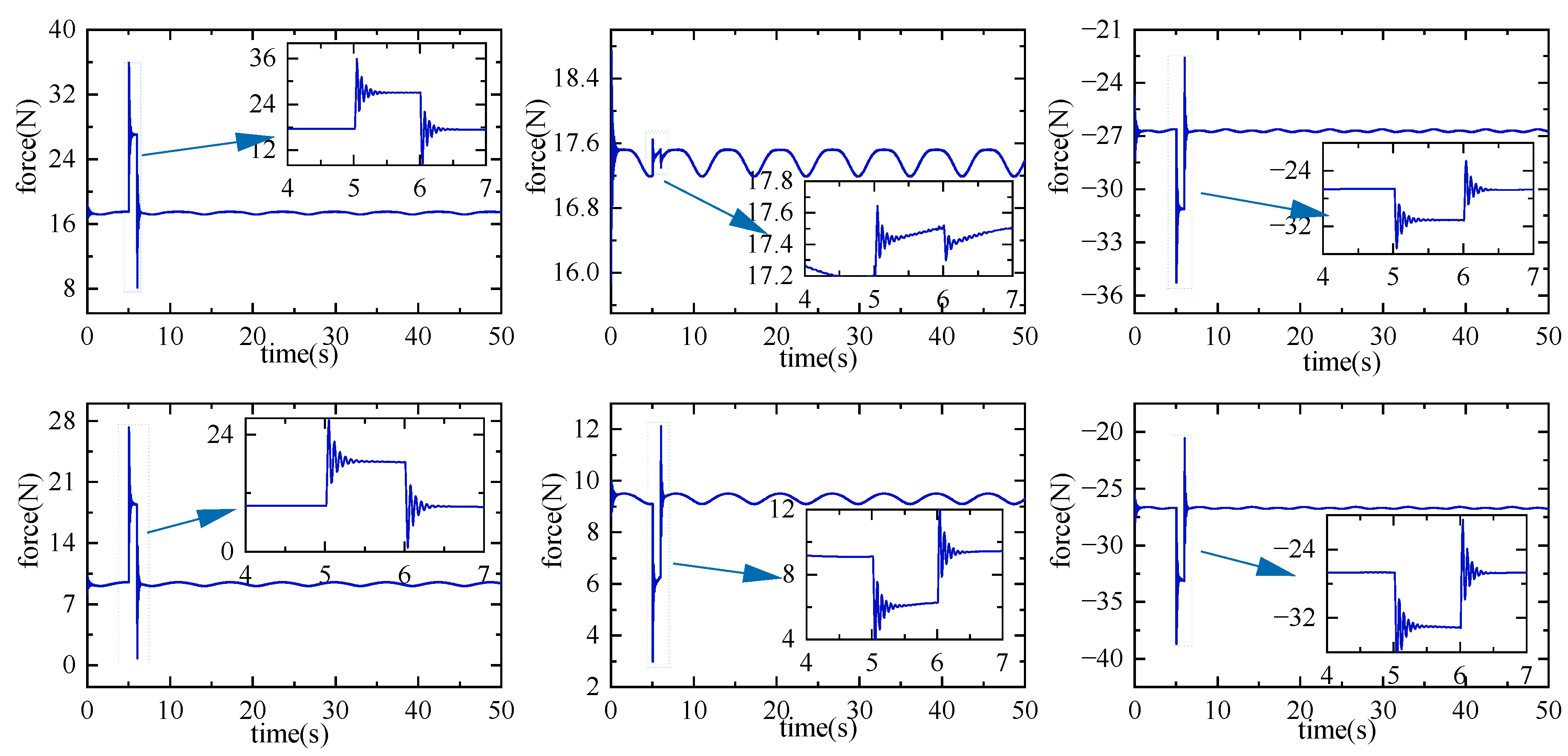
• An improved NFTSM controller is designed, which can effectively cope with the effects of modeling errors and unknown external perturbations. The experimental results show that the error converges to 0 within 0.5 s, realizing high-precision trajectory tracking, and the controller stabilizes the output driving force, which will help to enhance the training effect.

The main elements of the other sections are as follows. Section 2 introduces several typical dynamics derivation methods and robot control strategies and provides a detailed overview of related work on the application of NFTSM control strategies. Section 3 derives the dynamics equations of the 6-PUS parallel mechanism. Section 4 designs the ADE-NFTSM control strategy. Section 5 analyzes the simulation experimental results to verify that the designed control strategy is effective. Section 6 provides conclusions.

2. Problems

Robot dynamics modeling helps in computer simulation, control strategy development, and optimization of physical prototypes [7,8]. Similar to kinematics, dynamics is also divided into two forms. Forward dynamics is the change in the mechanism’s position calculated from the input force or moment of the brake. Inverse dynamics is the calculation of the force or moment of each actuator with a known trajectory of the moving platform [9]. Some typical calculation methods include the Newton–Euler method [10,11,12], the Lagrange method [13,14,15], and the principle of virtual work [16]. Some assumptions are usually needed to simplify the dynamics expressions when applying the Newton–Euler method or the Lagrange method to derive parallel mechanism dynamics, and these methods are less applicable to complex mechanisms. The virtual work principle belongs to the category of dynamic rigid body dynamics modeling strategies, and its equilibrium equations are constructed based on the functional principle in physics. This method ignores the interaction forces between the joints, and only the velocity partial derivatives matrix at a specific point is required for modeling. The complexity of the computational process is significantly lower than that of the Lagrange equations and the Newton–Euler method, and the dynamics model is more uniform from the point of view of the square present of parallel robots with different structures, so this method is more efficient.

The 6-PUS parallel mechanism is a highly nonlinear and highly coupled system with six inputs and six outputs, which has higher coupling and nonlinear characteristics, so it is extremely critical to design an appropriate controller. In previous research, PID control was widely used because of its simple principle and ease of use, but the PID control’s accuracy is not high. The introduction of fuzzy control or other intelligent algorithms can improve the control effect, but the algorithm is completely dependent on experience or requires a lot of training [17,18]. Sliding mode control methods are a class of nonlinear control methods with discontinuous control behavior, in which the system state is made to move along a specified sliding mode surface by switching the control volume. The goal of the control is to make and keep the system state moving on the sliding mode surface. When the system reaches the sliding mode surface, the controller will ensure that the system slides along that surface through feedback control until it reaches the origin of the system, so it is more suitable in a parallel mechanism compared to PID control [19]. Sliding mode control (SMC) is achieved through two phases, one in which the system moves from an arbitrary state to the sliding surface and the other in which it stabilizes on the sliding surface [20]. The conventional SMC has slow convergence and is prone to vibration jitter because the system is not robust during the movement phase towards the sliding surface [21,22]. To solve this problem, some scholars have successively proposed terminal sliding mode control (TSMC) [23] and fast terminal sliding mode control (FTSM) [24], but the controller converges slowly, and the singularity problem occurs, which results in the controller outputting control signals of great amplitude. Non-singular fast terminal sliding mode (NFTSM) control avoids singularity problems [25,26,27,28]. The NFTSM improves the stability and response speed of the system by introducing a non-singularity term and a fast convergence term, which enables the system to converge quickly to the equilibrium state when it is far away from the equilibrium state and, at the same time, converge quickly when it is close to the equilibrium state.

Jyotindra Narayan [29] developed an affordable standing-assisted lower limb exoskeleton for children and proposed the use of a bi-exponential convergence law to improve the NFTSM control scheme. The study shows that the control strategy can converge quickly in finite time and effectively cope with uncertain perturbations and modeling errors. This study can help most children with rehabilitation needs to complete the training. Saleh Mobayen [25] presented an NFTSM control method for underdriven robot arms. The method combines a disturbance observer and SMC to allow the robot to accurately track desired trajectories with good robustness and dynamic performance. The designed controller, under the influence of disturbances, can make the trajectory error converge to 0 within 2.5 s. Emad Oghabi [30] proposed a combination of fuzzy neural network and the NFTSM control method to address the effects of model uncertainty and highly nonlinear external disturbances in cable-driven parallel robots and verified the trajectory tracking capability of the method by numerical simulation, but its cable force fluctuates greatly in the three cables when subjected to disturbances. Liu Q [31] proposed an NFTSM control method based on a nonlinear disturbance observer for a rehabilitation robot for upper limb training that was able to assist patients with elbow and wrist rehabilitation activities. It was experimentally verified that the designed controller enabled the upper limb rehabilitation robot to achieve precise position control, in addition to providing appropriate auxiliary functions. The design of the controller makes the rehabilitation training more compliant and effective. Yi S [32] designed a second-order fast non-singular terminal sliding mode controller. The controller is suitable for robots in the presence of external perturbations and uncertainties and enables trajectory tracking. Experiments show that the drive output is smooth, and the trajectory tracking error converges within 1 s in the presence of disturbances. Lei R [33] enabled the system to achieve fault-tolerant control in finite time, and NFTSM was combined with a dual-power fast approximation law. The improved NFTSM controller can bring the trajectory tracking errors of the spacecraft attitude and robotic arm joints close to 0 within 5 s. The NFTSM controller was also able to control the spacecraft attitude and robotic arm joints with a fast approximation law. Chen J and Zhao C et al. [34] combined disturbance observer and NFTSM control, which uses the disturbance observer to allow the approximation of uncertain external perturbations and counteract the external disturbance, and when the system is in an unknown interference environment, it can ensure the stable operation of the system. Liu C et al. [35] proposed an active disturbance rejection control (ADRC) scheme for the electromagnetic docking of spacecraft. The designed controller can effectively cope with the problems of time lag, external interference, and elliptical eccentricity during the electromagnetic docking of spacecraft. And the designed controller can make the trajectory tracking error reach 10⁻¹⁰ orders of magnitude. Sha L et al. [36,37] proposed NFTSM based on extended state observer (ESO), which can also estimate the disturbance in real time and feed-forward compensation. The disturbance observer and the extended state observer are robust and have high tracking accuracy, but they have strict requirements on the selection of parameters and usually need to solve linear inequalities to calculate the parameters. The dynamics equations of the 6-PUS parallel mechanism studied in this paper and their complexity will make the parameter-solving process more complicated. Lyu B [38] proposed an integrated predictor–observer feedback control strategy for vibration suppression for large spacecraft that combines a state observer, a disturbance observer, and an intermediate observer. The control strategy simultaneously eliminates the effects of unbounded time lags and unknown perturbations on the spacecraft and tracks errors with very high accuracy. However, its design is complex, and the robots studied in this paper do not need to achieve such a high level of accuracy in practical applications. The adoption of this controller may extend the computation time of the system.

Upon comprehensive analysis of the above, some current robot control strategies have high tracking accuracy and no jitter phenomenon. However, there is still room for improvement in the convergence time and stability of the drive under the influence of disturbances. Common anti-disturbance controllers have good control performance but complicated design. In this paper, a non-singular fast terminal sliding mode controller based on adaptive disturbance estimation (ADE-NFTSM) is designed. The NFTSM controller has fast convergence speed, high tracking accuracy, and no jitter phenomenon. The adaptive disturbance estimation strategy estimates the external force applied to the robot according to the position deviation and velocity deviation in the robot motion and performs feed-forward compensation, which has high tracking accuracy and few parameters, and the appropriate parameters can be selected after several experiments. For cerebral palsy patients in the pre-rehabilitation period, the 6-PUS parallel mechanism will be frequently perturbed during rehabilitation due to the lack of balance, which will affect the trajectory of the mechanism. This is the main reason why we designed the ADE-NFTSM controller. The controller designed in this paper has a simple structure, high tracking accuracy, faster convergence time, and more stable output and can effectively handle external perturbations. This controller is designed for cerebral palsy patients who are in the pre-rehabilitation stage, and the 6-PUS parallel mechanism operates stably under the action of the controller to improve the patient’s rehabilitation.

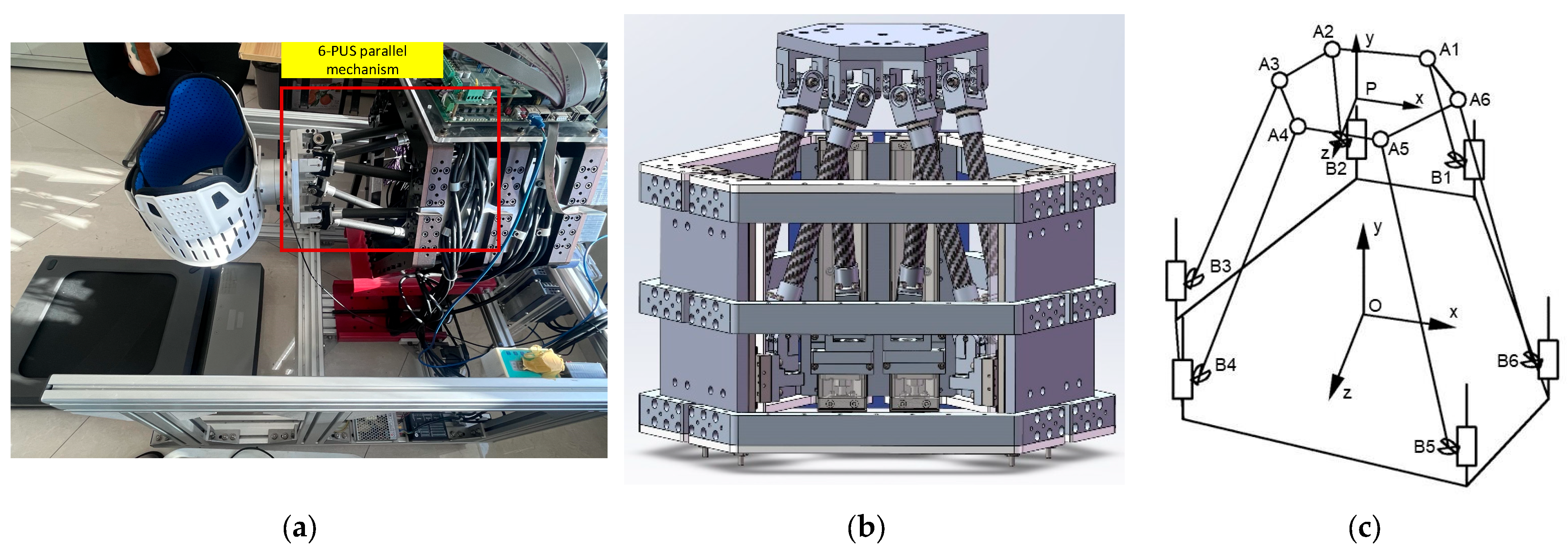
3. Mechanical Dynamics Analysis

Reference [39] analyzes in detail the structure and kinematics of the 6-PUS parallel mechanism. Figure 1a shows the rehabilitation robot for children with cerebral palsy, with the location of where the 6-PUS parallel mechanism is located labeled. The equal scale simulation model of the 6-PUS parallel mechanism is shown in Figure 1b, which is composed of a moving platform, a base, and six links, each of which is connected by a prismatic joint (P), a constant length rod, a universal joint (U), and a spherical joint (S) [39]. Figure 1c shows a sketch of the mechanism where the static coordinate system (O-xyz) and the dynamic coordinate system (P-xyz) are established. The direction of motion of the prismatic joint is the y-axis of the coordinate system (O-xyz).

Table 1. Parameter values when the 6-PUS parallel mechanism is in the initial position.

$\mathit{i}$	${\mathit{x}}_{\mathit{B}\_\mathit{i}}$ (mm)	${\mathit{y}}_{\mathit{B}\_\mathit{i}}$ (mm)	${\mathit{z}}_{\mathit{B}\_\mathit{i}}$ (mm)	${\mathit{x}}_{\mathit{A}\_\mathit{i}}$ (mm)	${\mathit{y}}_{\mathit{A}\_\mathit{i}}$ (mm)	${\mathit{z}}_{\mathit{A}\_\mathit{i}}$ (mm)	$\mathit{l}\_\mathit{i}$ (mm)
1	133.68	−24.99	73.53	61.38	−51.30	420	258.2
2	133.68	24.99	73.53	61.38	51.30	420	258.2
3	−45.19	128.27	73.53	13.74	78.81	420	258.2
4	−88.48	103.27	73.53	−75.12	27.50	420	258.2
5	−88.48	−103.27	73.53	−75.12	−27.50	420	258.2
6	−45.19	−128.27	73.53	13.74	−78.81	420	258.2

shows the parameter values when the 6-PUS parallel mechanism is in the initial position.

From the analysis in the above section, the virtual work principle can avoid the calculation of the constraint force, which calculates the inertia force and moment based on the linear and angular acceleration of the rigid body; the robot is considered to be in equilibrium according to D’Alembert’s principle, and the input forces and moments are solved by the virtual work principle. The robot control process does not need to solve the constraint forces and moments. So, in this paper, the imaginary work principle is used to derive the dynamic equations of the 6-PUS parallel mechanism in the static coordinate system.

3.1. Speed Analysis

The velocities of the 6-PUS parallel mechanism end-movement platforms are as follows:

$$v_P={[{\dot{p}}_x {\dot{p}}_y {\dot{p}}_z]}^{\mathrm{T}}$$

(1)

$${\omega }_P={[\dot{\alpha } \dot{\beta } \dot{\gamma }]}^{\mathrm{T}}$$

(2)

In Equation (1), p_x, p_y, and p_z denote the position of the center point of the moving platform on the three directional axes of the moving coordinate system. $\alpha$, $\beta$, and $\gamma$ in Equation (2) denote the angle of rotation around the three directional axes of the moving coordinate system, respectively.

From Figure 1c, which illustrates the sketch of the mechanism, the vector expression for each connecting rod is as follows:

$$\mathit{P}+\mathit{R}\cdot {\mathit{A}}_i=l{\mathit{e}}_i-{\mathit{B}}_i-{\mathit{y}}_i\hspace{1em}i=1,2,\cdot \cdot \cdot ,6$$

(3)

where $\mathit{R}$ is the rotation matrix, l is the length of the links, and ${\mathit{e}}_i$ is the unit direction vector of the links. Equation (3) is differentiated with respect to time on both the left and right sides, yielding the expression for the linear velocity ${\mathit{v}}_{ai}$ at the center ${\mathit{A}}_i$ of each spherical joint of the moving platform as follows:

$${\mathit{v}}_{ai}={\mathit{v}}_p+{\mathit{\omega }}_p\times {\mathit{a}}_i$$

(4)

$${\mathit{v}}_{ai}={\dot{d}}_i{\mathit{s}}_i+l{\mathit{\omega }}_i\times {\mathit{e}}_i$$

(5)

In Equations (4) and (5), ${\mathit{a}}_i={\mathit{R}}^p{\mathit{a}}_i$ is the coordinates of the position of the spherical joint in the static coordinate system; $d_i$ is the prismatic joint movement length; ${\mathit{s}}_i={[0 0 1]}^{\mathrm{T}}$ is the unit direction vector of the prismatic joint direction of travel.

The prismatic joint velocity and the center of mass of the connecting rod velocity are obtained by dot and fork multiplication ${\mathit{e}}_i$ on both sides of Equation (5), respectively:

$${\dot{d}}_i={\displaystyle \frac{{{\mathit{e}}_i}^{\mathrm{T}}{\mathit{v}}_{ai}}{{{\mathit{e}}_i}^{\mathrm{T}}{\mathit{s}}_i}}$$

(6)

$${\mathit{\omega }}_{li}={\displaystyle \frac{1}{l}}[{\mathit{e}}_i\times {\mathit{v}}_{ai}-{\dot{d}}_i{\mathit{e}}_i\times {\mathit{s}}_i]$$

(7)

The connecting rod velocity is as follows:

$${\mathit{v}}_{li}={\dot{d}}_i{\mathit{s}}_i+{\displaystyle \frac{l}{2}}{\mathit{\omega }}_{li}\times {\mathit{e}}_i$$

(8)

3.2. Acceleration Analysis

The acceleration of the 6-PUS parallel mechanism end-movement platforms are as follows:

$${\dot{v}}_p={[{\ddot{p}}_x {\ddot{p}}_y {\ddot{p}}_z]}^{\mathrm{T}}$$

(9)

$${\dot{\omega }}_p={[\ddot{\alpha } \ddot{\beta } \ddot{\gamma }]}^{\mathrm{T}}$$

(10)

From Equation (4), the acceleration at point ${\mathit{A}}_i$ can also be expressed as follows:

$${\dot{\mathit{v}}}_{ai}={\dot{\mathit{v}}}_p+{\dot{\mathit{\omega }}}_p\times {\mathit{a}}_i+{\mathit{\omega }}_p\times ({\mathit{\omega }}_p\times {\mathit{a}}_i)$$

(11)

Similarly, the acceleration at point ${\mathit{A}}_i$ can also be expressed as follows:

$${\dot{\mathit{v}}}_{ai}={\ddot{d}}_i{\mathit{s}}_i+l{\dot{\mathit{\omega }}}_{li}\times {\mathit{e}}_i+l{\mathit{\omega }}_{li}\times ({\mathit{\omega }}_{li}\times {\mathit{e}}_i)$$

(12)

The prismatic joint acceleration is given by multiplying both sides of Equation (12) by ${\mathit{e}}_i$:

$${\ddot{d}}_i={\displaystyle \frac{{{\mathit{e}}_i}^{\mathrm{T}}{\dot{\mathit{v}}}_{ai}+l{{\mathit{\omega }}_{li}}^{\mathrm{T}}{\mathit{\omega }}_{li}}{{{\mathit{e}}_i}^{\mathrm{T}}{\mathit{s}}_i}}$$

(13)

The angular acceleration of the connecting rod is given by cross-multiplying both sides of Equation (12) by ${\mathit{e}}_i$:

$${\dot{\mathit{\omega }}}_{li}={\displaystyle \frac{1}{l}}[{\mathit{e}}_i\times {\dot{\mathit{v}}}_{ai}-{\displaystyle \frac{{\mathit{e}}_i\times {\mathit{s}}_i}{{{\mathit{e}}_i}^{\mathrm{T}}{\mathit{s}}_i}}({{\mathit{e}}_i}^{\mathrm{T}}{\dot{\mathit{v}}}_{ai}+l{{\mathit{\omega }}_{li}}^{\mathrm{T}}{\mathit{\omega }}_{li})]$$

(14)

From Equation (8), the linear acceleration of the center of mass of the connecting rod is obtained:

$${\dot{\mathit{v}}}_{li}={\ddot{d}}_i{\mathit{s}}_i+{\displaystyle \frac{l}{2}}[{\dot{\mathit{\omega }}}_{li}\times {\mathit{e}}_i+{\mathit{\omega }}_{li}\times ({\mathit{\omega }}_{li}\times {\mathit{e}}_i)]$$

(15)

3.3. Establishment of the Jacobi Matrix

In mathematics, the Jacobi matrix serves to map one vector to another, and it is widely used in various fields. Jacobi matrices are necessary for the dynamics equations to be established in this study. It is necessary to calculate the Jacobi matrices of the brake, the moving sub, and the fixed length linkage with the velocity at the moving platform mass point, respectively.

Let ${\dot{\mathit{x}}}_p={[{\mathit{v}}_p {\mathit{\omega }}_p]}^{\mathrm{T}}$, and Equation (4) can be expressed as follows:

$${\mathit{v}}_{ai}=[{\mathit{I}}_{3\times 3}-{\tilde{\mathit{a}}}_i]{\dot{\mathit{x}}}_p$$

(16)

where ${\mathit{I}}_{3\times 3}$ is the three-dimensional unit matrix, ${\tilde{\mathit{a}}}_i$ is the antisymmetric matrix of ${\mathit{a}}_i$, and similarly, all $\tilde{\Delta }$ appearing below are antisymmetric matrices of $\Delta$.

Let ${\mathit{J}}_{ai}=[{\mathit{I}}_{3\times 3}-{\tilde{\mathit{a}}}_i]$, then the velocity relationship between the endpoints of the moving platform and its center of mass is as follows:

$${\mathit{v}}_{ai}={\mathit{J}}_{ai}{\dot{\mathit{x}}}_p$$

(17)

Let ${\mathit{J}}_{inv\_i}={\displaystyle \frac{{{\mathit{e}}_i}^{\mathrm{T}}}{{{\mathit{e}}_i}^{\mathrm{T}}{\mathit{s}}_i}}{\mathit{J}}_{ai}$, and Equation (6) can be written as follows:

$$\dot{d}={\mathit{J}}_{inv}{\dot{\mathit{x}}}_p$$

(18)

where ${\mathit{J}}_{inv}={[{\mathit{J}}_{inv\_1} \cdots {\mathit{J}}_{inv\_6}]}^{\mathrm{T}}$, and ${\mathit{J}}_{inv}$ is the Jacobi matrix of velocities between the brake and the center point of the 6-PUS parallel mechanism end-movement platforms.

The prismatic joint velocity is given by Equation (5):

$${\mathit{v}}_{bi}={\mathit{s}}_i{\dot{d}}_i$$

(19)

The prismatic joint is confined to the track, and it can only perform translational motion and cannot perform rotational motion. Therefore, ${\mathit{\omega }}_{bi}={[0 0 0]}^{\mathrm{T}}$. The Jacobi matrix of velocity between the individual prismatic joint and the center of the 6-PUS parallel mechanism end-movement platforms can be obtained as follows:

$${\mathit{J}}_{bi}=\left[\begin{array}{c}{\mathit{s}}_i{\mathit{J}}_{inv\_i}\\ 0_{3\ast 6}\end{array}\right]$$

(20)

Based on the Equations (7), (17), and (19), connecting rod angular acceleration is obtained:

$${\mathit{\omega }}_{li}={\displaystyle \frac{1}{l}}[{\tilde{\mathit{e}}}_i{\mathit{J}}_{ai}-({\mathit{e}}_i\times {\mathit{s}}_i){\mathit{J}}_{inv}]{\dot{\mathit{x}}}_p$$

(21)

According to the equation of linear velocity of connecting rod calculated by Equation (8), the following equation is obtained by substituting Equations (17) and (18):

$${\mathit{v}}_{li}=[({\mathit{s}}_i+{\displaystyle \frac{1}{2}}{\tilde{\mathit{e}}}_i({\mathit{e}}_i\times {\mathit{s}}_i)){\mathit{J}}_{inv}-{\displaystyle \frac{1}{2}}{\tilde{\mathit{e}}}_i{\tilde{\mathit{e}}}_i{\mathit{J}}_{ai}]{\dot{\mathit{x}}}_p$$

(22)

Let ${\mathit{J}}_{\omega li}={\displaystyle \frac{1}{l}}[{\tilde{\mathit{e}}}_i{\mathit{J}}_{ai}-({\mathit{e}}_i\times {\mathit{s}}_i){\mathit{J}}_{inv}]$, ${\mathit{J}}_{vli}=[({\mathit{s}}_i+{\displaystyle \frac{1}{2}}{\tilde{\mathit{e}}}_i({\mathit{e}}_i\times {\mathit{s}}_i)){\mathit{J}}_{inv}-{\displaystyle \frac{1}{2}}{\tilde{\mathit{e}}}_i{\tilde{\mathit{e}}}_i{\mathit{J}}_{ai}]$. Then:

$${\dot{\mathit{x}}}_{li}=\left[\begin{array}{c}{\mathit{J}}_{vli}\\ {\mathit{J}}_{\omega li}\end{array}\right]{\dot{\mathit{x}}}_p$$

(23)

Let ${\mathit{J}}_{li}=\left[\begin{array}{c}{\mathit{J}}_{vli}\\ {\mathit{J}}_{\omega li}\end{array}\right]$, and ${\mathit{J}}_{li}$ is the Jacobi matrix between the linkage and the moving platform.

3.4. Establishment of Dynamics Equations

From the principle of virtual work, the work done by the generalized active force and the generalized inertial force at each joint of the 6-PUS parallel mechanism is 0. The generalized active and inertial combined forces ${\mathit{F}}_p$, ${\mathit{F}}_{bi}$, and ${\mathit{F}}_{li}$ on the center of mass of the moving platform, the center of mass of the prismatic joints, and the center of mass of the links are expressed in the stationary system, respectively, as follows:

$${\mathit{F}}_p=\left[\begin{array}{c}{\mathit{f}}_p\\ {\mathit{n}}_p\end{array}\right]=\left[\begin{array}{c}{\mathit{f}}_e+m_p\mathit{g}-m_p{\dot{\mathit{v}}}_p\\ {\mathit{n}}_e-{}^o\mathit{I}{}_p\dot{\mathit{\omega }}_p-{\mathit{\omega }}_p\times ({}^o\mathit{I}{}_p\mathit{\omega }_p)\end{array}\right]$$

(24)

$${\mathit{F}}_{bi}=\left[\begin{array}{c}{\mathit{f}}_{bi}\\ {\mathit{n}}_{bi}\end{array}\right]=\left[\begin{array}{c}{m}_b\mathit{g}-m_b{\dot{\mathit{v}}}_{bi}\\ 0\end{array}\right]$$

(25)

$${\mathit{F}}_{li}=\left[\begin{array}{c}{\mathit{f}}_{li}\\ {\mathit{n}}_{li}\end{array}\right]=\left[\begin{array}{c}{m}_l\mathit{g}-m_l{\dot{\mathit{v}}}_{li}\\ -{}^o\mathit{I}{}_{li}\dot{\mathit{\omega }}_{li}-{\mathit{\omega }}_{li}\times ({}^o\mathit{I}{}_{li}\omega _{li})\end{array}\right]$$

(26)

In Equations (24)–(26), p, b, and l denote the 6-PUS parallel mechanism end-movement platforms, the prismatic joint, and the link, respectively. $\mathit{f}$ is the force vector, and $\mathit{n}$ is the moment vector; ${\mathit{f}}_e$ and ${\mathit{n}}_e$ are the force and moment acting on the moving platform, respectively; $\mathit{v}$, $\mathit{\omega }$ represent the linear and angular velocities of the joint, respectively; $\dot{\mathit{v}}$, $\dot{\mathit{\omega }}$ represent the linear and angular acceleration of the joint; ${}^o\mathit{I}$ represents the moment of inertia of the joint around its center of mass in the static coordinate system, $\mathit{m}$ is the mass of the joint, and $\mathit{g}$ is the gravitational acceleration vector.

The dynamics equation of the 6-PUS parallel mechanism is derived from the principle of virtual work:

$$\mathit{\tau }=-{{\mathit{J}}_{inv}}^{-\mathrm{T}}[{\mathit{F}}_p+{\displaystyle \sum _{i=1}^6{{\mathit{J}}_{bi}}^{\mathrm{T}}{\mathit{F}}_{bi}}+{\displaystyle \sum _{i=1}^6{{\mathit{J}}_{li}}^{\mathrm{T}}{\mathit{F}}_{li}}]$$

(27)

where ${\mathit{J}}_{inv}$, ${\mathit{J}}_{bi}$, and ${\mathit{J}}_{li}$ are the Jacobi matrix derived in the above section.

Write Equation (27) as a standard form:

$$\mathit{M}(\mathit{x})\ddot{\mathit{x}}+\mathit{C}(\mathit{x},\dot{\mathit{x}})\dot{\mathit{x}}+\mathit{G}(\mathit{x})=-{{\mathit{J}}_{inv}}^T\mathit{\tau }+{\mathit{F}}_{ext}$$

(28)

where x is the vector of the moving platform $\mathit{x}={[P_x P_y P_z \alpha \beta \gamma ]}^{\mathrm{T}}$, $\mathit{M}(\mathit{x})\ddot{\mathit{x}}$ is the inertial force term, $\mathit{C}(\mathit{x},\dot{\mathit{x}})\dot{\mathit{x}}$ is the centripetal and Coriolis force term, $\mathit{G}(\mathit{x})$ is the gravity term, and ${\mathit{F}}_{ext}$ is an uncertain external force acting on the end of a 6-PUS parallel mechanism.

4. Research on Non-Singular Fast Terminal Sliding Mode Control Strategy Based on Adaptive Disturbance Estimation

This section details the design and stability proof of ADE-NFTSM control strategy. In practice, considering the modeling error of the 6-PUS parallel mechanism and the unknown external perturbations, the mechanism dynamical equations is expressed as follows:

$$({\mathit{M}}_0+\Delta \mathit{M})\ddot{\mathit{x}}+({\mathit{C}}_0+\Delta \mathit{C})\dot{\mathit{x}}+({\mathit{G}}_0+\Delta \mathit{G})=-{{\mathit{J}}_{inv}}^{\mathrm{T}}\mathit{\tau }+{\mathit{F}}_{\mathit{e}\mathit{x}\mathit{t}}$$

(29)

where ${\mathit{M}}_0$, ${\mathit{C}}_0$, and ${\mathit{G}}_0$ are the nominal inertial force term, the centripetal and Coriolis force term, and the gravity term, respectively; $\Delta \mathit{M}$, $\Delta \mathit{C}$, and $\Delta \mathit{G}$ are the modeling errors corresponding to each part of the dynamical model, respectively, so that the dynamical model of the real system is as follows:

$$\ddot{\mathit{x}}={{\mathit{M}}_0}^{-1}(-{{\mathit{J}}_{inv}}^{\mathrm{T}}\mathit{\tau }-{\mathit{C}}_0\dot{\mathit{x}}-{\mathit{G}}_0)+\Delta \mathit{q}$$

(30)

$$\Delta \mathit{q}={{\mathit{M}}_0}^{-1}({\mathit{F}}_{\mathit{e}\mathit{x}\mathit{t}}-\Delta \mathit{M}\ddot{\mathit{x}}-\Delta \mathit{C}\dot{\mathit{x}}-\Delta \mathit{G})$$

(31)

where $\Delta \mathit{q}$ is the sum of modeling uncertainties and disturbance uncertainties.

The 6-PUS parallel mechanism has a complex structure. To enable it to achieve high-accuracy trajectory tracking in the presence of complex disturbances, this paper designs an ADE-NFTSM control strategy. The designed controller expression is complex. In order to simplify the expression form, the following symbolic representation is quoted to be applied in this article:

$$sig{(\mathit{a})}^b={[{\left|a_1\right|}^{b_1}sign(a_1),{\left|a_2\right|}^{b_2}sign(a_2),\cdot \cdot \cdot ,{\left|a_n\right|}^{b_n}sign(a_n)]}^{\mathrm{T}}$$

(32)

$${\left|\mathit{a}\right|}^b={[{\left|a_1\right|}^{b_1},{\left|a_2\right|}^{b_2},\cdot \cdot \cdot ,{\left|a_n\right|}^{b_n}]}^{\mathrm{T}}$$

(33)

$${\mathit{a}}^{\mathit{b}}={[{a_1}^{b_1},{a_2}^{b_2},\cdot \cdot \cdot ,{a_n}^{b_n}]}^{\mathrm{T}}$$

(34)

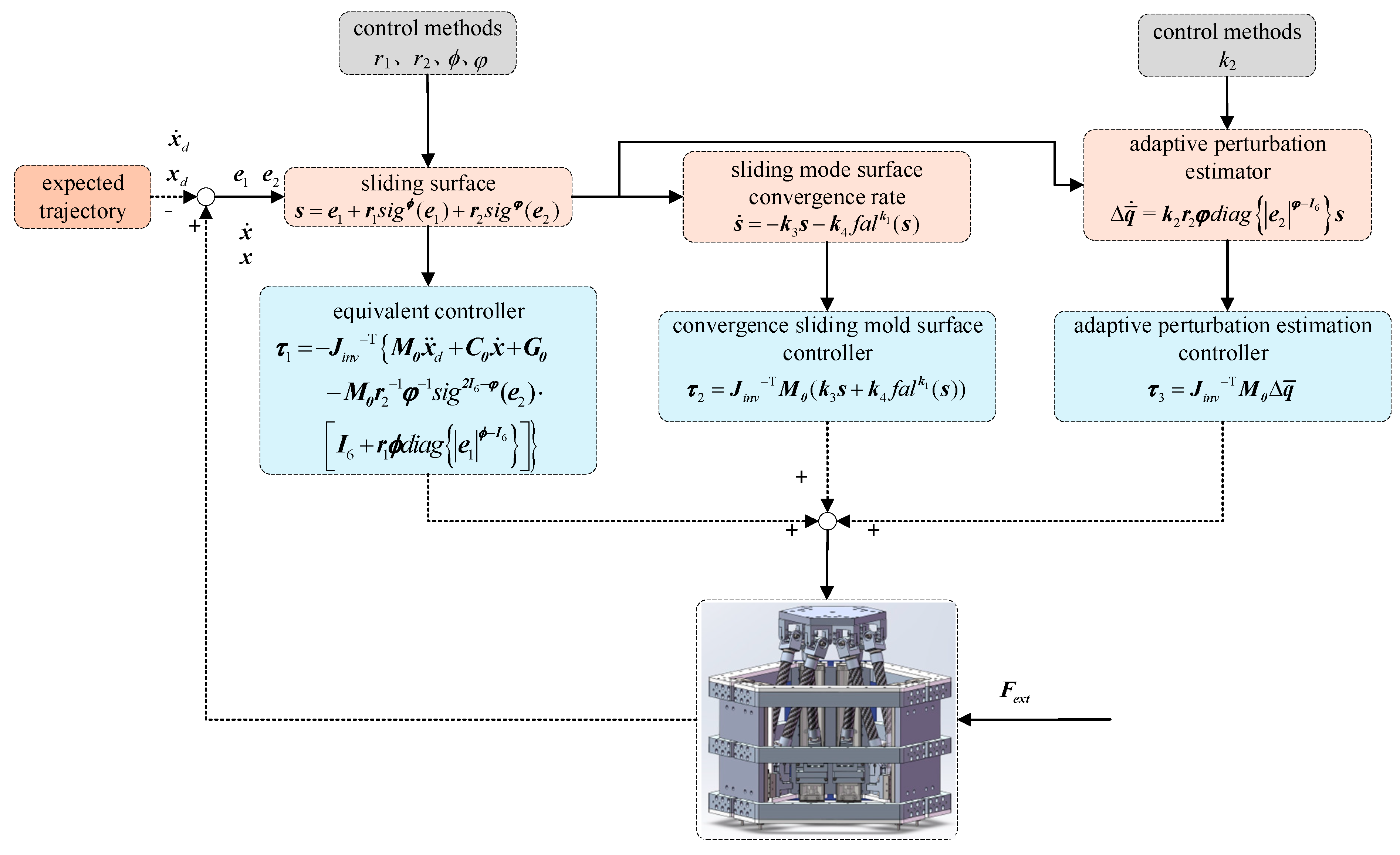
4.1. Controller Design

Define ${\mathit{x}}_d$, ${\dot{\mathit{x}}}_d$ as the ideal position and ideal speed of motion of the mechanism. The error of the 6-PUS parallel mechanism in trajectory tracking is expressed as follows:

$$\left\{\begin{array}{c}{\mathit{e}}_1=\mathit{x}-{\mathit{x}}_d\\ {\mathit{e}}_2=\dot{\mathit{x}}-{\dot{\mathit{x}}}_d\end{array}\right.$$

(35)

Considering a 6-PUS parallel mechanism with complex structure and many joints, we have analyzed and compared a variety of sliding mode functions. Finally, this paper chooses the following sliding surface:

$$\mathit{s}={\mathit{e}}_1+{\mathit{r}}_{1}si{g}^{\mathit{\varphi }}\left({\mathit{e}}_1\right)+{\mathit{r}}_{2}si{g}^{\mathit{\phi }}\left({\mathit{e}}_2\right)$$

(36)

where ${\varphi }_i>{\phi }_i$, $1<{\phi }_i<2$, ${\mathit{r}}_{1i}>0$, ${\mathit{r}}_{2i}>0$, $i=1,2,\cdot \cdot \cdot ,6$, (all occurrences of i in the article indicate this range of values) ${\mathit{r}}_1=diag\left\{r_{11},r_{12},\cdot \cdot \cdot ,r_{16}\right\}$, ${\mathit{r}}_2=diag\left\{r_{11},r_{12},\cdot \cdot \cdot ,r_{16}\right\}$, $\mathit{\varphi }=diag\left\{{\varphi }_{21},{\varphi }_{22},\cdot \cdot \cdot ,{\varphi }_{26}\right\}$, and $\mathit{\phi }=diag\left\{{\phi }_{21},{\phi }_{22},\cdot \cdot \cdot ,{\phi }_{26}\right\}$. When the robotic system is moving on the sliding surface, $\mathit{s}=0$, and then Equation (36) can be written as follows:

$${\mathit{e}}_2=-{[{{\mathit{r}}_2}^{-1}{\mathit{e}}_1+{{\mathit{r}}_2}^{-1}{\mathit{r}}_{1}si{g}^{\mathit{\varphi }}({\mathit{e}}_1\left)\right]}^{1/\mathit{\phi }}$$

(37)

When the system status is not close to the equilibrium point, i.e., ${\mathit{e}}_{1i}>1$ or ${\mathit{e}}_{1i}<-1$, at this time, the convergence time is mainly dominated by the higher-order term in the sliding surface $\mathit{s}$. So, the sliding mode surface $\mathit{s}$ can be expressed as $\mathit{s}={\mathit{e}}_1+{\mathit{r}}_{1}si{g}^{\mathit{\varphi }}\left({\mathit{e}}_1\right)$. Currently, ${\mathit{e}}_2=-{[{{\mathit{r}}_2}^{-1}{\mathit{r}}_{1}si{g}^{\mathit{\varphi }}({\mathit{e}}_1\left)\right]}^{1/\mathit{\phi }}$, and because $\mathit{\varphi }/\mathit{\phi }>1$, state variables have a larger convergence rate. When the system status is near the equilibrium point, i.e., $-1<{\mathit{e}}_{1i}<1$, the higher-order term $si{g}^{\mathit{\varphi }}\left({\mathit{e}}_1\right)$ in the sliding surface can be neglected, at which point the sliding surface is $\mathit{s}={\mathit{e}}_1+{\mathit{r}}_{2}si{g}^{\mathit{\phi }}\left({\mathit{e}}_2\right)$, ${\mathit{e}}_2=-{[{{\mathit{r}}_2}^{-1}{\mathit{e}}_1]}^{1/\mathit{\phi }}$; because $1/\mathit{\phi }<1$, the system has a faster convergence rate. Therefore, the use of non-singular fast terminal sliding surface ensures the system converges in a finite time in any case of non-zero ${\mathit{e}}_1$, ${\mathit{e}}_2$. The following proof of controller stability also verifies this feature of the sliding surface.

Equation (36) is derived as follows:

$$\left\{\begin{array}{c}{\displaystyle \frac{d}{dt}}(si{g}^{\mathit{\varphi }}({\mathit{e}}_1))=\mathit{\varphi }diag\left\{{\left|{\mathit{e}}_1\right|}^{\mathit{\varphi }-{\mathit{I}}_6}\right\}{\dot{\mathit{e}}}_1\\ {\displaystyle \frac{d}{dt}}(si{g}^{\mathit{\phi }}({\mathit{e}}_2))=\mathit{\phi }diag\left\{{\left|{\mathit{e}}_2\right|}^{\mathit{\phi }-{\mathit{I}}_6}\right\}{\dot{\mathit{e}}}_2\end{array}\right.$$

(38)

$$\dot{\mathit{s}}={\dot{\mathit{e}}}_1+{\mathit{r}}_1\mathit{\varphi }diag\left\{{\left|{\mathit{e}}_1\right|}^{\mathit{\varphi }-{\mathit{I}}_6}\right\}{\dot{\mathit{e}}}_1+{\mathit{r}}_2\mathit{\phi }diag\left\{{\left|{\mathit{e}}_2\right|}^{\mathit{\phi }-{\mathit{I}}_6}\right\}{\dot{\mathit{e}}}_2$$

(39)

From Equations (29) and (35), the acceleration tracking error of 6-PUS parallel mechanism end platforms is as follows:

$${\dot{\mathit{e}}}_2=\ddot{\mathit{x}}-{\ddot{\mathit{x}}}_d={{\mathit{M}}_0}^{-1}(-{{\mathit{J}}_{inv}}^{\mathrm{T}}\mathit{\tau }-{\mathit{C}}_0\dot{\mathit{x}}-{\mathit{G}}_0-{\mathit{M}}_0{\ddot{\mathit{x}}}_d)+\Delta \mathit{q}$$

(40)

The next step after selecting a suitable sliding surface is to design the equivalent controller. The equivalent controller allows the system’s state trajectory to produce equivalent motion on sliding surface, and $\dot{\mathit{s}}=0$ is a necessary condition. Substituting Equation (40) into Equation (39) and letting $\dot{\mathit{s}}=0$ results in the equivalent controller ${\tau }_1$, with the expression as follows:

$${\mathit{\tau }}_1=-{{\mathit{J}}_{inv}}^{-\mathrm{T}}\left\{{\mathit{M}}_0{\ddot{\mathit{x}}}_d+{\mathit{C}}_0\dot{\mathit{x}}+{\mathit{G}}_0-{\mathit{M}}_0{{\mathit{r}}_2}^{-1}{\mathit{\phi }}^{-1}si{g}^{2{\mathit{I}}_6-\mathit{\phi }}\left({\mathit{e}}_2\right)\left[{\mathit{I}}_6+{\mathit{r}}_1\mathit{\varphi }diag\left\{{\left|{\mathit{e}}_1\right|}^{\mathit{\varphi }-{\mathit{I}}_6}\right\}\right]\right\}$$

(41)

In the case where each parameter is known and there is no disturbance, ${\mathit{\tau }}_1$ makes the system move on the slide surface. To meet the needs of the existence of modeling errors and external unknown disturbance in practice, the convergent sliding mode controller ${\mathit{\tau }}_2$ is designed, which enables the system to move onto the slide mode surface in finite time but does not produce an equivalent sliding mode motion. The convergence rate of the designed sliding surface is as follows:

$$\dot{\mathit{s}}=-{\mathit{k}}_3\mathit{s}-{\mathit{k}}_{4}fa{l}^{{\mathit{k}}_1}(\mathit{s})$$

(42)

To make ${\mathit{e}}_1$, ${\mathit{e}}_2$ converge to the origin of the sliding surface, here, the controller selects the power function $fal(a)$, $fal(a)=\left\{\begin{array}{ll}{\left|a\right|}^{{\delta }_1}sign(a),& \left|a\right|>{\delta }_2\\ a/{{\delta }_2}^{1-{\delta }_1},& \left|a\right|\le {\delta }_2\end{array}\right.$; ${\delta }_1$ and ${\delta }_2$ are all designable constant-value parameters. $0<{\delta }_1<1$, $0<{\delta }_2<1$, ${\mathit{k}}_1=diag\{k_{11},k_{12},\cdot \cdot \cdot ,k_{16}\}$, ${\mathit{k}}_3=diag\{k_{31},k_{32},\cdot \cdot \cdot ,k_{36}\}$, ${\mathit{k}}_4=diag\{k_{41},k_{42},\cdot \cdot \cdot ,k_{46}\}$, $0<{\mathit{k}}_1<1$, ${\mathit{k}}_3>0$, ${\mathit{k}}_4>0$, $fal{(\mathit{a})}^b={[{\left|a_1\right|}^{b_1}fal(a_1),{\left|a_2\right|}^{b_2}fal(a_2),\cdot \cdot \cdot ,{\left|a_n\right|}^{b_n}fal(a_n)]}^{\mathrm{T}}=diag\{fal(\mathit{a})\}{\left|\mathit{a}\right|}^{\mathit{b}}$.

The convergent sliding mode controller expression is as follows:

$${\mathit{\tau }}_2={{\mathit{J}}_{inv}}^{-\mathrm{T}}{\mathit{M}}_0({\mathit{k}}_3\mathit{s}+{\mathit{k}}_{4}fa{l}^{{\mathit{k}}_1}(\mathit{s}))$$

(43)

The external disturbance may vary greatly in magnitude, large or small, and are highly uncertain. In order to allow the system to achieve more accurate control, this external disturbance needs to be canceled out. And with the use of the equipment due to wear and tear and other reasons, mechanical connections will have gaps, leading to a decrease in the control results. The two control strategies devised above are based on the ideal situation, and in this regard, it is the design of the adaptive disturbance estimation strategy ${\tau }_3$. The control strategy ${\tau }_3$ is used to estimate the disturbances acting at the end of the 6-PUS parallel mechanism and neutralize the disturbances acting at the end of the 6-PUS parallel mechanism through feed-forward compensation. By adding the adaptive disturbance estimation strategy, the robotic system can minimize its actual trajectory error, bringing it close to 0. The expression of the controller is as follows:

$${\mathit{\tau }}_3={{\mathit{J}}_{inv}}^{-T}{\mathit{M}}_0\Delta \overline{\mathit{q}}$$

(44)

$$\Delta \dot{\overline{\mathit{q}}}={\mathit{k}}_2{\mathit{r}}_2\mathit{\phi }diag\left\{{\left|{\mathit{e}}_2\right|}^{\mathit{\phi }-{\mathit{I}}_6}\right\}\mathit{s}$$

(45)

where $\Delta \overline{\mathit{q}}$ is the adaptive disturbance estimation term; ${\mathit{k}}_2=diag\{{\mathit{k}}_{21},{\mathit{k}}_{22},\cdot \cdot \cdot ,{\mathit{k}}_{26}\}$, ${\mathit{k}}_2>0$.

So, the overall controller design is as follows:

$$\begin{array}{ll}\hfill \mathit{\tau }=& {\mathit{\tau }}_1+{\mathit{\tau }}_2+{\mathit{\tau }}_3\\ \hfill =& -{{\mathit{J}}_{inv}}^{-\mathrm{T}}\left\{{\mathit{M}}_0{\ddot{\mathit{x}}}_d+{\mathit{C}}_0\dot{\mathit{x}}+{\mathit{G}}_0-{\mathit{M}}_0{{\mathit{r}}_2}^{-1}{\mathit{\phi }}^{-1}si{g}^{2{\mathit{I}}_6-\mathit{\phi }}\left({\mathit{e}}_2\right)\left[{\mathit{I}}_6+{\mathit{r}}_1\mathit{\varphi }diag\left\{{\left|{\mathit{e}}_1\right|}^{\mathit{\varphi }-{\mathit{I}}_6}\right\}\right]\right.\\ & \left.-{\mathit{M}}_0({\mathit{k}}_3\mathit{s}+{\mathit{k}}_{4}fa{l}^{{\mathit{k}}_1}(\mathit{s}))-{\mathit{M}}_0\Delta \overline{\mathit{q}}\right\}\end{array}$$

(46)

Figure 2 shows the overall framework of the designed controller:

The ADE-NFTSM controller converges quickly and has the advantages of high control accuracy and no jitter. Under the action of the total controller, the motion trajectory of the robot system will approach the desired trajectory. While under the action of the adaptive disturbance estimation strategy, the motion trajectory will converge asymptotically:

$$\dot{\mathit{s}}=0\hspace{1em}{\mathit{e}}_1=0\hspace{1em}{\mathit{e}}_2=0$$

Substituting Equation (46) into the robot dynamics Equation (10), the closed-loop equation is as follows:

$${\dot{\mathit{e}}}_2=-{{\mathit{r}}_2}^{-1}{\mathit{\phi }}^{-1}si{g}^{2{\mathit{I}}_6-\mathit{\phi }}\left({\mathit{e}}_2\right)\left[{\mathit{I}}_6+{\mathit{r}}_1\mathit{\varphi }diag\left\{{\left|{\mathit{e}}_1\right|}^{\mathit{\varphi }-{\mathit{I}}_6}\right\}\right]-{\mathit{k}}_3\mathit{s}-{\mathit{k}}_{4}fa{l}^{{\mathit{k}}_1}(\mathit{s})-\Delta \stackrel{⌢}{\mathit{q}}$$

(47)

where $\Delta \stackrel{⌢}{\mathit{q}}=\Delta \overline{\mathit{q}}-\Delta \mathit{q}$.

4.2. Proof of Stability of the Controller

Lemma 1.

Suppose there exists a Lyapunov function $V(x)$, with initial value $V(t_0)$ satisfied:

$$\dot{V}(x)\le -\alpha V(x)-\beta V^{\gamma }(x)$$

where   $\alpha$ and   $\beta$ are two positive scalars, and   $0<\gamma <1$. Thus, for any initial time t₀ the Lyapunov function converges in finite time to   $V(x)=0$, with a convergence time T:

$$T=t_0+{\displaystyle \frac{1}{\alpha (1-\gamma )}}\ln {\displaystyle \frac{\alpha V^{1-\rho }(t_0)+\beta }{\beta }}$$

Get:

$$\mathrm{T}\le {\displaystyle \frac{1}{\alpha (1-\gamma )}}\ln {\displaystyle \frac{\alpha V^{1-\rho }(t_0)+\beta }{\beta }}$$

The Lyapunov function is $\mathit{V}={\displaystyle \frac{1}{2}}{\mathit{s}}^{\mathrm{T}}\mathit{s}$, for which the derivative and substitution of Equation (39) gives the following:

$$\dot{\mathit{V}}={\displaystyle \frac{1}{2}}{\mathit{s}}^{\mathrm{T}}[{\dot{\mathit{e}}}_1+{\mathit{r}}_1\mathit{\varphi }diag\left\{{\left|{\mathit{e}}_1\right|}^{\mathit{\varphi }-{\mathit{I}}_6}\right\}{\dot{\mathit{e}}}_1+{\mathit{r}}_2\mathit{\phi }diag\left\{{\left|{\mathit{e}}_2\right|}^{\mathit{\phi }-{\mathit{I}}_6}\right\}{\dot{\mathit{e}}}_2]$$

(48)

Substitute Equations (30), (35), and (46) into Equation (48):

$$\dot{\mathit{V}}=-{\mathit{s}}^{\mathrm{T}}{\mathit{r}}_2\mathit{\phi }diag\left\{{\left|{\mathit{e}}_2\right|}^{\mathit{\phi }-{\mathit{I}}_6}\right\}[{\mathit{k}}_3\mathit{s}+{\mathit{k}}_{4}fa{l}^{{\mathit{k}}_1}(\mathit{s})+\Delta \stackrel{⌢}{\mathit{q}}]$$

(49)

Equation (49) can be written as the following two expressions:

$${\dot{\mathit{V}}}_a=-{\mathit{s}}^{\mathrm{T}}{\mathit{r}}_2\mathit{\phi }diag\left\{{\left|{\mathit{e}}_2\right|}^{\mathit{\phi }-{\mathit{I}}_6}\right\}\left[[{\mathit{k}}_3+diag\{\Delta \stackrel{⌢}{\mathit{q}}\left\}dia{g}^{-1}\right\{s\}]\mathit{s}+{\mathit{k}}_{4}fa{l}^{{\mathit{k}}_1}(\mathit{s})\right]$$

(50)

$${\dot{\mathit{V}}}_{\mathit{b}}=-{\mathit{s}}^{\mathrm{T}}{\mathit{r}}_2\mathit{\phi }diag\left\{{\left|{\mathit{e}}_2\right|}^{\mathit{\phi }-{\mathit{I}}_6}\right\}\left[{\mathit{k}}_3\mathit{s}+[{\mathit{k}}_4+diag\{\Delta \stackrel{⌢}{\mathit{q}}\left\}dia{g}^{-1}\right\{fa{l}^{{\mathit{k}}_1}(\mathit{s})\}]fa{l}^{{\mathit{k}}_1}(\mathit{s})\right]$$

(51)

For Equation (50), let ${\xi }_1={\mathit{r}}_2\mathit{\phi }diag\left\{{\left|{\mathit{e}}_2\right|}^{\mathit{\phi }-{\mathit{I}}_6}\right\}[{\mathit{k}}_3+diag\{\Delta \stackrel{⌢}{\mathit{q}}\left\}dia{g}^{-1}\right\{s\}]$, ${\mathit{\xi }}_2={\mathit{r}}_2\mathit{\phi }diag\left\{{\left|{\mathit{e}}_2\right|}^{\mathit{\phi }-{\mathit{I}}_6}\right\}{\mathit{k}}_4$, ${\mathit{\xi }}_3={\mathit{\xi }}_{2}diag\left\{\left|fal(\mathit{s})\right|\right\}$. Then, Equation (50) can be written as follows:

$${\dot{\mathit{V}}}_a=-{\mathit{s}}^{\mathrm{T}}{\mathit{\xi }}_1\mathit{s}-{\left|\mathit{s}\right|}^{\mathrm{T}}{\mathit{\xi }}_3{\left|\mathit{s}\right|}^{{\mathit{k}}_1}$$

(52)

Substitute $\mathit{V}={\displaystyle \frac{1}{2}}{\mathit{s}}^{\mathrm{T}}\mathit{s}$ into Equation (52):

$${\dot{\mathit{V}}}_a=-2{\mathit{\xi }}_1\mathit{V}-2^{({\mathit{k}}_1+1)/2}{\mathit{\xi }}_3{\mathit{V}}^{({\mathit{k}}_1+1)/2}$$

(53)

Consider ${\mathit{e}}_2\ne 0$. Assuming that ${\mathit{\xi }}_1>0$, ${\mathit{\xi }}_2>0$, ${\mathit{\xi }}_3>0$, then by Lemma 1, the convergence time of ${\mathit{V}}_a$ is as follows:

$$T\le {\displaystyle \frac{1}{{\mathit{\xi }}_1(1-{\mathit{k}}_1)}}ln{\displaystyle \frac{2{\mathit{\xi }}_1{\mathit{V}}^{(1-{\mathit{k}}_1)/2}(t_0)+2^{(1+{\mathit{k}}_1)/2}{\mathit{\xi }}_3}{2^{(1+{\mathit{k}}_1)/2}{\mathit{\xi }}_3}}$$

(54)

By the definition of ${\mathit{\xi }}_2$ and ${\mathit{\xi }}_3$, it can be seen that they are always more than 0. In order to satisfy ${\mathit{\xi }}_1>0$, the following is necessary:

$${\mathit{k}}_3+diag\{\Delta \stackrel{⌢}{\mathit{q}}\}dia{g}^{-1}\left\{s\right\}>0$$

(55)

It is known that ${\mathit{k}}_3>0$, and if $diag\{\Delta \stackrel{⌢}{\mathit{q}}\}dia{g}^{-1}\left\{s\right\}>0$, then Equation (55) is greater than 0; if $diag\{\Delta \stackrel{⌢}{\mathit{q}}\}dia{g}^{-1}\left\{s\right\}<0$ is obtained:

$${\mathit{k}}_3>diag\left\{\left|\Delta \stackrel{⌢}{\mathit{q}}\right|\right\}dia{g}^{-1}\left\{\left|s\right|\right\}$$

(56)

So:

$$\left|s\right|>{{\mathit{k}}_3}^{-1}\left|\Delta \stackrel{⌢}{\mathit{q}}\right|$$

(57)

Thus, s will converge in finite time to: $\left|s\right|\le {{\mathit{k}}_3}^{-1}\left|\Delta \stackrel{⌢}{\mathit{q}}\right|={\mathit{d}}_1$.

When ${\mathit{e}}_2=0$, derivation of ${\mathit{e}}_2$ and substitution of Equation (47) yields the following:

$$\Delta \stackrel{⌢}{\mathit{q}}=-{\mathit{k}}_3\mathit{s}-{\mathit{k}}_{4}fa{l}^{{\mathit{k}}_1}(\mathit{s})-{\dot{\mathit{e}}}_2$$

(58)

In the region $\left|s\right|>{\mathit{d}}_1$, $s>0$ yields $\left|\Delta \stackrel{⌢}{\mathit{q}}\right|<{\mathit{k}}_{3}s$, i.e., $-{\mathit{k}}_{3}s<\Delta \stackrel{⌢}{\mathit{q}}<{\mathit{k}}_{3}s$. Substituting Equation (58) yields the following:

$$-2{\mathit{k}}_{3}s-{\mathit{k}}_{4}fa{l}^{{\mathit{k}}_1}(\mathit{s})<{\dot{\mathit{e}}}_2<-{\mathit{k}}_{4}fa{l}^{{\mathit{k}}_1}(\mathit{s})$$

(59)

At this point, ${\dot{\mathit{e}}}_2<0$ if $s<0$ yields $\left|\Delta \stackrel{⌢}{\mathit{q}}\right|<-{\mathit{k}}_{3}s$, i.e., ${\mathit{k}}_{3}s<\Delta \stackrel{⌢}{\mathit{q}}<-{\mathit{k}}_{3}s$. Substituting Equation (58) yields the following:

$$-{\mathit{k}}_{4}fa{l}^{{\mathit{k}}_1}(\mathit{s})<{\dot{\mathit{e}}}_2<-2{\mathit{k}}_{3}s-{\mathit{k}}_{4}fa{l}^{{\mathit{k}}_1}(\mathit{s})$$

(60)

At this point, ${\dot{\mathit{e}}}_2>0$. Combining these analyses when ${\mathit{e}}_2=0$, ${\dot{\mathit{e}}}_2>0$, or ${\dot{\mathit{e}}}_2<0$, the system will not stay in the state of ${\mathit{e}}_2=0$.

Analyzing Equation (51) in the same way, s will converge into $\left|s\right|\le {\left[{{\mathit{k}}_4}^{-1}\left|\Delta \stackrel{⌢}{\mathit{q}}\right|\right]}^{1/k1}={\mathit{d}}_2$ in finite time. Thus, s will converge in finite time to $\left|s\right|\le \mathit{d}=min\{{\mathit{d}}_1,{\mathit{d}}_2\}$.

Next, it is shown that the system converges under the action of the disturbance estimation $\Delta \overline{\mathit{q}}$. The Lyapunov function is chosen:

$${\mathit{V}}^{\prime }={\displaystyle \frac{1}{2}}{\mathit{s}}^{\mathrm{T}}\mathit{s}+{\displaystyle \frac{1}{2}}{{\mathit{k}}_4}^{-1}{\left|\Delta \stackrel{⌢}{\mathit{q}}\right|}^2$$

(61)

$${\dot{\mathit{V}}}^{\prime }=-{\mathit{s}}^{\mathrm{T}}{\mathit{r}}_2\mathit{\phi }diag\left\{{\left|{\mathit{e}}_2\right|}^{\mathit{\phi }-{\mathit{I}}_6}\right\}[{\mathit{k}}_3\mathit{s}+{\mathit{k}}_{4}fa{l}^{{\mathit{k}}_1}(\mathit{s})+\Delta \stackrel{⌢}{\mathit{q}}]+{{\mathit{k}}_4}^{-1}\Delta \dot{\overline{\mathit{q}}}\Delta \stackrel{⌢}{\mathit{q}}$$

(62)

Substitute Equation (50):

$${\dot{\mathit{V}}}^{\prime }=-{\mathit{s}}^{\mathrm{T}}{\mathit{r}}_2\mathit{\phi }diag\left\{{\left|{\mathit{e}}_2\right|}^{\mathit{\phi }-{\mathit{I}}_6}\right\}[{\mathit{k}}_3\mathit{s}+{\mathit{k}}_{4}fa{l}^{{\mathit{k}}_1}(\mathit{s})]\le 0$$

(63)

So, the designed controller is stable.

5. Experiments

The dynamics derivation and controller design of the 6-PUS parallel mechanism were completed in the above section, and the main content of this section is to conduct simulation experiments on the theoretical model derived to verify its correctness. The experiments include dynamics simulation experiments and controller simulation experiments.

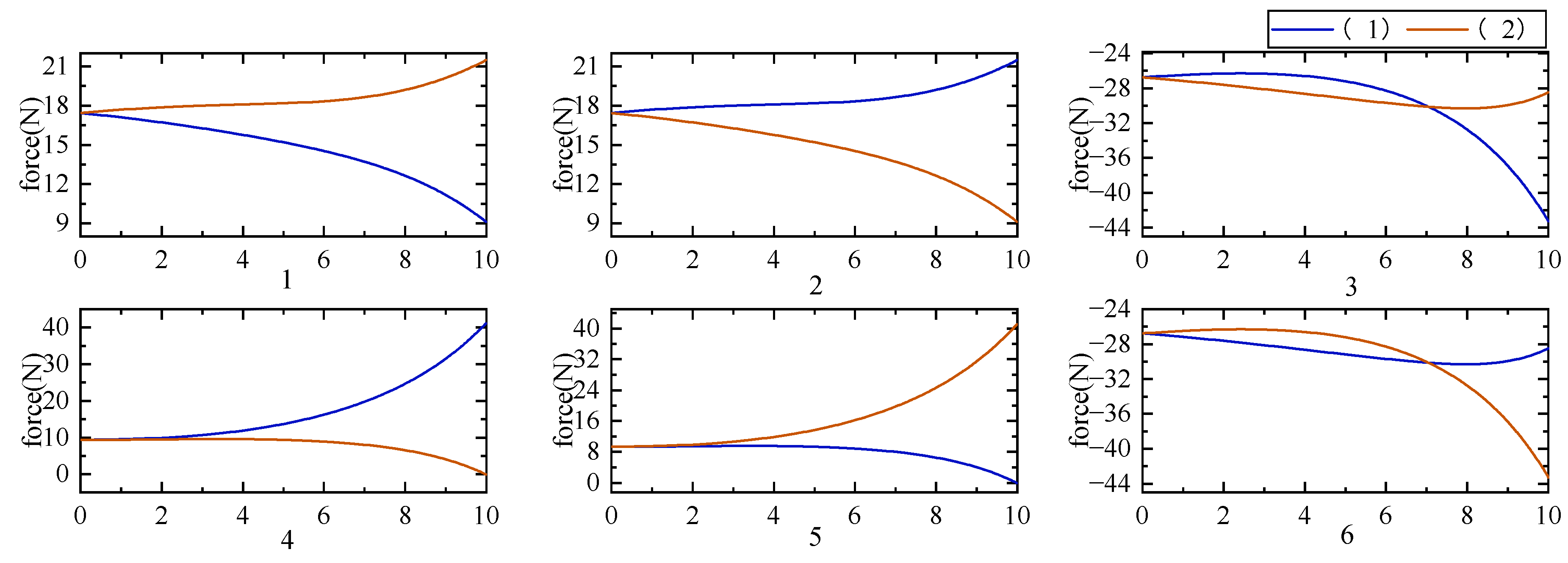
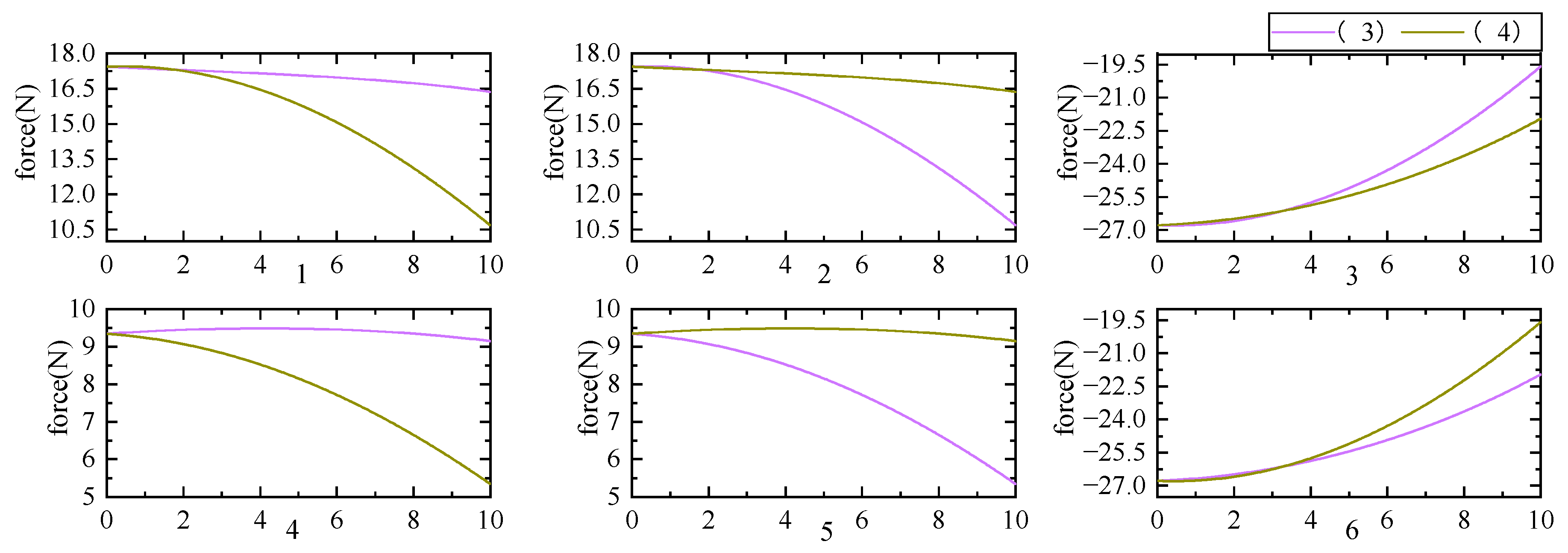
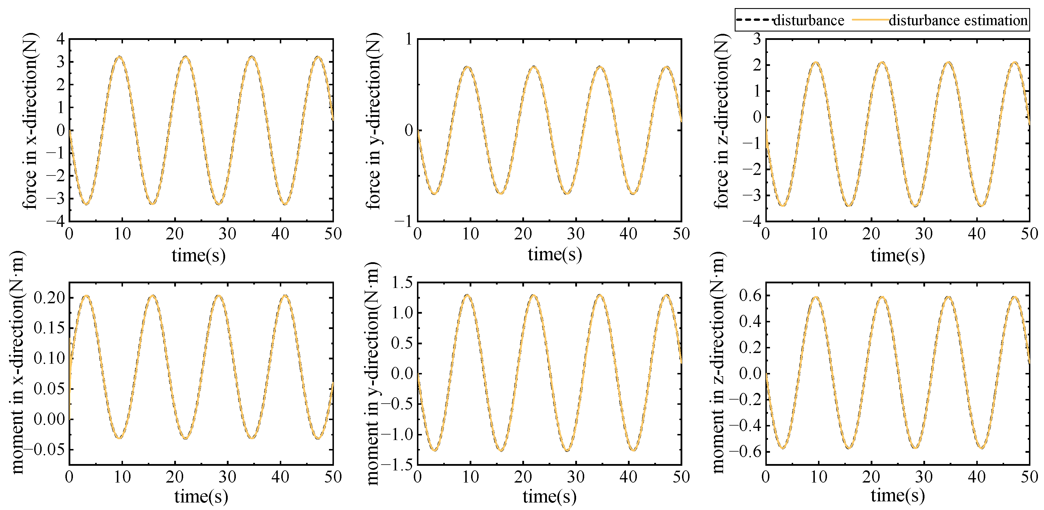
5.1. Dynamics Numerical Simulation Experiment

In this part, the above-deduced dynamics formula is written as a program in MATLAB 2019 for dynamics simulation verification, assuming that the mechanism is analyzed under the action of gravity without adding other external forces and moments, and the gravitational acceleration g = [0 0 − 9.087]^T m/s². According to the simulation capabilities provided by the SolidWorks 2022 software from Dassault Systemes, the relevant parameters used in obtaining the equations include m_p = 1.734 kg, m_b = 0.719 kg, m_l = 0.171 kg, and l = 0.2582 m. According to the dimensions of each component, the moment of inertia of the end platform and the fixed-length linkage of the 6-PUS parallel mechanism are as follows:

$${}^p\mathit{I}_p=\left[\begin{array}{ccc}3.486& 0& 0\\ 0& 6.620& 0\\ 0& 0& 3.486\end{array}\right]\cdot {10}^{-3}\mathrm{kg}\cdot {\mathrm{m}}^2 {}^{Bi}\mathit{I}_{li}=\left[\begin{array}{ccc}0.8& 0& 0\\ 0& 0.2& 0\\ 0& 0& 0.8\end{array}\right]\cdot {10}^{-3}\mathrm{kg}\cdot {\mathrm{m}}^2$$

The dynamics are analyzed in two cases. In the first case, the moving platform is kept constant, and the moving platform makes rotational motions as follows:

(1) x = [0 0.42 0 0 −0.1t −0.1t]^T

(2) x = [0 0.42 0 0 0.1t 0.1t]^T

According to the design characteristics of the 6-PUS parallel mechanism, when the mechanism performs rotary motion around the y-axis and z-axis in opposite directions, the driving force of motors 1 and 2, 3 and 6, and 4 and 5 have symmetry. Figure 3 shows the variation curves of the driving force with time when the motor is doing the two motions (1) and (2), and it can be seen that the variation curves of the driving force with time satisfy the symmetry.

The second case lets the moving platform move without rotational motion and lets its center of mass move according to the following two trajectories:

(3) x = [−0.008t 0.42 0.008t 0 0 0]^T

(4) x = [0.008t 0.42 0.008t 0 0 0]^T

According to the characteristics of the mechanism, when the 6-PUS parallel mechanism end platform center of mass performs translational motion along the x-axis and z-axis, the driving force of the motors should satisfy the symmetry. It can be seen from Figure 4 that when performing the two symmetrical motions of (3) and (4), the motors 1 and 2, 3 and 6, and 4 and 5 satisfy the symmetry. Simulation results show that the dynamical equations of the mechanism are modeled correctly.

5.2. Controller Simulation Experiment

The controller was designed above and proved its stability, and the following further verifies the performances of the ADE-NFTSM controller in MATLAB 2019/Simulink from MathWorks Inc, Natick, MA, USA.

Designing the desired trajectory:

$$\begin{array}{l}{\mathit{x}}_d={[0 0.42+0.05t 0 0 0.15\sin (t) 0]}^{\mathrm{T}}\\ {\dot{\mathit{x}}}_d={[0 0.05 0 0 0.15\cos (t) 0]}^{\mathrm{T}}\\ {\ddot{\mathit{x}}}_d={[0 0 0 0 -0.15\sin (t) 0]}^{\mathrm{T}}\end{array}$$

The initial position and velocity of the center of mass of the platform at the end of the 6-PUS parallel mechanism are ${\mathit{x}}_d={[0 0.42 0 0 0 0]}^{\mathrm{T}}$ and ${\dot{\mathit{x}}}_d={[0 0.05 0 0 0.15 0]}^{\mathrm{T}}$, respectively; the modeling errors are $\Delta \mathit{M}=5\%\times \mathit{M}$, $\Delta \mathit{C}=5\%\times \mathit{C}$, and $\Delta \mathit{G}=5\%\times \mathit{G}$. The parameters of controller ${\tau }_1$ are selected as follows:

$${\mathit{r}}_1=diag\left\{1.5,1.5,1.5,1.5,1.5,1.5\right\}$$

$${\mathit{r}}_2=diag\left\{0.09,0.09,0.09,0.09,0.09,0.09\right\}$$

$$\varphi =diag\left\{2,2,2,2,2,2\right\}$$

$$\phi =diag\left\{1.001,1.001,1.001,1.001,1.001,1.001\right\}$$

The parameters of controller ${\tau }_2$ are selected as follows:

$${\mathit{k}}_1=diag\{0.5,0.5,0.5,0.5,0.5,0.5\}$$

$${\mathit{k}}_3=diag\{1,1,1,1,1,1\}$$

$${\mathit{k}}_4=diag\{1,1,1,1,1,1\}$$

The parameters of the control strategy ${\tau }_3$ are designed as ${\mathit{k}}_2=diag\{8,8,8,8,8,8\}\times {10}^5$, the length of the simulation experiment is 50 s, and sampling is every 0.01 s. The parameters such as mass, inertia tensor, and links’ length of 6-PUS parallel mechanism required in the control simulation experiments have been listed in the previous chapter. The external disturbance cannot be predicted in practical applications, so special attention should be paid to the controller’s estimation of the disturbance in the control simulation experiments, conducting two experiments to validate the effectiveness of the adaptive disturbance estimation strategy. In the first case, the external disturbance changes smoothly, and the disturbance expression is as follows:

$${\mathit{F}}_{\mathit{e}\mathit{x}\mathit{t}}={[5\sin (0.5t) 5\sin (0.5t) 5\sin (0.5t) 0.1\sin (0.5t) 0.1\sin (0.5t) 0.1\sin (0.5t)]}^{\mathrm{T}}\mathrm{N}$$

According to the above control simulation results, from Figure 5, the adaptive disturbance estimation strategy can approximate the external disturbance very well, so that the error of the input 6-PUS parallel mechanism is controlled within a very small range; shown in Figure 6 and Figure 7, when the external disturbance acts smoothly on the system, the ADE-NFTSM controller has a better trajectory tracking ability, and the accuracy of trajectory tracking is very high. The designed motion trajectory of the 6-PUS parallel mechanism is almost perfectly matched with the ideal trajectory, where the maximum positional error is 0.0045 m, and the maximum angular error is 0.001 rad. In summary, even if there are modeling errors and external unknown disturbances in the robotic system, the designed controller is still able to achieve the tracking of the ideal trajectory of the robot very well and control the error within a very small range. From Figure 8, the designed controller has a small fluctuation at the beginning of the motion, but it tends to stabilize in a very short time, and no further fluctuation occurs after stabilization, which keeps the 6-PUS parallel mechanism in a stable state of operation.

The second case is that the system is suddenly perturbed during motion. The other parameters are the same as the first simulation experiment, and the experimental design applies a step signal with amplitude 5 N at 5–6 s of the system motion with the following expression:

$${\mathit{F}}_{\mathit{e}\mathit{x}\mathit{t}}={[5 5 5 0 0 0]}^{\mathrm{T}}\mathrm{N}\hspace{1em}(5\mathrm{s}<t<6\mathrm{s})$$

From Figure 9, Figure 10, Figure 11 and Figure 12, even if the system is suddenly perturbed during the motion, the controller can still control the system motion well. From Figure 12, when the system is running smoothly, the adaptive disturbance estimation strategy can accurately approximate the external perturbation; when the system is suddenly perturbed, there is a small fluctuation in the disturbance estimation term, but the disturbance estimation tends to stabilize and has a high approximation accuracy within 0.5 s. In Figure 10, which shows the comparison between the ideal trajectory and the actual trajectory, the adaptive disturbance estimation strategy can ensure that the system operates under the ideal trajectory. At 5–6 s, there is a small degree of deviation between the ideal trajectory and the actual trajectory. However, Figure 11 shows the ideal trajectory and the actual trajectory error graph, where the maximum position error is 4 mm, and the maximum angular error is 0.006 rad, which meets the robot system’s requirements for accuracy. As seen in Figure 12, when the system is suddenly subjected to external perturbation, the controller can also maintain stable output as a whole; similar to the adaptive disturbance estimation strategy, the controller output will have a small fluctuation at the moment of being perturbed and disappearing of the perturbation, but it tends to stabilize within 0.5 s.

6. Conclusions

In this paper, the trajectory-tracking function of a robot is realized by using dynamics. Firstly, the dynamics formulation of the mechanism is analyzed. Secondly, the advantages and disadvantages of different sliding mode controllers are compared and analyzed, and then the NFTSM control program is chosen, which has fast convergence, high control accuracy, and vibration shaking phenomenon. Finally, considering the existence of external perturbations and dynamics modeling errors during the robot’s motion, an adaptive disturbance estimation strategy is proposed for feed-forward compensation.

The above simulation experiments show that the derived dynamics formula is correct, and the NFTSM controller designed by the dynamic formula has good performance. Moreover, with the adaptive disturbance estimation strategy, whether the external perturbation is smoothly applied to the system or suddenly applied to the system, the designed controller can allow the system to run along the ideal trajectory well. This ensures stable system operation, which, in turn, improves patient rehabilitation. The next step is to further carry out algorithm testing experiments on top of the rehabilitation robot based on simulation analysis to verify the applicability of the algorithm.

References

1. Patel, P.; Baier, J.; Baranov, E.; Khurana, E.; Gambrah-Sampaney, C.; Johnson, A.; Monokwane, B.; Bearden, D.R. Health beliefs regarding pediatric cerebral palsy among caregivers in Botswana: A qualitative study. Child Care Health Dev. 2017, 43, 861–868. [Google Scholar] [CrossRef]
2. Zanon, M.A.; Pacheco, R.L.; Latorraca, C.d.O.C.; Martimbianco, A.L.C.; Pachito, D.V.; Riera, R. Neurodevelopmental Treatment (Bobath) for Children With Cerebral Palsy: A Systematic Review. J. Child Neurol. 2019, 34, 679–686. [Google Scholar] [CrossRef] [PubMed]
3. Sakzewski, L.; Ziviani, J.; Boyd, R.N. Delivering Evidence-Based Upper Limb Rehabilitation for Children with Cerebral Palsy: Barriers and Enablers Identified by Three Pediatric Teams. Phys. Occup. Ther. Pediatr. 2013, 34, 368–383. [Google Scholar] [CrossRef] [PubMed]
4. DiFazio, R.L.; Vessey, J.A.; Miller, P.E.; Snyder, B.D.; Shore, B.J. Health-related quality of life and caregiver burden after hip reconstruction and spinal fusion in children with spastic cerebral palsy. Dev. Med. Child Neurol. 2021, 64, 80–87. [Google Scholar] [CrossRef] [PubMed]
5. Shea, J.; Nunally, K.D.; Miller, P.E.; Difazio, R.; Matheney, T.H.; Snyder, B.; Shore, B.J. Hip Reconstruction in Nonambulatory Children With Cerebral Palsy: Identifying Risk Factors Associated With Postoperative Complications and Prolonged Length of Stay. J. Pediatr. Orthop. 2020, 40, e972–e977. [Google Scholar] [CrossRef]
6. Shore, B.J.; Shrader, M.W.; Narayanan, U.; Miller, F.; Graham, H.K.; Mulpuri, K. Hip Surveillance for Children With Cerebral Palsy: A Survey of the POSNA Membership. J. Pediatr. Orthop. 2017, 37, e409–e414. [Google Scholar] [CrossRef]
7. Tsai, L.-W. Solving the Inverse Dynamics of a Stewart-Gough Manipulator by the Principle of Virtual Work. J. Mech. Des. 2000, 122, 3–9. [Google Scholar] [CrossRef]
8. Mejri, S.; Gagnol, V.; Le, T.-P.; Sabourin, L.; Ray, P.; Paultre, P. Dynamic characterization of machining robot and stability analysis. Int. J. Adv. Manuf. Technol. 2015, 82, 351–359. [Google Scholar] [CrossRef]
9. Pappalardo, C.M.; Guida, D. Forward and Inverse Dynamics of a Unicycle-Like Mobile Robot. Machines 2019, 7, 5. [Google Scholar] [CrossRef]
10. Hess-Coelho, T.A.; Orsino, R.M.M.; Malvezzi, F. Modular modelling methodology applied to the dynamic analysis of parallel mechanisms. Mech. Mach. Theory 2021, 161, 104332. [Google Scholar] [CrossRef]
11. Kunquan, L.; Rui, W. Closed-form Dynamic Equations of the 6-RSS Parallel Mechanism through the Newton-Euler Approach. In Proceedings of the 2011 Third International Conference on Measuring Technology and Mechatronics Automation, Shangshai, China, 6–7 January 2011; pp. 712–715. [Google Scholar]
12. Bascetta, L.; Ferretti, G.; Scaglioni, B. Closed form Newton–Euler dynamic model of flexible manipulators. Robotica 2015, 35, 1006–1030. [Google Scholar] [CrossRef]
13. Staicu, S.; Zhang, D. A novel dynamic modelling approach for parallel mechanisms analysis. Robot. Comput.-Integr. Manuf. 2008, 24, 167–172. [Google Scholar] [CrossRef]
14. Li, Q.; Li, B.; Zhao, X. Dynamic Analysis of a New Type of Asymmetrical Parallel Mechanism Based on Lagrange Method. IOP Conf. Ser. Mater. Sci. Eng. 2018, 428, 012074. [Google Scholar] [CrossRef]
15. Abdellatif, H.; Heimann, B. Computational efficient inverse dynamics of 6-DOF fully parallel manipulators by using the Lagrangian formalism. Mech. Mach. Theory 2009, 44, 192–207. [Google Scholar] [CrossRef]
16. Pedrammehr, S.; Nahavandi, S.; Abdi, H. Closed-form dynamics of a hexarot parallel manipulator by means of the principle of virtual work. Acta Mech. Sin. 2018, 34, 883–895. [Google Scholar] [CrossRef]
17. Tan, X.Q.; Li, G.Y. NN-PID Adaptive Control for 6_PUS Parallel Mechanism. Appl. Mech. Mater. 2012, 226–228, 636–640. [Google Scholar] [CrossRef]
18. Shukla, A.; Karki, H. Modeling simulation & control of 6-DOF Parallel Manipulator using PID controller and compensator. IFAC Proc. Vol. 2014, 47, 421–428. [Google Scholar]
19. Vo, A.T.; Kang, H.-J. A Novel Fault-Tolerant Control Method for Robot Manipulators Based on Non-Singular Fast Terminal Sliding Mode Control and Disturbance Observer. IEEE Access 2020, 8, 109388–109400. [Google Scholar] [CrossRef]
20. Mobayen, S.; Tchier, F. A novel robust adaptive second-order sliding mode tracking control technique for uncertain dynamical systems with matched and unmatched disturbances. Int. J. Control Autom. Syst. 2017, 15, 1097–1106. [Google Scholar] [CrossRef]
21. El Fadili, Y.; Berrada, Y.; Boumhidi, I. Improved sliding mode control law for wind power systems. Int. J. Dyn. Control 2024, 12, 3354–3365. [Google Scholar] [CrossRef]
22. Zheng, Y.; Zheng, J.; Shao, K.; Zhao, H.; Man, Z.; Sun, Z. Adaptive fuzzy sliding mode control of uncertain nonholonomic wheeled mobile robot with external disturbance and actuator saturation. Inf. Sci. 2024, 663, 120303. [Google Scholar] [CrossRef]
23. Zhang, K.; Wang, L.; Fang, X. High-Order Fast Nonsingular Terminal Sliding Mode Control of Permanent Magnet Linear Motor Based on Double Disturbance Observer. IEEE Trans. Ind. Appl. 2022, 58, 3696–3705. [Google Scholar] [CrossRef]
24. Nguyen, V.-T. Non-Negative Adaptive Mechanism-Based Sliding Mode Control for Parallel Manipulators with Uncertainties. Comput. Mater. Contin. 2023, 74, 2771–2787. [Google Scholar] [CrossRef]
25. Mobayen, S.; Mostafavi, S.; Fekih, A. Non-Singular Fast Terminal Sliding Mode Control With Disturbance Observer for Underactuated Robotic Manipulators. IEEE Access 2020, 8, 198067–198077. [Google Scholar] [CrossRef]
26. Wang, M.; Wang, X.; Wang, T. Fault-Tolerant Control of Tidal Stream Turbines: Non-Singular Fast Terminal Sliding Mode and Adaptive Robust Method. J. Mar. Sci. Eng. 2024, 12, 539. [Google Scholar] [CrossRef]
27. Boukattaya, M.; Mezghani, N.; Damak, T. Adaptive nonsingular fast terminal sliding-mode control for the tracking problem of uncertain dynamical systems. ISA Trans. 2018, 77, 1–19. [Google Scholar] [CrossRef] [PubMed]
28. Vo, A.T.; Kang, H.-J. An Adaptive Neural Non-Singular Fast-Terminal Sliding-Mode Control for Industrial Robotic Manipulators. Appl. Sci. 2018, 8, 2562. [Google Scholar] [CrossRef]
29. Narayan, J.; Abbas, M.; Dwivedy, S.K. Design and validation of a pediatric gait assistance exoskeleton system with fast non-singular terminal sliding mode controller. Med. Eng. Phys. 2024, 123, 104080. [Google Scholar] [CrossRef]
30. Oghabi, E.; Kardehi Moghaddam, R.; Kobravi, H.R. Adaptive interval type-2 fuzzy neural network nonsingular fast terminal sliding mode control for cable-driven parallel robots. Eng. Appl. Artif. Intell. 2024, 136, 108963. [Google Scholar] [CrossRef]
31. Liu, Q.; Liu, Y.; Zhu, C.; Guo, X.; Meng, W.; Ai, Q.; Hu, J. Design and Control of a Reconfigurable Upper Limb Rehabilitation Exoskeleton With Soft Modular Joints. IEEE Access 2021, 9, 166815–166824. [Google Scholar] [CrossRef]
32. Yi, S.; Zhai, J. Adaptive second-order fast nonsingular terminal sliding mode control for robotic manipulators. ISA Trans. 2019, 90, 41–51. [Google Scholar] [CrossRef] [PubMed]
33. Lei, R.; Chen, L. Dual power non-singular fast terminal sliding mode fault-tolerant vibration-attenuation control of the flexible space robot subjected to actuator faults. Acta Mech. 2023, 235, 1255–1269. [Google Scholar] [CrossRef]
34. Jiang, J.; Zhang, H.; Jin, D.; Wang, A.; Liu, L. Disturbance observer based non-singular fast terminal sliding mode control of permanent magnet synchronous motors. J. Power Electron. 2023, 24, 249–257. [Google Scholar] [CrossRef]
35. Liu, C.; Yue, X.; Zhang, J.; Shi, K. Active Disturbance Rejection Control for Delayed Electromagnetic Docking of Spacecraft in Elliptical Orbits. IEEE Trans. Aerosp. Electron. Syst. 2022, 58, 2257–2268. [Google Scholar] [CrossRef]
36. El Hajjami, L.; Mellouli, E.M.; Berrada, M. Robust adaptive non-singular fast terminal sliding-mode lateral control for an uncertain ego vehicle at the lane-change maneuver subjected to abrupt change. Int. J. Dyn. Control 2021, 9, 1765–1782. [Google Scholar] [CrossRef]
37. Hong, M.; Gu, X.; Liu, L.; Guo, Y. Finite time extended state observer based nonsingular fast terminal sliding mode control of flexible-joint manipulators with unknown disturbance. J. Frankl. Inst. 2023, 360, 18–37. [Google Scholar] [CrossRef]
38. Lyu, B.; Liu, C.; Yue, X. Integrated Predictor-Observer Feedback Control for Vibration Mitigation of Large-Scale Spacecraft with Unbounded Input Time Delay. IEEE Trans. Aerosp. Electron. Syst. 2024, 1–12. [Google Scholar] [CrossRef]
39. Niu, W.; Guo, X.; Liang, W.; Fang, P. Forward Kinematics Analysis of 6-PUS Parallel Mechanism based on Optimized BP-NR Algorithm. In Proceedings of the 2024 IEEE International Conference on Mechatronics and Automation (ICMA), Tianjin, China, 4–7 August 2024; pp. 1440–1446. [Google Scholar]
Figure 1. 6-PUS parallel mechanism. (a) Rehabilitation robot for children with cerebral palsy; (b) equal scale simulation model of 6-PUS parallel mechanism; (c) sketch of 6-PUS parallel mechanism.
Electronics 14 01111 g001
Figure 2. Design idea of the ADE-NFTSM control.
Electronics 14 01111 g002
Figure 3. Variation curve of motor driving force.
Electronics 14 01111 g003
Figure 4. Variation curve of motor driving force.
Electronics 14 01111 g004
Figure 5. Comparison of disturbance and disturbance estimation.
Electronics 14 01111 g005
Figure 6. Comparison of expected tracking trajectory and actual tracking trajectory.
Electronics 14 01111 g006
Figure 7. Output error of expected tracking trajectory and actual tracking trajectory.
Electronics 14 01111 g007
Figure 8. NFTSM controller output force based on adaptive disturbance estimation.
Electronics 14 01111 g008
Figure 9. Comparison of disturbance and disturbance estimation.
Electronics 14 01111 g009
Figure 10. Comparison of expected tracking trajectory and actual tracking trajectory.
Electronics 14 01111 g010
Figure 11. Output error of expected tracking trajectory and actual tracking trajectory.
Electronics 14 01111 g011
Figure 12. NFTSM controller output force based on adaptive disturbance estimation.
Electronics 14 01111 g012