Measuring Model Parameter Setting Errors’ Effects in the Control of an Order 4 Underactuated System

Abstract

In the control-based approach of medical treatment of various illnesses such as diabetes mellitus, certain angiogenic cancers, or in anesthesia, the starting point used to be some “patient model” on the basis of which the appropriate administration of the drugs can be designed. The identification of the “patient model’s parameters” is always a hard and sometimes unsolvable mathematical task. Furthermore, these parameters have wide variability between patients. In principle, either robust or adaptive techniques can be used to tackle the problem of modeling imprecisions. In this paper, the potential application of a variant of Fixed Point Iteration-Based Adaptive Controllers was investigated in model-based control. The main point was the introduction of a “parameter estimation error significance metric” through the use of which the individual model parameter estimation can be avoided, and even the consequences of the deficiencies of the approximate model as a whole can be estimated. The adaptive controller forces the system to track the prescribed nominal trajectory; therefore, it brings about the “actual control situation” in which the consequences of the estimation errors are of interest. One component of the adaptive control is a “rotational block” that creates a multidimensional orthogonal (rotation) matrix that rotates arrays of identical Frobenius norms into each other. Since in a recent publication under review it was proved that the angle of the necessary rotation satisfies the mathematical criteria of metrics in a metric space, even in quite complicated nonlinear and multidimensional cases, this simple value can serve as a metric for this purpose. To exemplify the method, an under-actuated nonlinear system of 2 degree of freedom and relative order 4 was controlled by a special adaptive backstepping controller that was designed on a purely kinematic basis. From this point of view, it has a strong relationship with the PID controllers. This simple model was rich enough to exemplify parameters that require precise identification because their error produces quite significant consequences, and other parameters that do not require very precise identification. It was found that the method provided the dynamic models with reliable parameter sensitivity estimation metrics.

1. Introduction

In the control-based approach of medical treatment of various illnesses such as diabetes mellitus (e.g., [1,2]) or certain angiogenic cancers (e.g., [3,4]), as well as in anesthesia (e.g., [5,6]), the starting point used to be some “patient model” on the basis of which the appropriate administration of the drugs can be designed. The identification of the parameters of the “patient model” is always a difficult mathematical task, since, according to observations, these parameters have wide variability between patients. Furthermore, to various approximations different analytical model forms can belong; therefore, not only the particular model parameter values but also their various combinations as well as the given analytical model form as a whole may cause consequences in the control quality. In principle, these consequences can be reduced by the application of adaptive or robust techniques. In spite of this, there exists a practical need for the elaboration of a reliable measure to quantify the significance of individual error sources within a given control task. Even the formulation of the question is not trivial since, in various control situations, a given parameter may play a variety of roles. In addition, the “control force” (or any other physical agent that properly influences the state propagation of the controlled system) may have multiple components, as well as the observable system response.

To tackle the whole problem, various earlier elaborated components can be integrated as follows: In [7], an adaptive modification of the simple “Computed Torque Control” (e.g., [8,9]) was suggested, in which the usual Lyapunov function technique (e.g., [10,11,12]) was replaced by a fixed point iteration-based technique invented by Stefan Banach in 1922 [13]. The main point of the method was the application of an approximate dynamic system model to be used by the controller to estimate the necessary control action to achieve a desired system response that was calculated on the basis of purely kinematic considerations. To realize the desired system response, its adaptively deformed version was introduced into the approximate system model. The necessary deformation was found iteratively on the basis of Banach’s theorem. The next important component is the invention and introduction of rotational-type adaptive deformations into this controller in [14]. In this approach, the multiple-component signals of different Frobenius norms are augmented by a fictitious component/dimension to obtain arrays of identical norms. By applying the generalization of the Rodrigues formula [15], a rotational operator is constructed that rotates one of the augmented vectors into the other. Consequently, the physically interpreted (i.e., the projected original) components are transformed accordingly, which means simultaneous rotation and shrinking/dilatation. Finally, in a paper presently under review, it was shown that the full angles of the necessary rotational deformations satisfy the axioms of the metric spaces; therefore, they can be used as the scalar measure that characterizes the significance of the modeling errors in the control situations that actually arise. While in a quadratic norm the components of a positive definite symmetric metric tensor are the “free parameters” of the metric (such solutions are frequently used for making Lyapunov functions), in the rotational metric, the only free parameter is the common Frobenius norm of the augmented vectors.

In the present simulations in the approximate model, asymmetric springs operate without friction terms; therefore, a relative order 4 controller is obtained due to the analytical considerations based on this model. (However, by taking into account the friction forces, a relative order 3 controller could have been obtained). By assuming that this form is correct, simulation examinations were performed for demonstrating the significance of the precision of the estimation of certain parameters of this model. Since in this case the calculation of both the necessary fourth time derivatives and the control forces is easy, significance metrics can be elaborated for both the control forces and the fourth time derivatives.

For considering a more realistic case, in the exact system model, two viscous friction terms can be placed that do not modify the force calculation based on the approximate model. This means that, for a physically relative order 3 control problem, a relative order 4 controller is developed; i.e., the analytical from of the approximate model is not precise enough. In this case, the calculation of the control force need of the “exact model” becomes very difficult, but the fourth time derivatives can be easily computed; i.e., it is easy to apply a significance metric based on them.

2. Generation of the “Backstepping Controller”

The idea of the “Backstepping Controller” was generated in 1992 by various authors such as Sparavalo, Kokotovic, Lozano, and Brogliato in [16,17,18]. It was formulated in a complicated manner using the state variable components as, e.g., $x_1=q_1$, $x_2=q_2$, $x_3={\dot{q}}_1$, and $x_4={\dot{q}}_2$, with a standard globally linearizable model form that is not easy to follow especially for underactuated systems in which the higher-order time derivative of only one of the components plays a significant role. In the sequel, we give a simpler formulation in which only the generalized coordinates of the controlled system, in our case, $q_1$, $q_2$, and their appropriate derivatives, are necessary. The components of the dynamic model are not “mixed” or confused with the kinematic requirements. It must be stressed that our approach does not mean any essential modification or improvement of the original idea of the backstepping control. It exactly applies the original idea that is expressed in a less formal way in which the particular qualitative properties of the controlled system are directly utilized. In our case, ${\ddot{q}}_1\left(t\right)$ can be set immediately by the single control force component $Q_1\left(t\right)$. According to the approximate dynamic model, it does not have an immediate effect on ${\ddot{q}}_2\left(t\right)$ or ${\stackrel{⃛}{q}}_2\left(t\right)$. It immediately affects the value of $q_2^{\left(4\right)}\left(t\right)$, i.e., the fourth time derivative of the generalized coordinate function $q_2\left(t\right)$. Assume that the integrated trajectory tracking error component is defined as $e_{int}\left(t\right):={\int }_{t_0}^t\left(q_2^N\left(\xi \right)-q_2\left(\xi \right)\right)\mathrm{d}\xi$, in which $q_2^N\left(t\right)$ denotes the nominal trajectory to be tracked (it is known in advance), while $q_2\left(t\right)$ corresponds to the observable actual trajectory. We wish the various error components to asymptotically converge to zero. In general, denote this error term as $e_1\left(t\right):=e_{int}\left(t\right)\in {\mathbb{R}}^n$ with index 1 in the hierarchical system of error terms and construct the simple quadratic Lyapunov function to it as

$$V_1:={\displaystyle \frac{1}{2}}{e}_1^T{e}_1,{\dot{V}}_1=e_1^T{\dot{e}}_1.$$

(1)

Let $K_1>0$ be a positive constant by the use of which ${\dot{V}}_1$ can be reformulated as

$${\dot{V}}_1=e_1^T{\dot{e}}_1=e_1^T\left(-K_1{e}_1+K_1{e}_1+{\dot{e}}_1\right)=-2K_1{V}_1+e_1^T\left(K_1{e}_1+{\dot{e}}_1\right).$$

(2)

Evidently, if the term in the brackets can be made equal to zero, then $V_1\left(t\right)$ will exponentially converge to 0; therefore, $e_1\left(t\right)\to 0$ as $t\to \infty$. To achieve this situation, introduce the second error term in the hierarchy as $e_2\left(t\right):=K_1{e}_1+{\dot{e}}_1$, its Lyapunov function as $V_2:={\displaystyle \frac{1}{2}}{e}_2^T{e}_2$, and by the use of a positive constant, $K_2>0$$V_2\left(t\right)$ can be driven to zero as $V_1\left(t\right)$ was made to decay as

$${\dot{V}}_2=-2K_2{V}_2+e_2^T\left(K_2{e}_2+{\dot{e}}_2\right).$$

(3)

This trick can be repeated for the hierarchical error terms defined within the brackets until the latest term is achieved that, according to the dynamic model of the controlled system, can immediately be made equal to zero by the control force. In our case, the final level for which a Lyapunov function must be constructed is 5. The following hierarchy can be considered:

$$\begin{array}{cc}\hfill & e_1:=e_{int},\hfill \\ \hfill & e_2:=K_1{e}_1+{\dot{e}}_1,\hfill \\ \hfill & {\dot{e}}_2=K_1{\dot{e}}_1+{\ddot{e}}_1,\hfill \\ \hfill & {\ddot{e}}_2=K_1{\ddot{e}}_1+{\stackrel{⃛}{e}}_1,\hfill \\ \hfill & {\stackrel{⃛}{e}}_2=K_1{\stackrel{⃛}{e}}_1+e_1^{\left(4\right)},\hfill \\ \hfill & e_2^{\left(4\right)}=K_1{e}_1^{\left(4\right)}+e_1^{\left(5\right)},\hfill \\ \hfill & e_3:=K_2{e}_2+{\dot{e}}_2,\hfill \\ \hfill & {\dot{e}}_3=K_2{\dot{e}}_2+{\ddot{e}}_2,\hfill \\ \hfill & {\ddot{e}}_3=K_2{\ddot{e}}_2+{\stackrel{⃛}{e}}_2,\hfill \\ \hfill & {\stackrel{⃛}{e}}_3=K_2{\stackrel{⃛}{e}}_2+e_2^{\left(4\right)},\hfill \\ \hfill & e_4:=K_3{e}_3+{\dot{e}}_3,\hfill \\ \hfill & {\dot{e}}_4=K_3{\dot{e}}_3+{\ddot{e}}_3.\hfill \\ \hfill & {\ddot{e}}_4=K_3{\ddot{e}}_3+{\stackrel{⃛}{e}}_3,\hfill \\ \hfill & e_5:=K_4{e}_4+{\dot{e}}_4,\hfill \\ \hfill & {\dot{e}}_5=K_4{\dot{e}}_4+{\ddot{e}}_4.\hfill \end{array}$$

(4)

In the hierarchy, in our case, there is no need to introduce the level 6 error term since the decay ${\dot{V}}_5=-2K_5{V}_5$ can be achieved immediately by replacing the appropriate terms from (4) into the appropriate terms to be made zero as

$$\begin{array}{cc}\hfill & 0=K_5{e}_5+{\dot{e}}_5,\hfill \\ \hfill & 0=K_5{e}_5+K_4{\dot{e}}_4+{\ddot{e}}_4,\hfill \\ \hfill & 0=K_5{e}_5+K_4{\dot{e}}_4+K_3{\ddot{e}}_3+{\stackrel{⃛}{e}}_3,\hfill \\ \hfill & 0=K_5{e}_5+K_4{\dot{e}}_4+K_3{\ddot{e}}_3+K_2{\stackrel{⃛}{e}}_2+e_2^{\left(4\right)},\hfill \\ \hfill & 0=K_5{e}_5+K_4{\dot{e}}_4+K_3{\ddot{e}}_3+K_2{\stackrel{⃛}{e}}_2+K_1{e}_1^{\left(4\right)}+e_1^{\left(5\right)},\hfill \end{array}$$

(5)

in which $e_1^{\left(5\right)}\left(t\right)={\left({\displaystyle \frac{\mathrm{d}}{\mathrm{d}t}}\right)}^5{e}_{int}\left(t\right)=q_2^{N\left(4\right)}\left(t\right)-q_2^{\left(4\right)}\left(t\right)$. In this manner, the desired order 4 time derivative of the generalized coordinate $q_2\left(t\right)$ can be defined by the use of purely kinematic terms as

$$q_2^{\left(4\right)Des}\left(t\right):=q_2^{N\left(4\right)}\left(t\right)+K_5{e}_5+K_4{\dot{e}}_4+K_3{\ddot{e}}_3+K_2{\stackrel{⃛}{e}}_2+K_1{e}_1^{\left(4\right)}.$$

(6)

After the above preparation, the structure of the controller is outlined in Figure 1. The red lines contain the functions $q_1\left(t\right),q_2\left(t\right)$, while the black lines contain only $q_2\left(t\right)$. The box “Kinematic Block” contains Equation (6). In the box “Rotational Adaptive Deformation” in the control cycle initiated at time $t_i$, the augmented array $\left[q_2^{\left(4\right)Def}\left(t_{i-1}\right);D^{\left(4\right)Def}\left(t_{i-1}\right)\right]$ is rotated toward $\left[q_2^{\left(4\right)Des}\left(t_i\right);D^{\left(4\right)Des}\left(t_i\right)\right]$ by an orthogonal matrix using a modified rotational angle. The orthogonal matrix is constructed so that, with its full angle, it rotates $\left[q_2^{\left(4\right)}\left(t_{i-1}\right);D^{\left(4\right)}\left(t_{i-1}\right)\right]$ into $\left[q_2^{\left(4\right)Des}\left(t_i\right);D^{\left(4\right)Des}\left(t_i\right)\right]$. (The second components of the vectors mean the augmentation. Their role is to give the vectors the common Frobenius norm. Figure 2 illustrates the operation of the method for a three-dimensional augmented space: if vector $\overrightarrow{B}$ is rotated into $\overrightarrow{A}$, its physically interpreted components in $\overrightarrow{b}$ are moved into $\overrightarrow{a}$. When some interpolation is applied in the angle of rotation, it can be said that the components of $\overrightarrow{b}$ move toward that of $\overrightarrow{a}$).

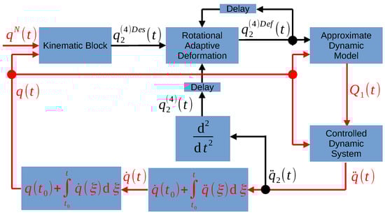
Figure 1. The structure of the order 4 adaptive backstepping controller: the delay corresponds to one cycle time of the digital controller.

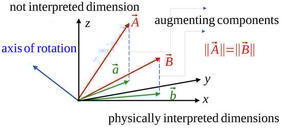
Figure 2. A 3D visualization of the method of interpolation with the angle of abstract rotations on the basis of [14].

Since the mathematical details were already explained in [14], here, we only briefly highlight that, for a great variety of physical systems, the method can be convergent. For simplicity, instead of rotations, a simple manipulation with a real parameter $\alpha$ is calculated that evidently has similar effects.

Consider a differentiable function $\Psi \left(x\right):{\mathbb{R}}^n\mapsto {\mathbb{R}}^n$ for which we wish to obtain $x_{★}$, the solution of the problem $\Psi \left(x_{★}\right)=x^{Des}$ for a given $x^{Des}$. With a real parameter $\alpha \in \mathbb{R}$, generate an iteration from a starting point as $x_{i+1}=x_i+\alpha \left(x^{Des}-\Psi \left(x_i\right)\right)$. Qualitatively, it can be stated that the role of the correction $\alpha \left(x^{Des}-\Psi \left(x_i\right)\right)$ is “pushing” the sequence toward the desired value.

The difference between the solution and the elements of the generated sequence can be simply estimated if the sequence is already in the vicinity of the solution by first-order Taylor series estimation as $\Psi \left(x_i\right)\equiv \Psi (x_{★}+x_i-x_{★})\approx \Psi \left(x_{★}\right)+{\left.{\displaystyle \frac{\partial \Psi }{\partial x}}\right|}_{x_{★}}(x_i-x_{★})=x^{Des}+{\left.{\displaystyle \frac{\partial \Psi }{\partial x}}\right|}_{x_{★}}(x_i-x_{★})$, as follows:

$$x_{i+1}-x_{★}\approx \left(I+\alpha {\left.{\displaystyle \frac{\partial \Psi }{\partial x}}\right|}_{x_{★}}\right)(x_i-x_{★}).$$

(7)

For simplicity, let us introduce the notation $M:={\left.{\displaystyle \frac{\partial \Psi }{\partial x}}\right|}_{x_{★}}$. If the matrix in (7) is contractive, the sequence will approach the solution. For proving contractivity, various matrix norms can be considered that are induced by vector norms. A typical possibility is the square root of the maximal eigenvalue of the symmetric positive semidefinite matrix ${(I+\alpha M)}^T(I+\alpha M)$ as

$$x^T{(I+\alpha M)}^T(I+\alpha M)x=x^T\left[I+\alpha \left(M^T+M\right)+{\alpha }^2{M}^{T}M\right]x\ge 0.$$

(8)

Evidently, if each eigenvalue of the symmetric matrix $(M^T+M)$ is different from zero and has the same sign, with a small positive or negative parameter $\alpha$, the contractivity for an arbitrary real vector x can be achieved. The practical significance of this condition can be easily understood if we consider the geometric interpretation of the scalar product of vectors $\Delta x$, and $\Delta \Psi :=\Psi (x+\Delta x)-\Psi \left(x\right)\approx {\displaystyle \frac{\partial \Psi }{\partial x}}\Delta x$, as follows:

$$\Delta x^T\Delta \Psi =\parallel \Delta x\parallel ·\parallel \Delta \Psi \parallel cos\phi \approx \Delta x^T{\displaystyle \frac{\partial \Psi }{\partial x}}\Delta x,$$

(9)

in which $\phi$ denotes the angle between these vectors. It can be said that $\Psi \left(x\right)$ is locally approximately direction keeping if this scalar product is positive. If the scalar product is negative, we can say that the direction of $\Delta \Psi$ is approximately opposite to that of $\Delta x$. These concepts can be regarded as the multidimensional generalizations of the single-variable monotonic increasing or monotonic decreasing functions. Since each matrix can be decomposed to a symmetric and a skew symmetric part as $A={\displaystyle \frac{1}{2}}\left(A+A^T\right)+{\displaystyle \frac{1}{2}}\left(A-A^T\right)$ and in (9), due to the symmetry in the indices of $\Delta x$, the skew symmetric part does not give a contribution, the appearance of the symmetric part of the partial derivative in (8) can be related to this concept.

Of course, it cannot be stated that this sequence will converge to an arbitrary physical system. However, in many practical cases, the possibility of convergence is given. For instance, in the dynamic model of robots, the inertial matrix is symmetric positive definite. Therefore, for fully actuated robots, the method can work. In certain underactuated mechanical systems as, e.g., that described in Figure 3, in certain regions, the appropriate effects of the control force can be different from each other, but the appropriate sign can be known in advance. Additionally, in driving a car, the roles of the accelerator and brake pedals will not be confused if the motion is free of slips. A small modification of the angle of the steering wheel always has consistent effects. In chemical systems, increasing or decreasing the ingress rate of certain reagents can be influenced consistently by dealing with the valves. Here, in the considered simple example of an underactuated system, the method can be used too.

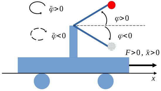
Figure 3. A typical underactuated mechanical system the control of which can be tackled by the suggested method.

Another mathematical interpretation can be obtained if we assume that M has the special Jordan canonical form (e.g., [19]) in which only order 1 eigenvectors occur; i.e., the space ${\mathbb{C}}^n$ can be spanned by the usual (not generalized) eigenvectors of M (this requirement is important since, generally, for an eigenvalue $\lambda$ of the matrix M, it can be stated only that $\left|\lambda \right|\le \parallel M\parallel$). In this case, an arbitrary vector can be expressed as the linear combination of such eigenvectors that can be normalized to have a unit norm. Then

$$\begin{array}{cc}\hfill & {\mathbb{C}}^n\ni x=\sum _{\ell }{x}_{\ell }{e}^{(\ell )},\parallel e^{(\ell )}\parallel =1\hfill \\ \hfill & Mx=\sum _{\ell }{x}_{\ell }{\lambda }_{\ell }{e}^{(\ell )},\hfill \\ \hfill & \parallel Mx\parallel =∥\sum _{\ell }{x}_{\ell }{\lambda }_{\ell }{e}^{(\ell )}∥\le max\left\{\right|{\lambda }_{\ell }\left|\right\}\sum _{\ell }|x_{\ell }|=max\{|{\lambda }_{\ell }{\left|\right\}\parallel x\parallel }_1.\hfill \end{array}$$

(10)

Then

$$(I+\alpha M)x=\sum _{\ell }{x}_{\ell }(1+\alpha {\lambda }_{\ell })e^{(\ell )}$$

(11)

corresponds to shifting the eigenvalues by 1. According to Figure 4, if the real part of each eigenvector is simultaneously either positive or negative, contraction can be achieved.

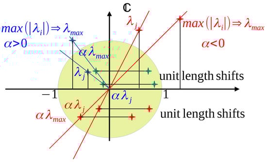
Figure 4. The convergence possibilities for the case $\forall \Re \left({\lambda }_{\ell }\right)>0$, $\alpha <0$, or the case $\forall \Re \left({\lambda }_{\ell }\right)<0$, $\alpha >0$, if the order 1 eigenvectors of M can span the whole linear space.

Formally, the method is related to Stefan Banach’s fixed point theorem if we consider the function $\Phi \left(x\right):=\alpha \Psi \left(x\right)-\alpha x^{Des}+x$ of which $x_{★}$ is a fixed point since $\Phi \left(x_{★}\right)=\alpha \Psi \left(x_{★}\right)-\alpha x^{Des}+x_{★}=x_{★}$.

The sequence generated by this function as $\{x_1;x_2=\Phi \left(x_1\right);\dots ;x_{i+1}=\Phi \left(x_i\right);\dots \}$ converges to $x_{★}$ if $\Phi \left(x\right)$ realizes a contractive mapping; i.e., $\exists 0\le K<1$ real number so that $\forall x,y$$\parallel \Phi \left(x\right)-\Phi \left(y\right)\parallel \le K\parallel x-y\parallel$. For the investigations tackling contractivity, the partial derivative ${\displaystyle \frac{\partial \Phi }{\partial x}}=\alpha {\displaystyle \frac{\partial \Psi }{\partial x}}+I$ must be considered.

In the box “Controlled Dynamic System”, the exact system model is used for simulation purposes. The method outlined in Figure 1 corresponds to the scheme of a special iterative learning in which, during one digital control step, a single step of the adaptive iteration can be executed. Its convergence under wide conditions can be guaranteed by using Stefan Banach’s fixed point theorem.

In the sequel, the dynamic model of the controlled system is considered.

3. The Dynamic Model of the Controlled System

The controlled system is outlined in Figure 5. In this model, no dissipative terms are taken into account from which it is expected that it is less stable than the damped ones. According to the equations of motion given in Figure 5, in which the masses of the springs are neglected, we have an order 2 system since, in any time instant, the ${\ddot{q}}_1\left(t\right),{\ddot{q}}_2\left(t\right)$ second time derivatives are determined by the model. However, if we wish to control the motion of the mass point $m_2$ by the control force $Q_1$, it can be observed that $Q_1$ does not have an immediate effect on ${\ddot{q}}_2\left(t\right)$. Evidently, ${\ddot{q}}_2\left(t\right)$ must be differentiated at least twice by the time to make ${\ddot{q}}_1\left(t\right)$ appear in the equation. Since ${\ddot{q}}_1\left(t\right)$ is immediately determined by $Q_1\left(t\right)$, the relative order of the control task is 4. The details were taken into account in the design of the backstepping controller that resulted in (6).

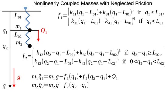
Figure 5. The structure and the dynamic model of the controlled system ($f_1$ and $f_2$ denote the springs’ pushing/pulling forces).

It should be noted that this relatively simple example serves as a good paradigm of realistic tasks. Normally, the components of machines are not ideally rigid; therefore, they have some additional degree of freedom that is not driven directly, and the connected components are apt to vibrate. The strongly asymmetric behavior of the springs against compression and dilatation at their zero force lengths is quite typical in the practice.

In Figure 6, the experimental setup is outlined in which the spring considered here was used. For this spring, only the parameters $k_{11}$ and $k_{12}$ were measured. These identical springs have a “dense” screwing structure; that is, it is easy to pull them, but against compression, the bulk material’s elastic parameters become relevant. Normally, they can be used with some bias to evade the appearance of the bulk effects. In the setup in Figure 6, such a compression can be evaded, but in the situation described in Figure 5, it may occur. In the model, this asymmetric hardening is represented by an order 6 polynomial and the huge coefficient $k_{41}$, $k_{42}$ (these are fictitious values). Additionally, a linear model with the coefficients ${\widehat{k}}_{41}$ and ${\widehat{k}}_{42}$ was considered. According to these asymmetries, certain model parameter errors may be quite insignificant or very significant, depending on the actual situation in the control. Other parameters’ estimation errors may have less significant effects in the control applications.

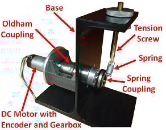
Figure 6. The “realistic spring model”: the spring considered here was in use in an experimental setup designed for studying different control situations (courtesy by Bence Varga of Óbuda University).

Making the derivations, our model yields the results as

$$\begin{array}{cc}\hfill & m_2{\stackrel{⃛}{q}}_2=-f_2^{\prime }(q_2-q_1)({\dot{q}}_2-{\dot{q}}_1)\hfill \end{array}$$

(12a)

$$\begin{array}{c}\hfill m_2{q}_2^{\left(4\right)}=-f_2^{″}(q_2-q_1){({\dot{q}}_2-{\dot{q}}_1)}^2-f_2^{\prime }(q_2-q_1)({\ddot{q}}_2-{\ddot{q}}_1).\end{array}$$

(12b)

From the equation given in Figure 5, ${\ddot{q}}_1$ can be substituted into (12b) and the control force $Q_1$ that is necessary to achieve the desired $q_2^{\left(4\right)Des}$ can be expressed as

$$\begin{array}{cc}\hfill & Q_1={\displaystyle \frac{m_1{m}_2}{f_2^{\prime }(q_2-q_1)}}{q}_2^{\left(4\right)Des}+\hfill \\ & {\displaystyle \frac{1}{f_2^{\prime }(q_2-q_1)}}\left\{m_1{f}_2^{″}(q_2-q_1){({\dot{q}}_2-{\dot{q}}_1)}^2+m_1{f}_2^{\prime }{\ddot{q}}_2\right.\hfill \\ \hfill & \left.-f_2^{\prime }(q_2-q_1)\left[m_{1}g-f_1\left(q_1\right)+f_2(q_2-q_1)\right]\right\}.\hfill \end{array}$$

(13)

To evade further complications to (13), ${\ddot{q}}_2$ can be substituted from the equation given in Figure 5. This can be done conveniently if, in the simulation program, the mathematical functions $f_1\left(x\right)$, $f_2\left(x\right)$, $f_2^{\prime }\left(x\right)$, and $f_2^{″}\left(x\right)$ are represented as program functions.

In the simulations in which the strict validity of the analytical form of (13) is assumed, this equation is used in two forms: with the exact parameters and in the form in which the parameters under significance investigations take their approximate values. In this case for determining the extent of the necessary full deformation of the “desired” $q_2^{\left(4\right)Des}$ for the achieved $q_2^{\left(4\right)}\left(t\right)$ value in the physical state of the controlled system defined by $q_1,q_2,{\dot{q}}_1,{\dot{q}}_2$, under the effect of force, $Q_1$ can be computed from the exact and the approximate models too. In this case, the rotational metric for comparing the values of $q_2^{\left(4\right)Des}$ and $q_2^{\left(4\right)Def}$ can also be computed.

Another possibility is the comparison of the force needs of the actual model and the approximate model for the achieved $q_2^{\left(4\right)}$, if we are able to calculate these forces. For this comparison, a similar rotational metric can be applied.

For showing the applicability of the significance evaluating method for more complex, more practical cases in which the precise analytical deduction of (13) is too laborious or hopeless due to other reasons—therefore, the force need of the exact model cannot be computed—the significance of the effects of modeling inconsistencies and imprecisions together can still be computed by the comparison of the pairs $q_2^{\left(4\right)Des}$ and $q_2^{\left(4\right)Def}$. For demonstrating this situation, the equations of motion in Figure 5 have been completed by two friction force terms $-b_1{\dot{q}}_1$ and $-b_2{\dot{q}}_2$ as follows:

$$\begin{array}{cc}\hfill & {\ddot{q}}_1=g+{\displaystyle \frac{-f_1\left(q_1\right)+f_2(q_2-q_1)-b_1{\dot{q}}_1+Q_1}{m_1}}\hfill \\ \hfill & {\ddot{q}}_2=g+{\displaystyle \frac{-f_2(q_2-q_1)-b_2{\dot{q}}_2}{m_2}}.\hfill \end{array}$$

(14)

However, the precise consequences of the additional friction terms are not computed in $q_2^{\left(4\right)}$ according to (14). Instead of that, as an incomplete approximation, (13) is used in the adaptive control. In this context, the force need of the exact model is not computed. However, the pair $q_2^{\left(4\right)Des}$ and $q_2^{\left(4\right)Def}$ can be used for computing the significance of the various parameter imprecisions.

On the above basis, in the Section 4, simulation investigations will be presented.

4. Simulation Investigations

The simulation investigations were made for the dynamic model parameters given in Table 1. In the control, the $K_1=K_2=K_3=K_4=K_5=\Lambda$ setting was used with a common exponent in Table 2.

Table 1. The dynamic parameters of the exact model.

Parameter	Notation	Unit	Exact Value
Linear stiffness of spring 1	$k_{11}$	N·m−1	1611
Cubic stiffness of spring 1	$k_{31}$	N·m−3	0
Order 6 stiffness of spring 1	$k_{41}$	N·m−6	${10}^6$
Mass of point 1	$m_1$	kg	2
Zero force length of spring 1	$L_{01}$	m	$0.02$
Linear stiffness of spring 2	$k_{12}$	N·m−1	1611
Cubic stiffness of spring 2	$k_{32}$	N·m−3	0
Order 6 stiffness of spring 2	$k_{42}$	N·m−6	${10}^6$
Mass of point 2	$m_2$	kg	$1.8$
Zero force length of spring 2	$L_{02}$	m	$0.02$
Gravitational acceleration	g	m·s−2	$9.81$
Additional friction coefficient for point 1	$b_1$	N·s·m−1	various
Additional friction coefficient for point 2	$b_2$	N·s·m−1	various

Table 2. The control parameters.

Parameter	Notation	Unit	Value
Common decay exponent	$\Lambda$	s−1	40
Common norm in the adaptive deformation	$R_a$	m·s−4	${10}^6$
Rotational angle interpolation factor	${\lambda }_a$	Nondimensional	$0.16$
Common norm in the significance calculation	$\mathfrak{R}$	m·s−4 or N	${10}^{22}$
Cycle time/time resolution	$\delta t$	s	${10}^{-4}$

The nominal trajectory was generated by shifting that of a van der Pol oscillator [20] starting from the vicinity of its unstable equilibrium point and approaching nonlinear oscillations in a limit cycle.

At first, the $b_1=b_2=0$ case was investigated for which both the force-based and the 4th derivative-based significance investigations can be simultaneously performed and compared with each other. Following that, the more complex cases with $b_1\ne 0$ and $b_2\ne 0$ are considered with the derivative-based significance investigations.

4.1. Investigations for the Strictly Valid Analytical Model Form

At first, the non-adaptive controller’s operation was investigated using an exact dynamic model. Since the various controllers apply various error feedback terms, the “control situation” in general can be defined by the nominal trajectory to be tracked. The results reveal the precision of the operation of the basic backstepping controller with the control parameter settings applied. The method can be checked by considering the effects of the adaptation mechanism when no adaptation is needed. The nominal trajectory was generated by a van der Pol oscillator model of equation of motion in (15) with ${\tilde{m}}_1=1$ kg, $k_1=$500 N·m⁻¹, $a_1=0.03$ m, and $b_{11}=150$ N·s·m⁻³.

$$\ddot{q}={\displaystyle \frac{-k_{1}q+b_{11}\left(a_1^2-q^2\right)\dot{q}}{{\tilde{m}}_1}},q\left(0\right)=0,\dot{q}\left(0\right)=0.3\mathrm{m}·{\mathrm{s}}^{-1}$$

(15)

4.1.1. Checking the Effects of the Adaptation Mechanism in the Case of the Exact Dynamic Model

In the case of an exact dynamic model, in principle, no adaptive approach is needed. However, switching on adaptation can cause some refinement in the controller’s operation, and the obtained significance metrics determine some “minimum” so that only the higher values can capture physically interesting effects. In this step, the non-adaptive and the adaptive controllers are compared with each other. The important results are revealed in Figure 7, Figure 8 and Figure 9.

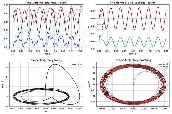
Figure 7. The trajectories of the free (in the top LHS) and the non-adaptive controlled motion (in the top RHS); the phase trajectories for the non-adaptive controller using the exact dynamic model (in the bottom).

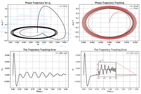
Figure 8. The phase trajectories for the adaptive motion using the exact dynamic model (in the top); trajectory tracking error for the exact dynamic model for the non-adaptive (in the bottom LHS) and the adaptively controlled motion (in the bottom RHS).

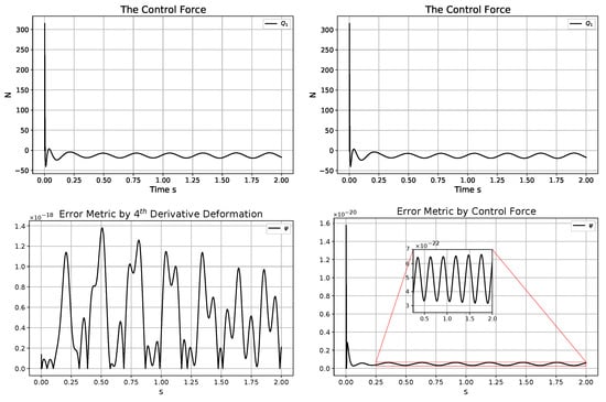
Figure 9. The control forces in the non-adaptive (in the top LHS) and the adaptive (in the top RHS) controllers; significance metrics for the adaptive controller related to $q_2^{\left(4\right)}$ (in the bottom LHS) and the force-based metric when the exact dynamic model was in use (in the bottom RHS).

It can be seen that the free and the controlled cases were comparable in the main frequency component of motion, but the controller caused quite drastic modification of the trajectories. The subtle differences between the operations of the non-adaptive and adaptive controllers are well visualized in the phase trajectories.

Since the maximal velocity of motion was about $0.3$ m·s⁻¹, the digital time resolution of $\delta t={10}^{-4}$ s was a reasonable choice to reveal subtle details of motion: during a digital control cycle time, this could result in $3\times {10}^{-5}$ m displacement. The adaptation mechanism reduced the tracking error from $1$ mm to ${10}^{-5}$ m. The diagrams of the control forces do not provide easily observable differences. It can be stated that the error metrics in the range $[0,1.4\times {10}^{-18}]$ rad for the fourth-order derivatives and $[0,6.6\times {10}^{-22}]$ rad for the control forces can be related to the precision of the adaptive controller and do not convey information on the effects of parameter modeling errors that are revealed by greater numbers. It can be stated that the “not necessary adaptivity” in the case of the exact model did not cause any problem. It only slightly improved the tracking properties of the controller. The control parameter settings applied provide an appropriate basis for further investigations. In this subsection, the effects of individual parameters’ errors are investigated when the exact model form is assumed to be valid. In the sequel, only the operation of the adaptive controller is considered. The parameters of the “assumed model” are kept constant, and the “exact ones” not known by the controller are modified.

4.1.2. Checking the Significance of the Error of Model Parameter $m_1$

In this calculation, the actual $m_1=3$ kg was in use instead of the assumed value $2$ kg. Figure 10 does not reveal drastic differences in the free motion and the controlled adaptive solution. The same can be said on the basis of Figure 11: neither the tracking error nor the significance metrics show considerable variations though the relative difference between the model and the exact value of parameter $m_1$ is quite considerable. The consecutive adaptive deformations in the control cycles were very close to the identity operator. On this basis, it can be stated that, in the case of the present circumstances, no high precision is needed for modeling parameter $m_1$.

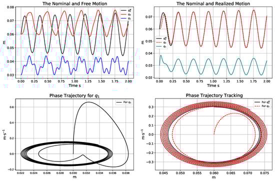
Figure 10. The trajectories of the free (in the top LHS) and the adaptive controlled (in the top RHS) motion; the phase trajectories for the adaptive controller using the actual model parameter $m_1=3$ kg instead of the assumed value $2$ kg (in the bottom).

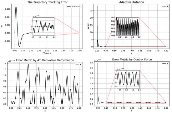
Figure 11. Trajectory tracking error (in the top LHS); angle of the adaptive abstract rotations (in the top RHS); significance metrics for the adaptive controller related to $q_2^{\left(4\right)}$ (in the bottom LHS) and the force-based metric for the adaptive controller using the actual model parameter $m_1=3$ kg instead of the assumed value $2$ kg (in the bottom RHS).

4.1.3. Checking the Significance of the Error of the Model Parameter $m_2$

In these simulations, the actual value of the parameter $m_2$ was $3$ kg instead of the assumed $1.8$ kg. Figure 12 and Figure 13 reveal that the free motion belonging to the same initial conditions drastically changed, while the trajectory tracking error of the adaptively controlled motion remained very small, and tracking the phase trajectory for the variable $q_2$ remained precise too. The comparison with Figure 9 reveals that a significance metric in the peaks after $1$ s and $1.25$ s increased from about $1.1\times {10}^{-18}$ to $1.3\times {10}^{-18}$ rad. This variation remained within the same order of magnitude, but it is definitely observable.

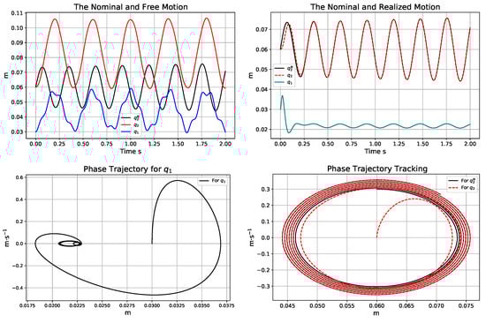
Figure 12. The trajectories of the free (in the top LHS) and the adaptively controlled (in the top RHS) motion; the phase trajectories for the adaptive controller (in the bottom) using the actual model parameter $m_2=3$ kg instead of the assumed value $1.8$ kg.

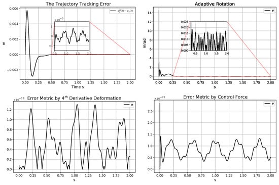
Figure 13. Trajectory tracking error (in the top LHS); angle of the adaptive abstract rotations (in the top RHS); significance metrics for the adaptive controller related to $q_2^{\left(4\right)}$ (in the bottom LHS) and the force-based metric (in the bottom RHS) for the adaptive controller using the actual model parameter $m_2=3$ kg instead of the assumed value $1.8$ kg.

The peak value of the force-based significance metric increased from $6.5\times {10}^{-22}$ rad to $1.25\times {10}^{-21}$ rad, and the shape of the curve shows a quite different structure from its counterpart in Figure 9. It can be stated that, in the given control task and circumstances, the precise estimation of the parameter $m_2$ has greater significance than that of $m_1$.

4.1.4. Checking the Significance of the Error of Parameters $k_{11}$ and $k_{12}$

In this simulation, the actual value of these parameters was $1000$ N·m⁻¹ instead of the assumed value $1611$ N·m⁻¹.

Figure 14 and Figure 15 reveal considerable differences in the free motion in the error metrics, while the adaptive controller yielded precise trajectory and phase trajectory tracking.

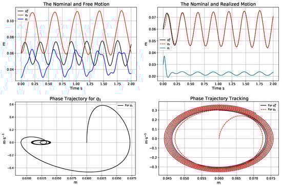
Figure 14. The trajectories of the free (in the top LHS) and the adaptively controlled (in the top RHS) motion; the phase trajectories for the adaptive controller using the actual model parameter $k_{11}=k_{12}=1000$ N·m⁻¹ instead of the assumed value $1611$ N·m⁻¹ (in the bottom).

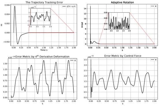
Figure 15. Trajectory tracking error (in the top LHS); angle of the adaptive abstract rotations (in the top RHS); significance metrics for the adaptive controller related to $q_2^{\left(4\right)}$ (in the bottom LHS) and the force-based metric for the adaptive controller using the actual model parameter $k_{11}=k_{12}=1000$ N·m⁻¹ instead of the assumed value $1611$ N·m⁻¹ (in the bottom).

Figure 16 reveals that, in this case, the “desired value” was drastically deformed by the adaptive controller.

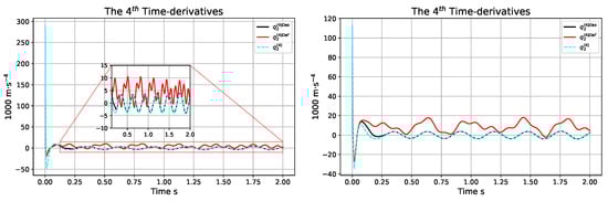
Figure 16. The order 4 time derivatives of the adaptive controller in the case of using the exact model parameters (LHS) and the actual model parameters $k_{11}=k_{12}=1000$ N·m⁻¹ instead of the assumed value $1611$ N·m⁻¹ (RHS).

It is important to note that, in the above calculations, with an exception of the data described in Figure 14 for a short time in the beginning, spring 1 was used in a “biased manner”; i.e., the effects of the asymmetric hardening of the spring did not occur. In the short period of the unbiased operation of spring 1, the motion remained within the physically interpreted $q_1>0$ range. According to the simulations for capturing the rough asymmetry in the spring force vs. dilatation or compression, the order 6 polynomial model in Figure 5 was too smooth about 0 compression. To produce a more drastically asymmetric model, only in the forthcoming parts of the paper, the model given in Figure 5 was modified.

4.1.5. Checking the Significance of the Error of the Stiffness Parameter for Compression

In these simulations, the previously used compression model was modified as follows:

$$\begin{array}{cc}\hfill & f_1={\widehat{k}}_{41}(q_1-L_{01})if{q}_1<L_{01}\hfill \\ \hfill & f_2={\widehat{k}}_{42}(q_2-q_1-L_{02})if{q}_2-q_1<L_{02}.\hfill \end{array}$$

(16)

For guaranteeing strong asymmetry with the parameters $k_{11}=k_{12}=1611$ N·m⁻¹, the settings ${\widehat{k}}_{41}={\widehat{k}}_{42}={10}^6$ N·m⁻¹ were applied in the exact model. The nominal trajectory was shifted too to obtain lucid effects.

Figure 17 testifies that the adaptation mechanism with the exact model resulted in tracking precision and significance metrics similar to that of the previous model: significance metric according to the 4th time derivatives about $1.4\times {10}^{-18}$ rad; the force based metric yielded $6.5\times {10}^{-22}$ rad values; and the tracking precision was about ${10}^{-5}$ m.

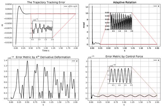
Figure 17. Trajectory tracking error (in the top LHS); angle of the adaptive abstract rotations (in the top RHS); significance metrics for the adaptive controller related to $q_2^{\left(4\right)}$ and the force-based metric for the adaptive controller using the exact model (in the bottom).

The actual values of the parameters ${\widehat{k}}_{41}={\widehat{k}}_{41}$ in the forthcoming calculations were $1.02\times {10}^6$ N·m⁻¹ instead of the assumed ${10}^6$ N·m⁻¹. The controller was just able to produce acceptable tracking. It seems to be expedient to show each available computation detail. Figure 18 testifies that the realized motion happened with compressed spring 1 and remained in the physically interpreted $q_1>0$ range. According to Figure 19, the tracking error became approximately 10 times higher than its counterparts in the previous simulations, but it remained acceptable. The fourth derivative-based error metric increased by an order of magnitude; the force-based one increased from $6.5\times {10}^{-22}$ rad to $1.3\times {10}^{-20}$ rad. Figure 20 indicates that the adaptation mechanism was not perfect, though it caused considerable adaptive deformations.

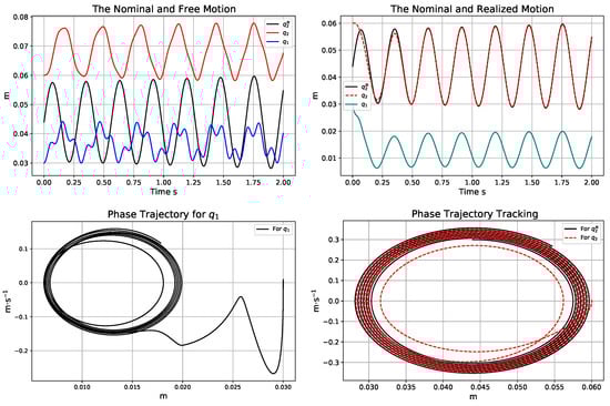
Figure 18. The trajectories of the free (in the top LHS) and the adaptively controlled (in the top RHS) motion; the phase trajectories for the adaptive controller using the actual model parameter ${\widehat{k}}_{14}={\widehat{k}}_{24}=1.02\times {10}^6$ N·m⁻¹ instead of the assumed value ${10}^6$ N·m⁻¹ (in the bottom).

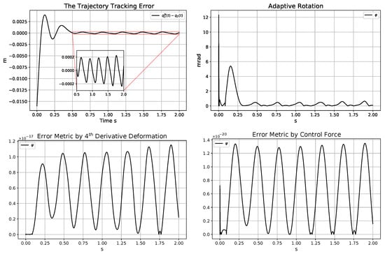
Figure 19. Trajectory tracking error (in the top LHS); angle of the adaptive abstract rotations (in the top RHS); significance metrics for the adaptive controller related to $q_2^{\left(4\right)}$ (in the bottom LHS) and the force-based metric for the adaptive controller using the actual model parameter ${\widehat{k}}_{14}={\widehat{k}}_{24}=1.02\times {10}^6$ N·m⁻¹ instead of the assumed value ${10}^6$ N·m⁻¹ (in the bottom).

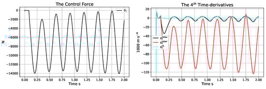
Figure 20. The control forces and the order four time derivatives of the adaptive controller in the case of using the actual model parameters ${\widehat{k}}_{14}={\widehat{k}}_{24}=1.02\times {10}^6$ N·m⁻¹ instead of the assumed value ${10}^6$ N·m⁻¹ (RHS).

5. Investigations for the Corrupted Model Form

In these simulations, the model form belonging to (16) was applied with the viscous friction parameters $b_1=b_2=20$ N·s·m⁻¹. Though these parameters could result in a relative order 3 control, due to the approximate model applied, we developed an approximate relative order 4 controller. The nominal trajectory was so shifted that both compression and dilatation were necessary for spring 1. In this case, the calculation of the force-based metric was irrelevant.

Figure 21 indicates smooth and precise adaptive motion; the adaptive mechanism was able to correct the effects of modeling errors. In Figure 22, it can be well observed, e.g., at the time instants $t=0.25$ s and $t=1.25$ s, that the variable $q_1$ crossed the border of the “stiff” and “soft” spring operation modes: before $t=0.25$ s, huge negative compression forces were applied for spring 1 since, for $q_1<L_{01}$, this spring was drastically compressed. Before $t=1.25$ s in the $q_1>L_{01}$ region, the spring was softly pulled for which no considerable control force was necessary. In comparison with Figure 17, it can be stated that using the inexact model form did not have significant effects on the operation of the controller.

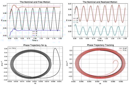
Figure 21. The trajectories of the free (in the top LHS) and the adaptively controlled (in the top RHS) motion; the phase trajectories for the adaptive controller using the corrupted model (in the bottom).

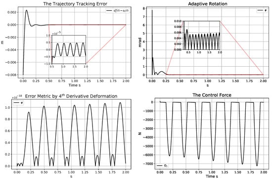
Figure 22. Trajectory tracking error (in the top LHS); angle of the adaptive abstract rotations (in the top RHS); significance metric for the adaptive controller related to $q_2^{\left(4\right)}$ (in the bottom LHS) and the control force (in the bottom RHS) for the adaptive controller using the corrupted model form.

6. Conclusions

In this paper, the potential application of a variant of the Fixed Point Iteration-Based Adaptive Controllers was investigated in model-based control. The main point was the introduction of a “parameter estimation significance metric” through the use of which the very laborious and sometimes unsolvable task, the estimation of the individual model parameters, can be avoided. Depending on the complexity of the available dynamic model of the physical system under control, either in the significance of the precision of the estimation of a given individual parameter or in the case of an imprecise model form, the consequences of the approximate model as a whole can be estimated. The adaptive controller can force the system to track the prescribed nominal trajectory, therefore bringing about the “actual control situations” in which the consequences of the estimation errors are of interest. One component of the adaptive control is a “rotational block” that can create a multidimensional orthogonal (rotation) matrix that rotates arrays of identical Frobenius norm into each other. Since, in a recent publication under review, it was proved that the angle of the necessary rotation satisfies the criteria of a metric in a metric space, even in quite complicated nonlinear and multidimensional cases, this simple value can serve as a metric.

To exemplify the method, an underactuated nonlinear system of 2 degree of freedom and relative order 4 was controlled by a special adaptive backstepping controller that was designed on a purely kinematic basis. The nominal trajectory to be tracked was dynamically “rich”: it was the trajectory of a van der Pol oscillator that commenced its motion in the vicinity of its unstable equilibrium point and approached nonlinear oscillations in a limit cycle. The controlled system contained a coupled spring of strongly non-symmetric stiffness against compression or dilatation without stabilizing viscous terms. This simple model was rich enough to exemplify parameters that require precise identification because their error produces quite significant consequences and other parameters that do not require very precise identification. It was found that the method provided the dynamic models with sensitive and reliable parameter sensitivity estimation metrics.

The generally valid conclusions can be summarized as follows:

• In general, the control task can be defined by the nominal trajectory to be tracked, and the initial conditions of the state of the controlled system.
• The occurring control situations that evolve in time depend on the control task, on the qualitative properties and the parameters of the fundamental control approach (in our case a backstepping controller), and on the qualitative properties and parameters of the complementary adaptation mechanisms by which the basic controllers were “escorted”. In our case, it was a fixed point iteration-based adaptive controller that can be applicable for numerous physical systems, and can cooperate with any kinematically designed basic control method that uses either backstepping solution, PID feedback, control Lyapunov function-based approach, or some robust variable structure/sliding mode solution.
• The significance of the estimation precision of a given parameter of an analytically formulated model can be defined only within a given control situation. The control situation depends on numerous number of parameters. However, if the trajectory tracking of the given adaptive solution is precise enough, this concept can be related to the control task.
• The here suggested and investigated estimation precision significance metric is not an “absolute numerical value”. It contains a free parameter $\mathfrak{R}$ that normally must be a large value that guarantees that the appropriate arrays in comparison can be augmented with one dimension.
• It is expedient to run the calculations for the adaptive controller using the exact dynamic model to determine the minimal significance values that cannot be associated with physically interpreted parameter estimation errors. The calculated significance of the parameter estimation errors can be compared with these minimum values.
• Following the above preparation, the significance of the errors caused by analytically inappropriate model forms can be estimated by the suggested method.

References

- Szalay, P.; Eigner, G.; Kovács, L.A. Linear matrix inequality-based robust controller design for type-1 diabetes model. Ifac Proc. Vol. 2014, 47, 9247–9252. [Google Scholar] [CrossRef]
- Man, C.D.; Micheletto, F.; Lv, D.; Breton, M.; Kovatcher, B.; Cobelli, C. The UVA/PADOVA type 1 diabetes simulator: New features. J. Diabetes Sci. Technol. 2014, 8, 26–34. [Google Scholar] [CrossRef] [PubMed]
- Ledzewicz, U.; Schättler, H. A synthesis of optimal controls for a model of tumor growth under angiogenic inhibitors. In Proceedings of the 44th IEEE Conference on Decision and Control, and the European Control Conference 2005, Seville, Spain, 12–15 December 2005; pp. 934–939. [Google Scholar]
- Sápi, J.; Drexler, D.A.; Kovács, L. Comparison of mathematical tumor growth models. In Proceedings of the 2015 IEEE 13th International Symposium on Intelligent Systems and Informatics (SISY 2015), Subotica, Serbia, 17–19 September 2015; pp. 323–328. [Google Scholar]
- Ionescu, C.M.; Mendonca, T.F.; Kovacs, L. Critically safe general anaesthesia in closed loop: Availability and challenges. In Proceedings of the 9th IFAC Symposium on Biological and Medical Systems (IFAC BMS 2015), Berlin, Germany, 31 August–2 September 2015; pp. 551–556. [Google Scholar]
- Sápi, J.; Ferenci, T.; Drexler, D.A.; Kovács, L. Tumor model identification and statistical analysis. In Proceedings of the 2015 IEEE International Conference on Systems, Man, and Cybernetics, Hong Kong, China, 9–12 October 2015; pp. 2481–2486. [Google Scholar] [CrossRef]
- Tar, J.K.; Bitó, J.F.; Nádai, L.; Machado, J.A.T. Robust Fixed Point Transformations in adaptive control using local basin of attraction. Acta Polytech. Hung. 2009, 6, 21–37. [Google Scholar]
- Armstrong, B.; Khatib, O.; Burdick, J. The explicit dynamic model and internal parameters of the PUMA 560 arm. In Proceedings of the IEEE Conference on Robotics and Automation, San Francisco, CA, USA, 7–10 April 1986; pp. 510–518. [Google Scholar] [CrossRef]
- Sciavicco, L.; Siciliano, B. Modeling and Control of Robot Manipulators; McGraw Hill: New York, NY, USA, 1996; 358p, p. 701. ISBN 0-07-057217-8. [Google Scholar] [CrossRef]
- Lyapunov, A.M. A General Task About the Stability of Motion. Ph.D. Thesis, University of Kazan, Tatarstan, Russia, 1892. [Google Scholar]
- Lyapunov, A.M. Stability of Motion; Academic Press: New York, NY, USA; London, UK, 1966. [Google Scholar]
- Gahinet, P.; Apkarian, P.; Chilali, M. Affine parameter-dependent Lyapunov functions and real parametric uncertainty. IEEE Trans. Autom. Control 1996, 41, 436–442. [Google Scholar] [CrossRef]
- Banach, S. Sur les opérations dans les ensembles abstraits et leur application aux équations intégrales (About the Operations in the Abstract Sets and Their Application to Integral Equations). Fundam. Math. 1922, 3, 1922. [Google Scholar] [CrossRef]
- Csandi, B.; Galambos, P.; Tar, J.K.; Györök, G.; Serester, A. A novel, abstract rotation-based fixed point transformation in adaptive Control. In Proceedings of the 2018 IEEE International Conference on Systems, Man, and Cybernetics (SMC), Miyazaki, Japan, 7–10 October 2018; pp. 2577–2582. [Google Scholar] [CrossRef]
- Rodrigues, O. Des lois géometriques qui regissent les déplacements d’ un systéme solide dans l’ espace, et de la variation des coordonnées provenant de ces déplacement considérées indépendent des causes qui peuvent les produire (Geometric laws which govern the displacements of a solid system in space: And the variation of the coordinates coming from these displacements considered independently of the causes which can produce them). J. Math. Pures Appl. 1840, 5, 380–440. [Google Scholar]
- Sparavalo, M.K. A method of goal-oriented formation of the local topological structure of co-dimension one foliations for dynamic systems with control. J. Autom. Inf. Sci. 1992, 25, 65–71. [Google Scholar]
- Kokotovic, P.V. The joy of feedback: Nonlinear and adaptive. IEEE Control. Syst. Mag. 1992, 12, 7–17. [Google Scholar] [CrossRef]
- Lozano, R.; Brogliato, B. Adaptive control of robot manipulators with flexible joints. IEEE Trans. Autom. Control 1992, 37, 174–181. [Google Scholar] [CrossRef]
- Dieudonné, J. Oeuvres de Camille Jordan I–IV (Colleceted Works by Camille Jordan); Gauthier-Villars: Paris, France, 1961; Available online: https://books.google.hu/books?id=HJ2R2UVJI5kC (accessed on 20 November 2024).
- van der Pol, B. Forced oscillations in a circuit with non-linear resistance. (Reception with reactive triode). Lond. Edinb. Dublin Philos. Mag. J. Sci. 1927, 3, 65–80. [Google Scholar] [CrossRef]
Disclaimer/Publisher’s Note: The statements, opinions and data contained in all publications are solely those of the individual author(s) and contributor(s) and not of MDPI and/or the editor(s). MDPI and/or the editor(s) disclaim responsibility for any injury to people or property resulting from any ideas, methods, instructions or products referred to in the content. |
© 2025 by the authors. Licensee MDPI, Basel, Switzerland. This article is an open access article distributed under the terms and conditions of the Creative Commons Attribution (CC BY) license (https://creativecommons.org/licenses/by/4.0/).