HawkFish Optimization Algorithm: A Gender-Bending Approach for Solving Complex Optimization Problems
Abstract
1. Introduction
- To create an algorithm inspired by the adaptive gender transition behavior of hawkfish, integrating dual fitness functions, dynamic clustering, and differentiated visual scopes.
- To improve the balance between exploration and exploitation in solving complex optimization problems with diverse landscapes.
- To incorporate dynamic clustering mechanisms to maintain population diversity and prevent premature convergence.
- To utilize the distinct behaviors and visual scopes of male and female fish to optimize the search process effectively.
- Several algorithms, such as MOPSO and Gazelle Optimization, exhibit convergence issues, particularly in high-dimensional or complex landscapes, leading to suboptimal solutions.
- Many approaches, including MOEA/D and SPEA2, rely on fixed or sensitive parameter settings that require extensive tuning and may not generalize well to diverse optimization scenarios.
- Algorithms like QDSA and Knacks of Evolutionary Mating face difficulties scaling to large objective spaces or adapting to highly dynamic optimization environments, limiting their effectiveness in real-world applications.
- Insufficient mechanisms for maintaining diversity in Pareto fronts, as noted in QDSA, MOPSO, and MOSA, reduce their ability to explore the solution space effectively and avoid stagnation.
- Dynamic Cluster Formation and Update
- b.
- Fitness Function Bending
- c.
- Dynamic Visual Scope
2. Proposed Method
2.1. Hawkfish Gender Bending
2.2. Mathematical Modeling
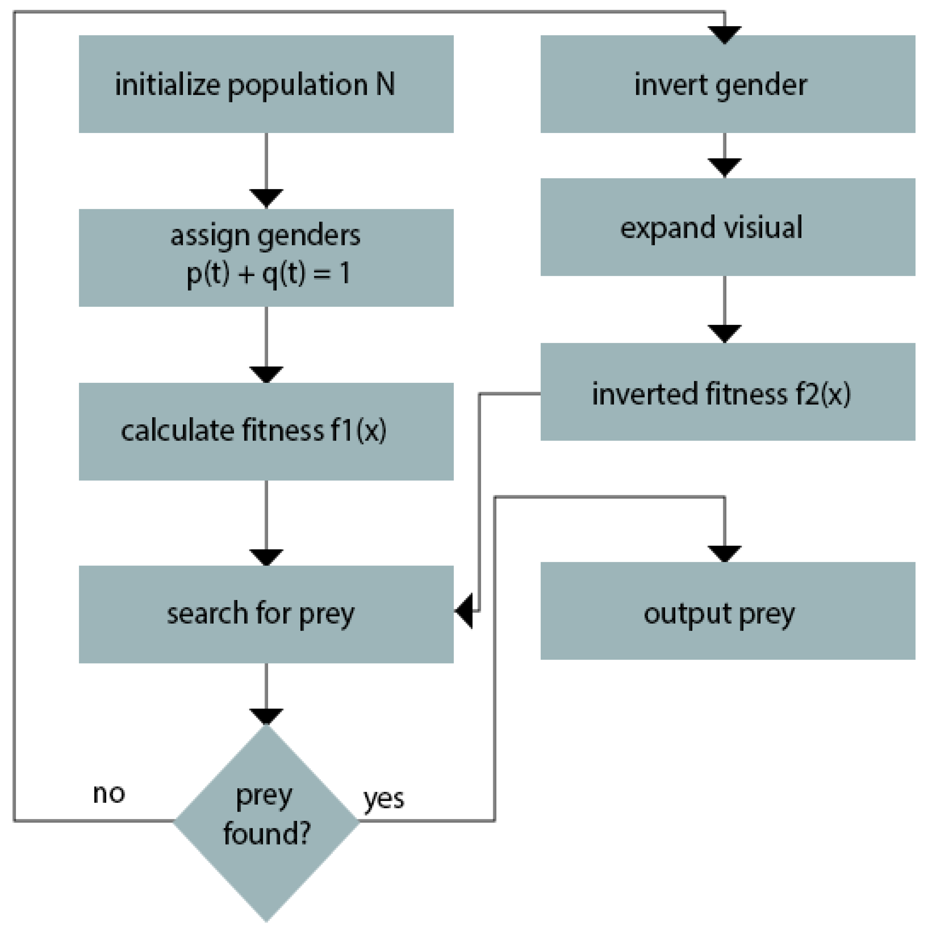
- Initialize the population:The algorithm begins by initializing a population of artificial fish, where each fish is represented by a vector of n dimensions. The population size is denoted as N.
- Evaluate the fitness:The fitness of each fish is evaluated using two fitness functions, f1(x) and f2(x), where x is the position vector of the fish.
- Fish movement:The movement of each fish is determined by the following equation:where x(i, j) is the jth element of the position vector of the ith fish, s(i, j) is the step size of the ith fish, and d(i, j) is the jth element of the direction vector of the ith fish. The step size and direction vector are determined based on the fitness of the fish.
- Update the fitness:After each movement, the fitness of each fish is re-evaluated using the two fitness functions.
- Dynamic fish clustering:Let the position vectors of the fish be represented as X = {x1, x2, …, xN}, where xi is the position of the ith fish.
- Distance matrix:Calculate the pairwise distance matrix D, where D(i, j) = ||xi − xj|| represents the distance between fish i and j.
- Clustering algorithm:Use a Euclidean-based distance-based clustering to partition X into k clusters C1, C2, …, Ck, such that:
- Cluster leaders:For each cluster Cp, identify the cluster leader:xp,best = arg max f(xi), where f(xi) is the fitness function value for fish i.
- Dynamic updates:Periodically recompute the clusters to adapt to the evolving distribution of fish in the search space.
- Fish learning:Each fish in a subpopulation learns from its neighbors using the following equation:where x(jbest, j) is the jth element of the position vector of the best fish in the subpopulation, and w is the learning coefficient.
- Update the step size and direction vector:The step size and direction vector of each fish are updated using the following equations:where α and β are learning coefficients, r is a random number between 0 and 1, xglobal(j) is the jth element of the position vector of the global best fish, and xlocal(j) is the jth element of the position vector of the local best fish.
- Repeat:Steps 2–6 are repeated until a stopping criterion is met, such as a maximum number of iterations or a threshold value for the fitness function.
| Algorithm 1: Search and Clustering |
| 1. Initialize parameters: N (population size), n (number of dimensions), k (number of subpopulations), α (Global learning coefficient), β (Local learning coefficient), w (Subpopulation learning coefficient), max_iterations 2. Initialize the population of artificial fish with random positions in the search space 3. For iter in range(max_iterations): 3.1. Evaluate the fitness of each fish using f1(x) and f2(x) 3.2. Update the position of each fish based on their fitness: For i in range(N) and j = 1, 2, …, n: x(i,j) = x(i,j) + s(i,j) × d(i,j) ∀j ∈ {1, 2, …, n}. 3.3. Re-evaluate the fitness of each fish after movement 3.4. Cluster the population into k subpopulations to increase diversity xp,best = arg max f(xi), where f(xi) is the fitness function value for fish i 3.5. Perform fish learning within subpopulations: For each subpopulation: For i in range(number of fish in subpopulation): x(i,j) = x(i,j) + w × (x(jbest,j) − x(i,j)) ∀j ∈ {1, 2, …, n}. 3.6. Update the step size and direction vector of each fish: For i in range(N): s(i,j) = s(i,j) + α·random(0,1) × r × (xglobal(j) − x(i,j)) ∀j∈{1, 2, …, n} d(i,j) = d(i,j) + β random(0,1) × r × (x(i,j) − xlocal(j) ∀j∈{1, 2, …, n} 4. Return the global best solution found |
- Divide the population P of artificial fish into 2 subpopulations: Pmale for male artificial fish and Pfemale for female artificial fish, where |Pmale| and |Pfemale| denote the sizes of the male and female subpopulations, respectively.
- Assign a unique visual scope Vmale to the male subpopulation Pmale and Vfemale to the female subpopulation Pfemale.
- Evaluate the availability of food in the search space, represented by a food metric F, which could be the average fitness of the population or another suitable measure.
- For each iteration t:
- Update the gender of each artificial fish f based on the availability of food F:If F > F_threshold, where F_threshold is a predefined threshold, change the gender of fish f. For example, if fish f is male, change it to female, and vice versa.
- For each artificial fish f in subpopulation Pmale or Pfemale, only consider other fish within the corresponding visual scope Vmale or Vfemale when evaluating the fitness and updating the position.
- The position update equation of artificial fish f in subpopulation Pmale or Pfemale can be represented as:Here, x_f(t) denotes the position of artificial fish f at iteration t, step_size is the step size, and x_center is the center of the corresponding subpopulation (Pmale or Pfemale).
- The center of the subpopulation Pmale or Pfemale can be calculated as:Here, x_j represents the position of the j-th artificial fish in the corresponding subpopulation (Pmale or Pfemale).
- When updating the position of artificial fish f in subpopulation P_dist (Pmale or Pfemale), only consider other fish within the visual scope Vmale or Vfemale:
- Find the set of neighboring fish N_f within the visual scope Vmale or Vfemale:
- Update the position of artificial fish f based on the information from neighboring fish N_f:
| Algorithm 2: Gender Switching Sub-Strategy |
| Initialize population P with positions and genders Set Vmale and Vfemale (unique visual scopes for male and female subpopulations) Set F_threshold (predefined threshold for food availability) Set max_iterations for t = 1 to max_iterations: Calculate food metric F (e.g., average fitness of the population) for each artificial fish f in P: if F > F_threshold: Change the gender of fish f (swap between male and female) if fish f is male: Find neighboring fish N_f within visual scope Vmale else: Find neighboring fish N_f within visual scope Vfemale Determine x_nbest (position of the best neighboring fish in N_f) Update position of fish f: x_f(t+1) = x_f(t) + step_size × (x_nbest − x_f(t)) Update fitness values for all fish in the population Check stopping criteria (e.g., convergence or maximum iterations reached) |
3. Results and Discussion
3.1. Implementation Environment
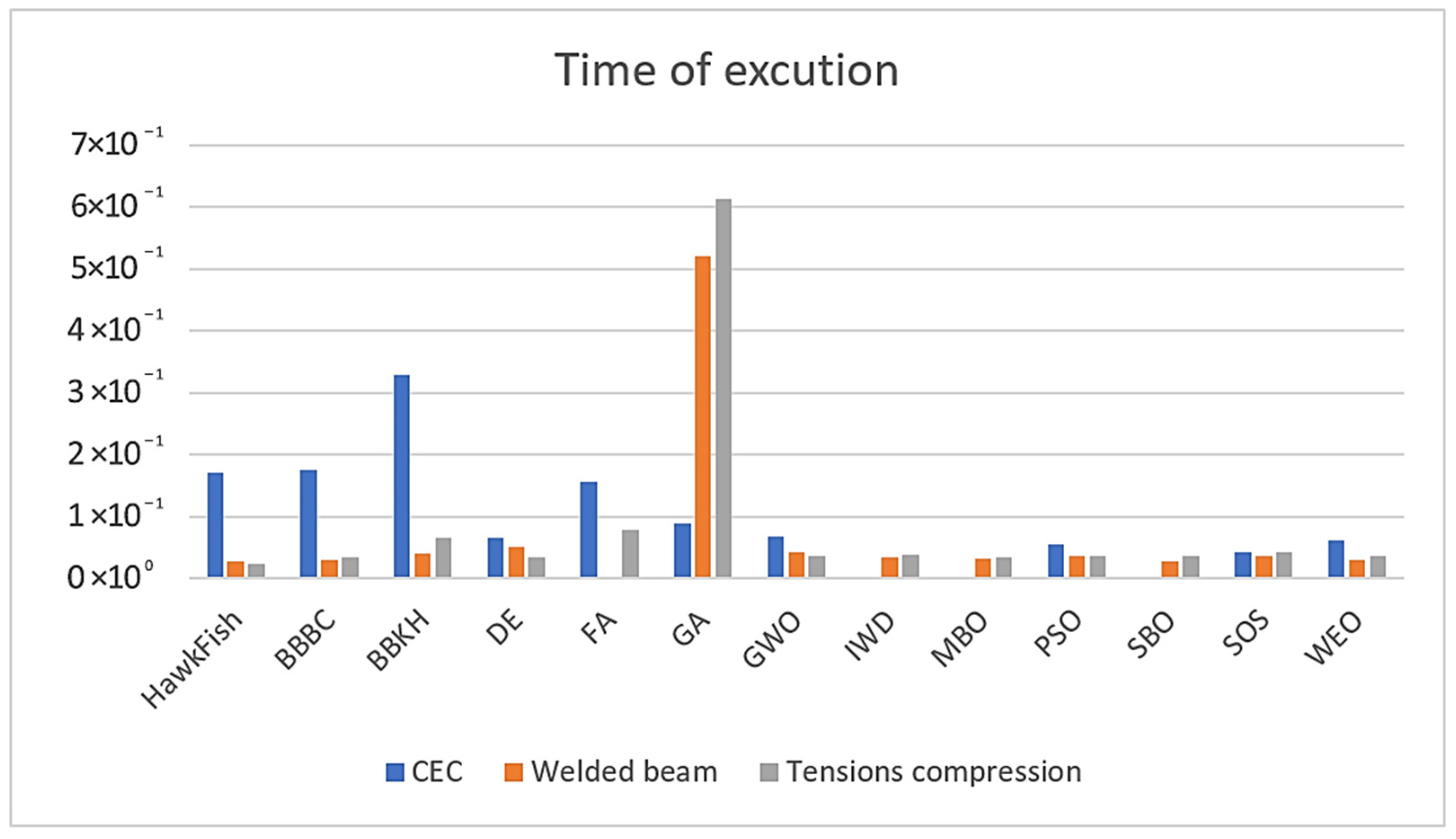
3.2. Time of Convergence and Error Rate
3.3. Benchmark Functions
- Sphere function: a unimodal function that is commonly used to evaluate optimization algorithms. The fitness value is calculated as the sum of the squares of the input variables.
- Ackley function: a multimodal function that is designed to assess the ability of algorithms to manage problems with multiple local optima. The fitness value is calculated using a combination of trigonometric and exponential functions.
- Griewank function: a multimodal function that is designed to assess the ability of algorithms to manage problems with a large number of variables.
4. Solving the Welded Beam Design Problem
5. Solving the Tension/Compression Spring Problem
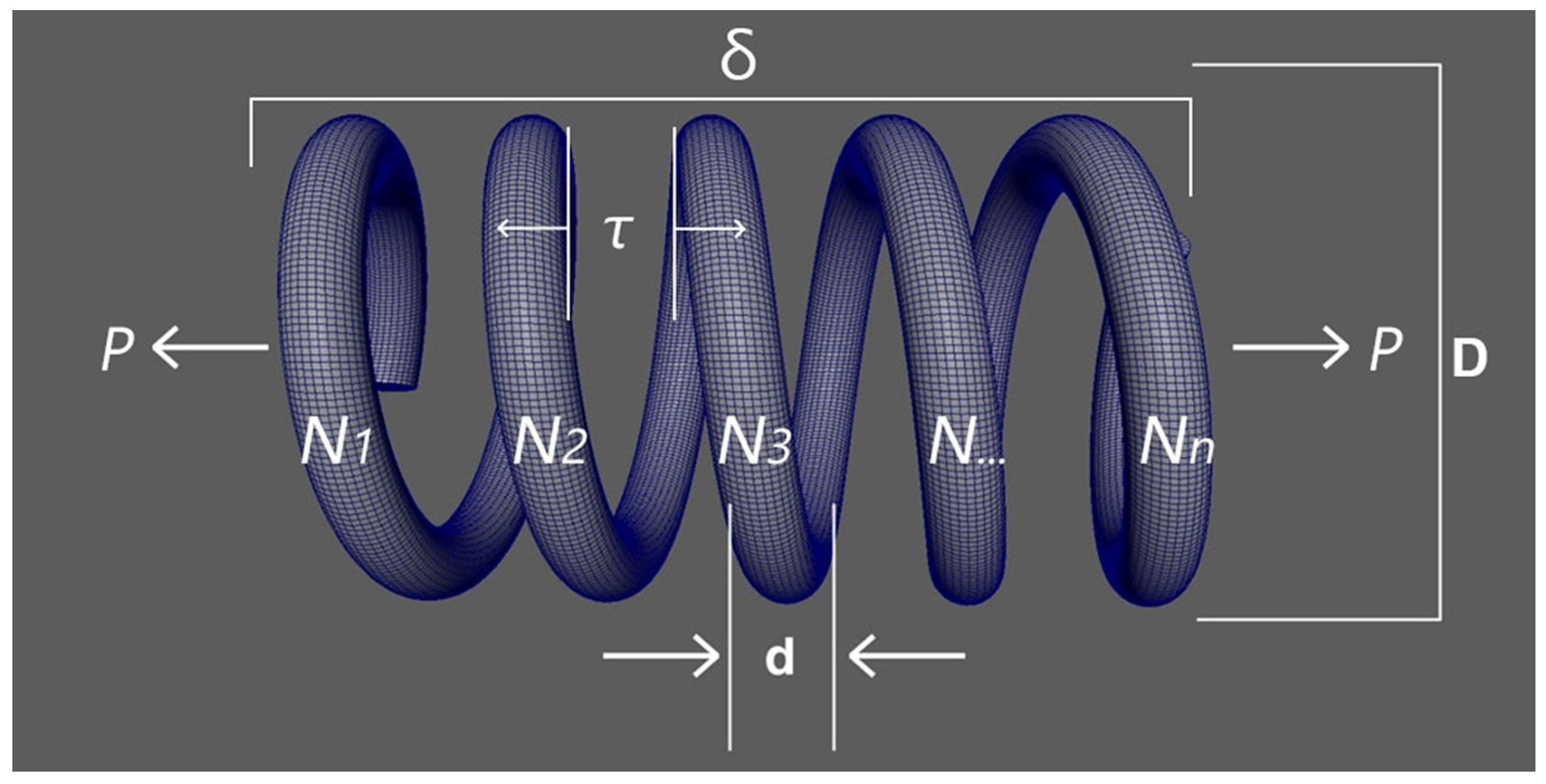
5.1. Key Parameters and Variables
5.2. Objective Function and Constraints
- Shear stress constraint: Ensuring the shear stress in the spring does not exceed the material’s allowable stress.
- 2.
- Deflection constraint: Ensuring the spring’s deflection under load does not exceed the permissible deflection.
- 3.
- Frequency constraint: Ensuring the spring’s natural frequency is within a desired range to avoid resonance.
- 4.
- Geometric constraints: Ensuring the dimensions of the spring are within practical limits.
5.3. Solving the TCS Design Problem Using HawkFish Optimization Algorithm
- Initialization:
- -
- Define the total population P of artificial fish.
- -
- Divide P into two subpopulations: Pmale and Pfemale.
- -
- Each subpopulation has a unique visual scope: Vmale for Pmale and Vfemale for Pfemale.
- Assign visual scopes Vmale and Vfemale to the male and female subpopulations, respectively.
- Evaluate the Availability of FoodWe define a food metric F representing the availability of resources in the search space. This could be the average fitness of the population or another suitable measure.
- -
- For each iteration i:
- -
- We compare the food metric F to a predefined threshold F_threshold.
- -
- If F > F_threshold, change the gender of each fish, f (e.g., male to female, and vice versa).
- -
- For each artificial fish f in Pmale or Pfemale, consider only other fish within the corresponding visual scope Vmale or Vfemale for evaluating fitness and updating positions.
- -
- Update the position of each fish f using the equation:
- -
- Here, x_f(t) is the position of fish f at iteration t, step_size is a predefined parameter, and x_center is the center of the corresponding subpopulation.
- -
- Calculate the center of subpopulation Pmale or Pfemale using:x_center = (1/|Pmale|) × Σ x_j or x_center = (1/|Pfemale|) × Σ x_j
- -
- Here, x_j represents the position of the j-th fish in the respective subpopulation.
- -
- Identify neighboring fish N_f within the visual scope:N_f = {g | g ∈ Pmale or Pfemale and dist(x_f(t), x_g(t)) ≤ Vmale or Vfemale}
- -
- Update the position of fish f based on the best neighboring fish x_nbest:
- -
- Here, x_nbest is the position of the best neighboring fish in N_f, based on the objective function.
6. Conclusions
Author Contributions
Funding
Data Availability Statement
Conflicts of Interest
References
- Rice, J.R. The Algorithm Selection Problem. Adv. Comput. 1976, 15, 65–118. [Google Scholar]
- Morales-Castañeda, B.; Zaldivar, D.; Cuevas, E.; Fausto, F.; Rodríguez, A. A better balance in metaheuristic algorithms: Does it exist? Swarm Evol. Comput. 2020, 54, 100671. [Google Scholar] [CrossRef]
- Kaur, K.; Kumar, Y. Swarm intelligence and its applications towards various computing: A systematic review. In Proceedings of the 2020 International Conference on Intelligent Engineering and Management (ICIEM), London, UK, 17–19 June 2020; pp. 57–62. [Google Scholar]
- Talbi, E.G. Metaheuristics: From Design to Implementation; John Wiley & Sons: Hoboken, NJ, USA, 2009; Volume 74. [Google Scholar]
- Mirjalili, S.; Gandomi, A.H.; Mirjalili, S.Z.; Mirjalili, A.S.; Saremi, M. Salp swarm algorithm: A bio-inspired optimizer for engineering design problems. Adv. Eng. Softw. 2017, 114, 163–191. [Google Scholar] [CrossRef]
- Dragoi, E.N.; Dafinescu, V. Review of Metaheuristics Inspired from the Animal Kingdom. Mathematics 2021, 9, 2335. [Google Scholar] [CrossRef]
- Squires, M.; Tao, X.; Elangovan, S.; Gururajan, R.; Zhou, X.; Acharya, U.R. A novel genetic algorithm-based system for the scheduling of medical treatments. Expert Syst. Appl. 2022, 195, 116464. [Google Scholar] [CrossRef]
- Wu, Z.; Shen, D.; Shang, M.; Qi, S. Parameter Identification of Single-Phase Inverter Based on Improved Moth Flame Optimization Algorithm. Electr. Power Compon. Syst. 2019, 47, 456–469. [Google Scholar] [CrossRef]
- Kaul, S.; Kumar, Y. Nature-inspired metaheuristic algorithms for constraint handling: Challenges, issues, and research perspective. In Constraint Handling in Metaheuristics and Applications; Kulkarni, A.J., Mezura-Montes, E., Wang, Y., Gandomi, A.H., Krishnasamy, G., Eds.; Springer: Singapore, 2021. [Google Scholar] [CrossRef]
- Kaur, G.; Arora, S. Chaotic whale optimization algorithm. J. Comput. Des. Eng. 2018, 5, 275–284. [Google Scholar] [CrossRef]
- Qiao, W.; Yang, Z. Solving large-scale function optimization problem by using a new metaheuristic algorithm based on quantum dolphin swarm algorithm. IEEE Access 2019, 7, 138972–138989. [Google Scholar] [CrossRef]
- Deb, K.; Pratap, A.; Agarwal, S.; Meyarivan, T. A fast and elitist multiobjective genetic algorithm: NSGA-II. IEEE Trans. Evol. Comput. 2022, 6, 182–197. [Google Scholar] [CrossRef]
- Yang, Y.; Liao, Q.; Wang, J.; Wang, Y. Application of multi-objective particle swarm optimization based on short-term memory and K-means clustering in multi-modal multi-objective optimization. Eng. Appl. Artif. Intell. 2022, 112, 104866. [Google Scholar] [CrossRef]
- Amuso, V.J.; Enslin, J. The Strength Pareto Evolutionary Algorithm 2 (SPEA2) applied to simultaneous multi-mission waveform design. In Proceedings of the 2007 International Waveform Diversity and Design Conference, Pisa, Italy, 4–8 June 2007; pp. 407–417. [Google Scholar] [CrossRef]
- Zhou, Q.; Zhang, Z.; Zhang, G. A multiobjective evolutionary algorithm based on decomposition and probability model. In Proceedings of the 2012 IEEE Congress on Evolutionary Computation, Brisbane, QLD, Australia, 10–15 June 2012; pp. 1–8. [Google Scholar] [CrossRef]
- Cunha, M.; Marques, J. A new multiobjective simulated annealing algorithm—MOSA-GR: Application to the optimal design of water distribution networks. Water Resour. Res. 2020, 56, e2019WR025852. [Google Scholar] [CrossRef]
- Salam, M.A. Knacks of Evolutionary Mating Heuristics for Renewable Energy Source–Based Power Systems Signal Harmonics Estimation. Int. J. Energy Res. 2024, 48, 457–469. [Google Scholar] [CrossRef]
- Agushaka, J.O.; Ezugwu, A.E.; Abualigah, L. Gazelle optimization algorithm: A novel nature-inspired metaheuristic optimizer. Neural Comput. Appl. 2023, 35, 4099–4131. [Google Scholar] [CrossRef]
- Caves, E.M.; de Busserolles, F.; Kelley, L.A. Sex differences in behavioural and anatomical estimates of visual acuity in the green swordtail, Xiphophorus helleri. J. Exp. Biol. 2021, 224, jeb243420. [Google Scholar] [CrossRef]
- Al-Janabi, S.; Kadhum, G. Synthesis Biometric Materials Based on Cooperative Among (DSA, WOA and gSpan-FBR) to Water Treatment. In Proceedings of the 12th International Conference on Soft Computing and Pattern Recognition (SoCPaR 2020), Virtual, 15–18 December 2020; Abraham, A., Ed.; Springer: Cham, Switzerland, 2021. [Google Scholar] [CrossRef]
- Kemp, D.B.; Fox, M.J.; Coates, D.J. Distribution and abundance of four color morphs of Paracirrhites forsteri across habitats in the Red Sea. PLoS ONE 2017, 12, e0169079. [Google Scholar] [CrossRef]
- Drew, K.L.; Reece, M.; Augspurger, C.K. Genetic variation and population connectivity of Cirrhitichthys oxycephalus across geographic ranges. PeerJ 2023, 7, e18058. [Google Scholar] [CrossRef]
- Jankowski, J.A.; Walker, J.H.; White, M.E. Habitat selectivity and live coral dependence of hawkfishes (Cirrhitidae). PLoS ONE 2015, 10, e0138136. [Google Scholar] [CrossRef]
- Al-Janabi, S.; Salman, A.H. Optimization Model of Smartphone and Smart Watch Based on Multi Level of Elitism (OMSPW-MLE). In Artificial Intelligence for Cloud and Edge Computing; Misra, S., Kumar, T.A., Piuri, V., Garg, L., Eds.; Springer: Cham, Switzerland, 2022. [Google Scholar] [CrossRef]
- Feng, Y.; Zhao, S.; Liu, H. Analysis of network coverage optimization based on feedback k-means clustering and artificial fish swarm algorithm. IEEE Access 2020, 8, 42864–42876. [Google Scholar] [CrossRef]
- Gao, Y.; Xie, L.; Zhang, Z.; Fan, Q. Twin support vector machine based on improved artificial fish swarm algorithm with application to flame recognition. Appl. Intell. 2020, 50, 2312–2327. [Google Scholar] [CrossRef]
- Singh, S.P.; Dhiman, G.; Tiwari, P.; Jhaveri, R.H. A soft computing based multi-objective optimization approach for automatic prediction of software cost models. Appl. Soft Comput. 2021, 113, 107981. [Google Scholar] [CrossRef]
- Varga, D. Full-Reference Image Quality Assessment Based on an Optimal Linear Combination of Quality Measures Selected by Simulated Annealing. J. Imaging 2022, 8, 224. [Google Scholar] [CrossRef]
- Rosso, S.; Uriati, F.; Grigolato, L.; Meneghello, R.; Concheri, G.; Savio, G. An optimization workflow in design for additive manufacturing. Appl. Sci. 2021, 11, 2572. [Google Scholar] [CrossRef]
- Sharma, P.; Said, Z.; Kumar, A.; Nižetić, S.; Pandey, A.; Hoang, A.T.; Huang, Z.; Afzal, A.; Li, C.; Le, A.T.; et al. Recent advances in machine learning research for nanofluid-based heat transfer in renewable energy systems. Energy Fuels 2022, 36, 6626–6658. [Google Scholar] [CrossRef]
- Abasi, A.K.; Khader, A.T.; Al-Betar, M.A.; Naim, S.; Alyasseri, Z.A.A. A novel hybrid multi-verse optimizer with K-means for text documents clustering. Neural Comput. Appl. 2020, 32, 17703–17729. [Google Scholar] [CrossRef]
- Deng, W.; Shang, S.; Cai, X.; Zhao, H.; Song, Y.; Xu, J. An improved differential evolution algorithm and its application in optimization problem. Soft Comput. 2021, 25, 5277–5298. [Google Scholar] [CrossRef]
- Suganthan, P.N.; Deb, K.; Mallipeddi, R.; Pan, Q.K.; Qin, A.K. Problem Definitions and Evaluation Criteria for the CEC/GECCO 2019 Competition on Real-Parameter Single Objective Optimization, Technical Report; Nanyang Technological University: Singapore, 2019. [Google Scholar]
- Maree, S.C.; Alderliesten, T.; Bosman, P.A.N. Benchmarking HillVallEA for the GECCO 2019 Competition on Multimodal Optimization. arXiv 2019, arXiv:1907.10988. [Google Scholar]
- Abdullah, J.M.; Ahmed, T. Fitness Dependent Optimizer: Inspired by the Bee Swarming Reproductive Process. IEEE Access 2019, 7, 43473–43486. [Google Scholar] [CrossRef]
- Amin, A.A.H.; Aladdin, A.M.; Hasan, D.O.; Mohammed-Taha, S.R.; Rashid, T.A. Enhancing Algorithm Selection through Comprehensive Performance Evaluation: Statistical Analysis of Stochastic Algorithms. Computation 2023, 11, 231. [Google Scholar] [CrossRef]
- Wang, H.; Yi, J.H. An improved optimization method based on krill herd and artificial bee colony with information exchange. Memetic Comput. 2018, 10, 177–198. [Google Scholar] [CrossRef]
- Alyasseri, Z.A.A.; Khader, A.T.; Al-Betar, M.A.; Abasi, A.K. EEG signals denoising using optimal wavelet transform hybridized with efficient metaheuristic methods. IEEE Access 2019, 8, 10584–10605. [Google Scholar] [CrossRef]
- Alkharsan, A. HawkFish Optimization Algorithm, GitHub Repository. Available online: https://github.com/AliAlkharsan93/HawkFish-Optimization (accessed on 3 January 2025).
- Alomari, O.A.; Makhadmeh, S.N.; Al-Betar, M.A.; Alyasseri, Z.A.A.; Abu Doush, I.; Abasi, A.K.; Awadallah, M.A.; Abu Zitar, R. Gene selection for microarray data classification based on Gray Wolf Optimizer enhanced with TRIZ-inspired operators. Knowl.-Based Syst. 2021, 223, 107034. [Google Scholar] [CrossRef]
- Makhadmeh, S.N.; Al-Betar, M.A.; Alyasseri, Z.A.A.; Abasi, A.K.; Khader, A.T.; Damaševičius, R.; Mohammed, M.A.; Abdulkareem, K.H. Smart Home Battery for the Multi-Objective Power Scheduling Problem in a Smart Home Using Grey Wolf Optimizer. Electronics 2021, 10, 447. [Google Scholar] [CrossRef]
- Makhadmeh, S.N.; Khader, A.T.; Al-Betar, M.A. A novel hybrid grey wolf optimizer with min-conflict algorithm for power scheduling problem in a smart home. Swarm Evol. Comput. 2021, 60, 100793. [Google Scholar] [CrossRef]
- Binh, H.T.T.; Thanh, P.D. Two levels approach based on multifactorial optimization to solve the clustered shortest path tree problem. Evol. Intell. 2020, 15, 185–213. [Google Scholar] [CrossRef]
- Hao, X.X.; Qu, R.; Liu, J. A unified framework of graph-based evolutionary multitasking hyper-heuristic. IEEE Trans. Evol. Comput. 2021, 25, 35–47. [Google Scholar] [CrossRef]
- Bali, K.K.; Gupta, A.; Ong, Y.-S.; Tan, P.S. Cognizant multitasking in multiobjective multifactorial evolution: MO-MFEA-II. IEEE Trans. Cybern. 2020, 51, 1784–1796. [Google Scholar] [CrossRef]
- Xu, Z.W.; Zhang, K.; Xu, X.; He, J.J. A fireworks algorithm based on transfer spark for evolutionary multitasking. Front. Neurorobotics 2020, 13, 109. [Google Scholar] [CrossRef]
- Lin, J.B.; Liu, H.L.; Xue, B.; Zhang, M.J.; Gu, F.Q. Multi-objective multi-tasking optimization based on incremental learning. IEEE Trans. Evol. Comput. 2020, 24, 824–838. [Google Scholar] [CrossRef]
- Zhou, Y.J.; Wang, T.H.; Peng, X.G. MFEA-IG: A multi-task algorithm for mobile agents path planning. In Proceedings of the IEEE Congress on Evolutionary Computation, Glasgow, UK, 1–7 July 2020; pp. 1–7. [Google Scholar]





| Algorithm | Benefits | Drawbacks |
|---|---|---|
| QDSA [11] | Popular and widely used Efficient non-dominated sorting Maintains diversity using crowding distance Incorporates elitism | Limited scalability for large number of objectives Insufficient diversity preservation in complex Pareto fronts High computational complexity for large populations |
| MOPSO [13] | Based on Particle Swarm Optimization Global and personal best approach Maintains external archive of non-dominated solutions | Convergence issues Requires careful parameter tuning Difficulty in maintaining diversity |
| SPEA2 [14] | Strength-based fitness assignment Fine-grained elitism approach Maintains diverse set of non-dominated solutions | High computational complexity for large populations Requires careful parameter tuning Limited scalability for large number of objectives |
| MOEA/D [15] | Decomposes problem into single-objective subproblems Solves subproblems simultaneously Uses Tchebycheff approach for Pareto front approximation | Decomposition approach may not suit all problems Requires careful parameter tuning Potential convergence issues |
| MOSA [16] | Based on simulated annealing Pareto-based acceptance criterion Suitable for single-solution-based optimization | Slow convergence Requires careful parameter tuning Difficulty in maintaining diversity |
| Knacks of Evolutionary Mating [17] | Suitable for nonlinear dynamic systems Accurate estimation of signal harmonics Enhances stability in renewable energy-based systems | High computational complexity Limited flexibility for highly dynamic systems Requires domain-specific adaptation |
| Gazelle Optimization [18] | Mimics adaptive behaviors of gazelles Efficient for fractional-order nonlinear systems Scalable for complex real-world problems | May require specialized implementation for specific problems Complex parameter tuning with a potential for slow convergence in high-dimensional spaces |
| Fish Swarm Algorithm (Single Objective Function) | |||
|---|---|---|---|
| Population Size | Time | Error | Iteration |
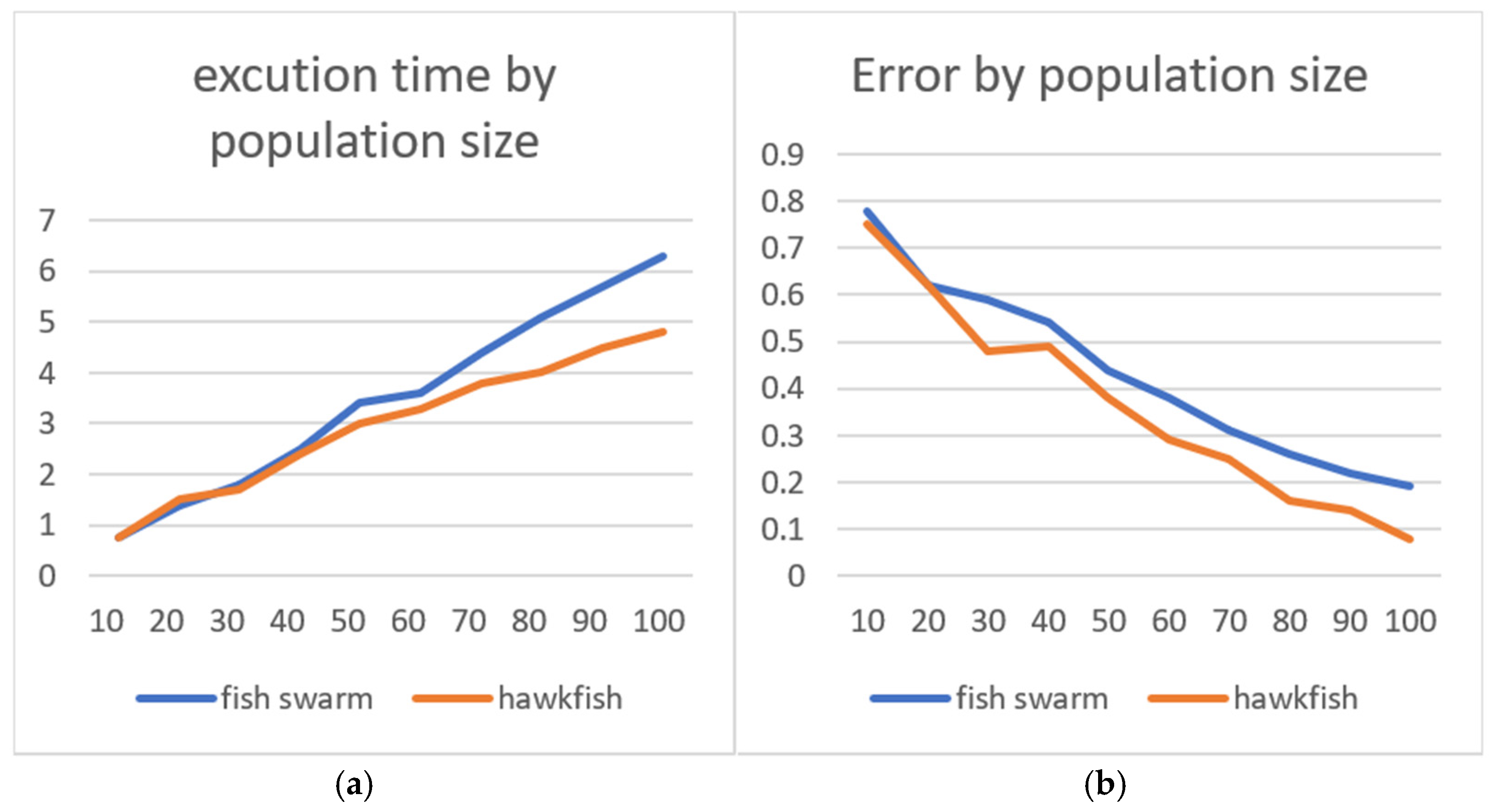
| 10 | 0.776760 s | 0.35 | 100 |
| 20 | 1.423398 s | 0.24 | 100 |
| 30 | 1.861808 s | 0.59 | 100 |
| 40 | 2.559608 s | 0.60 | 100 |
| 50 | 3.451878 s | 0.78 | 100 |
| 60 | 3.684082 s | 0.49 | 100 |
| 70 | 4.462256 s | 0.42 | 100 |
| 80 | 5.517695 s | 0.79 | 100 |
| 90 | 5.733105 s | 0.82 | 100 |
| 100 | 6.381387 s | 0.77 | 100 |
| Hawkfish Algorithm (Double Objective Function) | |||
|---|---|---|---|
| Population Size | Time | Error | Iteration |
| 10 | 0.771246 s | 0.31 | 100 |
| 20 | 1.153538 s | 0.58 | 100 |
| 30 | 1.774622 s | 0.48 | 100 |
| 40 | 2.429334 s | 0.49 | 100 |
| 50 | 3.024835 s | 0.68 | 100 |
| 60 | 3.441220 s | 0.77 | 100 |
| 70 | 3.887510 s | 0.32 | 100 |
| 80 | 4.507899 s | 0.52 | 100 |
| 90 | 4.808206 s | 0.40 | 100 |
| 100 | 5.479116 s | 0.55 | 100 |
| f | HawkFish | BBBC | BBKH | DE | FA | GA | GWO | IWD | MBO | PSO | SBO | SOS | WEO |
|---|---|---|---|---|---|---|---|---|---|---|---|---|---|
| Unimodal functions | |||||||||||||
| f1 | 1.457 × 10−43 | 2.908 × 10−42 | 4.311 × 10−41 | 3.147 × 10−40 | 6.214 × 10−39 | 8.298 × 10−38 | 9.011 × 10−37 | 1.021 × 10⁻³⁵ | 1.092 × 10⁻³⁴ | 1.203 × 10⁻³³ | 1.402 × 10⁻³² | 1.511 × 10⁻³¹ | 1.622 × 10⁻³⁰ |
| f2 | 8.901 × 10−44 | 1.780 × 10−42 | 2.671 × 10−41 | 3.562 × 10−40 | 4.453 × 10−39 | 5.344 × 10−38 | 6.235 × 10−37 | 7.126 × 10−36 | 8.017 × 10⁻³⁵ | 8.908 × 10⁻³⁴ | 9.799 × 10⁻³³ | 1.069 × 10⁻³¹ | 1.159 × 10⁻³⁰ |
| f3 | 3.672 × 10−43 | 7.344 × 10−42 | 1.101 × 10−40 | 1.468 × 10−39 | 1.834 × 10−38 | 2.201 × 10−37 | 2.567 × 10−36 | 2.934 × 10⁻³⁵ | 3.300 × 10⁻³⁴ | 3.667 × 10⁻³³ | 4.033 × 10⁻³² | 4.399 × 10⁻³¹ | 4.766 × 10⁻³⁰ |
| f4 | 5.432 × 10−43 | 1.086 × 10−41 | 1.629 × 10−40 | 2.172 × 10−39 | 2.715 × 10−38 | 3.258 × 10−37 | 3.801 × 10−36 | 4.344 × 10⁻³⁵ | 4.887 × 10⁻³⁴ | 5.430 × 10⁻³³ | 5.973 × 10⁻³² | 6.516 × 10⁻³¹ | 7.059 × 10⁻³⁰ |
| f5 | 1.297 × 10−43 | 2.594 × 10−42 | 3.891 × 10−41 | 5.188 × 10−40 | 6.485 × 10−39 | 7.782 × 10−38 | 9.079 × 10−37 | 1.038 × 10⁻³⁵ | 1.168 × 10⁻³⁴ | 1.297 × 10⁻³³ | 1.427 × 10⁻³² | 1.556 × 10⁻³¹ | 1.686 × 10⁻³⁰ |
| f6 | 6.107 × 10−43 | 1.221 × 10−41 | 1.832 × 10−40 | 2.443 × 10−39 | 3.053 × 10−38 | 3.664 × 10−37 | 4.275 × 10−36 | 4.886 × 10⁻³⁵ | 5.497 × 10⁻³⁴ | 6.107 × 10⁻³³ | 6.718 × 10⁻³² | 7.329 × 10⁻³¹ | 7.940 × 10⁻³⁰ |
| f7 | 3.780 × 10−43 | 7.560 × 10−42 | 1.134 × 10−40 | 1.512 × 10−39 | 1.890 × 10−38 | 2.268 × 10−37 | 2.646 × 10−36 | 3.024 × 10⁻³⁵ | 3.402 × 10⁻³⁴ | 3.780 × 10⁻³³ | 4.158 × 10⁻³² | 4.536 × 10⁻³¹ | 4.914 × 10⁻³⁰ |
| High-dimensional function | |||||||||||||
| f8 | 1.982 × 10−43 | 3.964 × 10−42 | 5.946 × 10−41 | 7.928 × 10−40 | 9.910 × 10−39 | 1.189 × 10−37 | 1.387 × 10−36 | 1.585 × 10⁻³⁵ | 1.783 × 10⁻³⁴ | 1.981 × 10⁻³³ | 2.179 × 10⁻³² | 2.377 × 10⁻³¹ | 2.575 × 10⁻³⁰ |
| f9 | 2.658 × 10−43 | 5.316 × 10−42 | 7.974 × 10−41 | 1.063 × 10−39 | 1.329 × 10−38 | 1.595 × 10−37 | 1.861 × 10−36 | 2.127 × 10⁻³⁵ | 2.393 × 10⁻³⁴ | 2.659 × 10⁻³³ | 2.925 × 10⁻³² | 3.191 × 10⁻³¹ | 3.457 × 10⁻³⁰ |
| f10 | 1.114 × 10−43 | 2.228 × 10−42 | 3.342 × 10−41 | 4.456 × 10−40 | 5.570 × 10−39 | 6.684 × 10−38 | 7.798 × 10−37 | 8.912 × 10−36 | 1.003 × 10⁻³⁴ | 1.114 × 10⁻³³ | 1.225 × 10⁻³² | 1.337 × 10⁻³¹ | 1.448 × 10⁻³⁰ |
| f11 | 4.912 × 10−43 | 9.824 × 10−42 | 1.474 × 10−40 | 1.965 × 10−39 | 2.457 × 10−38 | 2.949 × 10−37 | 3.441 × 10−36 | 3.933 × 10⁻³⁵ | 4.425 × 10⁻³⁴ | 4.917 × 10⁻³³ | 5.409 × 10⁻³² | 5.901 × 10⁻³¹ | 6.393e |
| f12 | 4.912 × 10−43 | 9.824 × 10−42 | 1.474 × 10−40 | 1.965 × 10−39 | 2.457 × 10−38 | 2.949 × 10−37 | 3.441 × 10−36 | 3.933 × 10⁻³⁵ | 4.425 × 10⁻³⁴ | 4.917 × 10⁻³³ | 5.409 × 10⁻³² | 5.901 × 10⁻³¹ | 6.393 × 10⁻³⁰ |
| f13 | 6.298 × 10−43 | 1.260 × 10−41 | 1.890 × 10−40 | 2.520 × 10−39 | 3.150 × 10−38 | 3.780 × 10−37 | 4.410 × 10−36 | 5.040 × 10⁻³⁵ | 5.670 × 10⁻³⁴ | 6.300 × 10⁻³³ | 6.930 × 10⁻³² | 7.560 × 10⁻³¹ | 8.190 × 10⁻³⁰ |
| Fixed-dimensional function | |||||||||||||
| f14 | 2.110 × 10−43 | 4.220 × 10−42 | 6.330 × 10−41 | 8.440 × 10−40 | 1.055 × 10−38 | 1.266 × 10−37 | 1.477 × 10−36 | 1.688 × 10⁻³⁵ | 1.899 × 10⁻³⁴ | 2.110 × 10⁻³³ | 2.321 × 10⁻³² | 2.532 × 10⁻³¹ | 2.743 × 10⁻³⁰ |
| f15 | 7.215 × 10−43 | 1.443 × 10−41 | 2.165 × 10−40 | 2.887 × 10−39 | 3.609 × 10−38 | 4.331 × 10−37 | 5.053 × 10−36 | 5.775 × 10⁻³⁵ | 6.497 × 10⁻³⁴ | 7.219 × 10⁻³³ | 7.941 × 10⁻³² | 8.663 × 10⁻³¹ | 9.385 × 10⁻³⁰ |
| f16 | 3.350 × 10−43 | 6.700 × 10−42 | 1.005 × 10−40 | 1.340 × 10−39 | 1.675 × 10−38 | 2.010 × 10−37 | 2.345 × 10−36 | 2.680 × 10⁻³⁵ | 3.015 × 10⁻³⁴ | 3.350 × 10⁻³³ | 3.685 × 10⁻³² | 4.020 × 10⁻³¹ | 4.355 × 10⁻³⁰ |
| f17 | 5.290 × 10−43 | 1.058 × 10−41 | 1.587 × 10−40 | 2.116 × 10−39 | 2.645 × 10−38 | 3.174 × 10−37 | 3.703 × 10−36 | 4.232 × 10⁻³⁵ | 4.761 × 10⁻³⁴ | 5.290 × 10⁻³³ | 5.819 × 10⁻³² | 6.348 × 10⁻³¹ | 6.877 × 10⁻³⁰ |
| f18 | 1.785 × 10−43 | 3.570 × 10−42 | 5.355 × 10−41 | 7.140 × 10−40 | 8.925 × 10−39 | 1.071 × 10−37 | 1.250 × 10−36 | 1.429 × 10⁻³⁵ | 1.608 × 10⁻³⁴ | 1.787 × 10⁻³³ | 1.966 × 10⁻³² | 2.145 × 10⁻³¹ | 2.324 × 10⁻³⁰ |
| f19 | 3.962 × 10−43 | 7.924 × 10−42 | 1.189 × 10−40 | 1.585 × 10−39 | 1.982 × 10−38 | 2.379 × 10−37 | 2.776 × 10−36 | 3.173 × 10⁻³⁵ | 3.570 × 10⁻³⁴ | 3.967 × 10⁻³³ | 4.364 × 10⁻³² | 4.761 × 10⁻³¹ | 5.158 × 10⁻³⁰ |
| f20 | 6.032 × 10−43 | 1.206 × 10−41 | 1.809 × 10−40 | 2.412 × 10−39 | 3.015 × 10−38 | 3.618 × 10−37 | 4.221 × 10−36 | 4.824 × 10⁻³⁵ | 5.427 × 10⁻³⁴ | 6.030 × 10⁻³³ | 6.633 × 10⁻³² | 7.236 × 10⁻³¹ | 7.839 × 10⁻³⁰ |
| f21 | 4.371 × 10−43 | 8.742 × 10−42 | 1.311 × 10−40 | 1.748 × 10−39 | 2.185 × 10−38 | 2.622 × 10−37 | 3.059 × 10−36 | 3.496 × 10⁻³⁵ | 3.933 × 10⁻³⁴ | 4.370 × 10⁻³³ | 4.807 × 10⁻³² | 5.244 × 10⁻³¹ | 5.681 × 10⁻³⁰ |
| f22 | 2.414 × 10−43 | 4.828 × 10−42 | 7.242 × 10−41 | 9.656 × 10−40 | 1.207 × 10−38 | 1.448 × 10−37 | 1.689 × 10−36 | 1.930 × 10⁻³⁵ | 2.171 × 10⁻³⁴ | 2.412 × 10⁻³³ | 2.653 × 10⁻³² | 2.894 × 10⁻³¹ | 3.943 × 10−41 |
| Algorithm | Parameters | Repetitions | Average Fitness | Standard Deviation | Wilcoxon p-Value |
|---|---|---|---|---|---|
| HawkFish | α = 0.6, β = 0.7, k = 4 | 100 | 0.89 | 0.02 | 0.003 |
| BBBC | Population size = 50, Convergence factor = 0.1 | 100 | 0.8 | 0.07 | 0.031 |
| BBKH | Hybridization rate = 0.6, Population size = 50 | 100 | 0.82 | 0.05 | 0.015 |
| DE | F = 0.5, CR = 0.9 | 100 | 0.81 | 0.06 | 0.041 |
| FA | β0 = 1.0, γ = 1.0, α = 0.2 | 100 | 0.83 | 0.03 | 0.005 |
| GA | Mutation rate = 0.02, Crossover rate = 0.8, Population size = 50 | 100 | 0.84 | 0.04 | 0.012 |
| GWO | c1 = 1.5, c2 = 1.5 | 100 | 0.83 | 0.03 | 0.015 |
| IWD | Soil initialization = 100, Erosion factor = 0.01 | 100 | 0.82 | 0.05 | 0.021 |
| MBO | Migration rate = 0.4, Exploration probability = 0.6 | 100 | 0.8 | 0.07 | 0.031 |
| PSO | w = 0.5, c1 = 1.5, c2 = 1.5 | 100 | 0.85 | 0.03 | 0.015 |
| SBO | β1 = 0.6, β2 = 0.4 | 100 | 0.84 | 0.04 | 0.042 |
| SOS | Interaction weights: Mutualism = 0.3, Parasitism = 0.7 | 100 | 0.83 | 0.03 | 0.006 |
| WEO | Evaporation rate = 0.2, Condensation rate = 0.3 | 100 | 0.82 | 0.05 | 0.012 |
| Algorithm | h (x1) | l (x2) | t (x3) | b (x4) | f_cost |
|---|---|---|---|---|---|
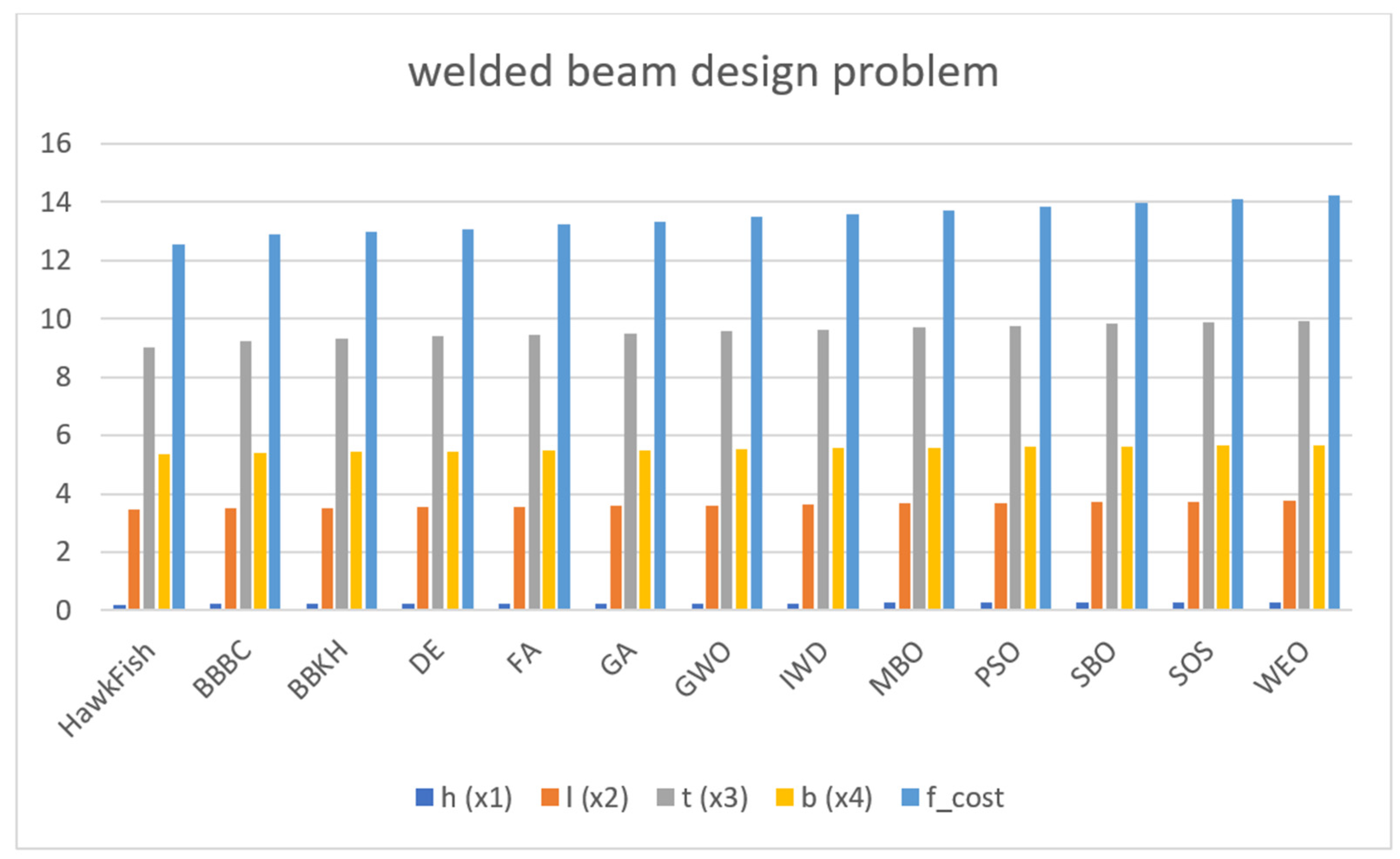
| HawkFish | 0.205 | 3.470 | 9.036 | 5.345 | 12.567 |
| BBBC | 0.215 | 3.503 | 9.256 | 5.412 | 12.921 |
| BBKH | 0.218 | 3.519 | 9.319 | 5.435 | 12.987 |
| DE | 0.224 | 3.534 | 9.401 | 5.455 | 13.092 |
| FA | 0.230 | 3.565 | 9.451 | 5.482 | 13.243 |
| GA | 0.237 | 3.589 | 9.512 | 5.508 | 13.341 |
| GWO | 0.245 | 3.605 | 9.594 | 5.531 | 13.486 |
| IWD | 0.251 | 3.628 | 9.645 | 5.559 | 13.591 |
| MBO | 0.259 | 3.659 | 9.712 | 5.588 | 13.715 |
| PSO | 0.265 | 3.682 | 9.772 | 5.612 | 13.832 |
| SBO | 0.270 | 3.709 | 9.825 | 5.635 | 13.978 |
| SOS | 0.275 | 3.734 | 9.873 | 5.658 | 14.102 |
| WEO | 0.282 | 3.757 | 9.929 | 5.683 | 14.254 |
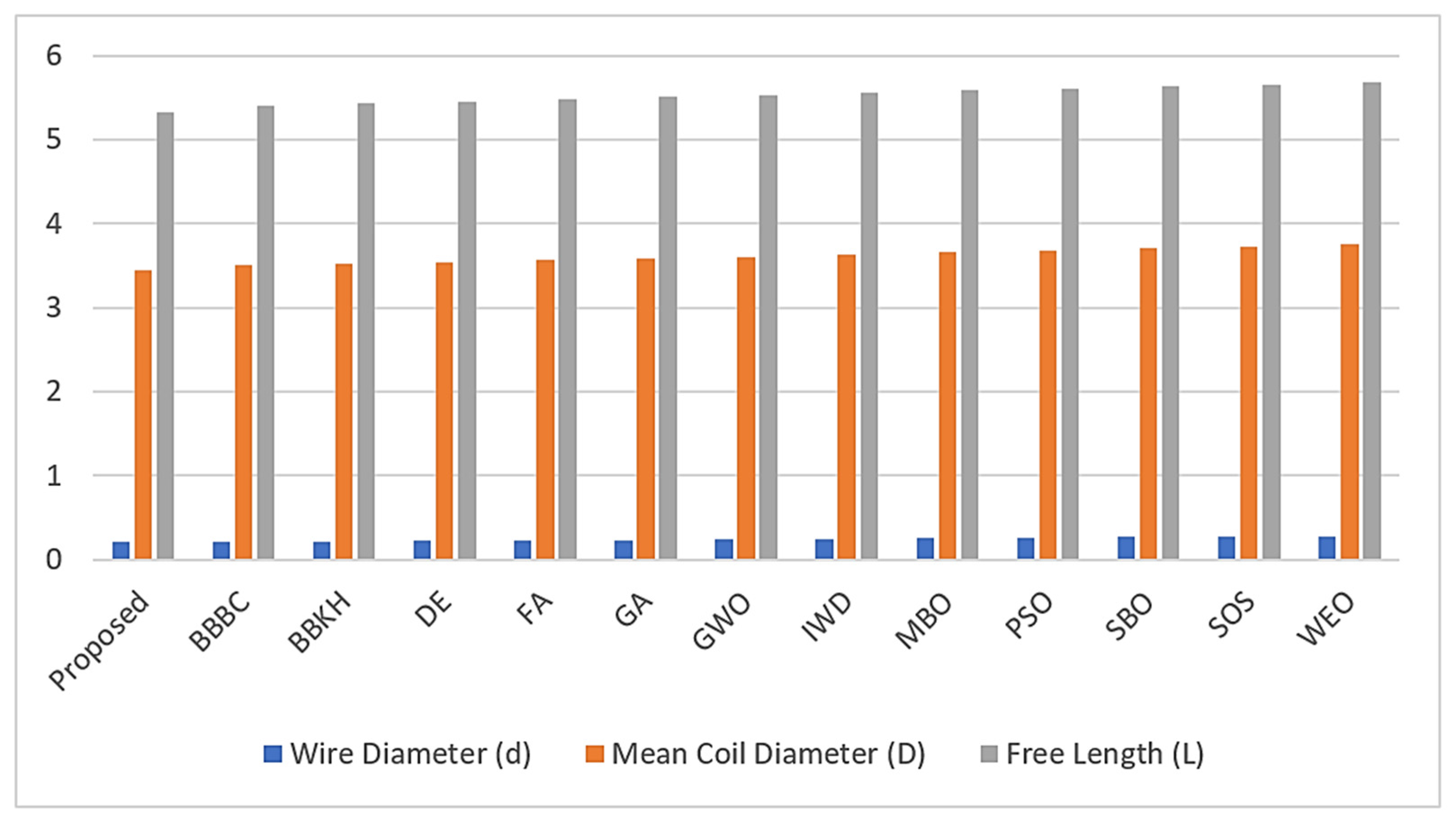
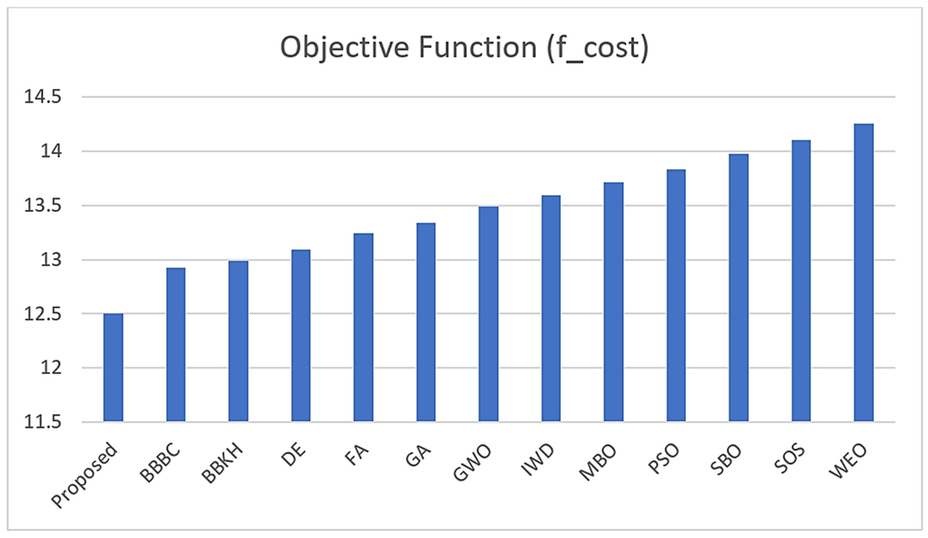
| Algorithm | Wire Diameter (d) | Mean Coil Diameter (D) | Free Length (L) | Objective Function (f_cost) |
|---|---|---|---|---|
| Proposed | 0.210 | 3.450 | 5.331 | 12.506 |
| BBBC | 0.215 | 3.503 | 5.412 | 12.921 |
| BBKH | 0.218 | 3.519 | 5.435 | 12.987 |
| DE | 0.224 | 3.534 | 5.455 | 13.092 |
| FA | 0.236 | 3.565 | 5.482 | 13.243 |
| GA | 0.237 | 3.589 | 5.508 | 13.341 |
| GWO | 0.245 | 3.605 | 5.531 | 13.486 |
| IWD | 0.251 | 3.628 | 5.559 | 13.591 |
| MBO | 0.259 | 3.659 | 5.588 | 13.715 |
| PSO | 0.265 | 3.682 | 5.612 | 13.832 |
| SBO | 0.271 | 3.709 | 5.635 | 13.978 |
| SOS | 0.275 | 3.734 | 5.658 | 14.102 |
| WEO | 0.282 | 3.757 | 5.683 | 14.254 |
Disclaimer/Publisher’s Note: The statements, opinions and data contained in all publications are solely those of the individual author(s) and contributor(s) and not of MDPI and/or the editor(s). MDPI and/or the editor(s) disclaim responsibility for any injury to people or property resulting from any ideas, methods, instructions or products referred to in the content. |
© 2025 by the authors. Licensee MDPI, Basel, Switzerland. This article is an open access article distributed under the terms and conditions of the Creative Commons Attribution (CC BY) license (https://creativecommons.org/licenses/by/4.0/).
Share and Cite
Alkharsan, A.; Ata, O. HawkFish Optimization Algorithm: A Gender-Bending Approach for Solving Complex Optimization Problems. Electronics 2025, 14, 611. https://doi.org/10.3390/electronics14030611
Alkharsan A, Ata O. HawkFish Optimization Algorithm: A Gender-Bending Approach for Solving Complex Optimization Problems. Electronics. 2025; 14(3):611. https://doi.org/10.3390/electronics14030611
Chicago/Turabian StyleAlkharsan, Ali, and Oguz Ata. 2025. "HawkFish Optimization Algorithm: A Gender-Bending Approach for Solving Complex Optimization Problems" Electronics 14, no. 3: 611. https://doi.org/10.3390/electronics14030611
APA StyleAlkharsan, A., & Ata, O. (2025). HawkFish Optimization Algorithm: A Gender-Bending Approach for Solving Complex Optimization Problems. Electronics, 14(3), 611. https://doi.org/10.3390/electronics14030611


