RAC-RTDETR: A Lightweight, Efficient Real-Time Small-Object Detection Algorithm for Steel Surface Defect Detection

Abstract

Steel, a fundamental material in modern industry, is widely used across manufacturing, construction, and energy sectors. Steel surface defects exhibit characteristics such as multiple classes, multi-scale features, small detection targets, and low-contrast backgrounds, making detection difficult. We propose RAC-RTDETR, a lightweight real-time detection algorithm designed for accurately identifying small surface defects on steel. Key improvements include: (1) The ARNet network, combining the ADown module and the RepNCSPELAN4-CAA module with a CAA-based attention mechanism, results in a lighter backbone network with better feature extraction and enhanced small-object detection by integrating contextual information; (2) The novel AIFI-ASMD module, composed of Adaptive Sparse Self-Attention (ASSA), Spatially Enhanced Feedforward Network (SEFN), Multi-Cognitive Visual Adapter (Mona), and Dynamic Tanh (DyT), optimizes feature interactions at different scales, reduces noise interference, and improves spatial awareness and long-range dependency modeling for better detection of multi-scale objects; (3) The Converse2D upsampling module replaces traditional upsampling methods, preserving details and enhancing small-object recognition in low-contrast, sparse feature scenarios. Experimental results on the NEU-DET and GC10-DET datasets show that RAC-RTDETR outperforms baseline models with MAP improvements of 3.56% and 3.47%, a 36.18% reduction in Parameters, a 40.70% decrease in GFLOPs, and a 7.96% increase in FPS.

1. Introduction

Steel, as one of the key materials in modern industry, has a huge demand across various sectors such as manufacturing, construction, and energy, particularly in high-speed rail and heavy industry, where steel quality plays a critical role. However, during steel production, surface defects such as cracks, protrusions, and scratches may occur due to process technology and environmental factors [1]. These defects not only affect the appearance of steel products but also shorten their lifespan and may even lead to severe safety accidents. Therefore, surface defect detection during steel production and processing is essential. Traditional industrial fault detection methods mainly include manual inspection and machine learning approaches. While early manual inspection methods offered high accuracy, they were labor-intensive and heavily reliant on professional experience. In recent years, deep learning-based detection methods have become the mainstream technology in defect detection due to their excellent performance. These data-driven approaches are extensively applied across various manufacturing domains to enhance quality control and process monitoring. For instance, Chen et al. [2] demonstrated the efficacy of 1DCNN-LSTM models in predicting surface roughness during precision grinding, while Ge et al. [3] utilized broad learning systems to address data scarcity in predicting composite drilling performance. Similarly, Wu et al. [4] applied ResNet architectures to classify geometric features in electrical discharge machining, highlighting the versatility of deep learning in decoding complex industrial signals. Deep learning techniques can automatically learn and extract key features of steel defects by training on a large dataset of labeled samples, enabling accurate identification and detection of these defects. This approach not only improves detection accuracy but also reduces the need for human intervention, making steel quality inspection more efficient and reliable.

Deep learning-based detection algorithms can be broadly classified into two categories based on their processing flow: single-stage algorithms and two-stage algorithms. Single-stage algorithms, such as the YOLO (You Only Look Once) [5] series and SSD (Single Shot MultiBox Detector) [6], generally offer better efficiency. These algorithms can perform both object detection and localization in a single pass, with the result obtained after just one backward propagation. In contrast, two-stage algorithms first generate candidate regions, then use methods such as selective search to extract potential target areas, and finally classify and precisely localize these regions. The two-stage algorithms are primarily represented by R-CNN and Faster R-CNN [7]. Although two-stage algorithms offer high accuracy, their model inference is more complex, resulting in slower inference speeds and larger parameter sizes. Currently, both single-stage and two-stage detectors typically use Non-Maximum Suppression (NMS) as a post-processing step. However, optimizing NMS is challenging, and its lack of robustness negatively impacts the inference speed of the detector.

To address the limitations of single-stage algorithms in detecting complex defects, and the issues of large parameters, slow speed, and insufficient robustness in two-stage algorithms, this paper improves the RTDETR [8], a single-stage algorithm that does not require anchors or NMS. To enhance the performance of both single-stage and two-stage algorithms, the modified RTDETR algorithm is named RAC-RTDETR. Test results on the NEU-DET and GC10-DET datasets show that the improved RAC-RTDETR algorithm outperforms the baseline algorithms in terms of detection accuracy, fewer parameters and computations, and faster inference speed, thus meeting the requirements of industrial applications. In summary, the contributions of the RAC-RTDETR algorithm are as follows:

• The ARNet backbone network is a lightweight architecture designed to reduce the impact of noise on model detection performance, significantly enhancing its ability to identify small targets. Compared to the baseline model, ARNet improves detection accuracy while reducing the model’s parameter count by 48.24%.
• A novel AIFI-ASMD module is developed to enhance the model’s ability to interact with features across different scales, improving spatial awareness and long-range dependency modeling.This results in improved detection performance for multi-scale objects. Experimental results on the NEU-DET dataset [9] show that incorporating this module boosts the model’s MAP by 1.58%.
• The Converse2D upsampling module is introduced to replace traditional upsampling methods. By reconstructing the input feature map, it preserves more detailed feature information, enhancing the model’s ability to detect small objects in low-contrast and feature-sparse scenarios. Experimental results show that the incorporation of this module improves the model’s MAP by 0.41%.
• Extensive experiments were conducted on the NEU-DET and GC10-DET datasets [10] using RAC-RTDETR.The experimental results show that, on the NEU-DET dataset, compared with the baseline model, RAC-RTDETR achieved improvements of 3.56% in MAP and 7.96% in FPS, while reducing the number of model parameters and GFLOPs by 36.18% and 40.70%, respectively.On the GC10-DET dataset, the MAP of RAC-RTDETR increased by 3.47%.

The rest of the paper is organized as follows: Section 2 summarizes related work; Section 3 presents the baseline model and the specific improvements made in this paper; Section 4 introduces the experimental setup; Section 5 discusses and analyzes the experimental results; Section 6 provides the conclusion of the proposed model.

2. Related Works

In this section, the related work on steel surface defect detection algorithms is introduced and summarized, primarily focusing on traditional methods and deep learning-based approaches.

Traditional methods mainly include manual visual inspection and machine learning approaches. Manual inspection suffers from low accuracy, low efficiency, and strong subjectivity. In traditional machine learning, data-driven industrial defect detection has proven effective. For example, Krummenacher et al. [11] developed a wavelet-based feature extraction method for time-series data and used a support vector machine for steel surface defect detection. However, traditional machine learning methods generally exhibit low recognition accuracy, making them insufficient for high-precision industrial applications.

With the continuous advancement of deep learning algorithms, deep learning-based methods for steel defect detection have rapidly evolved in terms of detection performance and generalization capabilities. These methods are classified into one-stage and two-stage algorithms. One-stage algorithms, such as SSD and YOLO, include the RAF-SSD algorithm proposed by Liu et al. [12], which integrates attention mechanisms and multi-feature fusion networks to improve detection accuracy by combining low- and high-level features. Liang et al. [13] introduced SDD-Net, which uses context enhancement and multi-scale feature fusion with a lightweight feature extraction network to ensure real-time detection. Lu et al. [14] developed FEP-YOLO, a lightweight method for resource-constrained devices, achieving good performance on limited devices through the use of a lightweight Faster R-CNN framework. Sun et al. [15] proposed CTL-YOLO, a lightweight algorithm for detecting defects in complex backgrounds, which incorporates a CGRCCFPN feature integration network for multi-scale global feature fusion, improving detection accuracy while maintaining a lightweight design. Liao et al. [16] introduced YOLOv10-based surface defect detection, enhancing feature extraction, fusion, and bounding box regression with the integration of the DualConv module, SlimFusionCSP module, and Shape-IoU loss function for improved accuracy. Two-stage algorithms, primarily based on R-CNN and Faster R-CNN, include Leng et al.’s [17] improved Faster R-CNN framework, which integrates feature fusion and lightweight channel attention mechanisms between FPN and RPN to enhance fine feature extraction. Gao et al. [18] proposed a Cascade R-CNN network using multi-head attention and dynamic loss reweighting, improving model robustness and detection accuracy. However, both one-stage and two-stage algorithms require confidence threshold filtering and Non-Maximum Suppression (NMS) during inference, resulting in slower speeds, larger parameter sizes, and redundancy issues in the computation process. To address this, end-to-end object detectors like RTDETR (DEtection TRansformer) have gained attention for their unique paradigm, which eliminates manual anchor boxes and NMS, using a bipartite graph matching strategy to directly establish a one-to-one correspondence between ground truth and predicted results, simplifying the detection process and improving performance. Mao et al. [19] proposed a lightweight steel defect detection algorithm based on RTDETR, incorporating depthwise separable convolutions (DWConv) and VoVGSCSP structures to refine feature fusion while reducing computational complexity. Su et al. [20] designed EL-DETR, a lightweight model using a Multi-Scale Fusion Attention (MFA) module for effective feature integration, significantly reducing parameters and computational load. Zhou et al. [21] introduced MESC-DETR, an improved RTDETR algorithm that uses a composite ConvNeXtV2 backbone and Dense High-Level Combination (DHLC) to enhance multi-scale feature extraction and edge information perception, improving detection accuracy.

Although the RTDETR-based steel surface defect detection algorithms mentioned above have shown promising performance, there are still areas for optimization: (1) Improving detection accuracy. (2) Reducing model parameters. (3) Reducing computational complexity. (4) Enhancing model detection speed.

3. Methods

In this section, the baseline model is first introduced, followed by a detailed explanation of the proposed RAC-RTDETR model and its three key improvements.

3.1. RTDETR Model

The RTDETR model consists of three main components: a backbone network, an efficient hybrid encoder, and a decoder with auxiliary prediction heads. The backbone network extracts multi-scale feature maps from input images through a series of convolutional layers. The hybrid encoder, which serves as the model’s core, includes two modules: Attention-based Intra-Scale Feature Interaction (AIFI) and Convolutional Neural Network-based Cross-Scale Feature Fusion (CCFM). AIFI enhances local feature representation, improves robustness, and reduces redundant computations of low-level features, thereby increasing efficiency. CCFM fuses features from multiple scales to strengthen detection capability across diverse scenarios. The Transformer [22] decoder further enhances global feature interaction through a self-attention mechanism, improving computational efficiency and detection performance in complex environments. RTDETR provides multiple variants, such as R18, R34, R50, R50m, R101, L, and X, to accommodate different detection needs. In this study, the lightweight RTDETR-R18 model, which has the smallest number of parameters, is selected as the baseline, as illustrated in Figure 1.

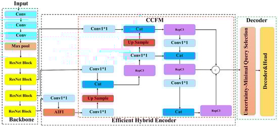
Figure 1. The structural diagram of the RTDETR-R18 model.

3.2. RAC-RTDETR Model

Although the baseline RTDETR model reduces inference latency and enhances detection speed by eliminating the need for post-processing (NMS) in real-time object detection, it still struggles with detection accuracy in complex backgrounds, challenges in detecting small objects, and high computational demands. To address these limitations, this paper proposes an improved RTDETR-based model, RAC-RTDETR. By modifying the backbone network, AIFI module, and upsampling module, RAC-RTDETR optimizes performance in four key areas: detection accuracy, detection speed, model parameter size, and computational complexity. The structure of RAC-RTDETR is shown in Figure 2.

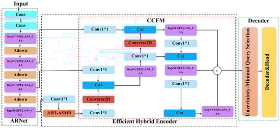
Figure 2. RAC-RTDETR Model structure diagram.

3.3. ARNet Backbone Network

In steel surface defect detection, some defects are very small. The RTDETR model’s feature extraction module uses max pooling and conventional convolutions, which can lead to information loss during feature extraction, amplifying the effect of noise and reducing detection accuracy for small defects. To address this, this paper adopts the RepNCSPELAN4 module from the YOLOv9 [23] and Context Anchor Attention mechanism (CAA) [24], combining them into a RepNCSPELAN4-CAA module. This is further integrated with the ADown (Adaptive Downsampling) module, resulting in the proposed ARNet backbone network, as shown in Figure 3.

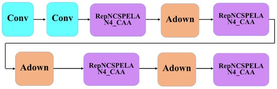
Figure 3. ARNet network structure diagram.

The RepNCSPELAN4-CAA module is composed of standard convolutions, RepNCSP, and the CAA attention mechanism, as shown in Figure 4. Initially, the input undergoes a convolution operation, followed by splitting it into two equal parts along the channel dimension. These parts then go through multi-path processing, where one path passes through the RepNCSP and convolution modules for feature extraction, and the resulting features from both paths are concatenated. Finally, the output is processed through the CAA attention mechanism and another convolution operation. RepNCSPELAN4-CAA is a lightweight module that combines the strengths of RepNCSPELAN4 and CAA attention, addressing issues such as model parameter redundancy and the lack of contextual relationships in original features. It provides stronger feature extraction capability and flexibility compared to traditional ResNet [25] blocks, making it more effective for capturing complex features.

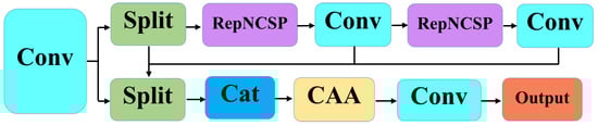
Figure 4. RepNCSPELAN4-CAA module structure diagram.

The CAA attention mechanism differs from classical attention mechanisms such as SE [26], CBAM [27], and ECA [28] by capturing contextual information and extracting long-range dependencies between pixels, while also enhancing central features. In CAA, average pooling is initially applied to minimize the impact of noise on detailed information.

$$F^{in}=Conv\left(P_{avg}\left(Input\right)\right)$$

(1)

Next, two DWConv (Depthwise Convolution) operations are applied to extract features.

$$F^{dw1}=DWConv\left(F^{in}\right)$$

(2)

$$F^{dw2}=DWConv\left(F^{dw1}\right)$$

(3)

DWConv consists of depthwise and pointwise convolutions, with the parameter count given by $DK \times DK \times M + M \times N$, where $DK$, M, and N represent the kernel size, the number of depthwise kernels, and the number of pointwise kernels, respectively. In contrast, the parameter count for a standard convolution is $DK \times DK \times X \times Y$, where $DK$, X, and Y represent the kernel size, input channels, and output channels, respectively. By setting the input and output channels X and Y equal to the number of depthwise kernels M and pointwise kernels N, the ratio of DWConv to standard convolution parameters is calculated as $\left({\displaystyle \frac{1}{N}}\right)+\left({\displaystyle \frac{1}{{\left(DK\right)}^2}}\right)$. Since N is typically large, the ${\displaystyle \frac{1}{N}}$ term can be ignored. Assuming the kernel size $DK$ is x, the parameters of depthwise separable convolution are approximately ${\displaystyle \frac{1}{x}}$ of those in standard convolution. By alternating between standard and depthwise separable convolutions, the module remains lightweight while effectively capturing spatial and channel features. Finally, a sigmoid function is applied to generate attention weights.

$$Output=Sigmoid\left(Conv\left(F^{dw2}\right)\right)$$

(4)

Additionally, we replace the downsampling convolution in the original backbone network with the ADown module. The ADown module is composed of average pooling, max pooling, and standard convolution, as illustrated in Figure 5.

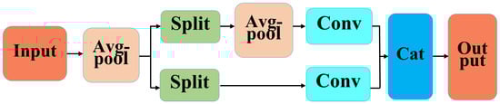
Figure 5. ADown module structure diagram.

The ADown module effectively reduces the parameter count and model complexity, enhancing computational efficiency, particularly in resource-constrained environments.

3.4. AIFI-ASMD Module

In the Transformer-based AIFI module, the traditional self-attention mechanism [22] has high computational cost and fails to effectively handle the internal scale interactions of fine-grained features. This issue limits the model’s performance in complicated scenarios, such as steel plate defect detection, where challenges like background noise, low contrast, and small detection targets occur. To address these, we propose a comprehensive improvement to the Transformer module, optimizing scale-internal feature interactions, reducing irrelevant noise, and lowering computational cost. The improved module is named AIFI-ASMD. The structures of the Transformer and AIFI-ASMD modules are shown in Figure 6.

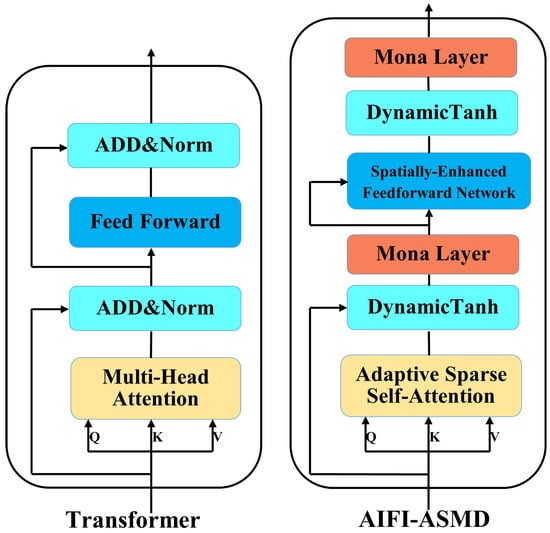
Figure 6. The structure diagram of the Transformer module and the structure diagram of the AIFI-ASMD module.

The AIFI-ASMD module comprises Adaptive Sparse Self-Attention (ASSA), Spatially Enhanced Feedforward Network (SEFN), Multi-Cognitive Visual Adapter (Mona), and the Dynamic Tanh (DyT) function.

3.4.1. The Adaptive Sparse Self-Attention (ASSA) Submodule

The traditional Transformer model, although capable of modeling long-range dependencies, often introduces redundant information and noise interactions, which degrade performance in detecting small targets on steel surfaces. To address these issues, we introduce Adaptive Sparse Self-Attention (ASSA). As shown in Figure 7, ASSA consists of two main branches: Sparse Self-Attention (SSA) and Dense Self-Attention (DSA), which are optimized through adaptive weighted fusion for feature aggregation.

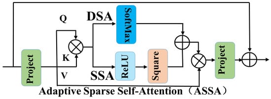
Figure 7. Adaptive Sparse Self-Attention (ASSA).

SSA achieves sparsity through a squared ReLU activation function, focusing only on features with high matching scores, thereby reducing the model’s attention to irrelevant information.

$$SSA=ReLU\left({\displaystyle \frac{Q{K}^T}{\sqrt{d}+B}}\right)$$

(5)

In the equation, Q and K represent the Query and Key, respectively; B is the learnable relative position bias; d is the model dimension; and ReLU is the activation function.

DSA, as a dense self-attention branch, ensures that the network captures interactions between all tokens, preserving all information that may be useful for predictions.

$$DSA=SoftMax\left({\displaystyle \frac{Q{K}^T}{\sqrt{d}+B}}\right)$$

(6)

In the equation, Q and K represent the Query and Key, respectively; B is the learnable relative position bias; d is the model dimension; and SoftMax is the activation function.

ASSA balances sparsity and information retention by adaptively combining the SSA and DSA branches. The model learns the weights of both branches to determine each branch’s contribution to the final output.

$$A=(w_1 \times \mathrm{SSA}+w_2 \times \mathrm{DSA}) \times V$$

(7)

In the equation, w1 and w2 are normalized weights used to adaptively adjust the contributions of SSA and DSA. V represents the value. The weights w1 and w2 regulate the weight calculation methods for sparse attention (SSA) and dense attention (DSA), with values between 0 and 1, and their sum equals 1, ensuring a balanced fusion of both branches’ outputs. This mechanism enables the model to learn, during training, how to adjust the relative importance of the two branches based on input features, allowing the model to better capture task-relevant features and improve performance.

$$w_n={\displaystyle \frac{e^{a_n}}{{\sum }_{i=1}^n{e}^{a_i}}},n=\{1,2\}$$

(8)

In the equation, n refers to the two different channels, DSA and SSA; w represents the normalized weight coefficient.

In summary, the ASSA module effectively captures complex dependencies in sequential data while maintaining computational efficiency. It reduces the model’s focus on irrelevant features and emphasizes the most useful information, thereby improving the model’s ability to detect detailed features and small objects.

3.4.2. The Spatially Enhanced Feedforward Network (SEFN) Submodule

Traditional feedforward modules often lack explicit modeling of spatial structures, making it difficult to capture the spatial and contextual relationships between different regions in an image. This issue becomes particularly challenging in the presence of complex occlusions or large missing areas, where feature generation is ineffective, leading to structural misalignment or blurred edges, thus hindering multi-scale small object detection. To overcome these challenges, we introduce the Spatially Enhanced Feedforward Network (SEFN), which effectively combines shallow spatial information with deep feature representations, enhancing the model’s ability to model spatial structures and maintain regional consistency. The structure of the SEFN module is shown in Figure 8.

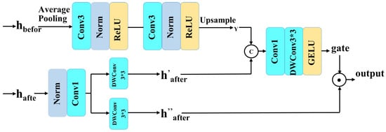
Figure 8. SEFN module structure diagram.

Specifically, the SEFN module first extracts $h_{\mathrm{before}}$ and $h_{\mathrm{after}}$ from the input feature map. $h_{\mathrm{before}}$ undergoes average pooling, two CONV3×3-Norm-ReLU operations, and upsampling to generate the spatially aware index Y, capturing the spatial relationships of $h_{\mathrm{before}}$. $h_{\mathrm{after}}$ is then split into $h_{\mathrm{after}}^{\prime }$ and $h_{\mathrm{after}}^{″}$, where $h_{\mathrm{after}}^{\prime }$ and Y undergo linear transformation and GELU non-linear activation to form a “gate.” This “gate” adjusts $h_{\mathrm{after}}^{″}$ by multiplication in elements, enhancing its spatial awareness. The entire process can be expressed by the following equation.

$$h_{after}^{\prime }=w_{d3}{w}_{1}LN\left(h_{after}\right)$$

(9)

$$h_{after}^{″}=w_{d3}{w}_{1}LN\left(h_{after}\right)$$

(10)

$$Y=Up\left(f\left(AveragePooling\left(h_{after}\right)\right)\right)$$

(11)

$$gate=GELU(w_{d3}{w}_{1}Y||h_{after}^{\prime })$$

(12)

$$Output=gate\odot h_{after}^{″}$$

(13)

In the equation, $w_1$ is a $1 \times 1$ convolution, and $w_{d3}$ is a $3 \times 3$ depthwise convolution, used for feature extraction and reducing computational cost. $LN$ represents layer normalization, f consists of two CONV–LN–ReLU operations, and $Up$ denotes an upsampling operation.

The SEFN module employs a three-stage strategy of “spatial extraction + guided gating + residual fusion” to construct a lightweight and effective spatial enhancement mechanism, significantly improving the model’s ability to perceive multi-scale small defects on steel surfaces under blurred background conditions.

3.4.3. The Multi-Cognitive Visual Adapter (Mona) Submodule

Despite the success of Transformer in visual and natural language tasks due to its powerful feature processing capabilities, it faces two main challenges in steel surface defect detection. First, the low contrast between defects and the background makes Transformer vulnerable to background noise, degrading detection performance. Second, the multi-scale and small nature of steel surface defects makes it difficult for the model to effectively identify small targets with significant scale variations.To address these challenges, this paper incorporates two layers of Mona into the module to enhance the model’s ability to handle multi-scale small targets in low-contrast backgrounds. This approach aligns with recent findings in electrochemical machining, where Wu et al. [29] demonstrated that integrating data-driven models with specific process parameters allows for the accurate real-time prediction of complex geometries and cavity profiles, effectively capturing the non-linear dynamics of the manufacturing process.

First, the Mona module adds two learnable weight parameters, $S_1$ and $S_2$, at the input and output of the LayerNorm (LN) layer to adjust the input distribution, enabling the filtering of background noise and enhancing task-relevant features.

$$x_{norm}=s_1{x}_{0}LN+s_2{x}_0$$

(14)

In the equation, $x_0$ represents the original input. Subsequently, Mona processes the input features from multiple perspectives, using depthwise convolutions (DWConv) with kernel sizes of $3 \times 3$, $5 \times 5$, and $7 \times 7$ to handle multi-scale small target features, adapting to the multi-scale nature of steel surface defects. A $1 \times 1$ convolution is then applied to aggregate the features, which are subsequently passed through a GeLU non-linearity. Finally, a projection reconstruction is performed to ensure that the output feature map has the same size as the input feature map.

$$x_{out}=x_0+U{G}_e\left(f_{dw1}\left(f_{dw3,5,7}\left(D\left(x_{norm}\right)\right)\right)\right)$$

(15)

In the equation, U and D represent upward and downward projections, $G_e$ denotes the GeLU activation, $f_{dw1}$ refers to a depthwise convolution with a $1 \times 1$ kernel, and $f_{dw3,5,7}$ represent depthwise convolutions with $3 \times 3$, $5 \times 5$, and $7 \times 7$ kernels, respectively.

3.4.4. The Dynamic Tanh (DyT) Function

The normalization layer is considered one of the fundamental components of modern neural networks, as it accelerates convergence and stabilizes training. In shallow LN layers, the input–output relationship is mostly linear, while in deeper layers, it becomes an S-shaped curve, as shown in Figure 9.

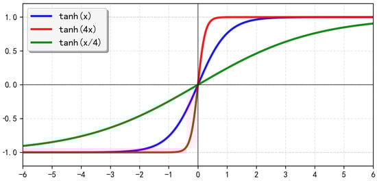
Figure 9. The curve of the Tanh function.

In this S-shaped curve, most points are concentrated in the central “linear region,” while other points outside this range fall into the “extreme region.” The main function of the normalization layer is to apply a “squeezing” effect to the outliers in the “extreme region,” compressing the main features of the data into a less extreme range.

As neural networks become more widespread and deeper, the necessity of normalization layers becomes even more critical, though at the cost of additional computational overhead. To improve the training and inference speed of the model, this paper introduces the Dynamic Tanh (DyT) function.

$$DyT\left(x\right)=\gamma \ast tanh\left(\alpha x\right)+\beta$$

(16)

In the equation, $\alpha$, $\gamma$, and $\beta$ are learnable parameters. DyT is not a new normalization layer, but it retains the “squeezing” effect on the values in the “extreme region” and the linear transformation operation on inputs in the “linear region.” The advantage of DyT lies in its ability to perform element-wise operations directly on vectors, eliminating the need to compute activation statistics during forward propagation, thereby improving the model’s inference speed.

3.5. Converse2D Module

Traditional upsampling methods use fixed interpolation rules, lacking flexibility and potentially losing critical detail information. To preserve more details and improve the model’s ability to recognize small targets, this paper introduces the Converse2D upsampling module as a replacement for traditional methods. The core idea of Converse2D is to formulate the deconvolution upsampling problem as a regularized least squares optimization. Given an input feature map $\mathbf{X}\in {\mathbb{R}}^{H \times W \times C}$ and a depthwise convolution kernel $\mathbf{K}\in {\mathbb{R}}^{k \times k \times C}$, the output $\mathbf{Y}$ after convolution with stride $s\ge 1$ is:

$$\mathbf{Y}={\mathcal{P}}_s(\mathbf{X};\mathbf{K})=\left(\mathbf{X}{\otimes }_d\mathbf{K}\right){\downarrow }_s$$

(17)

where ${\otimes }_d$ denotes depthwise convolution and ${\downarrow }_s$ denotes spatial subsampling. The inverse problem—recovering $\mathbf{X}$ from $\mathbf{Y}$, $\mathbf{K}$, and s—is ill-posed due to the non-invertible nature of the subsampling operation. To solve this, we formulate it as a regularized least-squares optimization problem. We seek the minimizer ${\mathbf{X}}^{\ast }$ of the objective function:

$$\mathcal{L}\left(\mathbf{X}\right)=\parallel \mathbf{Y}-\left(\mathbf{X}{\otimes }_d\mathbf{K}\right){\downarrow }_s{\parallel }_F^2+\lambda {\parallel \mathbf{X}-{\mathbf{X}}_0\parallel }_F^2$$

(18)

where the first term enforces data fidelity, the second is a Tikhonov regularization term with initial estimate ${\mathbf{X}}_0$ and strength $\lambda >0$, and ${\parallel ·\parallel }_F$ is the Frobenius norm. To derive an efficient closed-form solution, we adopt the circular boundary assumption, which allows us to leverage the convolution theorem and analyze the problem in the frequency domain. Let $\mathcal{F}(·)$ and ${\mathcal{F}}^{-1}(·)$ denote the 2D Discrete Fourier Transform (DFT) and its inverse, respectively. Under this assumption, the spatial subsampling operation has a specific representation in the frequency domain involving a folding and summation of frequency components.

A key step in the derivation is that the global minimization problem decouples into independent scalar sub-problems for each frequency component. For a given frequency coordinate (with indices omitted for clarity), the sub-problem is:

$$\underset{\widehat{x}}{min}\parallel \widehat{y}-\widehat{k}·\left(\widehat{x}{⊞}_s\right){\parallel }^2+\lambda {\parallel \widehat{x}-{\widehat{x}}_0\parallel }^2$$

(19)

where $\widehat{x}=\mathcal{F}\left(\mathbf{X}\right)$, $\widehat{k}=\overline{\mathcal{F}\left(\mathbf{K}\right)}$ (with $\overline{·}$ being complex conjugation), $\widehat{y}=\mathcal{F}\left(\mathbf{Y}{\uparrow }^s\right)$ is the DFT of the zero-upsampled $\mathbf{Y}$, and ${⊞}_s$ is an operator capturing the effect of stride-s subsampling in the frequency domain. Solving this by setting the complex gradient to zero yields the optimal frequency-domain solution for each component:

$${\widehat{x}}^{\ast }={\displaystyle \frac{\overline{\widehat{k}}{⊛}_s\widehat{y}+\lambda {\widehat{x}}_0}{\overline{\widehat{k}}{⊛}_s{\widehat{k}\parallel }_s+\lambda }}$$

(20)

Here, ${⊛}_s$ and ${\parallel }_s$ are stride-specific frequency-domain operators corresponding to stride-aware cross-correlation and auto-correlation, respectively. Reconstructing the spatial-domain solution via the inverse Fourier transform for all components defines the Converse2D operator:

$${\mathbf{X}}^{\ast }=\mathrm{Converse}2\mathrm{D}(\mathbf{Y},\mathbf{K},s;\lambda ,{\mathbf{X}}_0)={\mathcal{F}}^{-1}\left({\displaystyle \frac{\overline{\mathcal{F}\left(\mathbf{K}\right)}{⊛}_s\mathcal{F}\left(\mathbf{Y}{\uparrow }^s\right)+\lambda \mathcal{F}\left({\mathbf{X}}_0\right)}{\overline{\mathcal{F}\left(\mathbf{K}\right)}{⊛}_s{\mathcal{F}\left(\mathbf{K}\right)\parallel }_s+\lambda \mathbf{1}}}\right)$$

(21)

where $\mathbf{1}$ is an all-ones tensor. The derived operator possesses several critical properties: it provides an exact closed-form inverse under circular boundaries, its computational core based on FFTs is efficient with complexity $O(CHWlog(HW\left)\right)$, it is fully differentiable enabling end-to-end integration in neural networks, and its behavior can be tuned via $\lambda$ and ${\mathbf{X}}_0$. This rigorous formulation establishes Converse2D as a theoretically sound and practical module for feature reconstruction.

4. Experiment Setup

This section describes the experimental setup, which includes three aspects: the dataset, the experimental environment, and the evaluation metrics.

4.1. Datasets

The experiments in this paper use the NEU-DET dataset, released by Northeastern University, which contains 1800 grayscale images of typical surface defects in steel. These defects are categorized into six types: rolled-in scale, patches, crazing, pitted surface, inclusion, and scratches, with 300 images per category. The 1800 images are split into training, testing, and validation sets in an 8:1:1 ratio, i.e., 1440 images for training, 180 images for testing, and 180 images for validation. A subset of the NEU-DET dataset is shown in Figure 10.

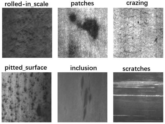
Figure 10. A subset of the NEU-DET dataset.

The generalization experiment in this paper is conducted on the GC10-DET dataset, which consists of 2293 images across 10 defect types: Punching (Pu), Welding Line (Wi), Crescent Gap (Cg), Water Spot (Ws), Oil Spot (Os), Silk Spot (Ss), Inclusion (In), Rolled Pit (Rp), Crease (Cr), and Waist Folding (Wf). The dataset is divided into training, testing, and validation sets in an 8:1:1 ratio. A subset of the GC10-DET dataset is shown in Figure 11.

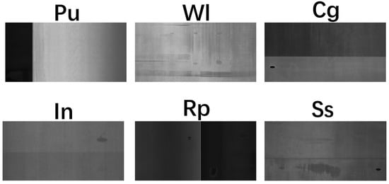
Figure 11. A subset of the GC10-DET dataset.

In addition, this paper also introduces a Welding defect detection dataset, which contains 6000 images, including four types of defects: Crack, Porosity, Spatters and welding-line. Unlike the NEU-DET and GC10-DET datasets, the detection targets of this dataset are larger, and some examples are shown in Figure 12.

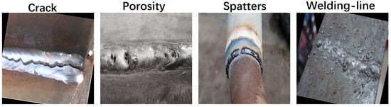
Figure 12. A subset of the Welding defect detection dataset.

4.2. Experimental Environment

The hardware environment for the experiments is as follows: GPU: NVIDIA GeForce RTX 4060 8GB, produced by TSMC in Taiwan, China, Processor: 12th Gen Intel(R) Core(TM) i5-12490F 3.00 GHz, produced by Intel in California, USA.The software environment includes Python 3.12, PyTorch 2.7.1, CUDA 12.6, and Windows 11. The basic experimental parameters are: epoch = 200, batch size = 16, workers = 0, learning rate (lr) = 0.01, optimizer = AdamW, momentum = 0.9.

4.3. Evaluation Metrics

The experimental results in this paper are evaluated using commonly used metrics in the field of object detection, including Mean Average Precision (MAP), GFLOPs, model parameters, and Frames Per Second (FPS). The formulas for these metrics are as follows.

$$P={\displaystyle \frac{TP}{TP+FP}}$$

(22)

$$R={\displaystyle \frac{TP}{TP+FN}}$$

(23)

$$AP={\int }_0^{1}P\left(R\right)dR$$

(24)

$$MAP={\displaystyle \frac{1}{N}}\sum _{i=1}^{N}A{P}_i$$

(25)

In the equation, $TP$ refers to True Positives, i.e., the targets correctly detected by the model; $FP$ refers to False Positives, which are negative samples incorrectly identified as targets by the model; $FN$ refers to False Negatives, which are actual targets that the model failed to detect. R measures the proportion of true positive samples out of all actual positive samples. $AP$ is calculated based on the Precision–Recall (P-R) curve, which depicts the relationship between precision and recall at different confidence thresholds. As the threshold increases, the model’s recall generally decreases while precision increases. $mAP$ is the mean Average Precision, which is the weighted average of $AP$ across all categories. It serves as a comprehensive metric to reflect the model’s performance across different classes, allowing for a more effective evaluation of overall model performance.

$$\mathrm{GFLOP}={\displaystyle \frac{\mathrm{Total}\mathrm{Floating}\mathrm{Point}\mathrm{Operations}}{{10}^9 \times \mathrm{Time}(\mathrm{in}\mathrm{seconds})}}$$

(26)

GFLOPs refers to the number of billion floating-point operations executed per second, and is a commonly used metric to measure the computational complexity of deep learning models.

$$\mathrm{Parameters}=\sum _{i=1}^L\left(\mathrm{Kernel}\mathrm{Height} \times \mathrm{Kernel}\mathrm{Width} \times \mathrm{Input}\mathrm{Channels}+1\right)\times \mathrm{Output}\mathrm{Channels}$$

(27)

The parameter count typically involves the sum of parameters from convolutional layers, fully connected layers, and other learnable parameters, and is used to reflect the size of the model.

$$FPS={\displaystyle \frac{\mathrm{frameNum}}{\mathrm{elapsedTime}}}$$

(28)

FPS is used to evaluate the detection speed of a model. It represents the number of images that can be processed per second and reflects the real-time detection capability of the model in practical applications.

5. Experimental Results and Analysis

In this section, we discuss and analyze the experimental results. Extensive experiments were conducted on the NEU-DET and GC10-DET datasets, including effectiveness experiments for the three improvements, comparison experiments, ablation studies, visual qualitative analysis, and generalization experiments. Except for the generalization experiments in Section 5.7, which were conducted on the GC10-DET dataset, all other experiments were performed on the NEU-DET dataset.

5.1. Effectiveness Experiment of the ARnet Backbone Network

To verify the effectiveness of the CAA attention mechanism in the ARnet backbone network, a comparison experiment was conducted on the NEU-DET dataset, involving various attention mechanisms, including SE, CBAM, ECA, and CAA. The experimental results are shown in Table 1.

Table 1. Comparison Results of Different Attention Mechanisms in the Backbone Network.

Methods	MAP/%	Parameters/M	GFLOPs	FPS/s
RepNCSPELAN	76.22	9.1	26.5	153
RepNCSPELAN-SE	76.13	9.4	34.4	156
RepNCSPELAN-CBAM	76.35	9.3	28.4	143
RepNCSPELAN-ECA	76.24	9.1	27.1	151
RepNCSPELAN-CAA (ARNet)	77.13	10.3	32.4	133

As shown in Table 1, there are certain differences in the impact of different attention mechanisms on model performance. The MAP without any attention mechanism is 76.22%. The introduction of the SE attention mechanism leads to a decrease in MAP. Using CBAM and ECA attention mechanisms results in an improvement in MAP compared to not using any attention mechanism, but they perform worse than the CAA attention mechanism. This indicates that CBAM, ECA, and CAA attention mechanisms all help enhance the backbone network’s ability to extract small targets. The CAA attention mechanism achieves the best MAP performance, reaching 77.13%. Although the CAA attention mechanism has lower performance in terms of Parameters, GPLOPs, and FPS compared to CBAM and ECA, the differences remain within an acceptable range. The CAA attention mechanism effectively balances MAP, Parameters, GPLOPs, and FPS.

We compared the MAP obtained by the Baseline and ARnet backbone networks for surface defects of steel in each category.

As shown in Figure 13, overall, ARnet achieves a 2.5% improvement in MAP compared to the Baseline, validating the effectiveness of ARnet. In terms of detection results for different types of defects, ARnet shows the largest MAP improvement for the inclusion and rolled-in scale categories, with improvements of 6.3% and 7.2%, respectively, indicating that ARnet enhances the model’s ability to detect small targets in low-contrast environments. Additionally, there are noticeable improvements for the crazing and pitted surface categories, further validating the effectiveness of ARnet. Although the MAP for the patches and scratches categories decreased, the drop is minimal and remains within an acceptable range.

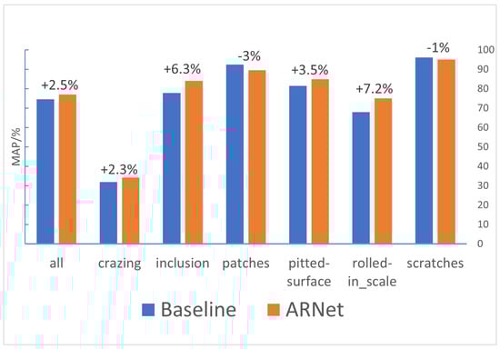
Figure 13. Comparison Results of MAP Obtained by Baseline and ARnet Backbone Networks for Surface Defects of Steel in Each Category.

5.2. Effectiveness Experiment of the AIFI-ASMD Module

To verify the effectiveness of the AIFI-ASMD module, this paper examines the impact of different components on model performance by sequentially adding various components. The specific operations are as follows: adding Adaptive Sparse Self-Attention (ASSA), adding Spatially Enhanced Feedforward Network (SEFN), adding Multi-cognitive Visual Adapter (Mona), and adding the Dynamic Tanh (DyT) function. The comparison results are shown in Table 2.

Table 2. Performance Comparison Results of Different Components in AIFI-ASMD.

Methods	MAP/%	Parameters/M	GFLOPs	FPS/s
ASSA	74.75	20.7	57.8	104
ASSA-SEFN	74.84	22.2	58.3	107
ASSA-SEFN-Mona	75.47	22.3	58.4	109
ASSA-SEFN-Mona-DyT (AIFI-ASMD)	76.18	22.3	58.4	111

As shown in Table 2, the MAP improves by sequentially adding ASSA, SFEN, Mona, and Tanh (DyT), indicating that each component contributes positively to the model’s performance. The ASSA-SEFN-Mona-DyT (AIFI-ASMD) module achieves the best MAP performance of 76.18% without increasing Parameters or GFLOPs, demonstrating that the module effectively balances detection accuracy and model lightweighting. Notably, by introducing the Dynamic Tanh (DyT) function, AIFI-ASMD performs excellently in FPS, reaching 111, indicating that the Dynamic Tanh (DyT) function helps to improve the model’s detection speed.

To deeply analyze the impact of each sub-module (ASSA, SEFN, Mona, DyT) on the model’s reasoning speed, we conducted a detailed examination of the reasoning time of each sub-module on each picture, as shown in Table 3.

Table 3. The reasoning time of each sub-module on each picture.

Methods	Preprocessing/ms	Postprocessing/ms	Reasoning/ms
ASSA	0.287	0.236	9.627
ASSA-SEFN	0.270	0.247	9.378
ASSA-SEFN-Mona	0.259	0.247	9.188
ASSA-SEFN-Mona-DyT	0.264	0.259	9.033

As shown in Table 3, the reasoning speed of the ASSA-SEFN-Mona-DyT (AIFI-ASMD) module is the fastest, and the time spent reasoning each picture is 9.033 milliseconds.

In deep learning, it is generally determined whether the training is stable by observing the loss function curve. We focused on observing the changes in the classification loss function curve when DyT was not introduced and when DYT was introduced, as shown in Figure 14.

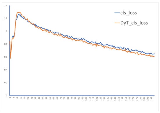
Figure 14. Classification Loss Function Curve.

By observing Figure 14, it can be seen that the classification loss function curves roughly overlap when DyT is not introduced and when DyT is introduced. After the introduction of DyT, the classification loss function curve does not show significant fluctuations, indicating that the model training after the introduction of DYT is relatively stable.

We performed attention visualization for the different components of the AIFI-ASMD module, as shown in Figure 15.

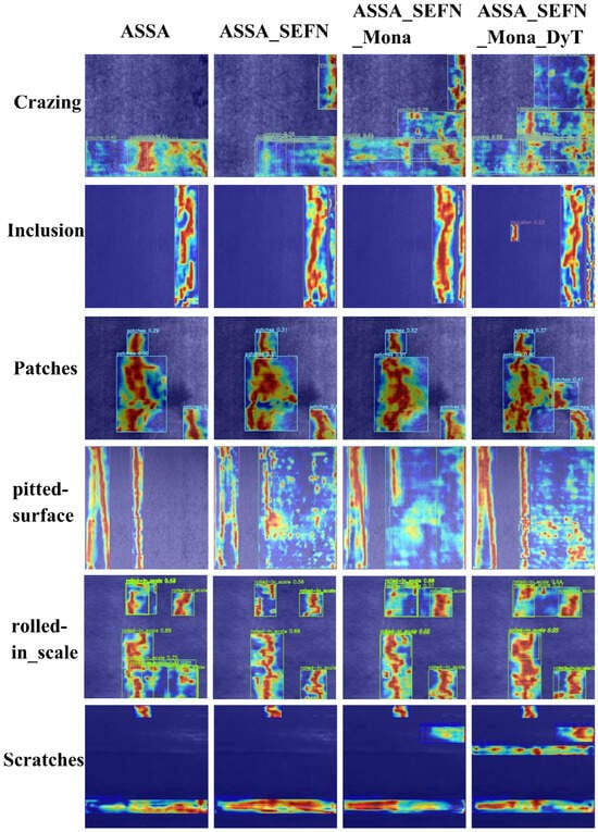
Figure 15. Attention Visualization Results of Different Components in the AIFI-ASMD Module.

As shown in Figure 15, the AIFI-ASMD module is able to accurately focus on defect regions in complex backgrounds, effectively attending to both small and multi-scale targets in the image. In contrast, other methods either struggle to attend to edge features or fail to capture small target characteristics, leading to attention misalignment. The visualization comparison results indicate that the AIFI-ASMD module demonstrates stronger recognition ability and robustness for multi-scale small target defects on steel surfaces.

5.3. Effectiveness Experiment of the Converse2D Module

To validate the effectiveness of the Converse2D module, this paper compares the nearest-neighbor interpolation (baseline model method), dynamic upsampling [30], and the upsampling method proposed in this paper (Converse2D). The comparison experimental results are shown in Table 4.

Table 4. Comparison Results of Different Upsampling Methods.

Methods	MAP/%	Parameters/M	GFLOPs	FPS/s
Nearest-Neighbor Interpolation (NNI)	74.60	19.9	57.0	113
Dynamic Upsampling (DU)	74.67	19.9	57.0	110
Converse2D	75.01	19.9	57.0	88

As shown in Table 4, the Parameters and GFLOPs for the three upsampling methods are almost identical. The baseline model method performs the best in FPS, while Converse2D also shows impressive FPS performance and achieves the highest MAP.

As shown in Figure 16, although the FPS performance of Converse2D is not the best, the gap compared with the baseline method is within an acceptable range. Considering the detection accuracy, Converse2D is chosen as the upsampling method for the model in this paper.

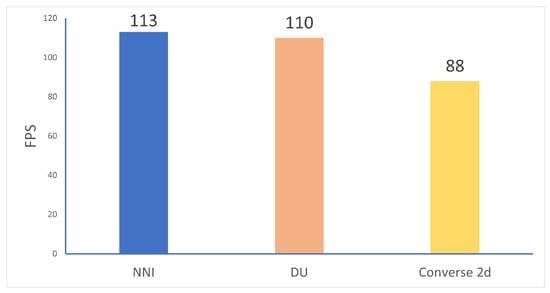
Figure 16. Comparison Results of FPS for Different Upsampling Methods.

5.4. Comparison Experiment

To comprehensively compare the detection performance of RAC-RTDETR and the baseline model, the comparison results across various metrics on the NEU-DET dataset are shown in Table 5, The resolution of the input images of the models in the comparison experiments is all 640 × 640. F1-Score represents the harmonic mean of Precision and Recall, MAP50-90 is the average MAP under the IoU threshold of 50–90.

Table 5. Comparison results of RAC-RTDETR and the baseline model on the NEU-DET dataset.

Baseline
Category	Precisoion/%	Recall/%	F1-Score/%	MAP/%	MAP50-90/%
crazing	65.57	17.60	27.72	31.94	12.51
inclusion	73.82	72.55	73.18	77.79	42.34
patches	83.32	90.27	86.66	92.50	60.34
pitted surface	75.63	72.19	73.87	81.43	47.60
rolled-in scale	70.45	71.67	71.05	67.88	30.13
scratches	82.28	94.87	88.43	96.07	59.72
all	75.27	69.86	70.16	74.60	42.27
RAC-RTDETR
crazing	70.49 (+4.92)	24.62 (+7.02)	36.49 (+8.74)	40.65 (+8.71)	17.65 (+5.14)
inclusion	77.26 (+3.44)	77.45 (+4.90)	77.36 (+4.18)	82.82 (+5.03)	46.81 (+4.47)
patches	79.79 (−3.53)	89.16 (−1.11)	84.21 (−2.45)	90.58 (−1.92)	60.50 (+0.16)
pitted surface	79.55 (+3.92)	76.74 (+4.55)	78.12 (+4.25)	84.04 (+2.61)	50.72 (+3.12)
rolled−in scale	70.37 (−0.08)	73.33 (+1.66)	71.82 (+0.77)	74.35 (+6.47)	36.88 (+5.75)
scratches	86.04 (+3.76)	94.88 (+0.01)	90.24 (+1.81)	96.52 (+0.45)	61.38 (+1.66)
all	77.25 (+1.98)	72.69 (+2.83)	73.04 (+2.88)	78.16 (+3.56)	45.66 (+3.39)

As shown in Table 5, RAC-RTDETR outperforms the baseline model in terms of Precision, Recall, F1-score, MAP50, and MAP50-90, with improvements of 1.98%, 2.86%, 3.56%, 3.39%, respectively, demonstrating superior detection accuracy and stability. In terms of defect categories, RAC-RTDETR achieves improvements across all five defect types—crazing, inclusion, pitted surface, rolled-in scale, and scratches—on all metrics, indicating its ability to effectively identify various surface defects in steel and its adaptability to real-world steel production environments. Although RAC-RTDETR shows a slight decrease in Precision, Recall, F1-score, and MAP50 for the patches class, it still performs well with values of 79.79%, 89.16%, 84.21%, and 90.58%, respectively, and shows a 0.16% improvement in MAP50-90, suggesting that its overall detection performance exceeds that of the baseline model.

Additionally, this paper compares the detection performance of RAC-RTDETR with currently popular object detection algorithms on the NEU-DET dataset. The comparison results are shown in Table 6.

Table 6. Results of the Performance Comparison Across Different Models.

Methods	MAP/%	Parameters/M	GFLOPs	FPS/s
Faster RCNN	74.81	28.4	94.12	51
Yolov5n	74.15	1.9	4.9	83
Yolov7-tiny	71.82	6.8	13.1	77
Yolov8n	76.55	3.1	8.1	96
Yolov10s	71.36	7.2	21.4	83
Yolo11n	76.13	2.58	6.3	92
RTDETR-R18 (Baseline)	74.60	19.9	57.0	113
RTDETR-R34	75.84	31.1	88.8	98
RTDETR-R50	75.99	41.9	129.6	62
RAC-RTDETR (ours)	78.16	12.7	33.8	122

As shown in Table 6, Faster RCNN algorithms achieve high detection accuracy, but their large model size and complexity make them unsuitable for edge device deployment. While the Yolo series algorithms offer lightweight and real-time performance, their detection accuracy is suboptimal. RTDETR-R34 and RTDETR-R50, as upgraded versions of RTDETR-R18, provide better accuracy than RTDETR-R18 but still fall short of the proposed RAC-RTDETR algorithm. Additionally, these models face challenges in deployment due to their large parameter size. In conclusion, RAC-RTDETR delivers the best detection accuracy while maintaining lightweight and real-time performance.

5.5. Ablation Experiment

In the experiments, the ablation experiment evaluates the contribution of specific modules by selecting and removing different modules or combinations of modules. Eight sets of ablation experiments were designed and conducted on the NEU-DET dataset. The results of the ablation experiment are presented in Table 7.

Table 7. Comparison Results of Ablation Experiment.

Methods	MAP/%	Parameters/M	GFLOPs	FPS/s
Baseline	74.60	19.9	57.0	113
ARNet	77.13	10.3	32.4	133
Converse2D	75.01	19.9	57.0	88
AIFI-ASMD	76.18	22.3	58.4	111
ARNet+AIFI-ASMD	75.74	12.7	33.8	119
ARNet+Converse2D	76.45	10.3	32.4	123
AIFI-ASMD + Converse2D	76.01	22.3	58.4	95
ARNet+AIFI-ASMD + Converse2D (ours)	78.16	12.7	33.8	122

As shown in Table 7, introducing the ARNet, Converse2D, and AIFI-ASMD modules individually leads to improvements in the model’s MAP, further validating the effectiveness of the proposed improvements. Among them, ARNet contributes the most to the model’s lightweight design, reducing the model’s parameter count by 48.42% compared to the baseline. ARNet module performs well in terms of inference speed, improving by 17.70% compared to the baseline. In subsequent experiments combining these modules in pairs, the model’s MAP, Parameters and GFLOPs all show varying degrees of improvement over the baseline. Finally, the combination of ARNet, Converse2D, and AIFI-ASMD in the proposed model achieves the optimal MAP performance of 78.16%, an improvement of 3.56%. Additionally, RAC-RTDETR reduces Parameters by 36.18%, GFLOPs by 40.70%, and increases FPS by 7.96% compared to the baseline. These results demonstrate that the proposed method effectively integrates the strengths of each module, maintaining excellent overall performance.

We present the precision–recall curves formed during the eight sets of ablation experiments, as shown in Figure 17.

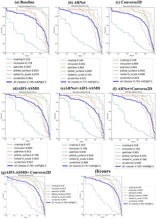
Figure 17. P-R curves for each set of ablation experiments.

From the P-R curves, it can be seen that the MAP of the crazing class reaches its highest value of 41.8% in the 6th set of ablation experiments, the inclusion class reaches 84.1% in the 2nd set, the pitted surface class achieves 85.9% in the 3rd set, the rolled-in scale class reaches 75.1% in the 2nd set, and the scratches class attains 98.8% in the 5th set. This indicates that the proposed improvements play a crucial role in enhancing the model’s detection capability. The 8th set of ablation experiments exhibits the best overall detection performance, further validating that RAC-RTDETR effectively integrates the advantages of each improvement, offering high detection capability for various types of surface defects in steel. It is worth noting that the model’s detection performance on the patches class slightly decreased by 1.9%, and improving the detection accuracy for this category will be one of the directions for future work.

5.6. Visual Qualitative Analysis Experiment

To visually demonstrate the superiority of RAC-RTDETR’s detection capability, the actual detection results and attention visualizations are compared with the baseline model. The comparison of detection results and attention visualizations are shown in Figure 18 and Figure 19.

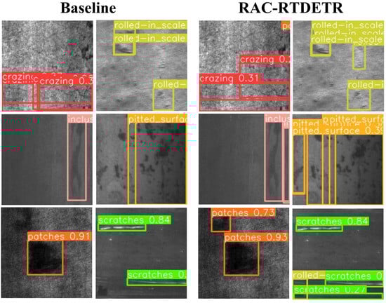
Figure 18. Comparison of actual detection results on the NEU-DET dataset.

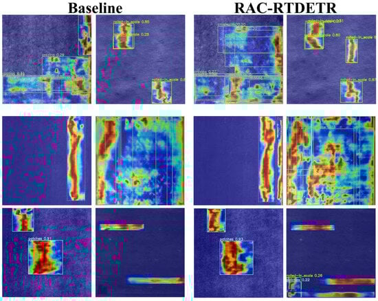
Figure 19. Comparison of attention visualization results on the NEU-DET dataset.

From the comparison of actual detection results, it can be seen that the baseline model fails to effectively detect defects such as crazing, rolled-in scale, and pitted surface due to their low contrast with the background and small target size. Additionally, the baseline model struggles to capture defects with significant scale variations, such as inclusion and scratches. However, the improved RAC-RTDETR effectively detects both small targets and targets with large scale variations.

From the comparison of attention visualizations, it can be seen that in the defect regions detected by both the baseline model and RAC-RTDETR, RAC-RTDETR shows darker colors, indicating that RAC-RTDETR focuses more attention on the defect areas compared to the baseline model, demonstrating stronger detection stability.

5.7. Generalization Experiment

We conducted generalization experiments on the GC10-DET dataset. The P-R curves of the baseline model and RAC-RTDETR on the GC10-DET dataset are shown in Figure 20.

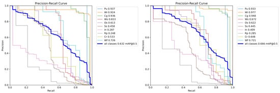
Figure 20. P-R curves of the baseline model and RAC-RTDETR on the GC10-DET dataset.

From the P-R curves of the generalization experiments, it can be seen that RAC-RTDETR achieves an overall MAP improvement of 3.4% over the baseline model, indicating better generalization. Furthermore, RAC-RTDETR shows significant performance improvements in 7 out of 10 defect categories, with the Inclusion (In) class showing the most notable increase of 12.2%. In the remaining three categories with no improvement, the MAP only decreased by 0.1%, 1.3%, and 0.5%, which is acceptable compared to the improvements observed.

We also compared the actual detection results of RAC-RTDETR with those of the baseline model, as shown in Figure 21.

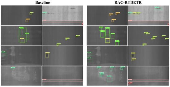
Figure 21. Detection result of the baseline model and RAC-RTDETR on the GC10-DET dataset.

By observing the actual detection results on the GC10-DET dataset, it can be seen that RAC-RTDETR demonstrates superior detection performance for small and edge targets in low-contrast environments. Generalization experiments further show that RAC-RTDETR is capable of adapting to more complex defect detection scenarios.

The comparison of the detection performance of the baseline model and RAC-RTDETR on the Welding defect detection dataset is shown in Figure 22.

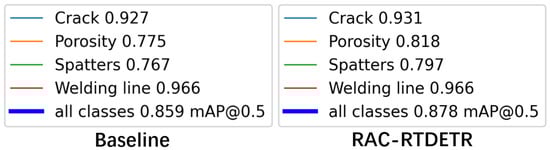
Figure 22. The comparison results of the baseline model and RAC-RTDETR on the Welding defect detection dataset.

As can be seen from Figure 22, compared with the baseline model, the detection accuracy of all defect categories of RAC-RTDETR has been improved, indicating that RAC-RTDETR performs better than the baseline model in the detection of larger targets.

6. Conclusions

To address the challenges of low detection accuracy, large model size, high complexity, and poor real-time performance in steel surface defect detection, we propose RAC-RTDETR, a lightweight and efficient real-time small-object detection algorithm. Based on the RTDETR-R18 model, RAC-RTDETR optimizes the backbone network, AIFI module, and upsampling module to enhance model performance. Extensive experiments on the NEU-DET and GC10-DET datasets validate the effectiveness of these improvements. Comparison results show that RAC-RTDETR achieves a 3.47% increase in detection accuracy, a 36.18% reduction in parameters, a 40.70% decrease in complexity, and a 7.96% increase in detection speed compared to the baseline model, demonstrating a balance of accuracy, lightweight design, and real-time performance. Ablation studies further confirm the model’s improved stability and performance across various steel defect types. Future work will focus on further optimization, particularly for Patches-type defects.

References

- Xu, H.; Zhang, Z.; Ye, H.; Song, J.; Chen, Y. Efficient Steel Surface Defect Detection via a Lightweight YOLO Framework with Task-Specific Knowledge-Guided Optimization. Electronics 2025, 14, 2029. [Google Scholar] [CrossRef]
- Chen, B.; Zha, J.; Cai, Z.; Wu, M. Predictive modelling of surface roughness in precision grinding based on hybrid algorithm. CIRP J. Manuf. Sci. Technol. 2025, 59, 1–17. [Google Scholar] [CrossRef]
- Ge, J.; Yao, Z.; Wu, M.; Almeida, J.H.S., Jr.; Jin, Y.; Sun, D. Tackling data scarcity in machine learning-based CFRP drilling performance prediction through a Broad Learning System with Virtual Sample Generation (BLS-VSG). Compos. Part B Eng. 2025, 305, 112701. [Google Scholar] [CrossRef]
- Wu, M.; Yao, Z.; Ye, L.; Verbeke, M.; Karsmakers, P.; Reynaerts, D. Geometrical Feature Classification in Electrical Discharge Machining Using In-Process Monitoring and Machine Learning. Procedia CIRP 2025, 137, 462–467. [Google Scholar] [CrossRef]
- Redmon, J.; Divvala, S.; Girshick, R.; Farhadi, A. You only look once: Unified, real-time object detection. In Proceedings of the IEEE Conference on Computer Vision and Pattern Recognition, Denver, CO, USA, 3–7 June 2016; pp. 779–788. [Google Scholar]
- Liu, W.; Anguelov, D.; Erhan, D.; Szegedy, C.; Reed, S.; Fu, C.Y.; Berg, A.C. Ssd: Single shot multibox detector. In Proceedings of the European Conference on Computer Vision, Amsterdam, The Netherlands, 11–14 October 2016; Springer: Berlin/Heidelberg, Germany, 2016; pp. 21–37. [Google Scholar]
- Girshick, R. Fast r-cnn. In Proceedings of the IEEE International Conference on Computer Vision, Santiago, Chile, 7–13 December 2015; pp. 1440–1448. [Google Scholar]
- Zhao, Y.; Lv, W.; Xu, S.; Wei, J.; Wang, G.; Dang, Q.; Liu, Y.; Chen, J. Detrs beat yolos on real-time object detection. In Proceedings of the IEEE/CVF Conference on Computer Vision and Pattern Recognition, Seattle, WA, USA, 16–22 June 2024; pp. 16965–16974. [Google Scholar]
- Bao, Y.; Song, K.; Liu, J.; Wang, Y.; Yan, Y.; Yu, H.; Li, X. Triplet-graph reasoning network for few-shot metal generic surface defect segmentation. IEEE Trans. Instrum. Meas. 2021, 70, 5011111. [Google Scholar] [CrossRef]
- Lv, X.; Duan, F.; Jiang, J.j.; Fu, X.; Gan, L. Deep metallic surface defect detection: The new benchmark and detection network. Sensors 2020, 20, 1562. [Google Scholar] [CrossRef] [PubMed]
- Krummenacher, G.; Ong, C.S.; Koller, S.; Kobayashi, S.; Buhmann, J.M. Wheel defect detection with machine learning. IEEE Trans. Intell. Transp. Syst. 2017, 19, 1176–1187. [Google Scholar] [CrossRef]
- Liu, X.; Gao, J. Surface defect detection method of hot rolling strip based on improved SSD model. In Proceedings of the International Conference on Database Systems for Advanced Applications, Taipei, Taiwan, 11–14 April 2021; Springer: Berlin/Heidelberg, Germany, 2021; pp. 209–222. [Google Scholar]
- Liang, C.; Wang, Z.Z.; Liu, X.L.; Zhang, P.; Tian, Z.W.; Qian, R.L. SDD-Net: A Steel Surface Defect Detection Method Based on Contextual Enhancement and Multiscale Feature Fusion. IEEE Access 2024, 12, 185740–185756. [Google Scholar] [CrossRef]
- Lu, S.; Liang, Y.; Ren, Z.; Yu, X.; Wang, X. FEP-YOLO: A lightweight steel surface defect detection method for resource-constrained devices. Meas. Sci. Technol. 2025, 36, 076016. [Google Scholar] [CrossRef]
- Sun, W.; Meng, N.; Chen, L.; Yang, S.; Li, Y.; Tian, S. CTL-YOLO: A Surface Defect Detection Algorithm for Lightweight Hot-Rolled Strip Steel Under Complex Backgrounds. Machines 2025, 13, 301. [Google Scholar] [CrossRef]
- Liao, L.; Song, C.; Wu, S.; Fu, J. A novel YOLOv10-based algorithm for accurate steel surface defect detection. Sensors 2025, 25, 769. [Google Scholar] [CrossRef] [PubMed]
- Leng, Y.; Liu, J. Improved faster R-CNN for steel surface defect detection in industrial quality control. Sci. Rep. 2025, 15, 30093. [Google Scholar] [CrossRef] [PubMed]
- Gao, B.; Zhao, H.; Miao, X. A novel multi-model cascade framework for pipeline defects detection based on machine vision. Measurement 2023, 220, 113374. [Google Scholar] [CrossRef]
- Mao, H.; Gong, Y. Steel surface defect detection based on the lightweight improved RT-DETR algorithm. J. Real-Time Image Process. 2025, 22, 28. [Google Scholar] [CrossRef]
- Su, F.; Meng, P. EL-DETR: A lightweight steel surface defect detection model. Meas. Sci. Technol. 2025, 36, 116003. [Google Scholar] [CrossRef]
- Zhou, S.; Cai, Y.; Zhang, Z.; Yin, J. MESC-DETR: An Improved RT-DETR Algorithm for Steel Surface Defect Detection. Electronics 2025, 14, 2232. [Google Scholar] [CrossRef]
- Vaswani, A.; Shazeer, N.; Parmar, N.; Uszkoreit, J.; Jones, L.; Gomez, A.N.; Kaiser, Ł.; Polosukhin, I. Attention is all you need. In Proceedings of the Advances in Neural Information Processing Systems, Long Beach, CA, USA, 4–9 December 2017; Volume 30. [Google Scholar]
- Wang, C.Y.; Yeh, I.H.; Mark Liao, H.Y. Yolov9: Learning what you want to learn using programmable gradient information. In Proceedings of the European Conference on Computer Vision, Milan, Italy, 29 September–4 October 2024; Springer: Berlin/Heidelberg, Germany, 2024; pp. 1–21. [Google Scholar]
- Cai, X.; Lai, Q.; Wang, Y.; Wang, W.; Sun, Z.; Yao, Y. Poly kernel inception network for remote sensing detection. In Proceedings of the IEEE/CVF Conference on Computer Vision and Pattern Recognition, Seattle, WA, USA, 16–22 June 2024; pp. 27706–27716. [Google Scholar]
- He, K.; Zhang, X.; Ren, S.; Sun, J. Deep residual learning for image recognition. In Proceedings of the IEEE Conference on Computer Vision and Pattern Recognition, Las Vegas, NV, USA, 27–30 June 2016; pp. 770–778. [Google Scholar]
- Hu, J.; Shen, L.; Sun, G. Squeeze-and-excitation networks. In Proceedings of the IEEE Conference on Computer Vision and Pattern Recognition, Salt Lake City, UT, USA, 18–23 June 2018; pp. 7132–7141. [Google Scholar]
- Woo, S.; Park, J.; Lee, J.Y.; Kweon, I.S. Cbam: Convolutional block attention module. In Proceedings of the European Conference on Computer Vision (ECCV), Munich, Germany, 8–14 September 2018; pp. 3–19. [Google Scholar]
- Wang, Q.; Wu, B.; Zhu, P.; Li, P.; Zuo, W.; Hu, Q. ECA-Net: Efficient channel attention for deep convolutional neural networks. In Proceedings of the IEEE/CVF Conference on Computer Vision and Pattern Recognition, Seattle, WA, USA, 13–19 June 2020; pp. 11534–11542. [Google Scholar]
- Wu, M.; Yao, Z.; Verbeke, M.; Karsmakers, P.; Gorissen, B.; Reynaerts, D. Data-driven models with physical interpretability for real-time cavity profile prediction in electrochemical machining processes. Eng. Appl. Artif. Intell. 2025, 160, 111807. [Google Scholar] [CrossRef]
- Liu, W.; Lu, H.; Fu, H.; Cao, Z. Learning to upsample by learning to sample. In Proceedings of the IEEE/CVF International Conference on Computer Vision, Paris, France, 1–6 October 2023; pp. 6027–6037. [Google Scholar]
Disclaimer/Publisher’s Note: The statements, opinions and data contained in all publications are solely those of the individual author(s) and contributor(s) and not of MDPI and/or the editor(s). MDPI and/or the editor(s) disclaim responsibility for any injury to people or property resulting from any ideas, methods, instructions or products referred to in the content. |
© 2025 by the authors. Licensee MDPI, Basel, Switzerland. This article is an open access article distributed under the terms and conditions of the Creative Commons Attribution (CC BY) license (https://creativecommons.org/licenses/by/4.0/).