Multi-Objective Optimal Scheduling of Park-Level Integrated Energy System Based on Trust Region Policy Optimization Algorithm

Abstract

In the context of dual-carbon goals, Park-Level Integrated Energy Systems (PIES) are pivotal for enhancing renewable energy integration and promoting clean, efficient energy use. However, the inherent non-linearity from multi-energy coupling and the high dimensionality of operational data present substantial challenges for conventional scheduling optimization methods. To overcome these obstacles, this paper introduces a novel multi-objective scheduling framework for PIES leveraging deep reinforcement learning. We innovatively formulate the scheduling task as a Markov Decision Process (MDP) and employ the Trust Region Policy Optimization (TRPO) algorithm, which is adept at handling continuous action spaces. The state and action spaces are meticulously designed according to system constraints and user demands. A comprehensive reward function is then established to concurrently pursue three objectives: minimum operating cost, minimum carbon emissions, and maximum exergy efficiency. Through comparative analyses against other AI-based algorithms, our results demonstrate that the proposed method significantly lowers operating costs and carbon footprint while enhancing overall exergy efficiency. This validates the model’s effectiveness and superiority in addressing the complex multi-objective scheduling challenges inherent in modern energy systems.

1. Introduction

Amid the global imperative to address climate change, a paradigm shift towards modern energy systems that are secure, reliable, low-carbon, and efficient has become a universal objective [1]. Park-level Integrated Energy Systems (PIES) present a forward-thinking solution for constructing future energy infrastructures by physically integrating multiple energy vectors and synergistically optimizing all segments of the source-network-load-storage chain [2]. The core principle of a PIES is to maximize energy efficiency and enhance the integration of renewable energy sources through multi-energy complementarity and cascaded utilization [3]. However, due to the fact that PIES typically aggregates multiple types of equipment or energy sources internally, endowing it with strong coupling characteristics and uncertainty, this poses challenges for the optimization control of PIES.

To date, approaches to addressing multi-energy coupling characteristics in complex PIESs have primarily relied on decoupling, phased, or hierarchical optimization scheduling. Literature [4] established a synergistic optimization framework for multi-energy flows of electricity, heat, and hydrogen. Literature [5] developed a two-stage optimization model based on predictive modeling. Literature [6] formulates an objective function for maximizing total profit and employs a hierarchical algorithm for its solution. Furthermore, if the aforementioned methods aim to incorporate uncertainties associated with renewable energy sources or loads, techniques such as stochastic programming or robust optimization must be employed. Literature [7] employs the Monte Carlo method to address uncertainties in load and wind power. Literature [8] proposes a robust optimization model for analyzing the interdependencies among natural gas, coal, and power infrastructure, which simultaneously accounts for operational constraints and wind energy uncertainty. Literature [9] proposes a distributed robust daily advance scheduling model to incorporate uncertainties in ambient temperature, solar radiation, and residential electricity load. Although the above methods have promoted the development of PIES to a certain extent, these model-based optimization approaches often face the dilemma of balancing modeling accuracy and computational efficiency when dealing with non-linear systems [10,11].

On the other hand, as the penetration rate of distributed renewable energy increases, the role of PIES in the electricity market is also growing steadily [12]. Literature [13] proposes a bidding model based on a master-slave game between energy suppliers and the energy market to maximize the profit of the PIES system. Literature [14] proposes a two-stage framework for enabling IES participation in electricity markets. Literature [15] proposes an operational cost optimization method for regional integrated energy systems under uncertain power market conditions. These studies all take economic optimization as their starting point. However, focusing solely on economic indicators may lead to situations where energy efficiency is not effectively utilized, while also hindering environmental protection. Based on this consideration, the literature [16] conducted a multi-objective optimization that incorporated both minimizing operational costs and minimizing carbon emissions. Literature [17] proposes an optimization objective for PIES that minimizes both daily total operating costs and wind power curtailment. Literature [18] constructed a multi-objective optimization model that calculates annual total costs, external power ratios, and carbon emission values to achieve optimal overall performance in economic, autonomy, and environmental aspects. It is evident that considering multiple objectives simultaneously has become a prevailing trend in the optimization of PIES. While these approaches offer novel perspectives for future developments in PIES optimization control, some still rely on precise system modeling. Others, though based on model-free control methods utilizing spatial exploration, fail to meet system requirements in terms of computational efficiency. Therefore, employing an optimization method capable of addressing system nonlinearity and reducing dependence on models is particularly crucial.

To date, reinforcement learning has garnered significant attention from researchers as a data-driven, model-free control approach [19,20]. Its key advantage lies in its ability to learn sufficiently complex patterns to represent the impact of randomness without requiring strong assumptions or precise modeling of specific distributions (e.g., Gaussian, Poisson) [21]. As long as randomness is reflected in the training data, deep neural networks can approximate functions to learn these patterns and identify corresponding optimal strategies [22]. This model-free nature inherently adapts to source load uncertainty and avoids the need for explicit system mathematical models, distinguishing it from the methods mentioned in [23]. Furthermore, PIES dynamic scheduling is fundamentally a stochastic sequential decision problem, aligning closely with the theoretical framework of reinforcement learning (RL). Therefore, applying RL to the PIES domain is a natural and advanced development [24]. For example, the study [25] applied reinforcement learning to integrated nuclear-renewable energy systems, achieving unified dispatch of renewable energy, hydrogen, and energy storage systems. Study [26] employed the Soft Actor-Critic (SAC) algorithm for optimal scheduling of a combined energy storage system integrating electricity, thermal energy, and hydrogen storage. Study [27] integrates Carbon Capture and Storage (CCS) technology with Gas-To-Power (G2P) conversion equipment within a combined gas-to-power system. It employs a dual-delay deep deterministic policy gradient algorithm to achieve real-time scheduling decisions that simultaneously minimize both operational costs and carbon emissions. Similarly, study [28] sets economic optimization and minimal carbon emissions as dispatch objectives, achieving optimization through the Deep Deterministic Policy Gradient (DDPG) algorithm. Similarly, other works include literature [29,30,31] and so on.

Although significant progress has been made in applying RL to the PIES system, there is still room for improvement. For example, in the aforementioned study, carbon emissions were merely treated as constraints or viewed as detrimental factors. The potential utilization of carbon dioxide as a resource was not considered, which to some extent limited the overall benefits of PIES. However, utilizing CCS and Power-to-Gas (P2G) technology while incorporating carbon market price transactions can more effectively enhance the system’s renewable energy absorption capacity, reduce operational costs, and lower carbon emissions [32,33,34]. Therefore, under the RL mechanism, integrating CCS and P2G while incorporating carbon trading is crucial for addressing gaps in existing research. Equally important, existing studies on carbon trading based on non-RL mechanisms struggle to adapt to dynamic market conditions and lack scientifically grounded pricing adjustment mechanisms. This will prevent the full realization of emission reduction potential.

Therefore, this paper undertakes the following research:

• To address the challenges of insufficient adaptability and excessive reliance on model accuracy faced by model-based optimization methods in dynamic scheduling scenarios, this paper proposes a PIES low-carbon economic optimization scheduling scheme based on the Trust Region Policy Optimization algorithm (TRPO).
• To address the incentive deficiency inherent in traditional single-price carbon pricing mechanisms, this paper proposes a market-feedback-based carbon trading model featuring dynamic parameter optimization. This model integrates a Ladder-style carbon trading with carbon emission reduction equipment. This process also takes into account the role of waste heat recovery.
• To align with the PIES system’s primary feature of multi-energy integration, this paper introduces the concept of Exergy to evaluate the efficiency of energy conversion within the system. Subsequently, an optimization framework is constructed using the Approximate Ideal Solution Ranking method, prioritizing the lowest system operating costs, minimal carbon emissions, and maximum Exergy efficiency.

2. Integrated Energy Systems at the Campus Level

2.1. A Multi-Objective Optimal Scheduling Model for Park-Level Integrated Energy Systems

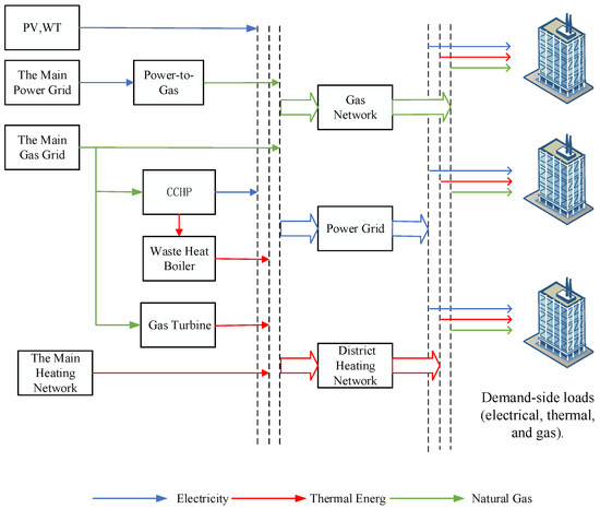
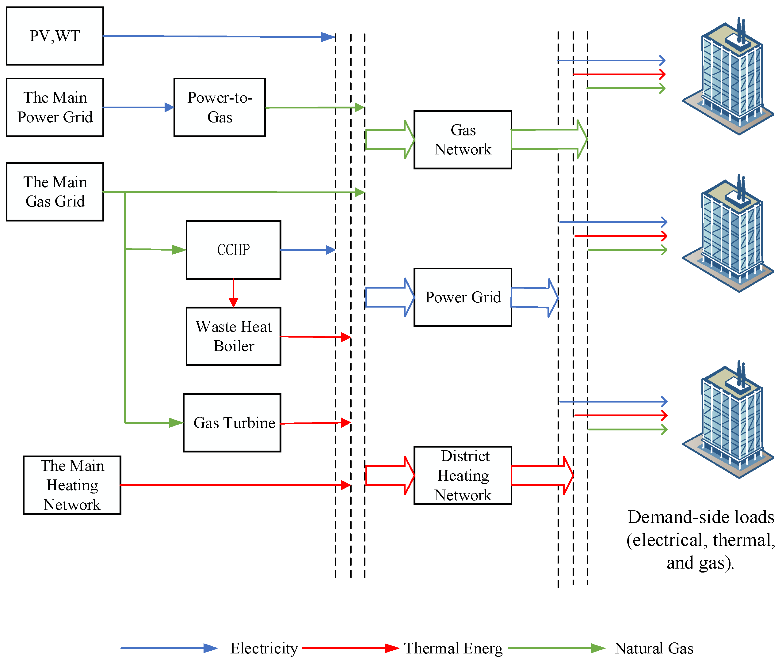
The multi-objective optimal scheduling model of the park-level integrated energy system constructed in this paper is shown in Figure 1, and the system achieves the complementary advantages of different energy sources and improves the efficiency of energy utilization by coupling a variety of energy conversion equipment.

Figure 1. Overall structure of the PIES system.

On the energy supply side, the cogeneration units, consisting of Gas Turbines (GT) and waste heat boilers (WHB), convert natural gas to electricity and heat, the gas boilers (GB) convert natural gas to heat, and the power-to-gas unit converts CO₂ generated by the park’s IESs into natural gas for use by the CHP units and the gas boiler units; the PIES is supplied with energy from the external grid, the external gas grid, and the wind turbines.

2.2. Modeling of Cogeneration Units

The cogeneration unit consists of two parts: a gas turbine and a waste heat boiler.

2.2.1. Gas Turbine Models

Gas turbines (GT) have the advantages of low operating cost, fast start-up, safety and reliability, and good load-following, etc. Although the output power of a single unit is not high, the cogeneration unit formed around it and the waste heat boiler has a higher energy utilization rate than that of a large unit, and is widely used in IESs. GT is a typical non-linear equipment, its power generation efficiency is greatly affected by the unit out-put, this paper adopts the third-order model to describe the relationship between its gas-to-electricity efficiency and the output electric power, the equipment model is:

$$\left\{\begin{array}{l}{P}_{\mathrm{GT}}\left(t\right)={\eta }_{\mathrm{GT}}^e{G}_{\mathrm{GT}}\left(t\right)\\ H_{\mathrm{GT}}\left(t\right)={\eta }_{\mathrm{GT}}^h{G}_{\mathrm{GT}}\left(t\right)\\ C_{\mathrm{GT}}(t)={\chi }_h\left(\gamma P_{\mathrm{GT}}\left(t\right)+H_{\mathrm{GT}}\left(t\right)\right)\end{array}\right.$$

(1)

where $G_{\mathrm{GT}}\left(t\right)$, $P_{\mathrm{GT}}\left(t\right)$, $H_{\mathrm{GT}}\left(t\right)$ represent the input natural gas power, electric power output, and thermal power output of the GT at time period $t$, respectively; ${\eta }_{\mathrm{GT}}^{\mathrm{e}}(t)$, ${\eta }_{\mathrm{GT}}^h(t)$ represent the gas-to-electricity efficiency and gas-to-thermal efficiency of the GT at time period $t$, respectively; $C_{\mathrm{GT}}(t)$ denotes the CO₂ emissions of the GT at time period $t$.

2.2.2. Waste Heat Boiler Model

Waste Heat Boilers (WHB) can collect the high-temperature flue gases from GTs and provide heat to users, greatly improving the utilization of the heat released from the combustion of natural gas. Waste heat utilization is modeled as:

$$\left\{\begin{array}{l}{H}_{\mathrm{WHB}\mathrm{out}}\left(t\right)={\eta }_{\mathrm{WHB}}{H}_{\mathrm{WHBin}}\left(t\right)\\ H_{\mathrm{WHB}\mathrm{in}}\left(t\right)=H_{\mathrm{GT}}\left(t\right)\end{array}\right.$$

(2)

where $H_{\mathrm{WHBin}}\left(t\right)$, $H_{\mathrm{WHBout}}\left(t\right)$ present the input and output thermal power of the WHB during time period $t$, respectively; ${\eta }_{\mathrm{WHB}}$ denotes the heat loss rate of the WHB.

2.3. Power-to-Gas Unit Modeling

The operation of Power-to-Gas (P2G) systems can be divided into two stages: hydrogen production via water electrolysis and methane synthesis from hydrogen.

$$\left\{\begin{array}{l}\Delta \mathrm{H}=-165.0 \mathrm{kj}{·\mathrm{mol}}^{-1}\\ {\mathrm{H}}_2\mathrm{O}\stackrel{Energize}{\to }{\mathrm{H}}_2+{\displaystyle \frac{1}{2}}{\mathrm{O}}_2\\ {4\mathrm{H}}_2{+\mathrm{CO}}_2\stackrel{Catalyst}{\to }{\mathrm{CH}}_4{+2\mathrm{H}}_2\mathrm{O}\end{array}\right.$$

(3)

where $\Delta \mathrm{H}$ denotes the entropy of the chemical reaction. A negative entropy value indicates that the reaction is exothermic, releasing heat to the surroundings.

In the process of hydrogen methanation, the reaction heat is typically released into the air, which not only causes environmental pollution but also leads to energy waste. This study considers recovering the waste heat generated during the synthetic natural gas (SNG) production by P2G systems and utilizing it for heat supply to the demand side. This approach not only improves energy efficiency but also reduces environmental pollution. The rate of hydrogen methanation and the corresponding heat released during the reaction per unit time are calculated using Equation (4):

$$\left\{\begin{array}{l}{V}_{{\mathrm{CH}}_4}={\displaystyle \frac{(P_{\mathrm{P}2\mathrm{G}}/V_{{\mathrm{H}}_2})·{\rho }_{{\mathrm{H}}_2}·(Q_{{\mathrm{CH}}_4}/{\rho }_{{\mathrm{CH}}_4})M_{{\mathrm{CH}}_4}}{1.44\times {10}^7·M_{{\mathrm{H}}_2}}}\\ H_{{\mathrm{CH}}_4}={\displaystyle \frac{(P_{\mathrm{P}2\mathrm{G}}/V_{{\mathrm{H}}_2})·{\rho }_{{\mathrm{H}}_2}·Q_{\mathrm{P}2\mathrm{G}}}{1.44\times {10}^4·M_{{\mathrm{H}}_2}}}·\vartheta \end{array}\right.$$

(4)

where $V_{{\mathrm{H}}_2}$, $V_{{\mathrm{CH}}_4}$ represent the hydrogen production rate via water electrolysis and the hydrogen methanation rate, respectively; $M_{{\mathrm{H}}_2}$, $M_{{\mathrm{CH}}_4}$ denote the molar masses of hydrogen and methane, respectively; ${\rho }_{{\mathrm{H}}_2}$, ${\rho }_{{\mathrm{CH}}_4}$ refer to the densities of hydrogen and methane, respectively; $Q_{{\mathrm{CH}}_4}$, $Q_{\mathrm{P}2\mathrm{G}}$ represent the calorific value of methane and the amount of heat released during methane synthesis in the P2G process, respectively; $P_{\mathrm{P}2\mathrm{G}}$ denotes the electrical energy consumed in the P2G process; $\vartheta$ refers to the proportion of reaction heat that can be recovered. Calculations show that for every $1 \mathrm{kW}·\mathrm{h}$ units of electricity consumed, the P2G system generates $0.12 \mathrm{kW}·\mathrm{h}$ units of recoverable heat.

This study considers recovering the waste heat generated during synthetic natural gas (SNG) production in P2G systems and utilizing it for heat supply on the demand side, thereby improving energy efficiency and reducing environmental pollution. The P2G system model with waste heat recovery is described as follows:

$$\left\{\begin{array}{l}{G}_{\mathrm{P}2\mathrm{G}}(t)={\eta }_{\mathrm{P}2\mathrm{G},g}{P}_{\mathrm{P}2\mathrm{G}}(t)\\ H_{\mathrm{P}2\mathrm{G}}(t)={\eta }_{\mathrm{P}2\mathrm{G},h}{P}_{\mathrm{P}2\mathrm{G}}(t)\\ C_{\mathrm{P}2\mathrm{G}}(t)={\eta }_{\mathrm{P}2\mathrm{G},c}{G}_{\mathrm{P}2\mathrm{G}}(t)\\ C_{\mathrm{P}2\mathrm{G}}(t)<C_{\mathrm{GT}}(t)+C_{\mathrm{GB}}(t)\end{array}\right.$$

(5)

where $G_{\mathrm{P}2\mathrm{G}}(t)$, $H_{\mathrm{P}2\mathrm{G}}(t)$ represent the amount of synthetic natural gas produced and the amount of waste heat recovered by the P2G system during time period $t$, respectively; $P_{\mathrm{P}2\mathrm{G}}(t)$ denotes the electricity consumption of the P2G system during time period t; ${\eta }_{\mathrm{P}2\mathrm{G},\mathrm{g}}$, ${\eta }_{\mathrm{P}2\mathrm{G},\mathrm{h}}$ and ${\eta }_{\mathrm{P}2\mathrm{G},\mathrm{c}}$ represent the operational efficiency of the P2G system, the waste heat recovery efficiency, and the amount of CO₂ consumed per unit of synthetic natural gas produced, respectively; $C_{\mathrm{P}2\mathrm{G}}$ denotes the total amount of CO₂ consumed by the power-to-gas (P2G) system. Note: In this paper, to focus on system-level collaborative optimization analysis and ensure model manageability, the gas production efficiency and waste heat recovery efficiency of the P2G system are modeled as constants. When conducting equipment-level analysis or addressing uncertainties, the dynamic variation in efficiency with factors such as equipment load rate and operating temperature should be considered.

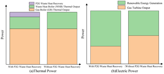
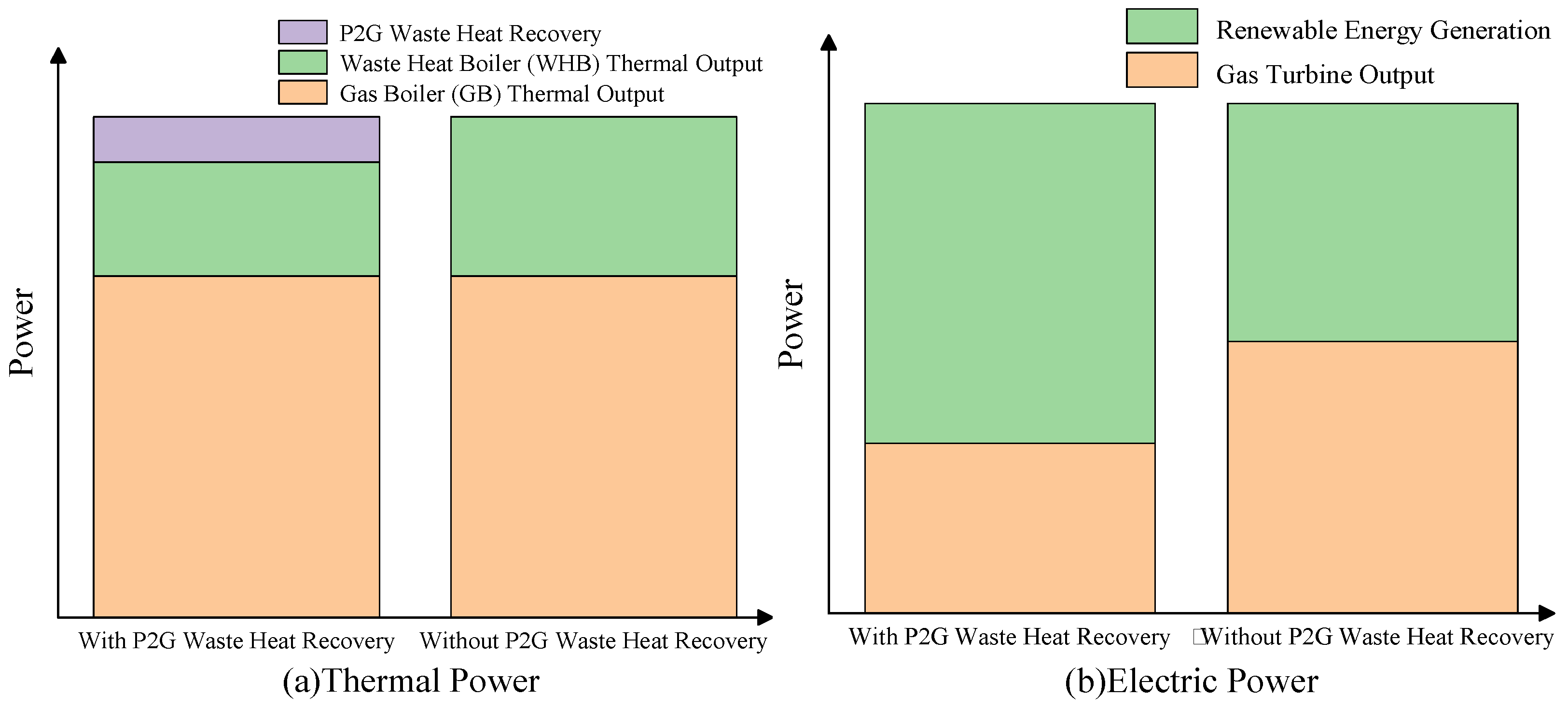
The mechanism by which recovered P2G waste heat promotes the consumption of renewable electricity is illustrated in Figure 2.

Figure 2. The mechanism by which P2G waste heat recovery enhances renewable energy integration.

As shown in Figure 2, when renewable energy output is abundant, the thermal output of the GT is reduced due to the recovery of P2G waste heat. This leads to a corresponding decrease in the GT’s power generation, thereby creating additional capacity for wind power integration.

2.4. Gas Boiler Model

In the thermal energy supply section of the PIES, the gas boiler serves as a key heating device. Its typical structure comprises five functional modules: a fuel control valve, a combustion system, an intelligent control unit, a temperature sensing device, and a heat exchange chamber.

$$\left\{\begin{array}{l}{H}_{\mathrm{GB}}\left(t\right)={\eta }_{\mathrm{GB}}{G}_{\mathrm{GB}}\left(t\right)\\ C_{\mathrm{GB}}\left(t\right)={\chi }_h{H}_{\mathrm{GB}}\left(t\right)\end{array}\right.$$

(6)

where ${\eta }_{\mathrm{GB}}$ represents the efficiency of the gas boiler in converting natural gas into thermal energy. $G_{\mathrm{GB}}\left(t\right)$ represents the amount of natural gas input into the gas boiler during time period $t$. $C_{\mathrm{GB}}\left(t\right)$ represents the amount of carbon dioxide emitted by the gas boiler during time period $t$.

2.5. Energy Hub Model

In addition to the operational constraints of each unit, the system must also satisfy power balance constraints.

$$\begin{array}{l}{H}_{\mathrm{CHP}}+H_{\mathrm{GB}}+H_{\mathrm{P}2\mathrm{G}}=H_{\mathrm{load}}\\ E_{\mathrm{grid}}+P_{\mathrm{CHP}}+P_{\mathrm{WT}}=E_{\mathrm{load}}+P_{\mathrm{P}2\mathrm{G}}\\ G_{\mathrm{gas}}+G_{\mathrm{P}2\mathrm{G}}=F_{\mathrm{GB}}+G_{\mathrm{GT}}+G_{\mathrm{load}}\end{array}$$

(7)

The above equations represent the thermal power balance, electrical power balance constraint, and natural gas balance constraint of the system, respectively.

2.6. Carbon Capture System

The PIES carbon emission sources constructed in this study primarily encompass four components: electricity procurement from external grids, gas consumption by end-users, gas turbine operations, and gas boiler operations. This paper attributes carbon emissions from externally procured electricity to upstream thermal power plants, excluding them from the total emissions of this system. Carbon dioxide emissions from distributed natural gas usage within the system exhibit characteristics such as dispersed emission points and temporal uncertainty. Addressing this feature, the carbon capture system designed in this model specifically treats CO₂ from centralized emission sources within the industrial park. The treated carbon resources have two utilization pathways: a portion is transported to methanation units as synthesis feedstock, while the remainder is compressed, stored, and entered into the carbon trading market to generate revenue. The formula is as follows:

$$\left\{\begin{array}{l}{P}_{\mathrm{CCS}}(t)=\alpha C_{\mathrm{CCS}}(t)\hfill \\ f_T(t)=\omega C_{\mathrm{CCS}}(t)\hfill \end{array}\right.$$

(8)

where $\omega$ is the price coefficient for selling one unit mass of CO₂. $\alpha$ is the power consumption coefficient of the equipment. $C_{\mathrm{CCS}}(t)$ represents the amount of CO₂ captured by the equipment at time $t$; $P_{\mathrm{CCS}}(t)$ represents the power consumption of the carbon capture equipment at time $t$; $f_T(t)$ represents the profit generated from selling carbon dioxide at time $t$.

2.7. Wind Power

In addition to the operational constraints of each unit, the system must also satisfy power balance constraints.

$$P_{\mathrm{WT}}(t)=\left\{\begin{array}{ll}0\hfill & v\le v_{\mathrm{in} }\hfill \\ P_{\mathrm{WT},c}{\displaystyle \frac{v^3-v_{\mathrm{in} }^3}{v_c^3-v_{\mathrm{in} }^3}}\hfill & v_{\mathrm{in} }\le v\le v_c\hfill \\ P_{\mathrm{WT},c}\hfill & v_c\le v\le v_{\mathrm{out} }\hfill \\ 0\hfill & v\ge v_{\mathrm{out} }\hfill \end{array}\right.$$

(9)

where $v ,v_{\mathrm{in} },v_{\mathrm{c}} ,v_{\mathrm{out} }$ represent the actual wind speed, cut-in wind speed, rated wind speed, and cut-out wind speed of the wind turbine, respectively. $P_{\mathrm{WT},c}$ is the rated electrical power output of the wind turbine generator. $P_{\mathrm{WT}}(t)$ represents the electrical power output of the wind turbine at time $t$.

3. Multi-Objective Optimal Scheduling Model Considering Exergy Efficiency

This study aims to achieve high-quality and economically efficient energy utilization in the integrated energy system while taking carbon emission targets into account. Accordingly, a multi-objective optimal scheduling model is developed, which simultaneously minimizes system operating cost and carbon emissions, and maximizes exergy efficiency.

3.1. Ladder-Style Carbon Trading for CCS

The carbon emission allowance model is shown in the following equation:

$$\left\{\begin{array}{l}{C}_{\mathrm{PIES}}^{*}=C_{\mathrm{buy}}^{*}+C_{\mathrm{GT}}^{*}+C_{\mathrm{GB}}^{*}+C_{\mathrm{g},\mathrm{LOAD}}^{*}\hfill \\ C_{\mathrm{buy}}^{*}={\chi }_{\mathrm{e}}^{*}{\displaystyle \sum _{t=1}^T{P}_{\mathrm{s}}}(t)\hfill \\ C_{\mathrm{GT}}^{*}={\chi }_{\mathrm{h}}^{*}{\displaystyle \sum _{t=1}^T{C}_{\mathrm{GT}}}(t)\hfill \\ C_{\mathrm{GB}}^{*}={\chi }_{\mathrm{h}}^{*}{\displaystyle \sum _{t=1}^T{C}_{\mathrm{GB}}}(t)\hfill \\ C_{\mathrm{g},\mathrm{LOAD}}^{*}={\chi }_{\mathrm{g}}^{*}{\displaystyle \sum _{t=1}^T{G}_{\mathrm{LOAD}}}(t)\hfill \end{array}\right.$$

(10)

where $C_{\mathrm{PIES}}^{*},C_{\mathrm{buy}}^{*},C_{\mathrm{GT}}^{*},C_{\mathrm{GB}}^{*},C_{\mathrm{g},\mathrm{LOAD}}^{*}$ represent the carbon emission allowances obtained by PIES, respectively, and the carbon emission allowances obtained by each piece of equipment during PIES operation; ${\chi }_{\mathrm{e}}^{*},{\chi }_{\mathrm{h}}^{*},{\chi }_{\mathrm{g}}^{*}$ represent the carbon emission allowance coefficient factors obtained per unit of natural gas consumed by coal-fired units, natural gas-fired units, and end-users, respectively.

The actual carbon emissions model is as follows:

$$\left\{\begin{array}{l}{C}_{\mathrm{PIES}}=C_{\mathrm{buy}}+C_{\mathrm{GT}}+C_{\mathrm{GB}}+C_{\mathrm{g},\mathrm{LOAD}}-C_{\mathrm{CCS}}-C_{\mathrm{P}2\mathrm{G}}\hfill \\ C_{\mathrm{buy}}={\chi }_{\mathrm{e}}{\displaystyle \sum _{t=1}^T{P}_{\mathrm{s}}}(t)\hfill \\ C_{\mathrm{GT}}={\displaystyle \sum _{t=1}^T{C}_{\mathrm{GT}}}(t)\hfill \\ C_{\mathrm{GB}}={\displaystyle \sum _{t=1}^T{C}_{\mathrm{GB}}}(t)\hfill \\ C_{\mathrm{g},\mathrm{LOAD}}={\chi }_{\mathrm{g}}{\displaystyle \sum _{t=1}^T{G}_{\mathrm{LOAD}}}(t)\hfill \\ C_{\mathrm{CCS}}={\displaystyle \sum _{t=1}^T{C}_{\mathrm{CCS}}}(t)\hfill \\ C_{\mathrm{P}2\mathrm{G}}(t)={\eta }_{\mathrm{P}2\mathrm{G},c}{G}_{\mathrm{P}2\mathrm{G}}(t)\hfill \end{array}\right.$$

(11)

where ${\chi }_{\mathrm{e}}$ is the actual carbon emission factor for coal-fired power plants; $C_{\mathrm{PIES}},C_{\mathrm{buy}},C_{\mathrm{GT}},C_{\mathrm{GB}},C_{\mathrm{g},\mathrm{LOAD}},C_{\mathrm{CCS}},C_{\mathrm{P}2\mathrm{G}}(t)$ represent the actual carbon emissions of PIES, the actual carbon emissions of each piece of equipment within PIES, the amount of CO₂ consumed by the carbon capture equipment, and the amount of CO₂ consumed by the P2G equipment, respectively; ${\chi }_{\mathrm{g}}$ represents the actual carbon emission coefficient generated per unit of natural gas consumed by users. Therefore, the quantity of carbon emission allowances purchased can be expressed as:

$${C_{\mathrm{PIES}}}^{\prime }=C_{\mathrm{PIES} }-C_{\mathrm{PIES} }^{*}$$

(12)

where ${C_{\mathrm{PIES}}}^{\prime }$ represents the carbon emission allowances that PIES needs to purchase:

$$F_{{\mathrm{CO}}_2}=\left\{\begin{array}{l}\cdots \hfill \\ \psi (1+3\mu )\left({C_{\mathrm{PIES}}}^{\prime }+3l\right)-\psi (3+3\mu )l,\hspace{0.33em}\hspace{0.33em}\hspace{0.33em} -4l\le {C_{\mathrm{PIES}}}^{\prime }\le -3l\hfill \\ \psi (1+2\mu )\left({C_{\mathrm{PIES}}}^{\prime }+2l\right)-\psi (2+\mu )l,\hspace{0.33em}\hspace{0.33em}\hspace{0.33em} -3l\le {C_{\mathrm{PIES}}}^{\prime }\le -2l\hfill \\ \psi (1+\mu )\left({C_{\mathrm{PIES}}}^{\prime }+l\right)-\psi l,\hspace{0.33em}\hspace{0.33em}\hspace{0.33em} -2l\le {C_{\mathrm{PIES}}}^{\prime }\le -l\hfill \\ \psi {C_{\mathrm{PIES}}}^{\prime },\hspace{0.33em}\hspace{0.33em}\hspace{0.33em} -l\le {C_{\mathrm{PIES}}}^{\prime }\le l\hfill \\ \psi (1+\mu )\left({C_{\mathrm{PIES}}}^{\prime }-l\right)+\psi l,\hspace{0.33em}\hspace{0.33em}\hspace{0.33em} l\le {C_{\mathrm{PIES}}}^{\prime }\le 2l\hfill \\ \psi (1+2\mu )\left({C_{\mathrm{PIES}}}^{\prime }-2l\right)+\psi (2+\mu )l,\hspace{0.33em}\hspace{0.33em}\hspace{0.33em} 2l\le {C_{\mathrm{PIES}}}^{\prime }\le 3l\hfill \\ \psi (1+3\mu )\left({C_{\mathrm{PIES}}}^{\prime }-3l\right)+\psi (3+3\mu )l,\hspace{0.33em}\hspace{0.33em}\hspace{0.33em} 3l\le {C_{\mathrm{PIES}}}^{\prime }\le 4l\hfill \\ \cdots \hfill \end{array}\right.$$

(13)

where $l$ represents the length of the carbon emission range for the tiered carbon trading mechanism; $\psi$ denotes the base price for carbon trading; $\mu$ indicates the price growth rate; $F_{{\mathrm{CO}}_2}$ signifies the cost of the tiered carbon trading system.

3.2. Low-Carbon Economy Optimization Dispatch Model

The objective function is:

$$\min F_{\mathrm{PIES},\mathrm{E}}=F_{\mathrm{buy}}$$

(14)

$$\max F_{\mathrm{PIES},\mathrm{C}}=F_{{\mathrm{CO}}_2}-F_{\mathrm{T}}$$

(15)

$$F_{\mathrm{buy} }={\displaystyle \sum _{t=1}^T{c}_{\mathrm{fs}}}(t)P_{\mathrm{buy} }(t)+{\displaystyle \sum _{t=1}^T{c}_{\mathrm{b}}^{\mathrm{g}}}(t)G_{\mathrm{buy} }(t)$$

(16)

$$F_{\mathrm{T}}={\displaystyle \sum _{t=1}^T{f}_{\mathrm{T}}}(t)$$

(17)

where Equation (14) represents the economic objective; Equation (15) represents the carbon emission target; $F_{\mathrm{buy}}$ represents the purchasing cost of PIES; $F_{\mathrm{T}}$ represents the profit obtained from the sale of carbon dioxide; $P_{\mathrm{buy} }(t)$ represents the electricity purchased at time $t$; $G_{\mathrm{buy} }(t)$ represents the natural gas purchased at time $t$; $c_{\mathrm{fs}}(t)$ and $c_{\mathrm{b}}^{\mathrm{g}}(t)$ $c_{\mathrm{b}}^{\mathrm{g}}(t)$ represent the time-of-use electricity price and natural gas price, respectively.

3.3. Exergy Efficiency of the Multi-Energy System

Exergy refers to the portion of energy that can be theoretically converted into mechanical work under given environmental conditions. It is also known as available energy or useful energy. In contrast, the unconvertible part of energy is known as anergy, also referred to as unavailable or non-useful energy. Therefore, any form of energy can be considered as comprising two components: exergy and anergy, i.e.,

$$E=E_x+A_n$$

(18)

where $E$, $E_x$ and $A_n$ represent energy, exergy, and anergy, respectively.

Multi-energy integration has become a mainstream trend in the development of energy systems. The deep coupling and mutual complementarity among heterogeneous energy carriers—such as electricity, gas, hydrogen, heat, carbon-based fuels, and renewable energy—offer greater flexibility and optimization potential for improving the quality and efficiency of energy utilization.

Traditional energy systems based on separated production and specialization typically involve only a single form of energy. Taking the power system as an example, since electricity is the sole energy carrier, its energy efficiency has long been evaluated using conventional energy efficiency metrics, which are defined as the numerical ratio of output energy to input energy:

$${\eta }_{\mathrm{e}}={\displaystyle \frac{E_{\mathrm{out}}}{E_{\mathrm{in}}}}$$

(19)

where ${\eta }_{\mathrm{e}}$ represents the energy efficiency; $E_{\mathrm{in}}$ and $E_{\mathrm{out}}$ denote the input and output energy, respectively.

It is evident that conventional energy efficiency metrics are no longer suitable for multi-energy systems. For example, converting 1 kWh of electricity into 1 kWh of thermal energy in an enclosed space via resistance heating, may appear to have an energy efficiency of 100% in numerical terms, but the process is inherently irreversible, as the thermal energy in the space cannot be recovered and converted back into electricity. This indicates that although the quantity of energy remains unchanged before and after conversion, its quality degrades in the process. Introducing the concept of exergy provides a means to address this issue. The key to evaluating the efficiency of an energy conversion process lies in how much exergy is lost. Therefore, the exergy efficiency of an energy conversion process can be defined as:

$${\eta }_{ex}={\displaystyle \frac{E_{x,out}}{E_{x,in}}}$$

(20)

where ${\eta }_{ex}$ represents the exergy efficiency; $E_{\mathrm{x},\mathrm{in}}$, $E_{\mathrm{x},\mathrm{out}}$ denote the input and output exergy, respectively.

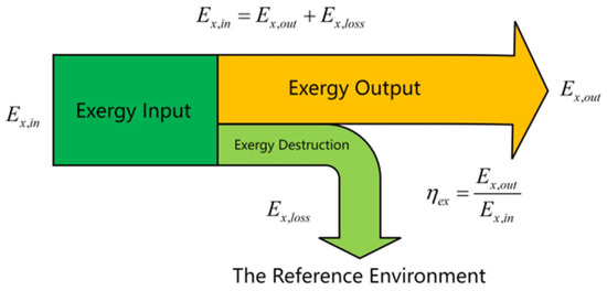
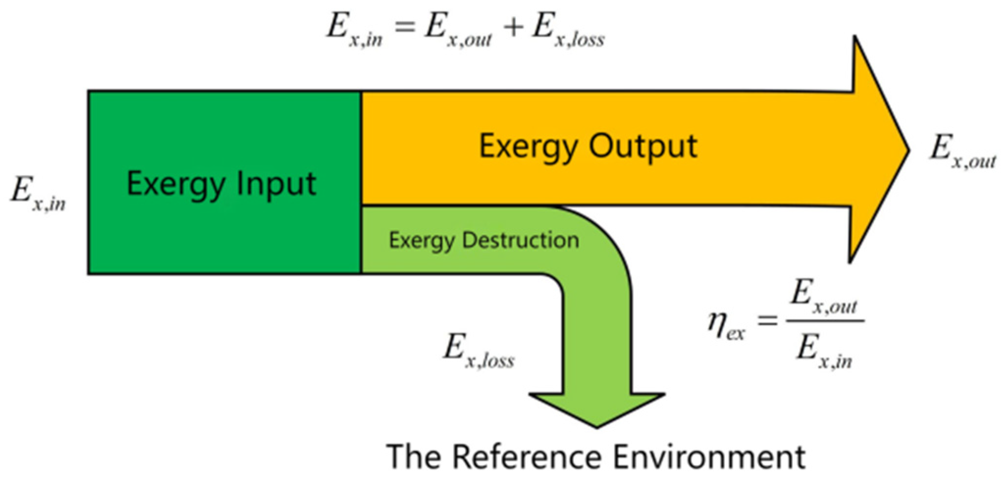
Exergy analysis methods are generally classified into two approaches: black-box models and white-box models. The black-box model treats the system as a closed unit enclosed by opaque boundaries, where exergy efficiency is calculated solely based on external inputs and outputs. In contrast, the white-box model conducts a detailed exergy analysis by dissecting each internal energy conversion process, allowing for the quantification of exergy dissipation at each stage. For an Inte-grated Energy System (IES) involving numerous and diverse energy conversion processes, analyzing each process individually is impractical. Therefore, the black-box model is more suitable for evaluating the overall exergy efficiency of an IES, as illustrated in Figure 3.

Figure 3. Black-box model for IES exergy analysis.

The supply side delivers quantity $E_{\mathrm{x},\mathrm{in}}$ as the input payment to the Integrated Energy System (IES), which then undergoes a series of internal processes such as transmission, conversion, storage, and distribution, ultimately outputting quantity $E_{\mathrm{x},\mathrm{out}}$ as the revenue, in order to meet the diverse energy demands of users within the region.

As previously stated, energy is the sum of exergy and anergy. Assuming that the proportion of exergy in the total energy is denoted by $\lambda$, this ratio varies depending on the quality of the energy. High-quality energy has a higher value of $\lambda$, whereas lower-quality energy corresponds to a lower value of $\lambda$. Mechanical energy is considered the highest-quality form of energy. However, it faces significant challenges in terms of transmission and storage, making its application in Integrated Energy Systems (IES) relatively limited. As a substitute, electricity—being easier to transmit and utilize—is widely adopted. In general, electricity is regarded as having an energy quality comparable to that of mechanical energy, that is:

$${\lambda }_e={\lambda }_m=1$$

(21)

Under typical conditions, the quality factor of gaseous fuel is taken as ${\lambda }_q=0.95$, while the quality factor of thermal energy is given by:

$${\lambda }_h=1-{\displaystyle \frac{T_0}{T_h}}$$

(22)

where $T_0$ and $T_h$ represent the ambient temperature and the temperature of the thermal load, respectively.

Therefore, the objective of maximizing exergy efficiency is formulated as follows:

$$\max S={\displaystyle \sum _{t=1}^T\frac{{\lambda }_e{L}_e^t+{\lambda }_h{L}_h^t+{\lambda }_q{L}_q^t}{P_{\mathrm{grid}}^t+Q_{\mathrm{gas}}^t+P_{\mathrm{wt}}^t+P_{\mathrm{pv}}^t}}$$

(23)

3.4. The Constraints Are as Follows:

Equation (24) represents the electrical power balance constraint, where $P_{\mathrm{pv} }(t)$ denotes the output of new energy sources; Equation (25) represents the thermal power balance constraint; Equation (26) represents the gas power balance constraint; Equation (27) represents the purchased energy constraint, where $P_{\mathrm{buy} }^{\max }$ and $G_{\mathrm{buy} }^{\max }$ denote the upper limits for purchased electricity power and purchased gas power, respectively; Equation (28) represents the electrolyzer operation constraint, where $P_{\mathrm{P}2\mathrm{G}}^{\min }$ and $P_{\mathrm{P}2\mathrm{G}}^{\max }$ denote the lower and upper limits of electrolyzer input electrical power, respectively, and $\Delta P_{\mathrm{P}2\mathrm{G}}^{\min }$ and $\Delta P_{\mathrm{P}2\mathrm{G}}^{\max }$ denote the lower and upper limits of electrolyzer ramping rates, respectively; Equation (29) represents the gas turbine operation constraint, where $G_{\mathrm{GT}}^{\max }$ denotes the upper limit of natural gas power consumption by the gas turbine; Equation (30) represents the waste heat boiler operation constraint, where $H_{\mathrm{WHBin}}^{\max }$ denotes the upper limit of thermal power input to the waste heat boiler; Equation (31) represents the gas boiler operation constraint, where $G_{\mathrm{GB}}^{\max }$ denotes the upper limit of natural gas power consumption by the gas boiler; Equation (32) represents the carbon capture equipment operation constraint.

$$P_{\mathrm{buy} }(t)+P_{\mathrm{GT} }(t)+P_{\mathrm{pv} }(t)=P_{\mathrm{LOAD} }(t)+P_{\mathrm{P}2\mathrm{G} }(t)+P_{\mathrm{CCS} }(t)$$

(24)

$$H_{\mathrm{WHBout} }(t)+H_{\mathrm{GB}}(t)+H_{\mathrm{GT}}(t)+H_{\mathrm{P}2\mathrm{G}}(t)=H_{\mathrm{LOAD}}(t)$$

(25)

$$G_{\mathrm{buy}}(t)+G_{\mathrm{P}2\mathrm{G}}(t)=G_{\mathrm{LOAD}}(t)+G_{\mathrm{GT}}(t)+G_{\mathrm{GB}}(t)$$

(26)

$$\left\{\begin{array}{l}0\le P_{\mathrm{buy} }(t)\le P_{\mathrm{buy} }^{\max }\hfill \\ 0\le G_{\mathrm{buy} }(t)\le G_{\mathrm{buy} }^{\max }\hfill \end{array}\right.$$

(27)

$$\left\{\begin{array}{l}{P}_{\mathrm{P}2\mathrm{G}}^{\min }\le P_{\mathrm{P}2\mathrm{G}}(t)\le P_{\mathrm{P}2\mathrm{G}}^{\max }\hfill \\ \Delta P_{\mathrm{P}2\mathrm{G}}^{\min }\le P_{\mathrm{P}2\mathrm{G}}(t)-P_{\mathrm{P}2\mathrm{G}}(t-1)\le \Delta P_{\mathrm{P}2\mathrm{G}}^{\max }\hfill \end{array}\right.$$

(28)

$$0\le G_{\mathrm{GT}}(t)\le G_{\mathrm{GT}}^{\max }$$

(29)

$$0\le H_{\mathrm{WHBin}}(t)\le H_{\mathrm{WHBin}}^{\max }$$

(30)

$$0\le G_{\mathrm{GB}}(t)\le G_{\mathrm{GB}}^{\max }$$

(31)

$$0\le C_{\mathrm{CCS}}(t)\le \beta \left(C_{\mathrm{GT}}(t)+C_{\mathrm{GB}}(t)\right)$$

(32)

4. TRPO-Based Operation Optimization for an IES

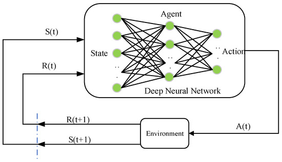
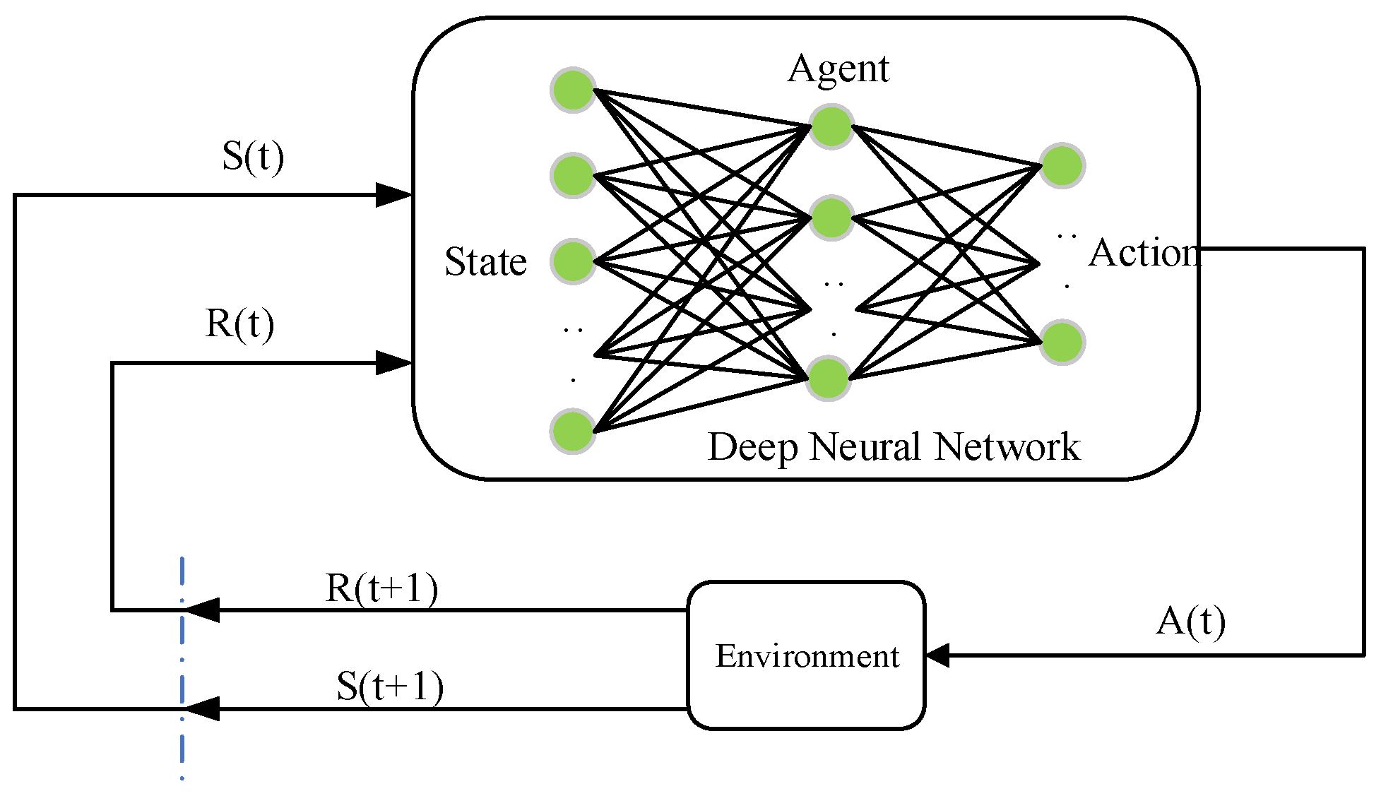
This study reframes the Integrated Energy System (IES) scheduling model within a Deep Reinforcement Learning (DRL) framework, thereby formulating it as a sequential decision-making problem. The Trust Region Policy Optimization (TRPO) algorithm is employed to allow an agent to autonomously discover a globally optimal scheduling strategy via its policy optimization mechanism. In this model, the entire IES serves as the interactive environment for the agent. The agent, in turn, achieves coordinated optimal scheduling by dynamically adjusting the operational states of the system’s components. The specific interaction process is shown in Figure 4.

Figure 4. Markov decision process.

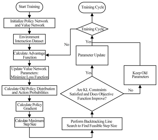
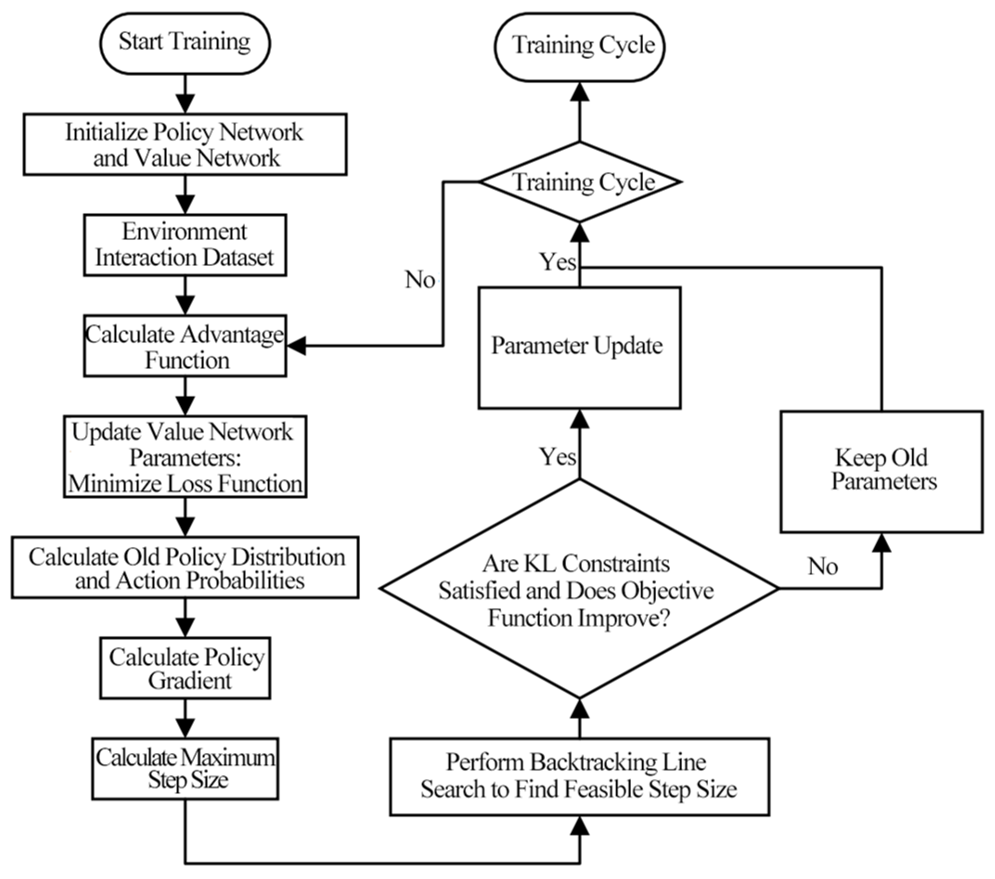
The Trust Region Policy Optimization (TRPO) algorithm is fundamentally based on Policy Gradient (PG) methods. The algorithm flow is shown in Figure 5.

Figure 5. Flowchart of TRPO algorithm.

The expected cumulative reward in the MDP is defined as:

$$\eta (\tilde{\pi })=E_{s_0,a_0,\cdots }\left[\sum _{t=0}^{\infty }{\gamma }^{t}r\left(s_t\right)\right]$$

(33)

The relationship between the performance of the new policy and the old policy is expressed as:

$$\eta (\tilde{\pi })=\eta (\pi )+E_{s_0,a_0,\cdots \sim \tilde{\pi }}\left[\sum _{t=0}^{\infty }{\gamma }^t{A}_{\pi }(s_t,a_t)\right]$$

(34)

where $E_{s_0,a_0,\cdots \sim \tilde{\pi }}\left[\cdot \cdot \cdot \right]$ denotes that the action is sampled according to the policy $a_t\sim \tilde{\pi }\left(·|s_t\right)$.

By expanding the expression for the expected cumulative discounted advantage of the old policy, Equation (17) can be reformulated as Equation (18).

$$\eta (\tilde{\pi })=\eta (\pi )+\sum _{t=0}^{\infty }\sum _{s}P(s_t=s|\tilde{\pi })\sum _a\tilde{\pi }(a|s){\gamma }^t{A}_{\pi }(s,a)$$

(35)

Focusing solely on the action distribution and holding other variables constant, this term represents a summation over the entire action space for a given state.

Let ${\rho }_{\pi }$ represent the discounted visitation frequency for state $s$:

$${\rho }_{\pi }(s)=P(s_0=s)+\gamma P(s_1=s)+{\gamma }^{2}P(s_2=s)+\cdot \cdot \cdot$$

(36)

where ${\rho }_0$ is the probability distribution of the initial state $s_0$, and all subsequent actions are selected according to the policy $\pi$. Given these definitions, Equation (20) can be rewritten as:

$$\begin{array}{cc}\eta (\tilde{\pi })\hfill & =\eta (\pi )+{\displaystyle \sum _{t=0}^{\infty }}{\displaystyle \sum _s}P(s_t=s|\tilde{\pi }){\displaystyle \sum _a}\tilde{\pi }(a|s){\gamma }^t{A}_{\pi }(s,a)\hfill \\ & =\eta (\pi )+{\displaystyle \sum _s}{\displaystyle \sum _{t=0}^{\infty }}{\gamma }^{t}P(s_t=s|\tilde{\pi })\sum _a\tilde{\pi }(a|s)A_{\pi }(s,a)\hfill \\ & =\eta (\pi )+{\displaystyle \sum _s}{\rho }_{\tilde{\pi }}(s){\displaystyle \sum _a}\tilde{\pi }(a|s)A_{\pi }(s,a)\hfill \end{array}$$

(37)

The dependence of the discounted state visitation frequency ${\rho }_{\tilde{\pi }}(s)$ on the unknown target policy $\tilde{\pi }$ renders the direct optimization of Equation (18) intractable. Therefore, the algorithm instead optimizes a local approximation of the performance objective $\eta (\tilde{\pi })$:

$$L_{\pi }(\tilde{\pi })=\eta (\pi )+\sum _s{\rho }_{\pi }(s)\sum _a\tilde{\pi }(a\mid s)A_{\pi }(s,a)$$

(38)

During a policy update, if the expected advantage is non-negative for every state, then the performance objective is guaranteed to be monotonically non-decreasing. This ensures that the performance after each update will either improve or remain the same.

In the TRPO algorithm, discrepancies in the action distribution can adversely affect performance during policy updates. To address this, Importance Sampling (IS) is employed to effectively manage the action distribution. IS is a statistical method primarily used to estimate expected values. Its core utility is realized in situations where sampling directly from a target probability distribution is infeasible. IS resolves this by using samples drawn from a different, known probability distribution and re-weighting them to correct for the mismatch.

The TRPO algorithm imposes a constraint on the KL divergence between the new and old policies, known as the trust region constraint. This approach reframes the original objective into a constrained optimization problem. By doing so, it effectively addresses the issue of suboptimal step sizes that can arise from using a simple penalty factor, thus leading to more stable algorithm performance. The problem is formulated as maximizing the objective $\max L_{{\theta }_{\mathrm{old}}}(\theta )$ while satisfying the constraint $D_{KL}^{\max }[{\theta }_{\mathrm{old}},\theta ]\le \delta$, where the constraint is defined using the mean KL divergence:

$${\overline{D}}_{KL}^{\rho }({\theta }_1,{\theta }_2)=E_{s~p}\left[D_{KL}\left({\pi }_{{\theta }_1}\left(·\mid s\right)\Vert {\pi }_{{\theta }_2}\left(·\mid s\right)\right)\right]$$

(39)

When approximating the constraint using the maximum KL divergence, the condition is modified to: ${\overline{D}}_{KL}^{{\rho }_{{\theta }_{\mathrm{old}}}}({\theta }_{\mathrm{old}},\theta )\le \delta$.

After expanding $L_{{\theta }_{\mathrm{old}}}(\theta )$, the objective function can be rewritten as:

$${\max }_{\theta }{\displaystyle \sum _s{\rho }_{\mathrm{old}}}(s){\displaystyle \sum _a{\pi }_{\theta }}(a\mid s)A_{\mathrm{old}}(s,a)$$

(40)

where $q$ denotes the probability distribution used for sampling.

In summary, the final optimization problem for the Trust Region Policy Optimization (TRPO) algorithm can be formulated as follows:

$$\underset{\theta }{\max }{E}_{s\sim {\rho }_{{\theta }_{\mathrm{old}}}},a\sim q\left[{\displaystyle \frac{{\pi }_{\theta }(a\mid s)}{q(a\mid s)}}{Q}_{{\theta }_{\mathrm{old}}}(s,a)\right]$$

(41)

Subject to $E_{s\sim {\rho }_{{\theta }_{\mathrm{old}}}}[D_{KL}({\pi }_{{\theta }_{\mathrm{old}}}(·|s)\parallel {\pi }_{\theta }(·|s))\le \delta ]$. Two primary sampling methods are commonly employed: the single-path method and the multi-path method. The single-path method is widely applied in scenarios involving infinite-horizon policy gradient estimation, whereas the multi-path method is more frequently used in the context of policy iteration. Specifically, the single-path method is tailored for gradient estimation over an infinite horizon, while the multi-path method is designed to support the continuous policy updates inherent in policy iteration. Thus, each approach addresses the distinct requirements of different algorithm designs and problem-solving contexts.

The parameters have been updated as follows:

$$g={\nabla }_{\theta }\mathbb{E}\left[\log {\pi }_{\theta }(a\mid s)\cdot A_t\right]$$

(42)

$$H\cdot x=g$$

(43)

$${\theta }_{\mathrm{new}}={\theta }_{\mathrm{old}}+\alpha \cdot x$$

(44)

where $H$ is the second-order derivative matrix of the KL divergence.

4.1. State Space

In the IES scheduling optimization model, the state space must accurately represent the system’s operational environment. It is therefore composed of key variables including the demand-side load, electricity price, natural gas price, and the power output from renewable energy sources. The state space is formally defined as follows:

$$\begin{array}{l}{S}_t^{\mathrm{e}}=\left[\begin{array}{c}{L}_{\mathrm{e}}^t,L_{\mathrm{h}}^t,L_{\mathrm{q}}^t,f_{\mathrm{wt}}^t,f_{\mathrm{pv}}^t,{\kappa }_{\mathrm{grid}}^t\end{array}\right]\\ S_t^{\mathrm{s}}=\left[P_{\mathrm{chp}}^t,H_{\mathrm{gb}}^t,Q_{\mathrm{p}2\mathrm{g}}^t\right]\end{array}$$

(45)

Based on the nature of the variables in the Integrated Energy System, the state space is partitioned into two components: the environmental state and the policy state. The environmental state encompasses external, uncontrollable variables, while the policy state represents the internal status of the system’s controllable assets.

4.2. Action Space

The action space is designed to encompass all controllable decision variables within the system. These variables include the power output of the GT, the thermal power output of the gas boiler, the power consumption of the Power-to-Gas (P2G) equipment, the electrical power purchased from the main grid, and the rate of natural gas procured from the main gas network. The complete action space is formally defined in Equation (26) as:

$$A_t=\left[\begin{array}{c}{Q}_{\mathrm{CHP}}^t,P_{\mathrm{P}2\mathrm{G}}^t,Q_{\mathrm{GB}}^t,P_{buy}^t,Q_{buy}^t,H_{buy}^t\end{array}\right]$$

(46)

The system variables in the proposed model exhibit temporal coupling characteristics, which makes it difficult to satisfy the energy balance constraints when using the action space defined in Equation (26). To reduce the model’s complexity and address this challenge, the action space is redefined. The new action space consists of the energy inputs to the components: the gas consumption of the gas boiler, the electricity consumption of the Power-to-Gas (P2G) equipment, and the gas consumption of the GT. This revised formulation is presented in Equation (27):

$$A_t=\left[\begin{array}{c}{Q}_{\mathrm{CHP}}^t,P_{\mathrm{P}2\mathrm{G}}^t,Q_{\mathrm{GB}}^t\end{array}\right]$$

(47)

4.3. Reward Function

The PIES scheduling optimization in this study is defined by three core objectives: minimizing economic cost, minimizing carbon emissions, and maximizing exergy efficiency. A primary challenge is that these objectives have disparate units of measurement, making direct comparison and trade-offs difficult. To address this, we employ the Technique for Order of Preference by Similarity to Ideal Solution (TOPSIS) method to construct a multi-objective reward function. This approach enables a comprehensive and balanced evaluation of the different goals.

4.3.1. Similarity to the Ideal Solution

The Technique for Order of Preference by Similarity to Ideal Solution (TOPSIS) is a widely used multi-criteria evaluation method. It leverages the information in the raw data to produce results that accurately reflect the performance differences between alternatives. The core principle of TOPSIS is to find an optimal compromise solution by assessing the proximity of each alternative to both a positive-ideal solution and a negative-ideal solution. The implementation of the TOPSIS method involves the following two steps:

• Normalization

Since the three optimization objectives have disparate units, the raw data matrix must first be pre-processed. The initial step is to unify the indicator types by converting any “cost” criteria into “benefit” criteria. Subsequently, this transformed matrix is normalized to eliminate the influence of the different measurement scales. This normalized decision matrix is then used to determine the Positive-Ideal Solution and the Negative-Ideal Solution.

$$z_t^i={\displaystyle \frac{x_t^i-x_{\min }^i}{x_{\max }^i-x_{\min }^i}}$$

(48)

where $z_t^i$ denotes the normalized value of the $i$-th target at time $t$; $x_t^i$ denotes the value of the $i$-th target before normalization at time $t$; $x_{\min }^i$ and $x_{\max }^i$ represent the minimum and maximum values of the i-th target, respectively.

After normalizing the three target values, the following scheduling plan can be obtained:

$$Z_t=\left[S_t,C_t,F_t\right]$$

(49)

where $z_t^i$ represents the optimal solution at time $t$; $F_t,C_t,S_t$ represent the economic efficiency target, carbon emission target, and energy efficiency target at time $t$, respectively.

2.

Calculating Distances to the Ideal Solutions

Each alternative, represented by its vector of normalized indicators, can be conceptualized as a point in a three-dimensional space. The Euclidean distance is then calculated between each alternative’s point and the points corresponding to the Positive-Ideal Solution and the Negative-Ideal Solution.

Based on the multi-objective optimization in the text—which prioritizes maximum efficiency, greatest carbon emission benefits, and lowest operating costs—the coordinates of the optimal and suboptimal solutions in the three-dimensional coordinate system are (0, 1, 0) and (1, 0, 1), respectively.

The operational plan obtained by the system can be calculated in normalized three-dimensional space based on the coordinates of the optimal and worst solutions within that space. This calculation yields the relative distances between Operational Plan A and both the optimal and worst solutions in the three-dimensional target space.

$$\left\{\begin{array}{l}{D}_t^{+}=\sqrt{{\left(z_t^1\right)}^2+{\left(z_t^2-1\right)}^2+{\left(z_t^3\right)}^2}\hfill \\ D_t^{-}=\sqrt{{\left(z_t^1-1\right)}^2+{\left(z_t^2\right)}^2+{\left(z_t^3-1\right)}^2}\hfill \end{array}\right.$$

(50)

where $D_t^{+}$ and $D_t^{-}$ represent the distances from this solution to the optimal solution and the worst solution at time $t$, respectively.

4.3.2. Reward Function

In the normalized three-dimensional objective space, the quality of a given solution is determined by its proximity to the Positive-Ideal Solution (PIS) and its distance from the Negative-Ideal Solution (NIS). A superior solution is one that is closer to the PIS and farther from the NIS. Based on this principle, the distances to these two ideal points are used to construct the reward function, which guides the agent’s learning process.

$$r_t={\displaystyle \frac{D^{-}}{D^{-}+D^{+}}}$$

(51)

In the multi-objective scheduling problem for the Integrated Energy System, the reward function must guide the agent to maximize its objective while adhering to all operational constraints. To this end, penalty terms for constraint violations are incorporated into the reward signal. The fundamental purpose of these penalty terms is to ensure strict compliance with all physical constraints, such as energy balance and equipment ramp rates. They serve as mandatory safeguards rather than trade-offs between different feasible solutions.

$$R_t={\alpha }_1{r}_t+{\alpha }_2{C}_{F,t}$$

(52)

where ${\alpha }_1$, ${\alpha }_2$ are the scaling coefficients for the objective function term and the constraint penalty term, respectively, in the reward function at time step $t$; $C_{F,t}$ is the value of the constraint penalty.

5. Simulation and Results

5.1. Verification of Advantages Considering CCS Under a Stepwise Carbon Trading Mechanism

5.1.1. Simulation Parameters

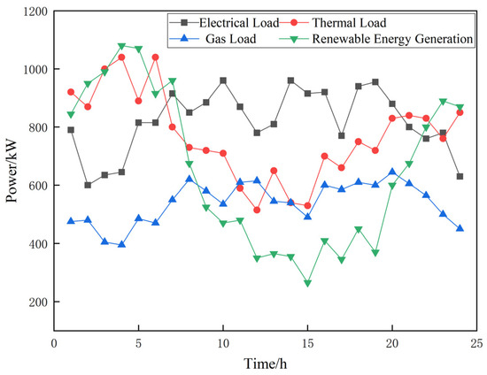
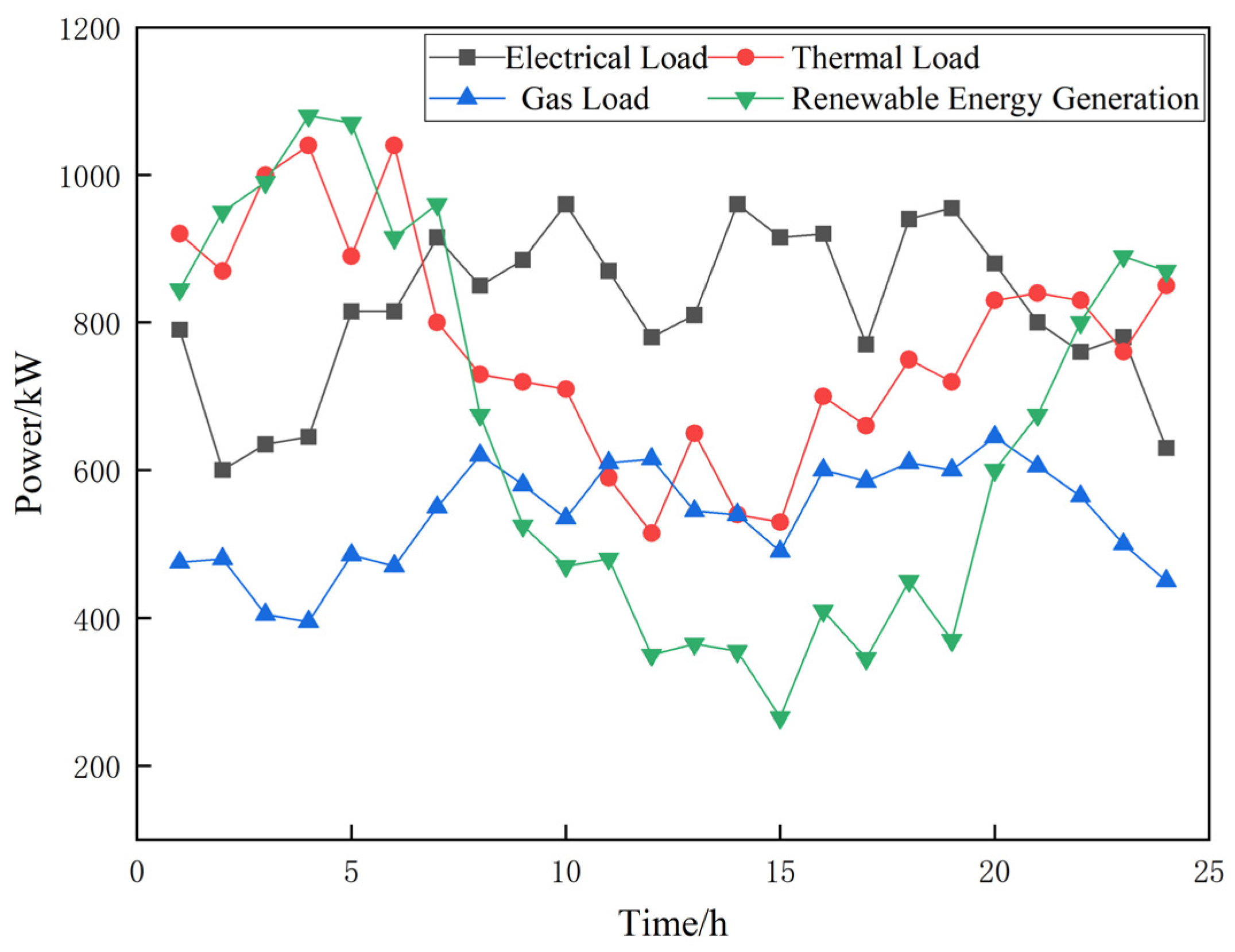
This section selects a comprehensive energy system demonstration park in Tianjin, China as the research subject, employing a 24 h scheduling cycle for simulation analysis. Figure 6 displays the typical daily electricity, heat, and gas load curves alongside wind power generation output for the park. Table 1 lists the time-of-use electricity prices and natural gas market prices, while Table 2 details the capacity configurations and technical parameters of each energy conversion device within the system. Additional relevant parameters are specified in Table 3.

Figure 6. Electricity/gas/heat loads and renewable energy outputs in the PIES.

Table 1. Time-of-use electricity price, natural gas price.

Parameters	Price (CNY/kWh)	Price (CNY/kWh)
$c_{\mathrm{fs}}(t)$	00:00–07:00, 22:00–24:00	0.4
	07:00–11:00, 14:00–18:00	0.8
	11:00–14:00, 18:00–22:00	1.20
$c_{\mathrm{fs}}(t)$	00:00–24:00	0.35

Table 2. Equipment parameters of Verification of Advantages Considering CCS Under a Stepwise Carbon Trading Mechanism.

Equipment	Capacity/kW	Conversion Efficiency/%	Ramping Rate/kW
P2G System	2000	60	400
GT	1400	Electric: 35 Thermal: 45	160
GB	1000	82	200
WHB	360	80	/

Table 3. Other parameters.

Parameter	Parameter Value	Parameter	Parameter Value
${\chi }_{\mathrm{e}}^{*}/\left[\mathrm{kg}\cdot {(\mathrm{kW}\cdot \mathrm{h})}^{-1}\right]$	0.728	$\alpha /\left(\mathrm{kw}\cdot {\mathrm{kg}}^{-1}\right)$	0.8333
${\chi }_{\mathrm{h}}^{*}/\left[\mathrm{kg}\cdot {(\mathrm{kW}\cdot \mathrm{h})}^{-1}\right]$	0.234	$\beta$	80%
${\chi }_{\mathrm{e}}/\left[\mathrm{kg}\cdot {(\mathrm{kW}\cdot \mathrm{h})}^{-1}\right]$	1.08	$\lambda /\left(\mathrm{CNY}\right.\left.\cdot {\mathrm{kg}}^{-1}\right)$	0.47
${\chi }_{\mathrm{h}}/\left[\mathrm{kg}\cdot {(\mathrm{kW}\cdot \mathrm{h})}^{-1}\right]$	0.367	$P_{\mathrm{buv}}^{\max }/\mathrm{kW}$	600
${\chi }_{\mathrm{g}}^{*}/\left[\mathrm{kg}\cdot {(\mathrm{kW}\cdot \mathrm{h})}^{-1}\right]$	0.18	$G_{\mathrm{buv}}^{\max }/\mathrm{kW}$	1150
${\chi }_{\mathrm{g}}/\left[\mathrm{kg}\cdot {(\mathrm{kW}\cdot \mathrm{h})}^{-1}\right]$	0.2	$\mu$	0.25
$\gamma$	1.67	$l/\mathrm{kg}$	400
$\psi /\left(\mathrm{CNY}\right.\left.\cdot {\mathrm{kg}}^{-1}\right)$	0.25

5.1.2. Comparison Scenarios

This section employs Equations (1) through (17) and Equations (24) through (32) to establish a mixed-integer linear programming model, utilizing the CPLEX solver for computation.

Scenario 1 [27]: Under the traditional carbon trading mechanism, consider the PIES low-carbon economic optimization operation model incorporating carbon capture equipment.

Scenario 2 [28]: Low-carbon economic optimization operation model for PIESs under a stepwise carbon trading mechanism, excluding carbon capture equipment.

Scenario 3: Under a tiered carbon trading mechanism, consider the PIES low-carbon economic optimization operation model incorporating carbon capture equipment.

5.1.3. Results Analysis

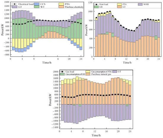
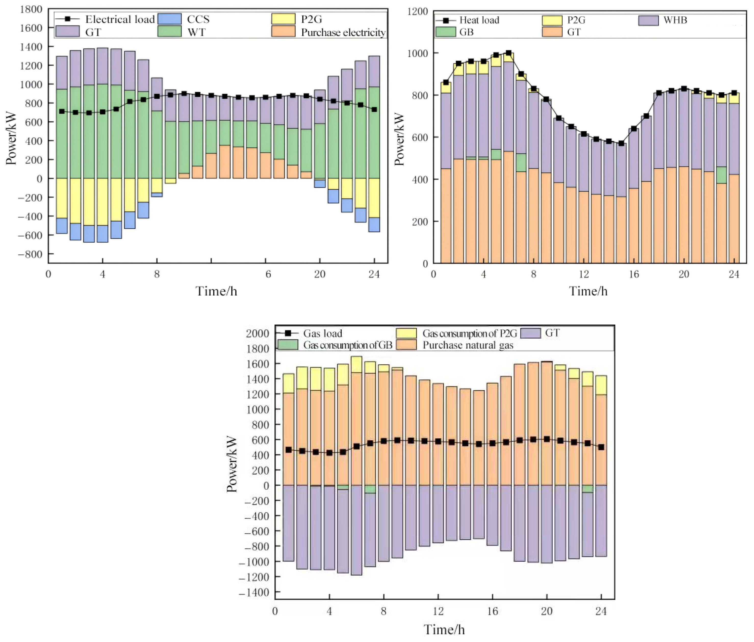
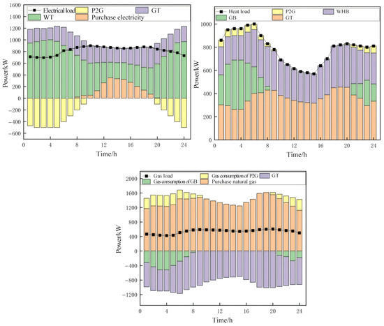
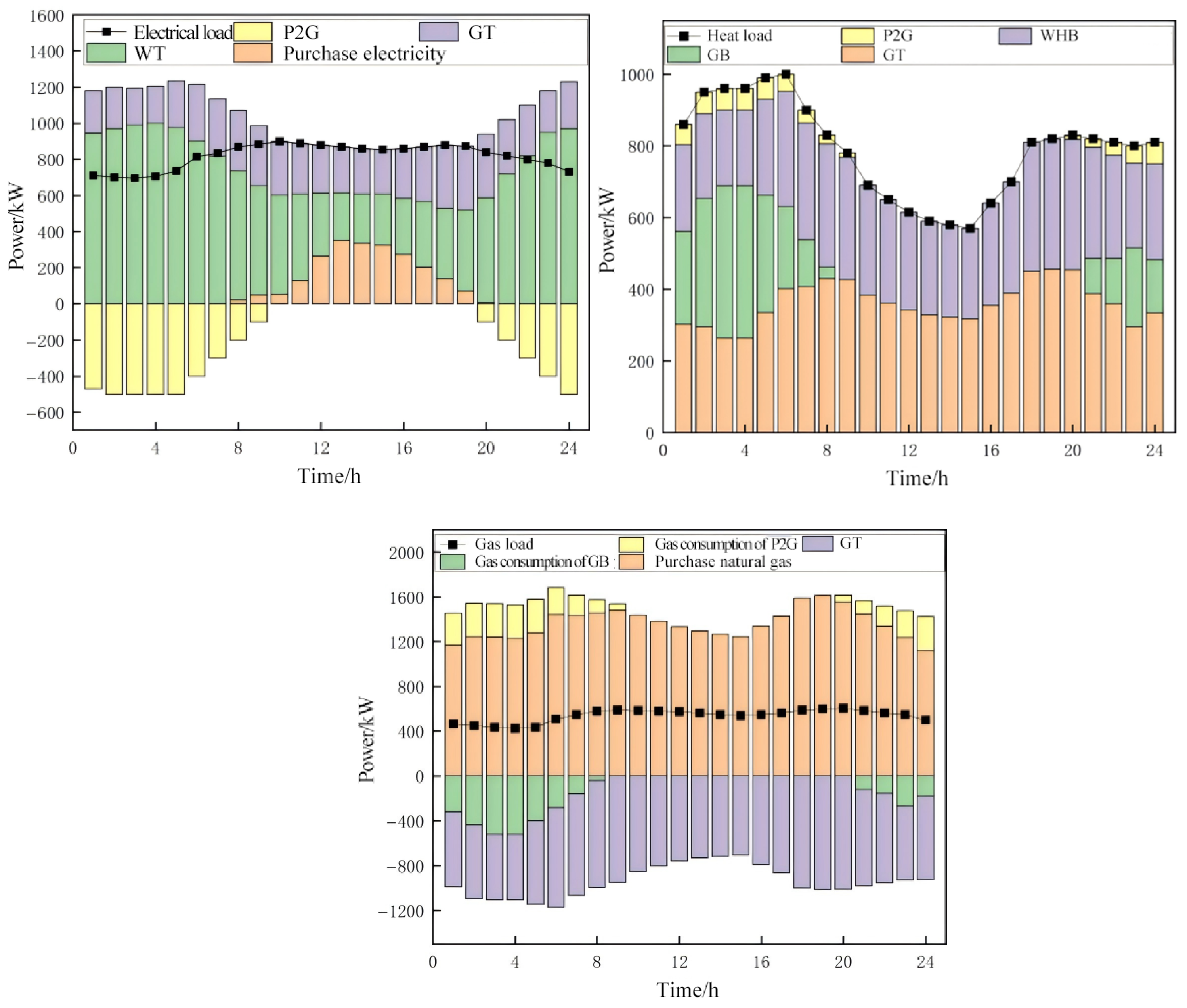
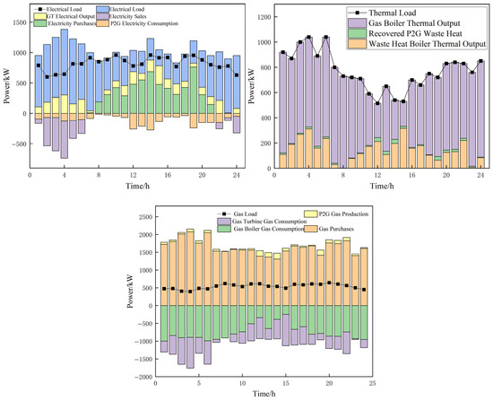
The scheduling results are shown in Figure 7 and Figure 8. This study evaluates the practical application effectiveness of carbon capture technology within integrated energy systems through comparative experimental design. Specifically, under a tiered carbon pricing policy framework, two scenarios were established for comparative analysis: one incorporating carbon capture equipment (Scenario 3) and another excluding it (Scenario 2). This approach verifies the dual role of carbon capture technology in enhancing both the environmental benefits and operational economics of the system.

Figure 7. Power/heat/gas balance diagrams for carbon-containing capture equipment in PIES.

Figure 8. Electrical/heat/gas power balance of PIES without carbon capture equipment.

As shown in Table 4, Scenario 2 incurs lower energy procurement costs than Scenario 3 since it avoids operational electricity expenses for carbon capture equipment. However, this scenario entails significant environmental trade-offs: First, all CO₂ emissions from gas turbines and boilers are directly released, resulting in higher carbon trading costs than Scenario 3. Second, the inability to utilize carbon resources for sale eliminates potential revenue from CO₂ sales. Comprehensive calculations indicate that the total operating cost of Scenario 2 is actually higher than that of Scenario 3.

Table 4. Control Results.

Project Name	Scenario 1	Scenario 2	Scenario 3
Electricity Purchase Cost/CNY	1931.10	1815.29	2097.06
Gas Purchase Cost/CNY	10,745.43	9842.31	10,609.48
Wind Power Curtailment Penalty/CNY	0	0	0
Carbon Trading Cost/CNY	517.53	1152.51	304.23
CO2 Sales Profit/CNY	602.44	0	1168.23
Purchased CO2 Cost/CNY	0	11.85	0
Actual carbon emissions/kg	7983.33	9694.43	7561.05
Total Cost/CNY	12,591.62	12,821.96	11,842.54

From the perspective of operational flexibility, Scenario 3 demonstrates significant advantages: on one hand, internal carbon recycling eliminates the transportation and storage issues associated with externally procured synthesis gas feedstock; on the other hand, the carbon resource management capability provided by the carbon capture equipment enhances the system’s scheduling flexibility.

Quantitative analysis indicates that under a tiered carbon pricing mechanism, the system equipped with carbon capture equipment achieves 22.01% carbon emissions reduction and 7.6% cost savings. This result fully demonstrates the dual value of carbon capture technology in enhancing both the environmental and economic benefits of integrated energy systems, providing important reference for the optimized design of low-carbon energy systems.

This study conducted comparative validation by constructing optimization models under two distinct carbon trading mechanisms: Scenario 1 employs a traditional carbon pricing model, while Scenario 3 applies a tiered carbon trading mechanism. Both models account for the configuration of carbon capture equipment. Comparative data in Table 4 demonstrate that the tiered carbon trading mechanism induces significant changes in system operation strategies, specifically manifested as: (1) Reduced total system carbon emissions, indicating that the new pricing mechanism strengthens emission reduction incentives; (2) Increased carbon capture volumes to counter cost pressures from tiered pricing; (3) Carbon resource sales revenue surged by 93.9%, substantially improving system economics. These findings conclusively demonstrate that the tiered carbon trading mechanism not only guides systems toward carbon reduction but also generates additional revenue through carbon resource sales, achieving synergistic gains in ecological performance and economic output.

5.2. Based on the TRPO Algorithm

5.2.1. Simulation Parameters

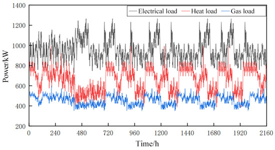
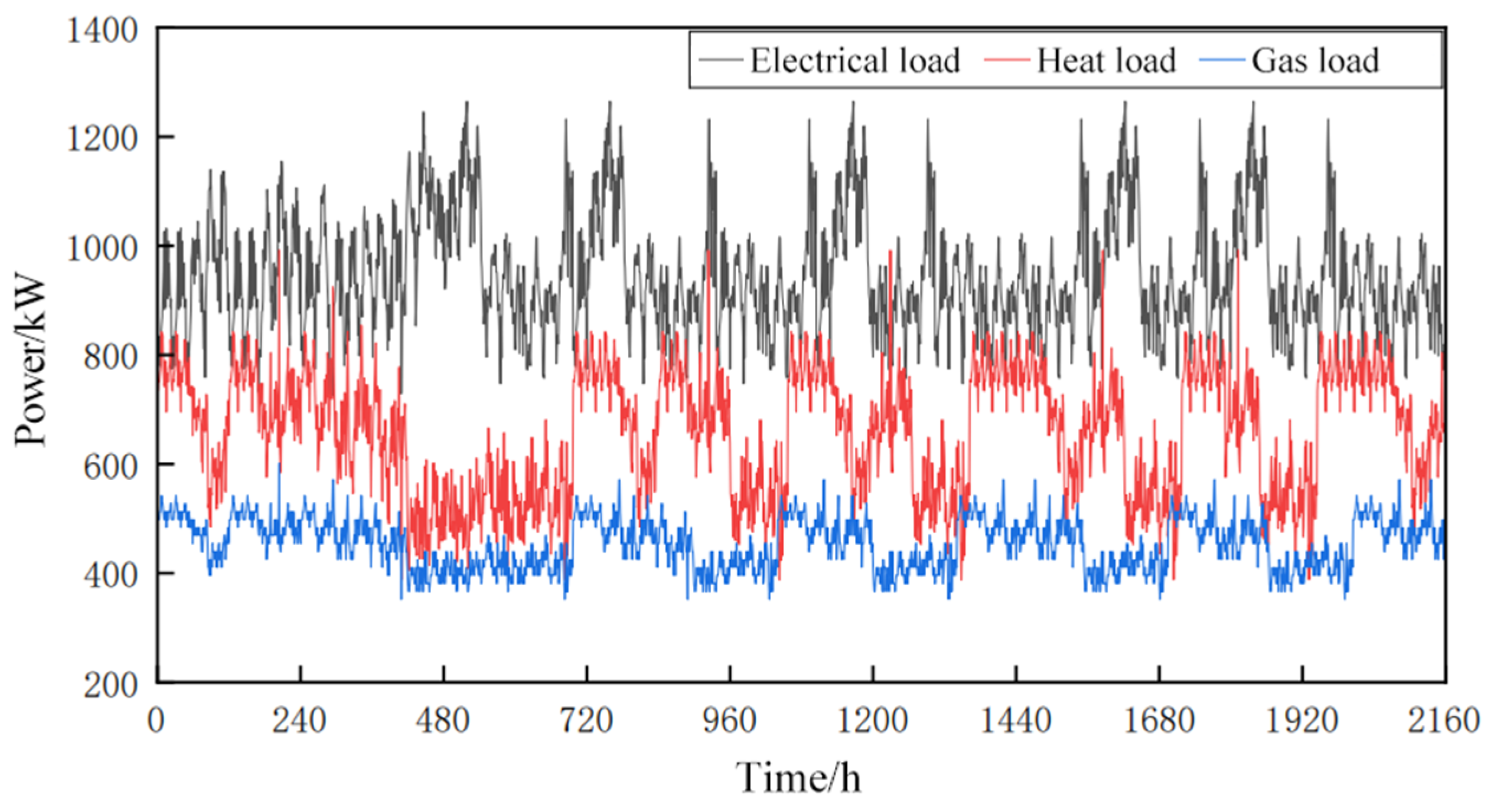
Figure 9 displays the internal wind power generation output of PIES, along with partial historical data for electricity, thermal energy, and gas loads. Time-of-use electricity and gas pricing information can be obtained from Table 1.

Figure 9. Historical data of electric/heat/gas loads in PIES.

The operational parameters for the system’s equipment are detailed in Table 5, and the actual carbon emission factors are listed in Table 6. The simulation also incorporates a Ladder-style carbon trading. The carbon emission allowance coefficients are set to 0.728 kg/(kW·h) for electricity generation from coal-fired units and 0.367 kg/(kW h) for thermal energy production from natural gas units. For direct natural gas consumption, the allowance is 0.180 kg/(kW·h). The carbon market is defined by a base price of 0.252 CNY/kg, with an emission bracket size of 2000 kg and a price escalation rate of 25% for each subsequent bracket. The parameters for the reinforcement learning algorithm are listed in Table 7. The network structure is shown in Table 8. The parameters for the Particle Swarm Optimization (PSO) algorithm are set as follows: The population size is set to 50 to balance exploration and exploitation efficiency. The inertia weight adopts a linearly decreasing strategy from 0.9 to 0.4, ensuring global exploration in early stages and local refinement in later iterations. Both the cognitive coefficient and social coefficient are set to 2.0. The maximum number of iterations is 5000, with an early termination criterion triggered if the improvement in the global best solution remains below 1 × 10⁻⁶ for 200 consecutive iterations. A reflection boundary-handling mechanism is applied to redirect particles back into the feasible domain defined by system operational constraints, and particle velocities are clamped within ±20% of the variable range to prevent divergence. These parameter settings are based on standard PSO practices and tailored to the complexity of the scheduling problem to ensure effective convergence in this study.

Table 5. Equipment parameters.

Equipment	Capacity/kW	Conversion Efficiency/%	Ramping Rate/kW
P2G System	500	60	400
Gas Turbine	1400	Electric: 35 Thermal: 45	160
Gas Boiler	600	82	200
Waste Heat Boiler	360	80	/

Table 6. Carbon emission factors.

Parameter	Value
$\mathrm{Carbon} \mathrm{Emission} \mathrm{Factor} \mathrm{for} \mathrm{Electricity}/[\mathrm{t}·{(\mathrm{MW}·\mathrm{h})}^{-1}]$	1.08
$\mathrm{Carbon} \mathrm{Emission} \mathrm{Factor} \mathrm{for} \mathrm{Heat}/[\mathrm{t}·{\mathrm{GJ}}^{-1}]$	0.065
$\mathrm{Carbon} \mathrm{Emission} \mathrm{Factor} \mathrm{for} \mathrm{Natural} \mathrm{Gas}/[\mathrm{t}·{(\mathrm{MW}·\mathrm{h})}^{-1}]$	0.2
Electricity-to-Heat Conversion Ratio/$[\mathrm{MJ}·{(\mathrm{MW}·\mathrm{h})}^{-1}]$	6

Table 7. TRPO hyperparameter settings.

Parameter	Value
Max episodes	36,000
Max steps	24
$lr$	0.01
KL	0.00005
$\gamma$	0.9
$\alpha$	0.5
Replay Buffer Size	1 × 106

Table 8. TRPO algorithm network parameters.

Project	Strategic Network	Value Network
Input layer neuron	5	5
Hidden Layer 1 Neuron	128	128
Hidden Layer 2 Neuron	128	128
Output layer neuron	3	1

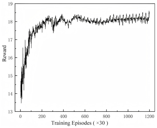
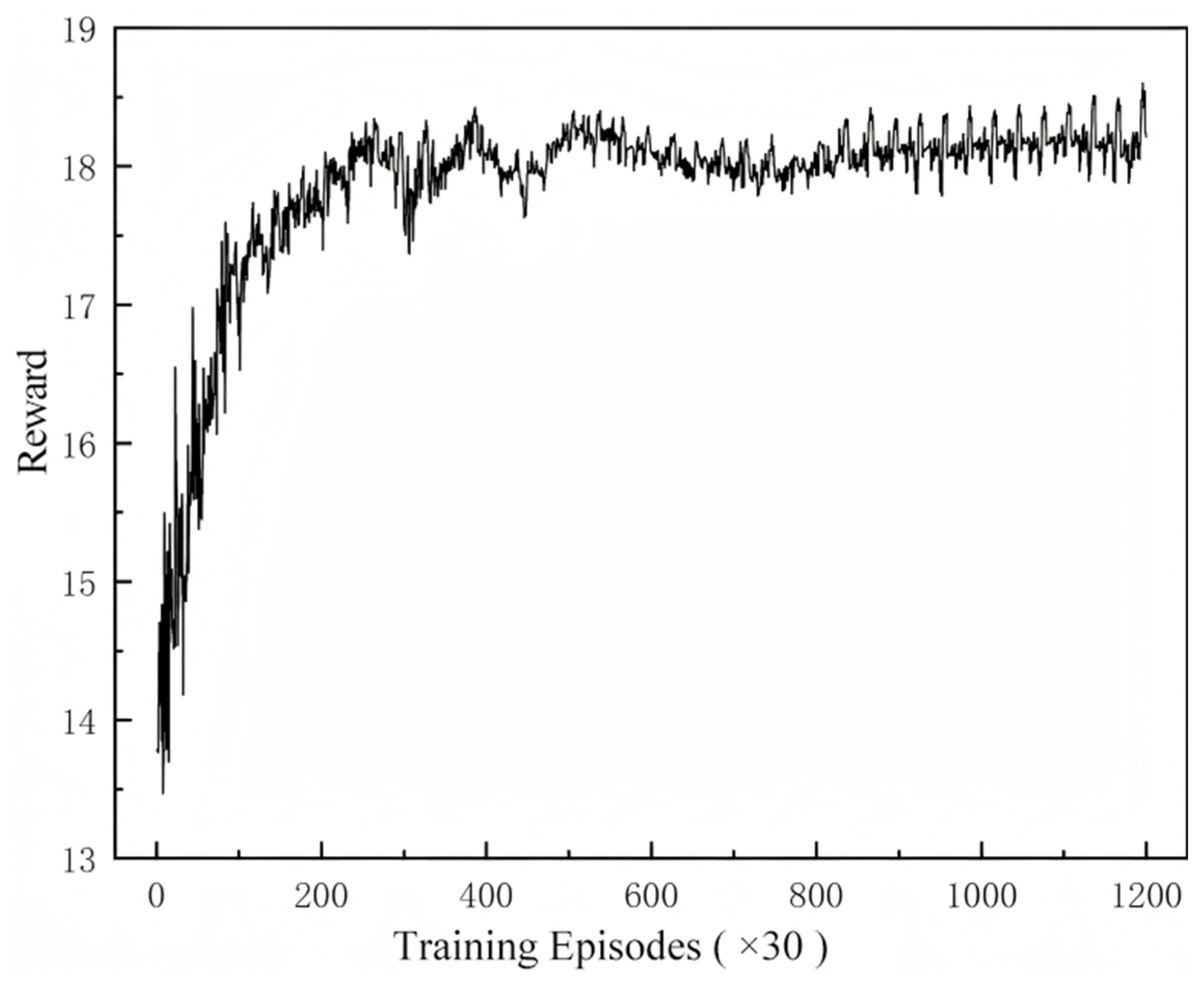
The TRPO algorithm requires an initial training phase before the agent is deployed for online application. This is a one-time offline process where the agent is trained on historical system data, and the resulting network is saved. For the case study in this paper, a training set consisting of 90 days of historical data from a park-level energy system was used. The agent was trained for 36,000 episodes, and the corresponding reward curve is shown in Figure 10. The curve indicates that the agent’s performance converges at approximately the 700th episode.

Figure 10. Agent pre-training process.

The scheduling time step is set to one hour, defining a daily operational cycle of 24 time steps. The fluctuations observed in the reward curve are an expected outcome of the stochastic exploration mechanism, which is essential for the learning process. This mechanism introduces action noise to encourage exploration and prevent the agent from settling into a suboptimal local optimum.

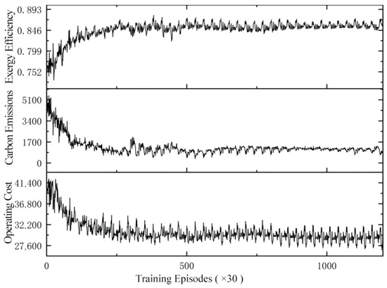
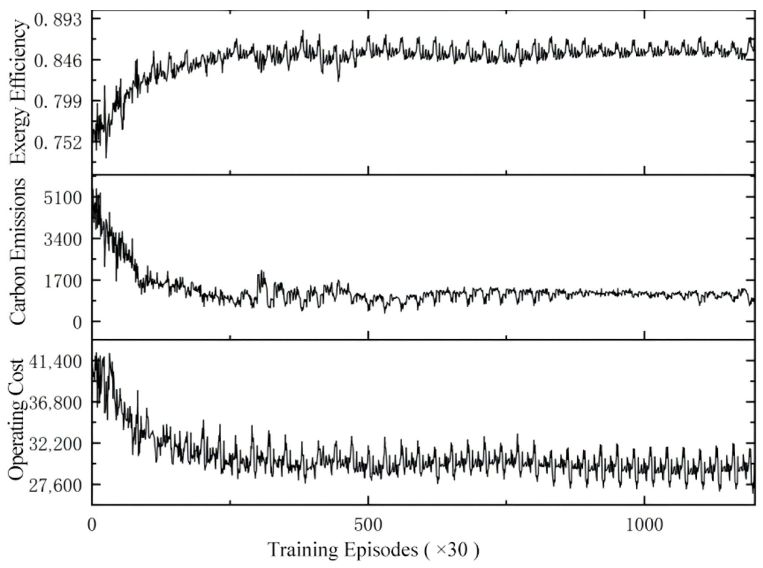
Figure 11 illustrates the learning progress for the three individual objectives: operating cost, carbon emissions, and exergy efficiency. During the initial 700 training episodes, all three metrics undergo significant changes. The operating cost initially fluctuates around 41,400 before converging to approximately 25,500. Carbon emissions exhibit a substantial reduction, dropping from 5100 to a stable value of around 1100. Concurrently, exergy efficiency improves from an average of 0.75 to a stable 0.85. Given that operating cost and carbon emissions are minimization objectives, while exergy efficiency is a maximization objective, these trends demonstrate effective optimization. The significant improvements in carbon performance and exergy efficiency, in particular, validate the effectiveness of the proposed method.

Figure 11. Multi-objective training process.

5.2.2. Results and Discussion

To evaluate the performance of the proposed method, it was compared with the DQN and PSO algorithms. Additionally, we employed the mixed-integer linear programming model, utilizing the CPLEX solver for computation (Model-based) as a theoretical optimality benchmark for comparison. In deep reinforcement learning studies or other model-free research, Model-based is frequently used to derive theoretically optimal solutions. To ensure a fair comparison between reinforcement learning methods, the DQN agent was trained using the same historical data and Markov Decision Process (MDP) model as the TRPO agent—including the state space, action space, and reward function. All parameters and network structures of the algorithms remain consistent.

Upon completion of the training phase, the trained model is saved. During online scheduling, this pre-trained model is loaded and utilized directly. The agent then processes real-time environmental data to determine the optimal scheduling decisions at each time step.

To validate the scheduling results of the proposed model, typical load days were randomly selected from historical data as test scheduling days. Specific data is shown in Figure 6.

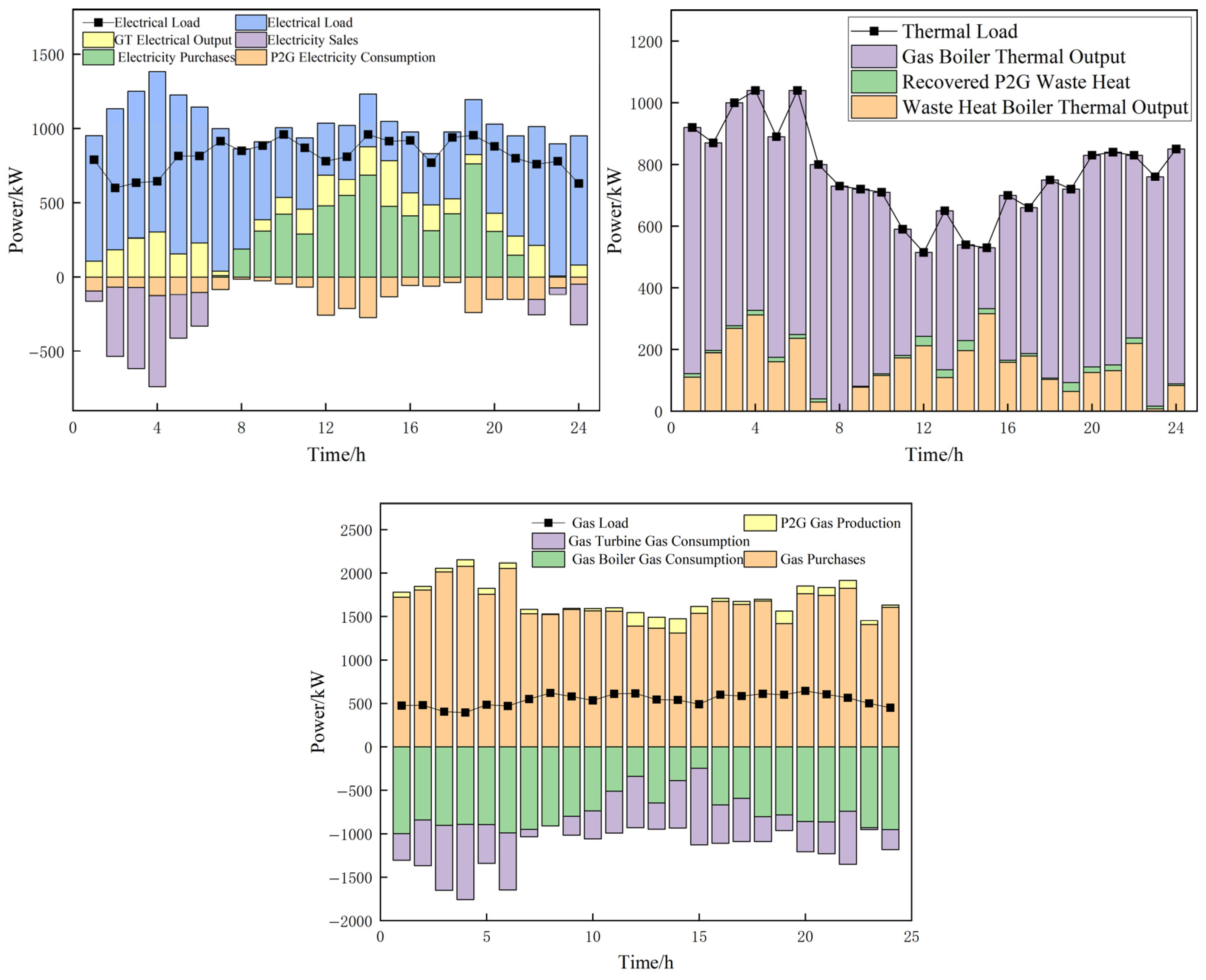
The power system dispatch results are presented in Figure 12. The system’s equipment dynamically adjusts its output strategy based on the load forecasts.

Figure 12. Multi-energy power balance constraints.

The learned policy demonstrates an intelligent dispatch strategy for high thermal load scenarios. The agent prioritizes the GB and WHB over the Combined Heat and Power (CHP) unit. This preference is driven by two key factors: the superior efficiency of GB and WHB for dedicated heat production and their significantly lower carbon emissions. Consequently, these units constitute the primary source of thermal energy during peak heating periods.

As illustrated in Figure 12, the dispatch logic is strongly influenced by the relative prices of electricity and natural gas. During peak and shoulder periods with high electricity tariffs, the system strategically increases natural gas consumption to minimize operational costs, keeping the Power-to-Gas (P2G) unit inactive as it is not economically viable. Conversely, during off-peak periods with low electricity prices, often coinciding with high renewable generation, the agent activates the P2G unit. This action enables the absorption of surplus renewable energy, converting it into storable gas to simultaneously reduce both operating costs and carbon emissions.

The comparative data in Table 9 clearly demonstrates the superior performance of our proposed TRPO method across all metrics. Solution time is the duration from the start of the test to the generation of the control strategy. Training Duration refers solely to the time spent on training and is typically not considered during the control process. The method proposed in this paper also approaches the theoretically optimal value. Compared to the solution from our TRPO approach, the DQN-based schedule resulted in 5.7% higher operating costs and carbon emissions, with a 5.3% reduction in exergy efficiency; the PSO algorithm performed even more poorly. This highlights that the compromise solution identified by our method is superior in terms of cost control, emissions reduction, and energy efficiency. This performance gap stems from the inherent characteristics of the algorithms: First, its direct policy optimization method is inherently suited for continuous action spaces, as it outputs continuous actions directly through a parameterized policy, thereby avoiding the curse of dimensionality and loss of precision that DQN suffers from due to the need for action discretization. Second, its core trust region constraint fundamentally ensures optimization stability by strictly limiting the step size of policy updates, effectively overcoming the training oscillations and collapses caused by DQN’s value estimation errors and policy overfitting. Finally, compared to model-free metaheuristic algorithms like PSO, TRPO possesses a rigorous policy gradient theoretical framework and guarantees monotonic improvement, thus avoiding the common issues of local optima and low search efficiency that PSO faces in complex high-dimensional problems. Therefore, TRPO theoretically provides a more stable and convergent optimization path for continuous control. In contrast, the TRPO algorithm operates directly in a continuous action space, giving it a natural adaptive advantage for the complex control tasks within an Integrated Energy System. Furthermore, its substantially higher computational efficiency compared to PSO meets the stringent timeliness requirements of real-time scheduling, establishing it as the preferred solution for online applications. It should be noted that while Model-based is theoretically optimal, its solution time is relatively long, so it may not meet the demand for rapid solutions in certain situations.

Table 9. Performance comparison of different methods.

Algorithm	Operating Cost/CNY	Carbon Emissions/kg	Exergy Efficiency/%	Solution Time/s	Training Duration/h
Model-based	22,103.98	906.15	86.3	15.67	\
PSO	25,597.03	1148.43	83.5	10.35	\
DQN	25,338.63	1073.34	84.9	0.98	5.3
TRPO	22,420.12	946.09	85.1	0.95	2.1

5.2.3. TPRO vs. PPO

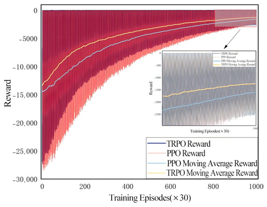
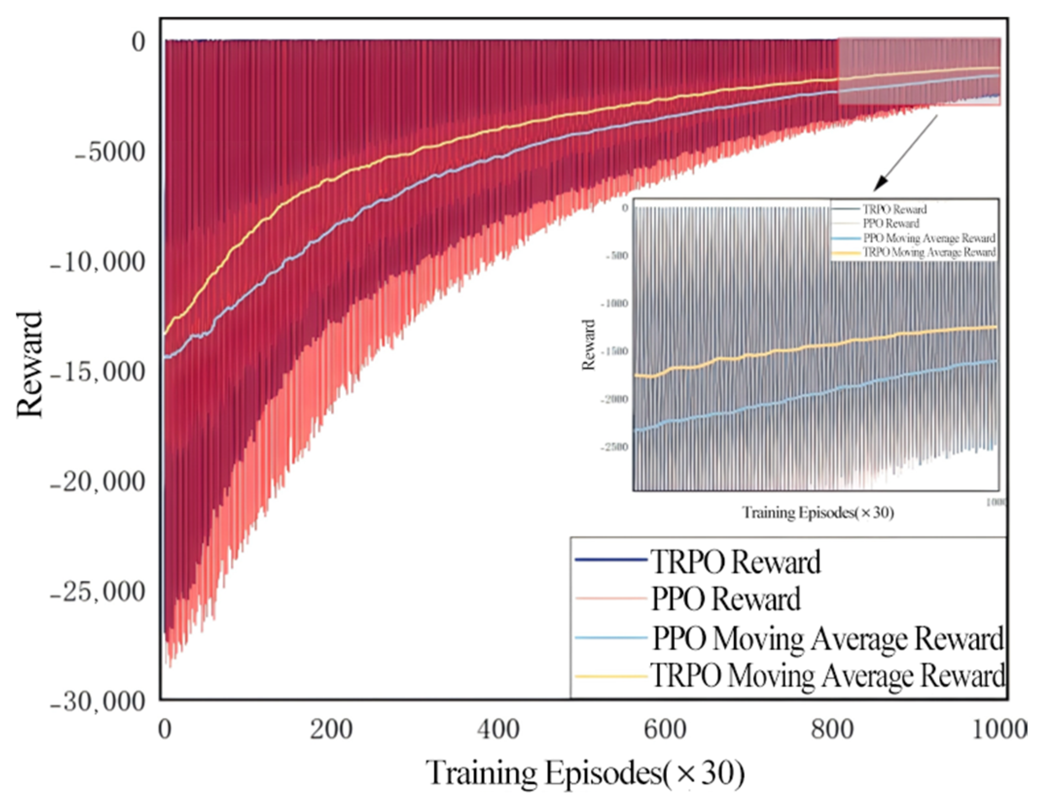
Since TPRO and PPO (Proximal Policy Optimization) are two closely related policy optimization algorithms in deep reinforcement learning, both belong to policy gradient methods and share the core idea of ensuring stability by constraining the step size of policy updates. However, PPO can be viewed as a simplified version of TPRO. Therefore, this paper compares TPRO and PPO within the PIES system. This subsection trains both methods using the same historical data. The training process is illustrated in Figure 13. Both methods converge around 800 epochs. The proposed algorithm in this chapter rapidly increases reward values during the early training phase compared to the PPO algorithm and converges to higher reward values.

Figure 13. Comparison of reward function curves during training.

The proposed algorithm demonstrates advantages in convergence value, convergence speed, and stability, with the shaded range indicating variance in experimental results. Within the initial 400 training epochs, the attention mechanism-based TRPO algorithm achieves faster reward growth compared to PPO, elevating the reward value from approximately −14,000 to around −5000. whereas the PPO algorithm only increased the reward value to around −7000 within 400 rounds. In the later training phase, around 800 rounds, the proposed algorithm converged, with the reward value stabilizing near −2600; the PPO algorithm showed slightly inferior performance compared to the proposed algorithm in both convergence speed and convergence value.

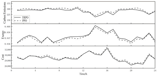
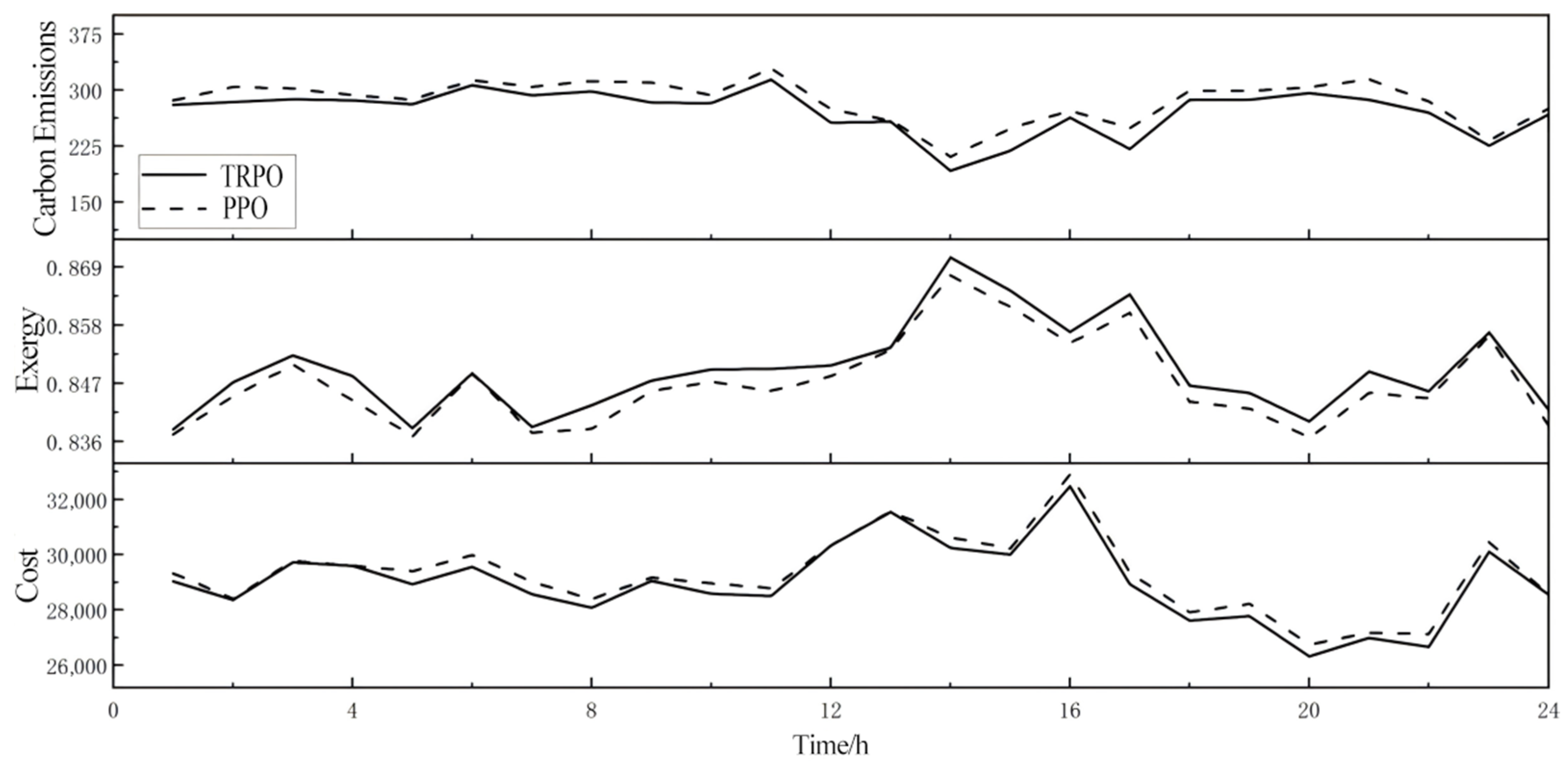
After training completion, the agents trained by both methods were saved. Subsequently, data from the same typical day was selected to validate the results of these two agents. Figure 14 presents the test results comparing the PPO algorithm with the proposed TRPO algorithm. Across evaluation metrics including operational costs, carbon emissions, and energy efficiency, the proposed TRPO algorithm demonstrates clear advantages over the PPO algorithm. This algorithm not only reduces system operating costs and carbon emissions but also effectively enhances energy efficiency.

Figure 14. Comparison of test results.

6. Conclusions and Prospects

This paper addressed the PIES optimization problem by proposing a low-carbon economic dispatch model based on the Trust Region Policy Optimization (TRPO) algorithm. The model was designed to achieve three primary objectives: minimizing operating costs, reducing carbon emissions, and maximizing exergy efficiency. The state and action spaces for the TRPO agent were carefully tailored to the system’s dynamic characteristics and operational constraints. The results of our analysis demonstrate that the TRPO algorithm can effectively leverage the high-dimensional historical data generated by the PIES. Compared to traditional heuristic algorithms, the proposed method significantly enhances the economic performance, environmental sustainability, and energy efficiency of the PIES in online scheduling applications.

Future research will focus on the following two key directions to further enhance the model’s accuracy, interpretability, and decision-support capabilities: (1) Research on High-Fidelity Equipment-Level Modeling and Data Fusion: To overcome the limitation of using constant efficiency coefficients for critical equipment such as P2G in the current study, future work will be dedicated to developing dynamic equipment models. (2) Development of a Decision Support System Based on Explicit Multi-Objective Optimization and Sensitivity Analysis: To investigate the sensitivity of objective weights and to improve the transparency and interpretability of scheduling strategies, the next step will involve constructing an explicit multi-objective decision support framework. This framework will treat cost, carbon emissions, and exergy efficiency as independent objectives. By employing multi-objective reinforcement learning algorithms or conditional policy optimization methods, it will systematically generate the Pareto optimal frontier for the PIES.

Additionally, while this work provides a promising prototype framework for intelligent scheduling in PIES, its industrial application remains constrained by challenges such as data dependency, security verification, generalization capabilities, and interpretability. Future research will focus on developing high-sample-efficiency training methods, algorithms with formal security guarantees, and meta-learning or adaptive mechanisms capable of adapting to environmental changes. Concurrently, we will explore human–machine collaborative decision-making models to progressively bridge the gap between simulation research and engineering practice.

References

- Laishram, T.; Bal, S. Energy transition: Paving the way for a greener future. Nanomater. Energy 2023, 12, 100–109. [Google Scholar] [CrossRef] [Scilit]
- Sun, Y.; Li, B.; Wang, Y.; Chen, K.; Tian, W. Flexibility Mining and Improvement for Urban Electricity-Gas-Heat-Storage Integrated Energy Systems: A Review. In Proceedings of the 2023 IEEE 7th Conference on Energy Internet and Energy System Integration (EI2), Hangzhou, China, 15–18 December 2023; IEEE: New York, NY, USA, 2023; pp. 913–919. [Google Scholar]
- Liu, C.; Li, Y.; Wang, Q.; Wang, X.; Chen, C.; Lin, Z.; Yang, L. Optimal configuration of park-level integrated energy system considering integrated demand response and construction time sequence. Energy Rep. 2022, 8, 1174–1180. [Google Scholar] [CrossRef] [Scilit]
- Yang, J.; Zeng, L.; He, K.; Gong, Y.; Zhang, Z.; Chen, K. Optimization of the Joint Operation of an Electricity–Heat–Hydrogen–Gas Multi-Energy System Containing Hybrid Energy Storage and Power-to-Gas–Combined Heat and Power. Energies 2024, 17, 3144. [Google Scholar] [CrossRef] [Scilit]
- Dong, X.; Jiang, C.; Liu, J.; Zhao, D.; Sun, B. Model predictive control optimization strategy for integrated energy systems: A two-stage dual-loop optimization framework. IEEE Trans. Sustain. Energy 2024, 15, 2234–2248. [Google Scholar] [CrossRef] [Scilit]
- Hu, J.; Zou, Y.; Soltanov, N. A multilevel optimization approach for daily scheduling of combined heat and power units with integrated electrical and thermal storage. Expert Syst. Appl. 2024, 250, 123729. [Google Scholar] [CrossRef] [Scilit]
- Liu, X.; Ji, Y.; Guo, Z.; Yuan, S.; Chen, Y.; Zhang, W. Study of Key Parameters and Uncertainties Based on Integrated Energy Systems Coupled with Renewable Energy Sources. Sustainability 2023, 15, 16266. [Google Scholar] [CrossRef] [Scilit]
- Martinez-Mares, A.; Fuerte-Esquivel, C.R. A robust optimization approach for the interdependency analysis of integrated energy systems considering wind power uncertainty. IEEE Trans. Power Syst. 2013, 28, 3964–3976. [Google Scholar] [CrossRef] [Scilit]
- Wang, Q.; Xiao, Y.; Tan, H.; Mohamed, M.A. Day-Ahead scheduling of rural integrated energy systems based on distributionally robust optimization theory. Appl. Therm. Eng. 2024, 246, 123001. [Google Scholar] [CrossRef] [Scilit]
- Chu, Y.; You, F. Model-based integration of control and operations: Overview, challenges, advances, and opportunities. Comput. Chem. Eng. 2015, 83, 2–20. [Google Scholar] [CrossRef] [Scilit]
- Cho, J.-H.; Wang, Y.; Chen, I.-R.; Chan, K.S.; Swami, A. A survey on modeling and optimizing multi-objective systems. IEEE Commun. Surv. Tutor. 2017, 19, 1867–1901. [Google Scholar] [CrossRef] [Scilit]
- Batalla-Bejerano, J.; Paniagua, J.; Trujillo-Baute, E. Energy market integration and electricity trade. Econ. Energy Environ. Policy 2019, 8, 53–68. [Google Scholar] [CrossRef] [Scilit]
- Ma, L.; Xie, L.; Ye, J.; Bian, Y. An Optimal Dispatch Strategy for Integrated Energy Systems in the Energy Market Environment. In Proceedings of the 2024 6th International Conference on Energy Systems and Electrical Power (ICESEP), Wuhan, China, 21–23 June 2024; IEEE: New York, NY, USA, 2024; pp. 321–327. [Google Scholar]
- Wang, Y.; Zheng, Y.; Yang, Q. Optimal energy management of integrated energy systems for strategic participation in competitive electricity markets. Energy 2023, 278, 127883. [Google Scholar] [CrossRef] [Scilit]
- Li, P.; Zhang, F.; Ma, X.; Yao, S.; Wu, Y.; Yang, P.; Zhao, Z.; Lai, L.L. Operation cost optimization method of regional integrated energy system in electricity market environment considering uncertainty. J. Mod. Power Syst. Clean Energy 2021, 11, 368–380. [Google Scholar] [CrossRef] [Scilit]
- Wu, G.; Yi, C.; Xiao, H.; Wu, Q.; Zeng, L.; Yan, Q.; Zhang, M. Multi-objective optimization of integrated energy systems considering renewable energy uncertainty and electric vehicles. IEEE Trans. Smart Grid 2023, 14, 4322–4332. [Google Scholar] [CrossRef] [Scilit]
- Meng, Q.; Xu, J.; Ge, L.; Wang, Z.; Wang, J.; Xu, L.; Tang, Z. Economic optimization operation approach of integrated energy system considering wind power consumption and flexible load regulation. J. Electr. Eng. Technol. 2024, 19, 209–221. [Google Scholar] [CrossRef] [Scilit]
- Wang, Y.; Wang, X.; Yu, H.; Huang, Y.; Dong, H.; Qi, C.; Baptiste, N. Optimal design of integrated energy system considering economics, autonomy and carbon emissions. J. Clean. Prod. 2019, 225, 563–578. [Google Scholar] [CrossRef] [Scilit]
- Jiao, P.; Cai, X.; Wang, L.; Chen, J.; Zhao, Y.; Cao, Y. Flexibility operation for integrated energy system considering hydrogen energy under inertia characteristics and stepped carbon trading mechanism. Sustain. Cities Soc. 2023, 98, 104809. [Google Scholar] [CrossRef] [Scilit]
- Lu, R.; Hong, S.H. Incentive-based demand response for smart grid with reinforcement learning and deep neural network. Appl. Energy 2019, 236, 937–949. [Google Scholar] [CrossRef] [Scilit]
- Li, Y.; Hu, X.; Zhuang, Y.; Gao, Z.; Zhang, P.; El-Sheimy, N. Deep reinforcement learning (DRL): Another perspective for unsupervised wireless localization. IEEE Internet Things J. 2019, 7, 6279–6287. [Google Scholar] [CrossRef] [Scilit]
- Biswas, A.; Acquarone, M.; Wang, H.; Miretti, F.; Misul, D.A.; Emadi, A. Safe reinforcement learning for energy management of electrified vehicle with novel physics-informed exploration strategy. IEEE Trans. Transp. Electrif. 2024, 10, 9814–9828. [Google Scholar] [CrossRef] [Scilit]
- Liang, Z.; Chung, C.Y.; Zhang, W.; Wang, Q.; Lin, W.; Wang, C. Enabling high-efficiency economic dispatch of hybrid AC/DC networked microgrids: Steady-state convex bi-directional converter models. IEEE Trans. Smart Grid 2024, 16, 45–61. [Google Scholar] [CrossRef] [Scilit]
- Xiong, L.-L.; Mao, S.; Tang, Y.; Meng, K.; Dong, Z.-Y.; Qian, F. Reinforcement learning based integrated energy system management: A survey. Acta Autom. Sin. 2021, 47, 2321–2340. [Google Scholar]
- Yi, Z.; Luo, Y.; Westover, T.; Katikaneni, S.; Ponkiya, B.; Sah, S.; Mahmud, S.; Raker, D.; Javaid, A.; Heben, M.J.; et al. Deep reinforcement learning based optimization for a tightly coupled nuclear renewable integrated energy system. Appl. Energy 2022, 328, 120113. [Google Scholar] [CrossRef] [Scilit]
- Liang, T.; Zhang, X.; Tan, J.; Jing, Y.; Lv, L. Deep reinforcement learning-based optimal scheduling of integrated energy systems for electricity, heat, and hydrogen storage. Electr. Power Syst. Res. 2024, 233, 110480. [Google Scholar] [CrossRef] [Scilit]
- Liang, T.; Chai, L.; Tan, J.; Jing, Y.; Lv, L. Dynamic optimization of an integrated energy system with carbon capture and power-to-gas interconnection: A deep reinforcement learning-based scheduling strategy. Appl. Energy 2024, 367, 123390. [Google Scholar] [CrossRef] [Scilit]
- Li, F.; Liu, L.; Yu, Y. Deep reinforcement learning-based multi-objective optimization for electricity–gas–heat integrated energy systems. Expert Syst. Appl. 2025, 262, 125558. [Google Scholar] [CrossRef] [Scilit]
- Li, Y.; Ma, W.; Li, Y.; Li, S.; Chen, Z.; Shahidehpour, M. Enhancing cyber-resilience in integrated energy system scheduling with demand response using deep reinforcement learning. Appl. Energy 2025, 379, 124831. [Google Scholar] [CrossRef] [Scilit]
- Chen, L.; He, H.; Jing, R.; Xie, M.; Ye, K. Energy management in integrated energy system with electric vehicles as mobile energy storage: An approach using bi-level deep reinforcement learning. Energy 2024, 307, 132757. [Google Scholar] [CrossRef] [Scilit]
- Coraci, D.; Brandi, S.; Hong, T.; Capozzoli, A. An innovative heterogeneous transfer learning framework to enhance the scalability of deep reinforcement learning controllers in buildings with integrated energy systems. Build. Simul. 2024, 17, 739–770. [Google Scholar] [CrossRef] [Scilit]
- Dong, Z.; Ye, X.; Jiang, J.; Li, C. Life cycle assessment of coal-fired solar-assisted carbon capture power generation system integrated with organic Rankine cycle. J. Clean. Prod. 2022, 356, 131888. [Google Scholar] [CrossRef] [Scilit]
- Yang, L.; Li, Y.; Liu, H. Did carbon trade improve green production performance? Evidence from China. Energy Econ. 2021, 96, 105185. [Google Scholar] [CrossRef] [Scilit]
- Bai, X.; Yang, J.; Yuan, X.; Zhou, W.; Liu, L.; Howlader, S.R.K. An Optimized Federation Model for Park-Level Integrated Energy Systems in Industrial Internet of Things. IEEE Internet Things J. 2024, 12, 39362–39374. [Google Scholar] [CrossRef] [Scilit]
Disclaimer/Publisher’s Note: The statements, opinions and data contained in all publications are solely those of the individual author(s) and contributor(s) and not of MDPI and/or the editor(s). MDPI and/or the editor(s) disclaim responsibility for any injury to people or property resulting from any ideas, methods, instructions or products referred to in the content. |
© 2025 by the authors. Licensee MDPI, Basel, Switzerland. This article is an open access article distributed under the terms and conditions of the Creative Commons Attribution (CC BY) license (https://creativecommons.org/licenses/by/4.0/).