Optimization Techniques for Wind Turbine Power Recovery Using Average Models and Genetic Algorithms

Abstract

This paper presents a systemic design methodology for wind energy power systems. The foundation of this research is the creation of two average models of wind energy power systems, which are based on average value theory for power converters like rectifiers and analytical techniques for permanent magnet generator design. The power component library, which is integrated into the Matlab–Simulink R2022b simulation environment, is used to validate these models against custom models as well as with each other. A permanent magnet generator design model was created by combining the analytical model with the average rectifier model. The power chain average models are coupled to a Genetic Algorithm tool for turbine recovered power optimization.

1. Introduction

Wind energy is one of the major renewable energy sources today, fully contributing to the transition process of energy production in the world and to the reduction in greenhouse gas emissions. Because of several technological advances regarding energy conversion systems and cost per kilowatt produced, the wind power systems have become irreplaceable parts of the sustainable energy mix [1,2,3]. In this respect, according to several recent studies, the global installed capacity of wind turbines today, sustained by international policies of decarbonization and increased competitiveness of the technologies, exceeds a few hundred gigawatts, with an average annual growth rate of over 10% [4]. However, despite this progress, the design and optimization of wind energy systems remain complex challenges. Indeed, the power conversion chain involves the close interaction of electrical, mechanical, magnetic, and thermal phenomena, making their overall modeling difficult and computationally expensive [5]. Optimizing energy performance requires an accurate representation of each subsystem: the turbine, the generator, converters, storage, and control. These detailed models, often derived from behavioral or numerical approaches, have long simulation times, which are poorly suited to the multi-objective optimization algorithms used in system designs [6,7,8]. In this context, analytical approaches and average-value models represent a promising alternative. These models allow for the representation of essential physical phenomena while significantly reducing computation time, thus facilitating their integration into stochastic optimization processes such as genetic algorithms. Their use makes it easier to find optimal trade-offs between recovered power, overall efficiency, cost, and system reliability [9,10,11].

Wind energy research lately focuses on (i) making conversion chain models (turbine–generator–power electronics–storage) better, both physically and numerically, and (ii) creating good ways to design and run these systems right. A lot of studies look at what’s out there now, like analytical and average methods, along with behavior models and random methods. For instance, studies show that people are getting into mixing analytical modeling with numerical checking to get both good results and reasonable computer costs [1,3,5]. Other studies are about how movement works and modeling the mechanics of blades, hubs, and towers to get better stress predictions and keep things steady [2,7]. Also, researchers came up with a method using Archimedes’ idea for getting the most power from wind systems, which gets there fast and stays steady when the wind changes [12]. In the electrical and power modeling field, several contributions are dedicated to the modeling of permanent magnet synchronous generators and converters for stability and grid integration studies [5,6]. The average value models of the rectifiers and inverters offer an important reduction in simulation time while keeping the average values necessary for the optimization algorithms [4,8]. Simultaneously, in the literature on the optimization methods, one notices the use of genetic algorithms and their hybridizations in order to solve multi-objective problems of efficiency, cost, and reliability [9,10,11,12]. Even with these improvements, there are still some issues. Models are usually looked at on their own. Electromagnetic-thermal coupling is not usually considered as well. Plus, the standards for when to stop optimizations are not the same. Because of this, we need to look at things in a joined-up and logical way, thinking about the physics, energy, and algorithms together.

The performed literature review indicates that the modeling of wind power systems has so far been fairly fragmented into subsets of the conversion chain. It also indicates that high-accuracy behavioral models are too complex for rapid optimization, while simplifications lack physical fidelity. In addition, systemic coupling between the generator, rectifier, and storage is missing, which is prohibitive for a full assessment of dynamic and thermal interactions, reducing the suitability of optimized solutions for real operating conditions. This fragmentation also underlines a key need: establishing a common methodology that will be able to merge analytical, electrical, and thermal models into a consistent optimization framework with modest computational costs. The challenge of the present research is thus to define a methodological framework capable of maximizing recovered power and optimizing the electromechanical parameters of the system while respecting thermal and dynamic constraints. This work aims at the complete representation of the wind energy chain through coupled electromagnetic, thermal, and energy phenomena in an average formulation and a robust optimization algorithm.

To address this issue, this study proposes an optimized systemic design methodology based on the formulation of two average models: the first, based on an analytical approach for the design of the permanent magnet generator, and the second, based on mean value theory applied to the rectifier-converter. These two models are interconnected to form a complete representation of the power chain and are integrated into an improved genetic algorithm to optimize the recovered power under electrical and thermal constraints. The overall objective is to develop a fast, accurate, and robust approach that enables: (i) reduced simulation time, (ii) improved sizing accuracy, (iii) validation of the electromechanical and thermal consistency of the system, and (iv) demonstration of the effectiveness of the proposed framework through MATLAB/Simulink simulations.

2. Methodology

Optimizing the performance of a wind turbine involves highly non-linear interactions among aerodynamic, mechanical, electromagnetic, and thermal phenomena. The different subsystems-turbine, generator, converter, and storage device-operate with time constants that differ by several orders of magnitude and couple the speed, torque, magnetic flux, and power in nonlinear ways. These strong couplings make it difficult for the engineer to formulate a global model and find an optimum operating point.

Several recent studies [4,5,6,8] have shown that detailed behavioral models or those based on the finite element method, while extremely accurate, induce long simulation times, making them poorly suited to iterative optimization approaches. These studies have thus highlighted the value of reduced-order analytical and average models, capable of preserving dominant phenomena while significantly reducing computational cost—an essential condition for their integration into stochastic optimization algorithms such as genetic algorithms.

To overcome these limitations, we relied on recent analytical approaches from the literature to develop a systemic design methodology capable of optimizing several key variables such as the efficiency, reliability, and overall cost of wind power systems. Among these works, the model proposed by Tounsi [13] represents a significant contribution by introducing a conversion of the AC wind power model to a DC model, thus facilitating its integration into large-scale optimization environments. This approach simplified the modeling of power exchanges while reducing the computational complexity associated with multi-physics systems.

In the present work, this approach is extended to the electrical and power conversion subsystems: the PMSG and the rectifier. Two average models are developed: the former from an analytical approach applied to the generator design, and the latter based on mean value theory in modeling the converter. This provides a uniform and simplified approach to the representation of the conversion chain with no loss of accuracy in the most fundamental phenomena. This analytical-average coupling leads to a unified, accurate, and efficient formulation of the wind power conversion chain, integrated into an improved genetic algorithm. The objective is to maximize the recovered power while respecting electrical, thermal, and computational constraints, thus ensuring a fast, robust approach adapted to the systemic design of modern wind power systems.

3. Wind Turbine Structure and Design

Several characteristics of wind turbines require improvement such as efficiency and cost. Their improvements are still hampered by the complexity of their power systems. Indeed, the classic models of wind turbines have a high simulation time and do not allow local observations of the physical phenomena generating these systems necessary to make improvements to the global system. To solve this problem, we thought based on the studies presented in to apply the analytical method for solving the problem of systemic design optimizing several quantities such as the efficiency and the cost of wind turbines. Among these models, we cite the one presented in [13].

This model is used to enrich this study. The overall wind turbine system is presented in the following Figure 1.

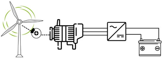
Figure 1. Wind energy system.

The figure shows the overall scheme of the conversion chain and the most important energy flows between the turbine, permanent magnet synchronous generator (PMSG), rectifier, and battery. This is a deliberately simplified model that brings out the essential functional relationships of the components without showing the internal equations, so a general understanding may be gained before the analytical and average models that will be discussed in the following sections are presented.

3.1. Generator Sizing

This study uses the generator model developed from the analytical formulation in the work of Tounsi [13], adapted for efficient integration within a multi-objective optimization framework. This choice is consistent with our recent work in [14,15] and approaches that have been validated by Gao et al. [16] and Zhang et al. [17], who have demonstrated the relevance of analytical models dealing with direct-drive PMSGs and sensorless control strategies.

The method followed in this analysis relies on the basic laws of electromagnetism like Ampère’s law, conservation of flux, and superposition of the field for the estimation of air-gap flux, induced electromotive force, and electromagnetic torque from geometric and material parameters. Validation by the finite element method (2-D EMF) presents very good agreement in the EMF amplitude, confirming the reliability and accuracy of the model for optimization studies. Figure 2 illustrates the geometric dimensions extracted from the analytical model, which have been used to make calculations of flux and EMF in the permanent magnet synchronous generator.

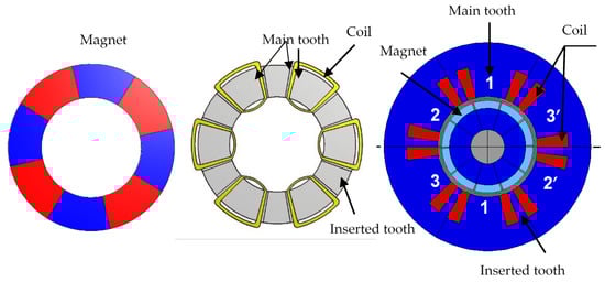
Figure 2. Dimension of generator.

The generator constant is mathematically represented as follows [14]:

$$K_e = 2 \times N_s \times F_A \times { F}_B \times B_g$$

(1)

For the axial flux structures F_A and F_B, the definitions are as follows [14]:

$$F_A ={\displaystyle \frac{D_{ex} - D_{in}}{2}}$$

(2)

$$F_B= {\displaystyle \frac{D_{ex}+{ D}_{in}}{2}}$$

(3)

where D_ex and D_in denote the generator’s external and internal diameters, respectively.

The torque used for dimensioning is defined by the following equation [14]:

$$T_{dim }= {\displaystyle \frac{1}{2}}\times {\displaystyle \frac{C_p\times R_p^2\times V_{wmax}^3}{{\Omega }_{max}}}$$

(4)

where V_wmax is the maximum airflow speed, R_p denotes the radius of the turbine blades, C_p denotes the power coefficient and Ω_max is the generator’s peak angular speed.

The sizing current can be calculated using the equation below [14]:

$$I_{dim}={\displaystyle \frac{T_{dim}}{2\times N_s\times A\times B\times B_g}}$$

(5)

The air-gap flux density is determined for the position where maximum recovery occurs, when the magnet is aligned with a main tooth. At this alignment, the air-gap flux density reaches its peak. Figure 3 illustrates the distribution of the field lines within a pole.

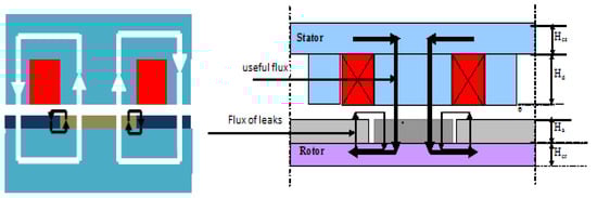
Figure 3. Flux line distribution at the peak recovery position.

Figure 3 illustrates the division of the flux into useful and leakage components between the magnets. The use of Ampere’s law results in Equation (6) [13]:

$$\int \underset{H}{\to }\times \underset{dl}{\to }={\displaystyle \frac{N_s}{\frac{N_d}{3}}}\times I_{max}=2\times \left(H_{ri}\times t_m+H_{ri}\times g\right)$$

(6)

where I_max is the maximum generator’s current, H denotes the magnetic field intensity, H_ri denotes the magnetic field across the air-gap, $t_m$ is the thickness of the permanent magnet, g is the gap thickness, μ₀ is the permeability of air, N_s defines the number of turns per phase and N_d the main teeth number [13].

$$B_{ri}={ H}_{ri}\times {\mu }_0$$

(7)

where B_ri is the air-gap flux density produced by current of stator [13].

$$B_{ri}={\displaystyle \frac{{\mu }_0}{2\times \frac{N_d}{3}}}\times {\displaystyle \frac{N_s\times I_{max}}{t_m+g}}$$

(8)

The application of the Ampere theorem, without consideration of the stator current, leads to Equation (9) [13]:

$$\int \underset{H}{\to }\times \underset{dl}{\to }=0=2\times \left(H_m\times t_m+H_g\times g\right)$$

(9)

Equation (10) defines the magnetic flux density in the air gap [15]:

$$B_g={\mu }_0\times H_g$$

(10)

Applying of the flux conservation theorem leads to Equation (11) [15]:

$$B_m\times S_m\times K_{fu}=B_g\times S_m$$

(11)

The magnet flux density is deduced from Equation (12) [15]:

$$B_m={\displaystyle \frac{B_g}{K_{fu}}}$$

(12)

Equation (13) defines the magnetic flux density [15]:

$$B_m={\mu }_0{\times \mu }_m\times H_m{+B}_r$$

(13)

where µ_m is the magnet’s relative permeability and B_r is the remanence.

Based on Equations (10)–(13), the magnet thickness is determined by defining the flux density in the air gap as B_g [13]:

$$T_m = {\mu }_m\times {\displaystyle \frac{B_g}{B_r-\frac{B_g}{K_{fu}}}} \times g_a$$

(14)

where K_fu (<1) represents the leakage parameter of the magnet, and g_a is the air-gap thickness. Phase currents must be kept under the demagnetization current I_d to prevent demagnetization [13].

$$I_d=\left({\displaystyle \frac{B_r-B_{min}}{{\mu }_m}}\times t_m-B_{min}\times K_{fu}\times g\right)\times {\displaystyle \frac{p}{2\times {{\mu }_0\times N}_s}}$$

(15)

where B_min is the magnet’s minimum flux density. The thicknesses of the rotor yoke (t_ry) and stator yoke (t_sy) are given by Equations (16) and (17) [14]:

$$T_{ry}={\displaystyle \frac{B_g}{B_{ry}}}\times {\displaystyle \frac{Min(A_t,{ A}_m)}{2\times A}}\times {\displaystyle \frac{I}{K_{fu}}}$$

(16)

$$T_{sy}={\displaystyle \frac{B_g}{B_{sy}}}\times {\displaystyle \frac{Min(A_t, A_m)}{2\times A}}$$

(17)

where A_t and A_m are the tooth and magnet areas, B_ry and B_sy correspond to the flux densities in the rotor and stator yokes.

The stator’s slot height is calculated from Equation (18) [15]:

$$h_s={\displaystyle \frac{3N_s}{N_t}}\times {\displaystyle \frac{1}{K_f \times A_s}}\times {\displaystyle \frac{I_{dim}}{\delta }}$$

(18)

wherein N_t represents the count of the main teeth, K_f indicates the slot fill ratio, As indicates the slot’s width, I_dim is the current used for dimensioning and δ is the current density in the slots [13].

$$I_{dim}={\displaystyle \frac{T_{dim}}{K_e}}$$

(19)

The width of the slot is calculated according to relation (20) [15]:

$$A_s= F_B\times sin\left({\displaystyle \frac{1}{2}}\times \left({\displaystyle \frac{2\pi }{N_t}}-\alpha \times \beta \times {\displaystyle \frac{\pi }{p}}\times \left(1-r_{did}\right)\right)\right)$$

(20)

Here, r_did is defined as the proportion of the angular width of the inserted tooth relative to the principal tooth; α represents the ratio between the angular widths of a main tooth and a magnet; β indicates the ratio of the magnet’s angular width to the pole pitch; and p stands for the number of pole pairs.

3.2. Optimization Process of Turbine Parameters

The developed algorithm for solving the optimal design problem of wind turbine parameters is described in Figure 4.

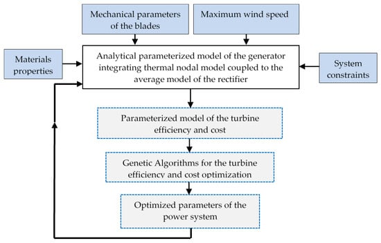
Figure 4. Algorithm for solving the optimal design problem of wind parameters.

For the effective optimization of an energy conversion system, ensuring a thorough understanding of every component, from the energy source to the point of use, is essential. In this study, we adopt a wind power conversion chain composed of an axial-flux permanent magnet synchronous generator connected with a diode rectifier, which stores the recovered power in batteries. A booster chop-per can be added to regulate the battery charging current. Also, a mechanical brake can be added to protect the turbine. To test the critical operating regime of the turbine (Maximum power generation depending on wind speed), only the mechanical part including the blades and the geared speed multiplier, the generator and the battery are considered for this study.

3.3. Turbine Model

The following equations define the induced electromotive forces e_a, e_b, and e_c [13] as follows:

$$e_a={\displaystyle \frac{2}{3}}{K}_e\times {\Omega }_g\times cos\left(p\times \Omega \times t+{\displaystyle \frac{\pi }{2}}\right)$$

(21)

$$e_b={\displaystyle \frac{2}{3}}{K}_e\times {\Omega }_g\times cos\left(p\times \Omega \times t+({\displaystyle \frac{\pi }{2}}-{\displaystyle \frac{2\pi }{3}})\right)$$

(22)

$$e_c={\displaystyle \frac{2}{3}}{K}_e\times { \Omega }_g\times cos\left(p\times \Omega \times t+({\displaystyle \frac{\pi }{2}}-{\displaystyle \frac{4\pi }{3}})\right)$$

(23)

where K_e denotes the electrical constant, Ωg denotes the angular speed and p is pole pairs pole number.

Each phase of the generator can be modeled as a resistor in series with an inductance and an induced electromotive force. The three-phase model of the generator is then described by the following equations:

$$e_a={ v}_a+(L-M)\times {\displaystyle \frac{{di}_a}{dt}} + R\times i_a$$

(24)

$$e_b=v_b+\left(L-M\right)\times {\displaystyle \frac{{di}_b}{dt}}+R\times i_b$$

(25)

$$e_c=v_c+(L-M)\times {\displaystyle \frac{{di}_c}{dt}}+R\times i_c$$

(26)

The parameters R, L, and M correspond to the resistance, inductance, and mutual inductance of phases a, b, and c, respectively. Meanwhile, i_a,b,c, e_a,b,c and v_a,b,c denote the currents, induced electromotive forces, and voltages for each of these phases.

The overall power chain configuration—including the generator, rectifier, and battery—is depicted in Figure 5.

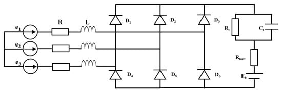
Figure 5. Generator-Rectifier-Battery model.

The motion equation for the rotating parts is obtained from the basic dynamic relationship [13,14,15].

$$J \times \frac{d\Omega }{dt}=T_m-r_d\times \left(T_{em}+T_{mec}+T_f\right)$$

(27)

where J represents the moment of inertia of the rotating components, r_d stands for the speed amplification ratio, and Ω indicates the angular velocity of the turbine. T_m refers to the torque generated by the wind acting on the motor shaft, T_em is the torque produced electromagnetically, T_mec corresponds to torque losses arising from mechanical friction, and T_f represents torque losses associated with iron components.

The various torques are represented by equations below:

$$T_m={\displaystyle \frac{1}{2}}\times {\displaystyle \frac{C_p\times R_p^2\times V_{wind}^3}{\Omega }}$$

(28)

where Cp is the turbine power coefficient, R_p is the radius blade, and V_wind is the speed.

$$T_{em}={\displaystyle \frac{1}{\Omega }}{\sum }_{i=1}^3{e}_i\times i_i$$

(29)

where e_i denotes the back electromotive force and i_i corresponds to the current in phase i.

$$T_{mec}=s+\Omega \times \left(K+\gamma \times \Omega \right)$$

(30)

where the parameters s, K, and g correspond to the dry, viscous, and fluid friction coefficients, respectively, and V indicates the angular velocity of the generator.

Figure 6 is an illustration of the globally wind energy system model.

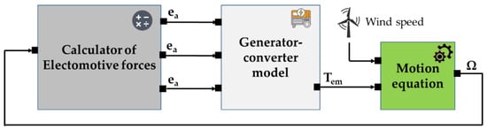
Figure 6. Global structure of wind energy system.

4. Average Models of Wind Energy System

The systems design approach requires the development of mean-value models for each major component. These models are detailed here because they provide the necessary balance between the physical consistency needed at the sizing stage and computational efficiency necessary for the thorough study of the system.

4.1. First Wind Energy System Average Model

Figure 7 displays the corresponding schematic for the generator-inverter-battery arrangement.

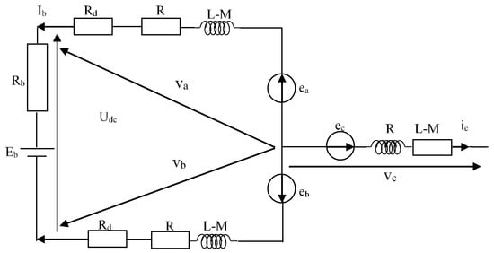
Figure 7. Equivalent model of generator-inverter-battery.

Figure 8 presents the vector diagram corresponding to a battery load, modeled as an internal voltage source in series with its internal resistance.

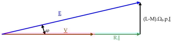
Figure 8. Vector diagram.

V, E, and I refer, respectively, to the phase voltage, electromotive force, and current vectors, while L and M denote the phase’s self and mutual inductances.

Equation (31) is deduced from vector diagram (Figure 8).

$${E^2=\left(V+RI\right)}^2{+\left({\Omega }_g\times p\times I\times \left(L-M\right)\right)}^2$$

(31)

By rearranging Equation (31), we obtain Equation (32).

$$V=\sqrt{E^2-{\left({\Omega }_g\times p\times I\times \left(L-M\right)\right)}^2} - RI$$

(32)

The mean value of the phase 1–2 voltage (u12) is given by Equation (33).

$$u_a={\displaystyle \frac{1}{T}}{\int }_0^T{u}_{12}\times dt=\sqrt{3}\times {\displaystyle \frac{3}{\pi }}\times V$$

(33)

The DC bus voltage (U_dc), which charges the battery, can be determined by utilizing the results from Equations (32) and (33).

$$U_{dc}=\left(\sqrt{E^2-{\left({\Omega }_g\times p\times I\times \left(L-M\right)\right)}^2}- \left(R-R_d\right)I\right)\times \sqrt{3}\times {\displaystyle \frac{3}{\pi }}+2V_d$$

(34)

where V_d corresponds to the voltage drop across the diodes and R_d denotes their internal resistance.

The magnitude of the current in the generator phase can be defined using Relation (35).

$$I={\displaystyle \frac{3 I_b}{\pi }}$$

(35)

where I_b denotes the current used to recharge the battery

By combining Equations (34) and (35), Relation (36) is obtained.

$$U_{dc}=\left(\sqrt{E^2-{\left(\left(L-M\right)\times {\Omega }_g\times p\times I_b\times {\displaystyle \frac{\pi }{3}}\right)}^2}-\left(R-R_d\right){\displaystyle \frac{\pi }{3}}\times I_b\right)\times \sqrt{3}\times {\displaystyle \frac{3}{\pi }}+2V_d$$

(36)

Equation (37) provides the expression for the electromotive force magnitude.

$$E={\displaystyle \frac{2}{3}}{K}_e\times {\Omega }_g$$

(37)

The Relation (38) is derived from Equations (36) and (37).

$$U_{dc}=\left(\sqrt{{\left({\displaystyle \frac{2}{3}}{K}_e\times {\Omega }_g\right)}^2-{\left({\Omega }_g\times p\times I\times \left(L-M\right)\right)}^2}-\left(R-R_d\right){\displaystyle \frac{\pi }{3}}\times I_b\right)\times \sqrt{3}\times {\displaystyle \frac{3}{\pi }}+2V_d$$

(38)

$$I_b={\displaystyle \frac{U_{dc}-E_b}{R_b}}$$

(39)

where E_b stands for the internal voltage generated by the battery.

Equation (40) provides an estimate of the recovered energy (W_r).

$$W_r=\int E_b\times I_b\times dt$$

(40)

Equation (41) provides the estimation of the power factor.

$$\phi ={tan}^{-1}\left({\displaystyle \frac{ \frac{\pi }{ 3 } I_b\times L\times {\Omega }_g\times p}{\frac{\left(U_{dc}-2V_d\right)}{\frac{\pi }{3} \times \sqrt{3}}+\frac{\pi }{3} I_b\left(R+R_b\right) }}\right)$$

(41)

Equation (42) provides the expression for calculating the electromagnetic torque.

$$T_{em}=-K_e\times I_b\times {\displaystyle \frac{\pi }{3}} cos\left({tan}^{-1}\left({\displaystyle \frac{L\times {\Omega }_g\times p\times I_b\times \frac{\pi }{3}}{\frac{\left(U_{dc}-2V_d\right)}{\sqrt{3}\times \frac{\pi }{3}}+\left(R+R_b\right) I_b\times \frac{\pi }{3}}}\right)\right)$$

(42)

Figure 9 illustrates the global power system average model.

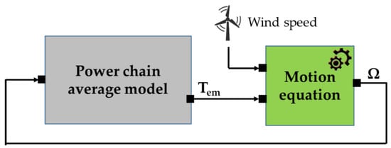
Figure 9. First Average Model for the Wind Energy Conversion System.

4.2. Second Wind Energy System Average Model

Figure 10 shows the equivalent schematic of the power system, including the generator, inverter, and battery.

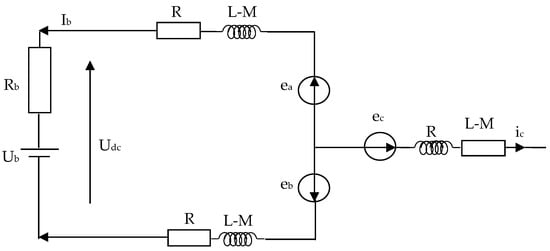
Figure 10. Second Wind Energy System Average Model.

The phases of the generator’s currents are illustrated in Figure 11.

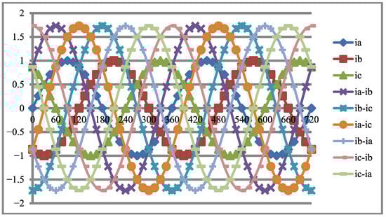
Figure 11. Paces of the currents.

According to Figure 7, the following relation expresses the average battery recharging voltage.

$$U_{dc}={\displaystyle \frac{1}{\frac{\pi }{3}}}{\int }_{{\displaystyle \frac{\pi }{3}}}^{{\displaystyle \frac{2\pi }{3}}}\left(e_a-e_b-R\left(i_a-i_b\right)-\left(L-M\right)\times \left({\displaystyle \frac{{di}_a}{dt}}-{\displaystyle \frac{{di}_b}{dt}}\right)\right)d\theta$$

(43)

Equation (44) can be transformed to Equation (46).

$$U_{dc}={\displaystyle \frac{1}{\frac{\pi }{6}}}{\int }_{{\displaystyle \frac{\pi }{6}}}^{{\displaystyle \frac{2\pi }{6}}}\left(e_{ab}-R\left(i_a-i_b\right)-\left(L-M\right)\times \left({\displaystyle \frac{d\left(i_a-i_b\right)}{dt}}\right)\right)d\theta$$

(44)

The generator’s phase of currents i_a and i_b are expressed by Relations (45) and (46).

$$I_a=I_s\times sin\left(\omega \times t-\phi \right)$$

(45)

$$I_b=I_s\times sin\left(\omega \times t-{\displaystyle \frac{2\pi }{3}}-\phi \right)$$

(46)

The difference between the currents i_a and i_b can be expressed by Relation (47).

$$I_a-I_b=I_s\left(sin(\omega \times t-\phi )-sin\left(\omega \times t-{\displaystyle \frac{2\pi }{3}}-\phi \right)\right)$$

(47)

Relation (47) can be transformed into Relation (48).

$$I_a{-I}_b=\sqrt{2}{\times I}_s\times sin\left(\omega \times t+{\displaystyle \frac{\pi }{6}}-\phi \right)$$

(48)

Considering Equation (48).

$$I_s={\displaystyle \frac{\pi }{3}}\times I_b$$

(49)

The difference between currents a_i and i_b is given by the following Equation (50).

$${\displaystyle \frac{\omega }{\frac{\pi }{6}}}{\int }_{{\displaystyle \frac{\pi }{6\omega }}+{\displaystyle \frac{\phi }{\omega }}}^{{\displaystyle \frac{2\pi }{6\omega }}+{\displaystyle \frac{\phi }{\omega }}}\left(i_a-i_b\right)dt=\sqrt{3}\times I_s\times {\displaystyle \frac{3}{\pi }}=\sqrt{3}\times {\displaystyle \frac{3}{\pi }}\times I_b$$

(50)

The mean derivative of the current difference (i_a − i_b) can be obtained from Equation (51):

$${\displaystyle \frac{\omega }{\frac{\pi }{6}}}{\int }_{{\displaystyle \frac{\pi }{6\omega }}+{\displaystyle \frac{\phi }{\omega }}}^{{\displaystyle \frac{2\pi }{6\omega }}+{\displaystyle \frac{\phi }{\omega }}}{\displaystyle \frac{d}{dt}}\left(i_a-i_b\right)dt=I_b\times {\displaystyle \frac{\omega }{\frac{\pi }{6}}}{\left[i_a-i_b\right]}_{{\displaystyle \frac{\pi }{6\omega }}}^{{\displaystyle \frac{2\pi }{6\omega }}}={\displaystyle \frac{6}{\pi }}\times \omega \times I_b\times {\displaystyle \frac{1}{2}}\times \sqrt{3}={\displaystyle \frac{3}{\pi }}\times \sqrt{3}\times \omega \times I_b$$

(51)

As with the currents, the average value of the difference in induced electromotive forces e_a and e_b (Equation (52)) is derived from Relations (53) to (58):

$$e_a={\displaystyle \frac{2}{3}}\times K_e\times {\displaystyle \frac{\omega }{p}}\times cos\left(\omega \times t-{\displaystyle \frac{\pi }{2}}\right)$$

(52)

$$e_b={\displaystyle \frac{2}{3}}\times K_e\times {\displaystyle \frac{\omega }{p}}\times cos\left(\omega \times t-{\displaystyle \frac{2\pi }{3}}-{\displaystyle \frac{\pi }{2}}\right)$$

(53)

$$e_a-{ e}_b={\displaystyle \frac{2}{3}}\times K_e\times {\displaystyle \frac{\omega }{p}}\times \left(cos\left(\omega \times t-{\displaystyle \frac{\pi }{2}}\right)-cos\left(\omega \times t-{\displaystyle \frac{2\pi }{3}}-{\displaystyle \frac{\pi }{2}}\right)\right)$$

(54)

$$e_a-{ e}_b=\sqrt{3}\times {\displaystyle \frac{2}{3}}\times K_e\times {\displaystyle \frac{\omega }{p}}\times cos\left(\omega \times t+{\displaystyle \frac{\pi }{2}}+{\displaystyle \frac{\pi }{6}}\right)$$

(55)

$$e_{ab}=e_a-{ e}_b=-\sqrt{3}\times {\displaystyle \frac{2}{3}}\times K_e\times {\displaystyle \frac{\omega }{p}}\times sin\left(\omega \times t+{\displaystyle \frac{\pi }{6}}\right)$$

(56)

$$e_{ab}=e_a-e_b=\sqrt{3}\times {\displaystyle \frac{2}{3}}\times K_e\times {\displaystyle \frac{\omega }{p}}\times sin\left(\omega \times t+{\displaystyle \frac{\pi }{6}}+\pi \right)$$

(57)

$${\displaystyle \frac{\omega }{\frac{\pi }{6}}}\times {\int }_{{\displaystyle \frac{\pi }{6\omega }}+{\displaystyle \frac{\pi }{6\omega }}}^{{\displaystyle \frac{2\pi }{6\omega }}+{\displaystyle \frac{\pi }{6\omega }}}{e}_{ab}dt={\displaystyle \frac{\omega }{\frac{\pi }{6}}} {\left[e_{ab}\right]}_{{\displaystyle \frac{\pi }{6\omega }}-{\displaystyle \frac{\pi }{6\omega }}+{\displaystyle \frac{\pi }{\omega }}}^{{\displaystyle \frac{2\pi }{6\omega }}-{\displaystyle \frac{\pi }{6\omega }}+{\displaystyle \frac{\pi }{\omega }}}={\displaystyle \frac{6}{\pi }}\times {\displaystyle \frac{1}{2}}\times \sqrt{3}\times {\displaystyle \frac{2}{3}}\times K_e\times {\displaystyle \frac{\omega }{p}}={\displaystyle \frac{\pi }{3}}\times \sqrt{3}\times {\displaystyle \frac{2}{3}}\times K_e\times {\displaystyle \frac{\omega }{\pi }}$$

(58)

Equations (59) and (60) define the average value of the battery recharging voltage:

$$U_{dc}={\int }_{{\displaystyle \frac{\pi }{6\omega }}+{\displaystyle \frac{\pi }{6\omega }}}^{{\displaystyle \frac{2\pi }{6\omega }}+{\displaystyle \frac{\pi }{6\omega }}}{e}_{ab}dt-R\times {\displaystyle \frac{\omega }{\frac{\pi }{6}}}\times {\int }_{{\displaystyle \frac{\pi }{6\omega }}+{\displaystyle \frac{\phi }{\omega }}}^{{\displaystyle \frac{2\pi }{6\omega }}+{\displaystyle \frac{\phi }{\omega }}}\left(i_a-i_b\right)dt-(L-M)\times {\displaystyle \frac{\omega }{\frac{\pi }{6}}}\times {\int }_{{\displaystyle \frac{\pi }{6\omega }}+{\displaystyle \frac{\phi }{\omega }}}^{{\displaystyle \frac{2\pi }{6\omega }}+{\displaystyle \frac{\phi }{\omega }}}{\displaystyle \frac{d}{dt}}\left(i_a-i_b\right)dt$$

(59)

$$U_{dc}={\displaystyle \frac{3}{\pi }}\times \sqrt{3}\times {\displaystyle \frac{2}{3}}\times K_e\times {\displaystyle \frac{\omega }{p}}-R\times {\displaystyle \frac{3}{\pi }}\times \sqrt{3}\times I_b-\left(L-M\right)\times {\displaystyle \frac{3}{\pi }}\times \sqrt{3}\times \omega \times I_b$$

(60)

Equation (61) can be simplified into Equation (62).

$$U_{dc}=E_{dc}-R_{dc1}\times I_b-R_{dc2}\times I_b=E_{dc}-\left(R_{dc1}+R_{dc2}\left(\omega \right)\right)\times I_b$$

(61)

where

$$E_{dc}={\displaystyle \frac{3}{\pi }}\times \sqrt{3}\times {\displaystyle \frac{2}{3}}\times K_e\times {\displaystyle \frac{\omega }{p}}$$

(62)

$$R_{dc1}=R\times \sqrt{3}\times {\displaystyle \frac{3}{\pi }}$$

(63)

$$\omega =p\times \Omega$$

(64)

The electromagnetic torque can be expressed by Relation (65).

$$T_{em}=K_e\times I_b\times cos\left(\phi \right)$$

(65)

Using the vector diagram, the phase shift φ is calculated.

$$\phi ={tan}^{-1}\left({\displaystyle \frac{\left(L-M\right)\times p\times \Omega \times I_p}{\left(\frac{U_{dc}}{\sqrt{3}}\times \frac{\pi }{3}\right)+\left(R+R_d\right)\times I_b}}\right)$$

(66)

Figure 12 depicts the implementation of the wind turbine’s DC model within Matlab-Simulink.

Figure 12. Wind turbine DC model.

It should be mentioned that the mean-value model adopted for modeling the power converter is an intentional simplification with respect to the detailed switching models available in MATLAB/Simulink. Indeed, the AVM eliminates the high-frequency effects associated with the switching actions and retains only the average quantities (DC voltage, power, average currents) relevant for energy analysis and optimization. This simplification may result in a slight loss of accuracy with respect to the current ripple and instantaneous harmonics; however, it preserves the electromagnetic and energy quantities used in the sizing and optimization steps with good fidelity [4,5]. The comparative validation performed with the detailed Simulink model shows satisfactory agreement on the average variables that fully justifies the use of the average analytical model in a systemic optimization framework where computational speed and physical consistency are essential.

5. Simulation Results

The parameters presented in Table 1 were adopted to ensure the physical consistency and practical applicability of the simulations. These values are not arbitrary; they are derived from the technical specifications of a real, low-power wind turbine system, which serves as a reference for the sizing and validation of the model. Their use in the average models ensures a realistic and reproducible simulation framework, enhancing the reliability of the optimization results obtained. According to the data provided by the analytical model of the wind turbine, simulations of the power chain model were conducted for all three cases.

Table 1. Simulation parameters.

Parameters	Values	Units
Nominal battery voltage (Udc)	100	Volts
Internal resistance of the battery (Rb).	0.2	Ω
Diodes internal resistance (Rd)	0.001	Ω
Generator electric constant (Ke).	24	Volt/(rad/s)
Electrical resistance (R).	1	Ω
Equivalent inductance (L).	0.00014123	H
Mutual inductance (M).	0.00004121	H
Gear ratio (rd).	2	/

The evolution of wind speed over time is illustrated in Figure 13. This behavior reveals periods of high acceleration and overspeed, important factors for respecting turbine speed constraints and properly sizing the power chain current.

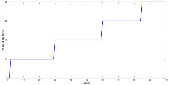
Figure 13. Speed of the wind.

Figure 14 displays how the power factor varies over time for each of the three model configurations. The close alignment of the results across all cases serves as strong confirmation of the study’s validity.

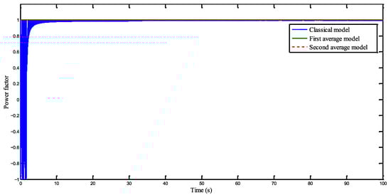
Figure 14. Variation in the power factor over time.

Figure 15 presents the time evolution of the electromagnetic torque for the three model cases. The close agreement between the results confirms the validity of the developed study.

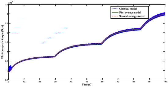
Figure 15. Electromagnetic torque.

Figure 16 illustrates the time evolution of the battery recharging voltage for the three model cases. It also highlights the close similarity among the three results, which confirms the validity of the developed study.

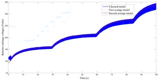
Figure 16. Variation in the battery’s charging voltage.

Figure 17 shows the temporal variation in recovered energy across the three model scenarios. The close correspondence among the results further confirms the validity of the developed study.

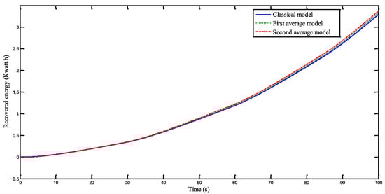
Figure 17. Recovered energy.

In order to strengthen the credibility of the proposed model, a deep comparative study has been carried out between the average analytical model and the detailed switching model available in MATLAB/Simulink. As can be seen from the results, although no explicit switching is present in the averaged model, the key energy values such as average rectified voltage, input current, ripple factor, and electromagnetic power deviate very slightly from the detailed model while systematically agreeing on the mid-scale dynamic behavior. These observations follow the conclusions available in the literature, where it was shown that average models faithfully reproduce quantities of interest in energy optimization and control studies [4,5,8]. Moreover, the use of the average analytical model reduces the computation time drastically and allows this model to be used within a stochastic optimization loop, something impossible with the detailed model due to its heavy computational cost. As shown by the consistency between experimental and simulated curves, the averaged model constitutes a sufficiently faithful representation for systemic design while bringing the speed indispensable to the optimization algorithms used in this study.

6. Optimization of the Turbine Power System Recovered Energy

In this work, a GA is preferred for the optimization because it is not only robust and adaptive but also extensively used in solving nonlinear and multi-objective problems characteristic of wind energy conversion systems. Unlike other classical deterministic methods, the GA does not require the differentiability or convexity of the objective function. This makes it specially adapted to optimization problems involving complex interactions between the aerodynamic, electromagnetic, and thermal phenomena of the conversion chain.

Several recent studies have demonstrated the superiority of the genetic algorithm in the optimization of energy systems, especially regarding multi-parameter tuning and constrained design. As an example, Hemeida et al. [18] proved the efficiency of the GA in the search for the maximum power point in synchronous generator wind power systems, while the robustness against local minima and modeling uncertainties has been confirmed by Benbouhenni et al. [11], Fathy et al. [12], and Poudel et al. [9] compared with other algorithms such as PSO or ACO.

In that respect, the genetic algorithm was adopted as the basis for the proposed optimization methodology, given its effectiveness, ease of combination with analytical and other models, and global searching capability, which would provide an optimal compromise between accuracy, computational cost, and practical feasibility. This choice ensures reliable and rapid optimization of the electromechanical and energy parameters of the studied wind power conversion system.

6.1. Optimization Problem Resolution

The developed approach (refer to Figure 18) combines the analytical design model, the average model, and an improved genetic algorithm. Enhancements to the genetic algorithm consist of retaining the best N individuals from generation i for reproduction in generation i + 1, alongside a stopping criterion based on the convergence of the precision function—specifically, the simulation terminates when the difference in precision between consecutive iterations satisfies: Prec[i + 1] − Prec[i] = 0 [18,19,20,21,22,23].

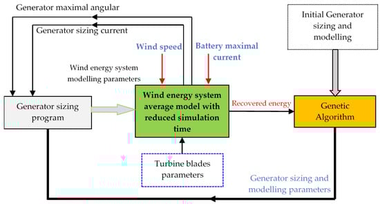
Figure 18. Architectural scheme of the software optimization program.

After the analysis of the optimization problem, we find that the optimization of the energy recovery system depends on all the parameters mentioned in Equation (67). The optimization problem is summarized as follows:

$$\left\{\begin{array}{c}Maximize \\ Prec\left(t\right)\\ Optimization parameters\\ 10\le { r}_d \le 20\\ 200\le { D}_e \le 400 \mathrm{mm}\\ 80\le { D}_i \le 180 \mathrm{mm}\\ 0.45\le { B}_g \le 1.4 \mathrm{Tesla}\\ 0.2\le \delta \le 7 \mathrm{A}/{\mathrm{mm}}^2\\ 0.2\le { B}_{cs} \le 1.6 \mathrm{Tesla}\\ 0.2\le { B}_{cr} \le 1.6 \mathrm{Tesla}\\ 1\le { N}_s \le 30 \\ constraints\\ \left(L-M\right)\times {\displaystyle \frac{di}{dt}}\le 2 volt\\ M_{g } \le 200 \mathrm{kg}\end{array}\right\}$$

(67)

where L and M denote the inductance and mutual inductance of the generator, respectively, and M_g represents the generator’s mass.

6.2. Simulation Results After Optimization

To attain the maximum energy recovery from the developed wind system models, we conduct multiple trials with varying instruction counts ranging from 100 to 600.

6.2.1. Solution for 100 Iterations

Table 2 presents the optimal solution obtained after 100 iterations with a population size of 200.

Table 2. Optimal solution for 200 populations.

Parameters	Iterations	Rd	Dext (mm)	Dint (mm)	Be (Tesla)	δ (A/mm2)	Bcs (Tesla)	Bcr (Tesla)	Nsph	Prec (kw)
Values	100	15.5	359.5	116.4	0.676	2.66	0.54	1.58	20	74.5167

Figure 19 illustrates the evolution the objective function for 100 iterations. The simulation takes approximately 1 day. Figure 19 demonstrates that the optimal solution is not achieved.

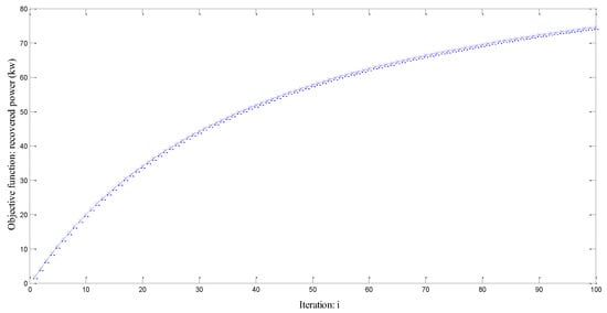
Figure 19. Objective function: recovered power (kw) for 100 iterations.

6.2.2. Solution for 200 Iterations

Table 3 presents the optimal solution obtained after 200 iterations with a population size of 400.

Table 3. Optimal solution for 400 populations.

Parameters	Iterations	rd	Dext (mm)	Dint (mm)	Be (Tesla)	δ (A/mm2)	Bcs (Tesla)	Bcr (Tesla)	Nsph	Prec (kw)
Values	200	13	263	90.4	0.69	6.8	1.43	0.85	29	87.261

Figure 20 illustrates the evolution of objective function for 200 iterations. The simulation time is approximately 2.5 days. It illustrates that the optimal solution is not achieved.

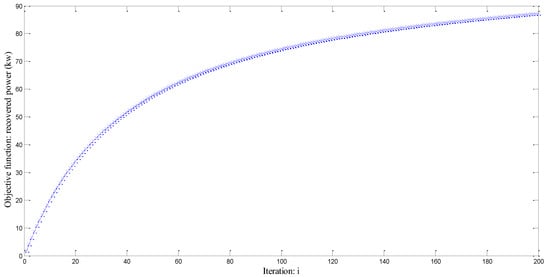
Figure 20. Objective function: recovered power (kw) for 200 iterations.

6.2.3. Solution for 300 Iterations

Table 4 presents the optimal solution obtained after 300 iterations with a population size of 400.

Table 4. Optimal solution for 400 populations (300 iterations).

Parameters	Iterations	rd	Dext (mm)	Dint (mm)	Be (Tesla)	δ (A/mm2)	Bcs (Tesla)	Bcr (Tesla)	Nsph	Prec (kw)
Values	300	16.5	297	177	0.6726	2.1	1.37	0.99	22	86.7218

Figure 21 illustrates the evolution of the objective function for 300 iterations. Simulation takes 3 day approximately. Figure 21 illustrates that the optimal solution is improved but not achieved.

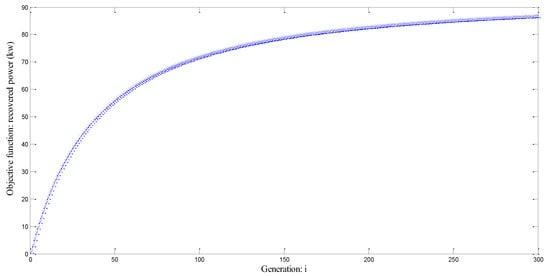
Figure 21. Objective function: recovered power (kw) for 300 iterations.

6.2.4. Solution for 400 Iterations

Table 5 presents the optimal solution obtained after 400 iterations with a population size of 400.

Table 5. Optimal solution for 400 populations (400 iterations).

Parameters	Iterations	rd	Dext (mm)	Dint (mm)	Be (Tesla)	δ (A/mm2)	Bcs (Tesla)	Bcr (Tesla)	Nsph	Prec (kw)
Values	400	11	354	153.6	0.6	3.13	1.25	0.67	4	88.6769

Figure 22 illustrates the objective function for 300 iterations. Figure 22 demonstrates the beginning of convergence towards the optimal solution.

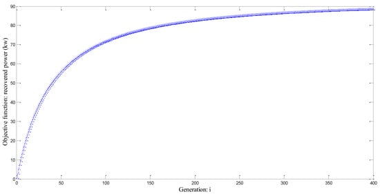
Figure 22. Objective function: recovered power (kw) for 400 iterations.

6.2.5. Solution for 500 Iterations

Table 6 presents the optimal solution obtained after 500 iterations with a population size of 400.

Table 6. Optimal solution for 400 populations (500 iterations).

Parameters	Iterations	rd	Dext (mm)	Dint (mm)	Be (Tesla)	δ (A/mm2)	Bcs (Tesla)	Bcr (Tesla)	Nsph	Prec (kw)
Values	500	14	343	159.67	0.54	5.1	1.05	1.109	20	89.816

Figure 23 illustrates the evolution of the objective function for 500 iterations. Figure 23 illustrates that the optimal solution is achieved (The derivative the objective function is equal to 0).

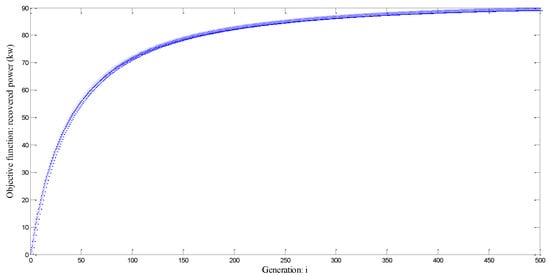
Figure 23. Objective function: recovered power (kw) for 500 iterations.

6.2.6. Optimal Value of the Recovered Power (kw) in Function Total Generations Number

Figure 24 illustrates the optimal value of the recovered power (kw) in function of the total number of generations. Figure 24 demonstrates that the augmentation of the number of generation improve significantly the optimal solution.

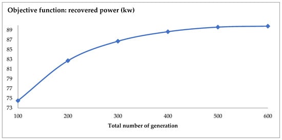
Figure 24. Variation in the optimized recovered power over successive generations.

Increasing the population size significantly improves the objective function. Finding the iterations number needed to find the optimal solution is difficult and time-consuming, and subsequently the optimal solution is poorly controllable by varying the number of iterations. In this case, the study cost increases enormously. The derivation of the objective function leads directly to the optimal solution, which is subsequently chosen as the stopping criterion.

7. Conclusions

This paper introduces a systemic design methodology based on the novel coupling of a rigorous analytical model of the PMSG with an average-value model of the power converter for a wind turbine’s conversion chain. This combination is the major innovative element of this study: it gives a unified, fast, and physically consistent model that can advantageously replace detailed models whose computation times are incompatible with iterative optimization processes. The two models were validated by comparing them against reference MATLAB/Simulink models. This validation confirms the accuracy and physical consistency of the proposed framework while significantly reducing the computational cost. Afterward, this coupled model was inserted within an improved genetic algorithm in order to optimize the recovered power under electrical, thermal, and dynamic constraints. Simulations show that the methodology allows us to obtain robust, reproducible, and effective results for designing modern wind power systems.

Beyond the results obtained, the fundamental contribution is to establish a generalizable methodological framework. This coupled model, combined with stochastic optimization, could be applied to other conversion architectures, including those with other kinds of generators like the DFIG. Finally, the approach developed here is directly transferable to experimental validation on a test bench or a microturbine. Its real-world implementation represents a natural step toward confirmation of the industrial and operational relevance of the methodology developed.

References

- Ligęza, P. Basic, Advanced, and Sophisticated Approaches to the Current and Forecast Challenges of Wind Energy. Energies 2021, 14, 8147. [Google Scholar] [CrossRef]
- Li, W. Design and kinetic analysis of wind turbine blade-hub-tower coupled system. Renew. Energy 2016, 94, 547–557. [Google Scholar] [CrossRef]
- Asim, T.; Islam, S.Z.; Hemmati, A.; Khalid, M.S.U. A Review of Recent Advancements in Offshore Wind Turbine Technology. Energies 2022, 15, 579. [Google Scholar] [CrossRef]
- Rajendran, S.; Díaz, M.; Cárdenas, R.; Espina, E.; Contreras, E.; Rodriguez, J. A Review of Generators and Power Converters for Multi-MW Wind Energy Conversion Systems. Processes 2022, 10, 2302. [Google Scholar] [CrossRef]
- He, X.; Geng, H.; Mu, G. Modeling of wind turbine generators for power system stability studies: A review. Renew. Sustain. Energy Rev. 2021, 143, 110865. [Google Scholar] [CrossRef]
- Cultura, A.B.; Salameh, Z.M. Modeling and simulation of a wind turbine-generator system. In Proceedings of the IEEE Power and Energy Society General Meeting, Detroit, MI, USA, 24–28 July 2011; pp. 1–7. [Google Scholar] [CrossRef]
- Kasaeian, A.; Rahmani, K.; Fakoor, M.; Kosari, A.; Katooli, M.H. Systematic design of a wind turbine by Design Structure Matrix (DSM) method, case study: Lootak region. Int. J. Ambient. Energy 2024, 45, 2308041. [Google Scholar] [CrossRef]
- Guediri, A.; Hettiri, M.; Guediri, A. Modeling of a Wind Power System Using the Genetic Algorithm Based on a Doubly Fed Induction Generator for the Supply of Power to the Electrical Grid. Processes 2023, 11, 952. [Google Scholar] [CrossRef]
- Poudel, P.; Kumar, R.; Narain, V.; Jain, S.C. Power Optimization of a Wind Turbine Using Genetic Algorithm. In Machines, Mechanism and Robotics; Springer Nature: Berlin/Heidelberg, Germany, 2022; pp. 1943–1953. [Google Scholar] [CrossRef]
- Benbouhenni, H.; Gasmi, H.; Colak, I.; Bizon, N.; Thounthong, P. Synergetic-PI controller based on genetic algorithm for DPC-PWM strategy of a multi-rotor wind power system. Sci. Rep. 2023, 13, 13570. [Google Scholar] [CrossRef]
- Benbouhenni, H.; Bizon, N.; Yessef, M.; Elbarbary, Z.M.S.; Colak, I.; Bossoufi, B.; Al Ayidh, A. Experimental analysis of genetic algorithm-enhanced PI controller for power optimization in multi-rotor variable-speed wind turbine systems. Sci. Rep. 2025, 15, 1407. [Google Scholar] [CrossRef] [PubMed]
- Fathy, A.; Alharbi, A.G.; Alshammari, S.; Hasanien, H.M. Archimedes optimization algorithm based maximum power point tracker for wind energy generation system. Ain Shams Eng. J. 2022, 13, 101548. [Google Scholar] [CrossRef]
- Tounsi, S. Conversion of AC wind energy system model to DC model for integration to optimization software with large scales. Wind. Eng. (SAGE) 2021, 46, 240–259. [Google Scholar] [CrossRef]
- Hadj Abdallah, S.; Tounsi, S. Optimal design and control of AC–DC–DC wind energy system for electric vehicle batteries recharging stations. Int. J. Power Energy Syst. 2024, 44, 1–9. [Google Scholar] [CrossRef]
- Hadj Abdallah, H.A.; Tounsi, S. Optimal Control Structure of DC Current Generator with Concentrated Winding. In Proceedings of the 2024 4th International Conference on Innovative Research in Applied Science, Engineering and Technology (IRASET), Fez, Morocco, 16–17 May 2024; pp. 1–6. [Google Scholar] [CrossRef]
- Gao, L.; Hu, J.; Xu, L.; Zhu, Z.Q. Nonlinear maximum power extraction control of PMSG-based wind energy conversion systems: A review and new perspective. Renew. Sustain. Energy Rev. 2020, 133, 110296. [Google Scholar] [CrossRef]
- Shen, X.; Xie, T.; Wang, T.A. A Fuzzy Adaptative Backstepping Control Strategy for Marine Current Turbine under Disturbances and Uncertainties. Energies 2020, 13, 6550. [Google Scholar] [CrossRef]
- Hemeida, A.M.; El-Fergany, A.A.; Hasanien, H.M. Enhanced genetic algorithm-based optimal control for wind energy conversion systems considering maximum power point tracking. Energies 2020, 13, 3594. [Google Scholar] [CrossRef]
- Chhipą, A.A.; Chakrabarti, P.; Bolshev, V.; Chakrabarti, T.; Samarin, G.; Vasilyev, A.N.; Ghosh, S.; Kudryavtsev, A. Modeling and Control Strategy of Wind Energy Conversion System with Grid-Connected Doubly-Fed Induction Generator. Energies 2022, 15, 6694. [Google Scholar] [CrossRef]
- Abdallah, S.; Tounsi, S. Optimal Electric Vehicle Design Tool Using Genetic Algorithms. SAE Int. J. Passeng. Cars-Electron. Electr. Syst. 2018, 11, 109–122. [Google Scholar] [CrossRef]
- Fan, Z.; Zhu, C. The optimization and the application for the wind turbine power-wind speed curve. Renew. Energy 2019, 140, 52–61. [Google Scholar] [CrossRef]
- Abdelsalam, A.M.; El-Shorbagy, M. Optimization of wind turbines siting in a wind farm using genetic algorithm based local search. Renew. Energy 2018, 123, 748–755. [Google Scholar] [CrossRef]
- Guediri, M.; Ikhlef, N.; Bouchekhou, H.; Guediri, A.; Guediri, A. Optimization by Genetic Algorithm of a Wind Energy System applied to a Dual-feed Generator. Eng. Technol. Appl. Sci. Res. 2024, 14, 16890–16896. [Google Scholar] [CrossRef]
Disclaimer/Publisher’s Note: The statements, opinions and data contained in all publications are solely those of the individual author(s) and contributor(s) and not of MDPI and/or the editor(s). MDPI and/or the editor(s) disclaim responsibility for any injury to people or property resulting from any ideas, methods, instructions or products referred to in the content. |
© 2025 by the authors. Licensee MDPI, Basel, Switzerland. This article is an open access article distributed under the terms and conditions of the Creative Commons Attribution (CC BY) license (https://creativecommons.org/licenses/by/4.0/).