Routing Technologies for 6G Low-Power and Lossy Networks

Abstract

6G low-power and lossy network (6G LLN) is a kind of distributed network designed for IoT and edge computing scenarios of the sixth-generation mobile communication technology. Its routing technologies should fully consider characteristics of green and low carbon, constrained nodes, lossy links, etc. This paper proposes an improved routing protocol for low-power and lossy networks (I-RPL) to better suit the characteristics of 6G LLN and meet its application requirements. I-RPL has designed new context-aware routing metrics, which include the residual energy indicator, buffer utilization ratio, ETX, delay, and hop count to meet multi-dimensional network QoS requirements. The candidate parent and its preferred parent’s residual energy indicator and buffer utilization ratio are calculated recursively to reduce the effect of upstream parents. ETX and delay calculating methods are improved to ensure a better performance. Moreover, I-RPL has optimized the network construction process to improve energy and protocol efficiency. I-RPL has designed scientific multiple routing metrics evaluation theories (Lagrangian multiplier theories), proposed new rank computing and optimal route selecting mechanisms to simplify protocol, and optimized broadcast suppression and network reliability. Finally, theoretical analysis and experiment results show that the average end-to-end delay of I-RPL is 13% lower than that of RPL; the average alive node number increased 11% and so on. So, I-RPL can be applied well to the 6G LLN and is superior to RPL and its improvements.

1. Introduction

The 6G low-power and lossy network (6G LLN) [1,2] is a type of green and low-carbon network that enables intelligent interconnection and symbiotic coexistence among humans, machines, and things, contributing to the realization of the vision of “intelligent connection of all things and digital twins”. Due to its unstable links, limited bandwidth, and restricted processing capabilities of nodes, it is widely applied in smart city communications, disaster monitoring, smart grids, and national defense and the military, holding significant research and strategic value. The routing technology in 6G LLN is mainly responsible for the selection and forwarding of data transmission paths, which is crucial for ensuring efficient data transmission and network service quality. However, it faces numerous challenges in complex networking environments.

Therefore, this paper proposed an improved routing technology used for 6G LLN, which can better adapt to the characteristics of 6G LLN and ensure network QoS.

The main contributions presented in this paper are as follows:

(1)

An improved network topology construction process is proposed.

(2)

The new context-aware routing metrics, which include the residual energy indicator, buffer utilization ratio, ETX, delay, and hop, are proposed.

(3)

The recursive method is designed to calculate the candidate parent and its preferred parent’s residual energy indicator and buffer utilization ratio.

(4)

The ETX and delay calculating manner are improved.

(5)

Scientific multiple routing metric evaluation theories are designed.

(6)

A novel composite context-aware objective function (C-OF) is designed.

(7)

New rank computing and the optimal route selecting mechanisms are proposed.

The rest of this paper is organized in the following manner: Section 2 discusses the related works including the basic theory of 6G LLN and problems description. Section 3 details the new proposed routing technology (I-RPL). Section 4 gives the evaluation and analysis results of I-RPL and other algorithms. Finally, Section 5 concludes this paper.

2. Related Works

2.1. Basic Theory of 6G LLN

2.1.1. The 6G LLN Architecture

The 6G network [3] will achieve seamless global coverage including land, sea, air, and space, serving as the foundation for intelligent self-generation, ubiquitous connection, multi-domain integration, and integrated computing and networking. It is an important basis for future economic and social development. Its network architecture is shown in Figure 1, consisting of a central network and distributed Subnets. The central network meets the requirements for wide-area coverage and universal new services such as intelligence and awareness. Distributed Subnets mainly meet specific requirements in various scenarios such as satellite networks, 6G LLN, and personalized Subnets for individual services. The 6G network architecture is designed with characteristics such as flexibility, on-demand, and intelligence, reflecting the link relationships and networking forms among distributed Subnets.

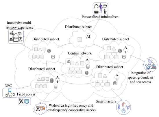
Figure 1. All technologies integrated to achieve 6G network architecture evolution.

As shown in Figure 2, the system architecture and key technologies of 6G are still in the exploration stage. Potential architecture-based technologies such as decentralized hierarchical networks with centralized and distributed collaboration, intelligent autonomous distributed management mechanisms, digital twin technology, space–ground integration, intelligent self-generation, secure self-generation, and network programmability will be integrated organically to jointly achieve the self-organization and self-evolution of 6G networks. Among them, the 6G low power and lossy network is one of the key technologies for achieving integration, wide coverage, intelligence, and greenness.

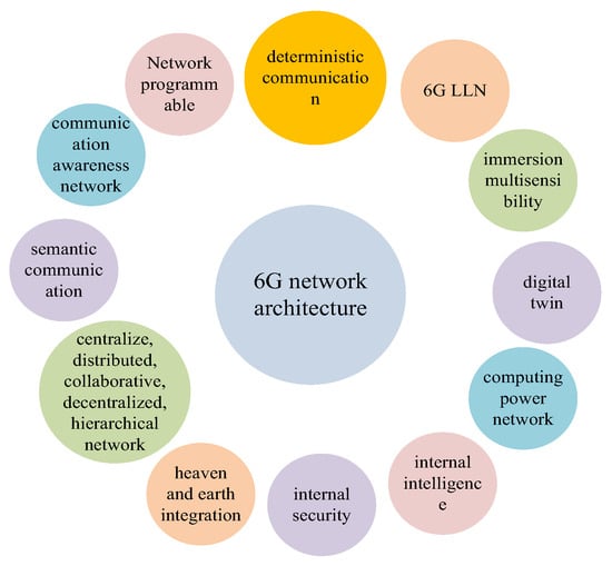
Figure 2. Various technologies are integrated to realize the evolution of 6G architecture.

The 6G low power and lossy network (LLN) [4,5] is a new type of network architecture for future Internet of Things and edge computing scenarios, aiming to solve the problem of efficient communication in resource-constrained environments. The 6G LLN, a kind of distributed network, is composed of resource-constrained nodes (such as sensors [6], wearable devices, smart terminals, etc.), which should achieve high energy efficiency and robustness in data transmission through 6G technologies (such as terahertz communication, AI-driven optimization, intelligent awareness, etc.), suitable for complex and harsh environments (such as smart cities, remote healthcare, etc.). The core characteristics of 6G LLN are low power consumption, high tolerance for lossy transmission, intelligent network topology, heterogeneous connections, edge intelligence and collaborative computing, and improvement in spectral efficiency, etc. And it can be widely used in Industry 4.0, smart agriculture, disaster rescue, smart healthcare, etc. Compared with LLN, NB-IoT, or LoRa, 6G LLN has significant improvements in energy efficiency, intelligence, and spectrum utilization and is particularly suitable for sustainable communication in complex and harsh environments.

Figure 3 shows an example of 6G LLN topology [7], which can be composed of tree-type and hybrid-type networks. Root 1–4 represent 4 different roots, 1–16 are identifiers for different nodes, DODAG 1–4 are 4 different directed non-cyclic graphs, instance 1–4 are 4 different network instances. Nodes and links in this topology are constrained in terms of computing, storage, and bandwidth; therefore, green, efficient, and reliable routing algorithms and communication mechanisms need to be designed to ensure its reliability and effectiveness.

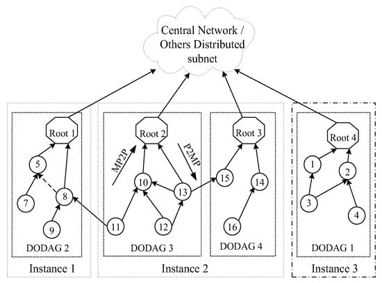
Figure 3. The 6G LLN topology instance.

2.1.2. Differences Between 6G LLN and LLN

The 6G LLN and LLN [8] share the same core goals in low power and lossy, but 6G technology introduces revolutionary enhancements. The key differences between them are listed in Table 1.

Table 1. Differences between 6G LLN and LLN.

Indicator	6G LLN	LLN
Spectrum effectiveness	THz + RIS dynamic utilization of high-frequency resources	Sub-GHz or authorized frequency band
Energy consumption management	Dynamic power consumption optimization	Fixed sleep scheduling, simple energy harvesting
Topological flexibility	Dynamic intelligent networking	Static or low-speed self-organization
Damage resistance mechanism	AI predicts channel state + federated learning optimizes redundancy	Redundant transmission, simple retransmission strategy
Delay	High delay (second level)	Higher delay (second level)
Reliability	Low	Lower
Security mechanism	Physical layer security + block chain identity authentication + quantum key distribution	Lightweight encryption
Protocol stack and architecture	AI-native protocol stack, network layer AI routing, and distributed edge intelligence	Protocol stack simplification, centralized gateway processes data
Failure recovery	Self-healing network	Manually replace the faulty node or link
Application scenarios	Digital twin, AR municipal inspection, cross-domain collaboration of deep-sea/space sensor networks, etc.	Temperature and humidity monitoring, lamp control, forest fire warning, etc.

In a word, 6G LLN is not a simple upgrade but a triple breakthrough through “intelligence + high spectrum + ultra-heterogeneous”. Therefore, its routing technology needs to be deeply optimized based on core differences such as energy efficiency, distributed autonomous decision-making, multi-dimensional routing metric evaluation strategy, broadcast suppression, protocol simplification, and intelligence. The key points that need to be focused on for 6G LLN routing technology [9,10] are shown in Table 2.

Table 2. Key points that should be considered for 6G LLN routing technology.

Indicator	6G LLN	LLN
Energy optimization	AI prediction, energy awareness	Residual energy priority
Topological flexibility	Dynamic real-time decision-making	Static or low-speed topology update
Multi-dimensional routing metric evaluation strategy	Dynamic adaptive objective function	Limited resources, crude multi-dimensional objective functions
Broadcast suppression	Opportunistic forwarding, set node forwarding conditions to reduce redundant transmission	Nodes randomly broadcast
Protocol simplification	Compress signaling header, etc., to reduce transmission load	Partial signaling redundancy
Reliability	Opportunistic forwarding, multi-dimensional routing metric evaluation	Difficult multi-dimensional routing metric evaluation
Security mechanism	Physical layer security, block chain identity authentication, and quantum key distribution	Lightweight encryption
Protocol efficiency	Hardware accelerated, ultra-minimalist signaling	6LoWPAN

According to the characteristics of 6G LLN, this paper focuses on its routing technology. The routing protocol for low power and lossy network (RPL) [11,12], standardized by the Internet Engineering Task Force (IETF), is mainly designed for LLN but is not suitable for 6G LLN. And key points listed in Table 2 should be given priority in study, since RPL was not specifically designed for 6G LLN. Therefore, in order to optimize energy consumption, improve topology flexibility, achieve multi-dimensional network QoS guarantee, set broadcast suppression conditions, simplify routing protocols, and enhance the protocol efficiency, this paper proposes an improved RPL (I-RPL) algorithm which can adapt to the characteristics of 6G LLN and meet its application requirements.

2.2. Problems Description

At present, the RPL urgently needs to improve the following problems to promote the innovation of routing technology for 6G LLN.

2.2.1. Network Topology Construction and Maintenance Technology

At present, there are relatively few technologies for researching network topology construction and maintenance. Most of them adopt the traditional LLN routing technologies construction schemes [13] (as shown in Figure 4). However, this construction scheme may encounter high control overhead, energy consumption, and low construction efficiency. Moreover, any node can become a preferred parent through broadcast DIO, but its quality may be too poor to deliver packets, which will waste energy, cache resources, and reduce the reliability of the network. In Figure 4, DIO, DIS, and DAO are control messages [14,15]; the detailed explanations are shown in Table 3.

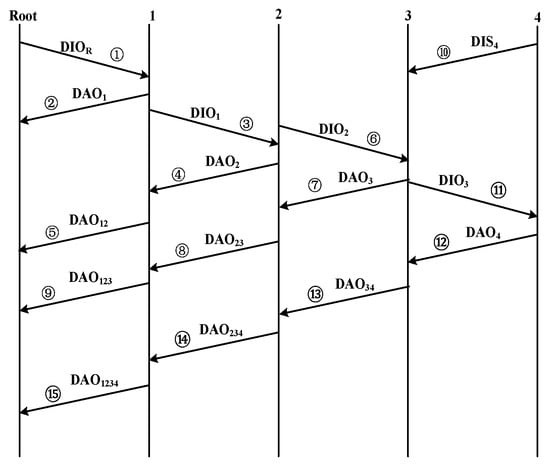
Figure 4. Simple network construction processes. (1–4 are 4 different nodes, ①–⑮ are transmission sequence of control message).

Table 3. Control message explanation.

Control Messages	Explanation
DIO	Broadcast by parents, contains information about instance and used for selecting parent set, maintaining DODAG, etc.
DIS	Solicits DIO from neighbors
DAO	Transmits destination information upward, builds uplink routing
DAO-ACK	Sent by DAO receiver to acknowledge DAO

2.2.2. Energy-Aware Routing Technologies

Routing technologies based on energy awareness can effectively prolong the network’s lifetime. Therefore, it is necessary to enhance the energy-aware and processing capabilities, provide differentiated services based on different user requirements, energy consumption prediction, and the multi-attribute decision optimization of 6G LLN routing technologies. For instance, in [16], authors integrated the Energy Efficient Multipath Routing Protocol (EM-RPL) with the Load-Based Energy Efficient RPL (EM-RPL) to address energy bottlenecks. In [17,18], they combine residual energy and several other routing metrics to determine whether the candidate parent has the ability to be the preferred parent. Each routing metric’s importance level is decided by the relevant weighting coefficient. In [19], authors proposed the QFS-RPL (Q-learning and Fisheye State RPL, QFS-RPL) algorithm, which simplifies the data transmission process to reduce the energy consumption and balance load to extend the network lifetime. In [20], authors proposed the CB-ED-RPL (Coordinator-Based Energy-Efficient Dynamic RPL, CB-ED-RPL) algorithm. CB-ED-RPL adopted a network energy-saving dynamic routing mechanism through the coordinator to achieve the efficient utilization of network energy. In addition, there are many studies, such as [21,22], that conduct research on energy consumption and the reliability of 6G LLN. However, most of them lack the scientific multi-routing metric evaluation theory and are unable to predict the energy consumption of nodes in real time. Moreover, there is no efficient and scientific method for determining the importance level of each metric.

2.2.3. Resource-Constrained Routing Technologies

In 6G LLN, nodes have limited resources in terms of storage, computing, energy, and unstable links, as well as limited bandwidth resources. Therefore, resource-constrained-oriented routing technologies should be adopted to ensure network performance. In [23], authors proposed the RT-Ranked (Resiliency TSCH/RPL Ranked, RT-Ranked) algorithm. RT-Ranked can support unexpected traffic surges to reduce control messages and load. In [24], authors proposed the TLR (Traffic-Aware Load-Balancing Routing, TLR), which can fully take into account the limitation of the cache and adopt an active path selection strategy to achieve efficient load balancing and a high throughput. In [25], authors integrated the network load and congestion conditions by an adaptive fuzzy multi-criteria decision-making approach, combining fuzzy analytic process and TOPSIS to optimize network performance. In [26], authors adopt the balancing model and ant colony algorithm to effectively balance the load and congestion. In [27], authors proposed an NIAP routing metric, which can balance the load and extend the network’s lifetime by evaluating the average energy consumption at the network interface. In [28], authors proposed the DCRL-RPL to evaluate the distance between the nodes and roots and the residual energy and load influence index to balance the load and extend the network’s lifetime.

These improvements took into account the limited network resources to a certain extent. They saved resources such as the cache and energy consumption to enhance network performance through improving routing technologies. However, some of them only focus on limited resources while neglecting the guarantee of other performance indicators. Some improvements lack the scientific theoretical framework for evaluating multi-routing metrics.

2.2.4. Calculation Method of ETX

ETX, calculated based on Equation (1), is the needed number of transmissions (re-transmissions) the node expects to successfully transmit and acknowledge a packet. In Equation (1), D_f and D_r are the probability of successfully receiving and acknowledging a packet, respectively. The path ETX is equal to the sum of link ETX.

$$ETX={\displaystyle \frac{1}{D_f\times D_r}}$$

(1)

Through evaluating ETX, the path with poor quality can be effectively avoided by selecting it as the optimal one and will improve the network reliability. At present, there are many studies about ETX, but its calculation method is rarely studied and is basically unchanged. In [29,30], authors proposed that ETX should be integrated with other routing metrics, aiming to improve the performance of network. These improvements can improve the network reliability through the in-depth study of ETX. However, some of them only focus on evaluating ETX without considering other routing metrics. Some improvements have no scientific and reasonable theoretical basis and can be used to determine the weight coefficient of each routing metric when evaluating multiple routing metrics. So, the network performance would be limited, and it is worth further study and discussion.

2.2.5. Calculation Method of Delay

A path’s delay is equivalent to the sum of the delays associated with its links. The path with high delay can be effectively avoided by selecting it as the optimal one and improving the real-time performance. At present, there are many studies about delay, but its calculation method is rarely studied and is basically unchanged. In [31], authors considered queuing and link delays by reliable and delay-efficient multi-path RPL algorithms. In [32], authors defined an extension to the Babel routing protocol that measures the round-trip time (RTT) between routers. In [33], authors selected the residual energy divided by the product of ETX and delay as the new routing metric. In [34], authors list the current research status of delay and other aspects. Although these improvements optimize the real-time performance, most of them are not evaluating other routing metrics comprehensively, lacking scientific and reasonable methods to evaluate multiple routing metrics synthetically. These problems still deserve further study and discussion.

2.2.6. Objective Function and Multiple Routing Metric Evaluation Theories

The objective function serves to define the way in which several routing metrics should be combined and converted into rank, selecting the optimal routes. In [35], authors proposed to construct the objective function by combining multiple routing metrics in lexical or additive methods. In most cases, the additive method delivers better network performance than the lexical method. However, it is a challenging task to ascertain the weighting coefficients for routing metrics when using the additive method. And most of them are based on experts’ personal subjective experiences. In [36], authors proposed an entropy-based weighted approach to assign the weights of routing metrics in the objective function. In [37], authors selected the fuzzy method to construct an objective to improve the network performance. It can be seen that weight method and fuzzy logic method are widely adopted in objective function currently. These improvements are either too subjective to objectively consider the network’s actual operation or too objective to take into account the human factors of users, control centers, etc. Meanwhile, intelligent adaptive adjustment, distributed autonomy, and QoS cannot be guaranteed. Therefore, there is no scientific, low carbon, and intelligence multiple routing metrics evaluation theory used in objective functions.

2.2.7. Preferred Parent Selection Method

At present, most of the current studies adopt the following preferred parent selection methods [38]: The node’s rank is calculated based on the objective function, and the node with the minimum (or maximum) rank can be selected as the preferred parent. If there are two or more candidate parents that have the same minimum (or maximum) rank, another different selection criteria (routing metric) will be used, or one will randomly be selected as the preferred parent. However, this random selection method may be selecting the candidate parent with a large child number or small candidate parent set as the preferred parent. In this way, the preferred parent may be heavily loaded or limit its next hop selection to some extent.

In short, the recent improvements of RPL used in 6G LLN encounter large control overhead, high energy consumption, and a lack of scientific multiple routing metric evaluation theories. Therefore, this paper proposed an improved RPL (I-RPL) algorithm to solve these problems. I-RPL designs new context-aware routing metrics, which include the residual energy indicator, buffer utilization ratio, ETX, delay, and hop. Meanwhile, the candidate parent and its preferred parent’s residual energy metric and buffer utilization ratio are calculated recursively to reduce the effect of upstream parents. And the ETX and delay calculating method are improved to ensure a better performance. Moreover, I-RPL has optimized the network construction process and designed scientific multiple routing metrics evaluation theories—Lagrangian multiplier theories, proposed new rank computing, and optimal route-selecting mechanisms. Eventually, I-RPL can select the best candidate parent as the preferred parent, acquiring major enhancements in network performance.

3. Improved RPL Algorithm (I-RPL)

3.1. Outline of I-RPL

The main contributions of I-RPL can be structured as follows:

(1)

Improved network topology construction processes.

(2)

Proposed new context-aware routing metrics (C-RM).

• Designed recursive method to evaluate the candidate parent and its preferred parent’s residual energy metric and buffer utilization ratio.
• Improved ETX and delay calculating manner.

(3)

Designed new composite context-aware objective function (C-OF).

(4)

Proposed scientific multiple routing metric evaluation theories.

(5)

Designed new rank computing and the optimal route selection mechanisms.

In the following sections, I-RPL will be elaborated based on the five parts mentioned above.

3.2. Improved Network Topology Construction Processes

I-RPL improves the network construction process to optimize network construction efficiency, reduce control overhead, and save energy consumption, etc.

3.2.1. New Mechanisms of Network Construction Processes

(1)

In the initial stage of network construction, only roots broadcast DIO; other nodes are waiting to receive DIO without sending DIS, DIO, and DAO. In this way, the control overhead and energy consumption can be reduced.

(2)

In order to ensure the quality of candidate parents, I-RPL proposed that only nodes meeting certain constraint conditions can send DIO, since these nodes may become the preferred parent and transmit packets.

(3)

Figure 5 illustrates the improved network construction processes which can improve network construction efficiency and reduce control overhead and energy consumption effectively.

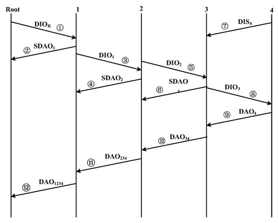Figure 5. Improved DODAG construction process. (1–4 are 4 different nodes, ①–⑫ are transmission sequence of control message).

In Figure 5, the simplified DAO (SDAO), only one bit, is used for informing the corresponding node that the sending SDAO node is ready to join the network.

3.2.2. Improved Network Construction Processes

According to Figure 5, the improved network construction processes can be detailed as follows:

Step 1: Roots broadcast DIO to its neighbors. DIO contains the necessary information for network construction and maintenance. Others are waiting to receive DIO without sending DIS, DIO, and DAO.

Step 2: Neighbors, like node 1, which receive DIO, determine if they should select the root as its parent in accordance with the objective function. If so, it will uni-cast SDAO to the root, which means that node 1 is ready to join the network and selects the root as its parent.

Step 3: After receiving the SDAO₁ sent by node 1, the root only needs to wait a certain period of time (T) to receive DAO (DAO₁₂₃₄), which contains the entire network routing and other related information. Meanwhile, node 1 re-broadcast DIO to its neighbors such as node 2. Then, node 2 performs the same operation as node 1.

Step 4: Other nodes such as node 3 perform the same operation, as above-mentioned.

Step 5: If node 4 has not received DIO from other nodes within a certain period of time, node 4 will broadcast DIS to solicit DIO from its neighbors to join the network.

Step 6: After node 4 joins the network, node 3 will uni-cast DAO₃₄, which contains the updated routing information to its parent (node 2). Then, node 2 uni-casts DAO₂₃₄ to node 1, and node 1 uni-casts DAO₁₂₃₄ to the root.

Repeat the steps stated above until the network extends coverage to all nodes.

3.2.3. Comparison and Analysis

Suppose that there are five nodes in the network, and the time required to transmit the control message (DIO, DAO, DIS, DAO-ACK, and SDAO) are the same and both are t (t > 0). According to Figure 4 and Figure 5, the time required for the original and improved network construction processes can be designed as shown in Equation (2).

$$\left\{\begin{array}{c}15t+10t, original\\ 12t+4t, improved\end{array}\right.$$

(2)

In Equation (2), 10t and 4t are the time required to replay DAO-ACK to DAO senders. Therefore, the following conclusions can be drawn:

(1)

Constructing a network with five nodes, the improved construction processes can save 3t + 6t time. And that the more nodes in the network, the more time can be saved. So, the energy consumption can be effectively reduced, and the network construction efficiency can be significantly improved.

(2)

The improved network construction processes can significantly reduce the control overhead by reducing the DAOs (and DAO-ACKs) number. And that the more nodes in the network, the more control overhead can be saved.

(3)

The time for the root to wait to receive the DAO containing the network routing and other related information can be considered as Timproved:

$$T_{improved}=\left\{\begin{array}{c}{T}_{original}-3t+\epsilon , no DAO\text{-}ACK\hfill \\ T_{original}-(3t+6t)+\epsilon , with DAO\text{-}ACK\hfill \end{array}\right.$$

(3)

In Equation (3), T_original is the time required to construct the network with five nodes using the original processes. ε is a small positive number. So, the network construction efficiency can also be optimized. And the more nodes in the network, the more the network construction efficiency can be improved.

3.3. New Context-Aware Routing Metrics (C-RM)

To satisfy the application requirements of 6G LLN, the new composite context-aware routing metric (C-RM), which simultaneously considers the residual energy indicator, buffer utilization ratio, expected transmission count (ETX), delay, and hop count, is proposed. C-RM recursively calculates the candidate parent and its preferred parent’s residual energy metric and buffer utilization ratio to reduce the effect of upstream parents, since further paths are evaluated. Meanwhile, C-RM optimizes ETX and the delay calculating method through a comprehensive application sum and the mean and standard deviation of ETX and delay to ensure a better performance. In the following, routing metrics used in C-RM are designed. Suppose node c has n candidate parents.

3.3.1. Residual Energy Indicator (REI)

REI is the residual energy indicator of nodes and can be calculated based on Equation (4).

$${\eta }_1(i)=REI(i)=\left\{\begin{array}{c}{\displaystyle \frac{E_{initial}(i)-E_{current}(i)}{E_{initial}(i)}} i=root\\ Max({\displaystyle \frac{E_{initial}(i)-E_{current}(i)}{E_{initial}(i)}}, {\eta }_1(i_p)\times {\tau }_1) i\ne root, i=1,2,\cdots ,n\end{array}\right., 0\le {\eta }_1(i)\le 1$$

(4)

In Equation (4), E_initial(i) and E_current(i) are the initial and current energy of candidate parent i. i_p is the preferred parent (the next hop) of candidate parent i. τ₁, the adjustment parameter, is used for reducing the energy condition of parents so that the energy consumption effect does not go farther than some degree. Its value is a random number in [0, 1]. REI(i) is the residual energy indicator of the candidate parent (neighbor) i and its preferred parent i_p. In other words, REI(i) evaluates the remaining energy of nodes recursively. And the impact of the parent node’s remaining energy becomes weaker as it moves farther down the path. Therefore, REI can be used to avoid choosing paths with low remaining energy to transmit packets.

3.3.2. Buffer Utilization Ratio (BUR)

Buffer utilization ratio represents the buffer occupancy of nodes and can be evaluated according to Equation (5). Q(i) is the buffer usage indicator and can be calculated based on Equation (6). i_p is the preferred parent of candidate parent i. τ₂, the adjustment parameter, is used for reducing the buffer utilization condition of parents so that the buffer utilization effect does not go farther than some degree. Its value is a random number in [0, 1]. BUR(i) reflects the buffer utilization ratio of candidate parent i and its preferred parent i_p. In other words, BUR(i) evaluates the buffer utilization ratio of nodes recursively. And the effect of parent buffer utilization is less when it gets farther down the path. Therefore, BOR can be used to relieve congestion and balance the load.

$$\begin{array}{l}{\eta }_2(i)=BUR(i)=\left\{\begin{array}{c}Q(i) i=root\\ Max(Q(i), {\eta }_2(i_p)\times {\tau }_2) i\ne root, i=1,2,\cdots ,n\end{array}\right.\hfill \\ 0\le {\eta }_2(i)\le 1\hfill \end{array}$$

(5)

$$Q(i)={\displaystyle \frac{packets number in node (i) buffer}{total buffer size of node (i)}}, 0\le Q(i)\le 1$$

(6)

3.3.3. ETX

According to Equation (1), the ETX of a link can be calculated, and then the total ETX of a path can be obtained through summing all the links’ ETX. When transmitting data packets, the optimal path can be selected as the one with the smallest ETX. But the optimal path may include a long single hop, which is a bottleneck of the whole network. Therefore, C-RM proposes using the sum, mean, and standard deviation of ETX comprehensively. First, suppose that ${\sigma }_{ETX}(i), ETX(i)$, $\overline{ETX}(i)$ are the ETX standard deviation, sum, and mean of links in the path from node c through candidate parent i to the root and can be calculated based on Equation (7). h_i is the hop count of path P_i from node c through candidate parent i to the root. Then, the specific usage rules of ETX are as follows:

Step 1: Calculating ${\sigma }_{ETX}(i), ETX(i), \overline{ETX}(i)$ of path P_i.

Step 2: Arranging ETX(i) values in ascending order, then combining the paths corresponding to the minimum first three ETX(i) values into the alternative path set. If less than three paths, then all of them are selected into the alternative path set.

Step 3: The path with the minimum ${\sigma }_{ETX}(i)$ will be selected as the optimal path. For instance, suppose ${\sigma }_{ETX}(f)$ is the minimum value, then the path P_f (the path from node c through candidate parent f to the root) is the optimal one. So, f is the preferred parent of c.

Clearly, using the sum, mean, and standard deviation of ETX in a comprehensive manner not only ensures link quality but also avoids choosing the optimal path with high-ETX links. Normalization is required to facilitate the integration of ETX and other routing metrics, which is shown in Equation (8).

$$\begin{array}{c}{\sigma }_{ETX}(i)=\sqrt{{\displaystyle \frac{1}{h_i-1}}{\displaystyle \sum _{k=1}^{h_i}{(ET{X}_k-{\overline{ETX}}_i)}^2}}\\ \overline{ETX}(i)={\displaystyle \frac{ET{X}_i}{h_i}}\\ ETX(i)=ET{X}_1+ET{X}_2+,\cdots ,+ET{X}_{h_i}\end{array}$$

(7)

$${\eta }_3(i)=\left\{\begin{array}{c}0 i=root\hfill \\ \underset{normalization}{{\sigma }_{ETX}(i)} i\ne root\hfill \end{array}\right., \underset{normalization}{{\sigma }_{ETX}(i)}={\displaystyle \frac{{\sigma }_{ETX}(i)}{{\displaystyle \sum _{i=1}^n{\sigma }_{ETX}(i)}}}, 0\le \underset{normalization}{{\sigma }_{ETX}(i)}\le 1, (i=1,2,\cdots ,n)$$

(8)

3.3.4. Delay (D)

As shown in Section 2.2.5, it is problematic to calculate the delay of a path in a summation manner. The reason is that the ultimately selected path may include one or more links experiencing a large delay. Therefore, this paper proposes to comprehensively use the sum, mean, and standard deviation of each link’s delay in a path. First, suppose that ${\sigma }_D(i), D(i), \overline{D}(i)$ are the delay standard deviation, sum, and mean of links in the path from node c through candidate parent i to the root and can be calculated based on Equation (9). h_i is the hop count of path P_i from node c through candidate parent i to the root. Then, the specific usage rules of delay are as follows:

Step 1: Calculating ${\sigma }_D(i), D(i), \overline{D}(i)$ of path P_i.

Step 2: Arranging D(i) values in ascending order, then combine the paths corresponding to the minimum first three D(i) values into the alternative path set. If the number of paths is fewer than three, all such paths should be incorporated into the alternative path set.

Step 3: The path with the minimum ${\sigma }_D(i)$ will be selected as the optimal path. For instance, suppose ${\sigma }_D(f)$ is the minimum value, then the path P_f (the path from node c through candidate parent f to the root) is the optimal one. So, f is the preferred parent of c.

It is obvious that comprehensively using the sum, mean, and standard deviation of delay not only ensures delay performance but also avoids selecting the optimal path with high delay links. For the convenience of combining delay with other routing metrics, normalization is required, as shown in Equation (10).

$$\begin{array}{c}{\sigma }_D(i)=\sqrt{{\displaystyle \frac{1}{h_i-1}}{\displaystyle \sum _{k=1}^{h_i}{(D_k-{\overline{D}}_i)}^2}}\\ D(i)=D_1+D_2+,\cdots ,+D_{h_i}\\ \overline{D}(i)={\displaystyle \frac{D_i}{h_i}}\end{array}$$

(9)

$${\eta }_4(i)=\left\{\begin{array}{c}0 i=root\hfill \\ \underset{normalization}{{\sigma }_D(i)} i\ne root\hfill \end{array}\right., \underset{normalization}{{\sigma }_D(i)}={\displaystyle \frac{{\sigma }_D(i)}{{\displaystyle \sum _{i=1}^n{\sigma }_D(i)}}}, 0\le \underset{normalization}{{\sigma }_D(i)}\le 1, (i=1,2,\cdots ,n)$$

(10)

3.3.5. Hop Count

Hop count refers to the number of hops between a candidate parent and the root. It helps avoid choosing candidate parents with more hops to transmit packets. As the hop count has been incorporated into the calculation of ETX and delay standard deviation, the hop count is not considered separately in this paper.

In a word, C-RM recursively evaluates REI and BOR, using the ETX and delay sum, mean, and standard deviation to ensure a better performance of 6G LLN.

3.4. New Composite Context-Aware Objective Function (C-OF)

The composite objective function can be designed as Equation (11). It combines REI, BOR, ETX, and D in an additive method. And w₁, w₂, w₃, and w₄ are weighting coefficients, which are used to adjust the importance of each routing metric. n is the number of candidate parents and $\underset{Composition}{F(i)}$ is the composite objective function of the i-th candidate parent.

$$\underset{Composition}{F(i)}={\displaystyle \sum _{j=1}^m{w}_j}{\eta }_j(i), s.t. \left\{\begin{array}{c}{\displaystyle \sum _{j=1}^m{w}_j}=1\\ 0\le w_j\le 1\end{array}\right., (i=1,2,\cdots ,n)$$

(11)

Then, C-OF can be designed as the minimum value of $\underset{Composition}{F(i)}$, as illustrated in Equation (12).

$$CP\text{-}OF=\min \underset{Composition metric}{F(i)}=\min ({\displaystyle \sum _{j=1}^m{w}_j}{\eta }_j(i)), s.t. \left\{\begin{array}{c}{\displaystyle \sum _{j=1}^m{w}_j}=1\\ 0\le w_j\le 1\end{array}\right., (i=1,2,\cdots ,n)$$

(12)

It can be seen that C-OF can comprehensively evaluate the REI, BOR, ETX, and D of candidate parents. And the weighting coefficients can be used to adjust the importance of corresponding routing metrics to further affect the evaluation results. Therefore, it is a key problem to determine the weight coefficients of routing metrics reasonably and effectively. I-RPL proposes Lagrangian multiplier theories to determine the weighting coefficients of routing metrics. Lagrangian multiplier theories synthesize the subjective (Fuzzy Analytic Hierarchy Process, FAHP) and objective (entropy method) weighting coefficient determination methods. This scientific multiple routing metrics evaluation theory comprehensively applied the advantage of the subjective and objective weighting method and can select the most suitable candidate parent as the preferred parent. Thus, the network performance can be significantly improved.

3.5. Novel Scientific Multiple Routing Metric Evaluation Theories

Supposing that node c has n candidate parents, x_ij is the value of the j-th routing metric for the i-th candidate parent. Then, the sample set of each routing metric value at every candidate parent is $\left\{x_{ij}\left|i=1,2,\cdots ,n; j=1,2,\cdots ,m\right.\right\}$. It can be represented as initial matrix X.

$$X=\left[\begin{array}{ccccc}{x}_{11}& x_{12}& x_{13}& \cdots & x_{1m}\\ x_{21}& x_{22}& x_{23}& \cdots & x_{2m}\\ \cdots & \cdots & \cdots & \cdots & \cdots \\ x_{n1}& x_{n2}& x_{n3}& \cdots & x_{nm}\end{array}\right]$$

(13)

Then, according to Equation (11), the comprehensive evaluation function of candidate parents can be designed as Equation (14).

$$\begin{array}{l}F(i)={\displaystyle \sum _{j=1}^m{w}_j{\eta }_j(i)={\displaystyle \sum _{j=1}^m{w}_j\times x_{ij}}}\\ s.t. \left\{\begin{array}{c}{\displaystyle \sum _{j=1}^m{w}_j}=1\\ 0\le w_j\le 1\end{array}\right., x_{ij}={\eta }_j(i), i=1,2,\cdots ,n, m=4\end{array}$$

(14)

Therefore, according to the reasonable and scientific weighting coefficients of routing metrics, the comprehensive evaluation results of candidate parents (F(i)) can be obtained. Then, the one with the minimum value of Equation (14) can be chosen as the preferred parent. I-RPL proposed scientific multiple routing metric evaluation theories—Lagrangian multiplier theories, which synthetically utilize the subjective (FAHP) and objective (entropy method) weighting methods to select the optimal path.

3.5.1. Subjective Weighting Method

AHP compares the importance degree, possibility degree, and preference degree of attributes of evaluators through the scale, quantifies the processing, establishes the mathematical model, and solves it. FAHP [39] is a decision-making method based on AHP. It introduces the fuzzy consistency matrix for the fuzziness of people’s judgment on complex things. FAHP solves the consistency problem of the AHP judgment matrix well. But this method is too subjective. Before introducing FAHP, the following definitions are given:

Definition 1.

For matrix $R={(r_{ij})}_{n\times m}$, if $0\le r_{ij}\le 1$, then R is the fuzzy matrix.

Definition 2.

For matrix $R={(r_{ij})}_{n\times m}$, if $r_{ij}+r_{ji}=1$, then R is the fuzzy complementary matrix.

Definition 3.

For fuzzy matrix $R={(r_{ij})}_{n\times m}$, $\forall g$, if $r_{ij}=r_{ig}-r_{jg}+0.5$, then R is the fuzzy consistency matrix.

The specific steps of the subjective weighting method based on FAHP are as follows:

Step 1: Constructing the evaluation hierarchy analysis model.

Figure 6 illustrates the hierarchical evaluation model. The objective layer, at the top of the hierarchical evaluation model, is the ultimate decision-making goal. The criterion layer, at the middle of the hierarchical evaluation model, consists of several evaluation criterion, which are need to be considered (routing metrics). The scheme layer, at the bottom of the hierarchical evaluation model, consists of evaluated objects (candidate parents).

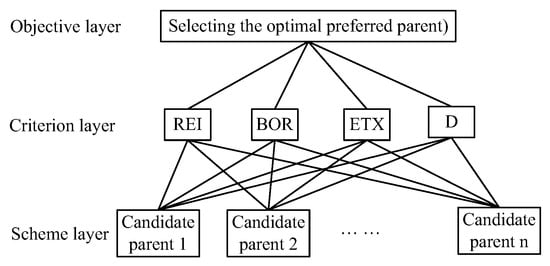
Figure 6. AHP hierarchical evaluation model.

Step 2: Calculating the weight vector.

(a) Constructing the fuzzy judgment matrix $R={(r_{ij})}_{n\times m}$.

In $R={(r_{ij})}_{n\times m}$, r_ij represents the correlation degree of the fuzzy relationship between the i-th element and j-th element. In order to quantitatively describe the relative importance between any two routing metrics, this paper adopts the scale of 0.1–0.9, as shown in Table 4.

Table 4. Scale of 0.1–0.9.

Scale	Variance Position
0.5	Both elements are equally important
0.6	One element is slightly more important than the other
0.7	One element is more important than the other
0.8	One element is strongly more important than the other
0.9	One element is extremely more important than the other
0.1–0.4	The counter comparison, if rij can be obtained through ri compared with rj, then 1-rij can be obtained through rj compared with ri

(b) Calculating the fuzzy consistency matrix R’.

The fuzzy consistency matrix R’ can be calculated by Equations (15) and (16). Moreover, the consistency checks during the matrix change processes can be avoided by Equation (15).

$${\xi }_i={\displaystyle \sum _{j=1}^m{r}_{ij}}; i=1,2,\cdots ,n$$

(15)

$${\xi }_{ij}={\displaystyle \frac{{\xi }_i-{\xi }_j}{2n}}+0.5$$

(16)

(c) Calculating the weight vector.

The row sum normalization of the fuzzy consistency matrix R’ can be calculated based on Equation (17), and then the weight vector $w^{FAHP}=(w_1^{FAHP}, w_2^{FAHP},\cdots , w_m^{FAHP})$ can be obtained.

$$w_i^{FAHP}=({\displaystyle \sum _{j=1}^m{r}_{ij}})/{\displaystyle \sum _{i=1}^n{\displaystyle \sum _{j=1}^m{r}_{ij}}}$$

(17)

According to the above-mentioned steps of FAHP, the concrete operations of calculating routing metrics’ subjective weight coefficients can be summarized as follows:

Operation 1.

Constructing the fuzzy judgment matrix R.

According to Figure 7 and Table 3, the fuzzy judgment matrix R can be constructed as shown in Equation (18).

$$\begin{array}{c} REI BOR ETX D\hfill \\ R=\begin{array}{c}REI\\ BOR\\ ETX\\ D\end{array}\left[\begin{array}{cccc}0.5& 0.4& 0.3& 0.7\\ 0.6& 0.5& 0.4& 0.7\\ 0.7& 0.6& 0.5& 0.8\\ 0.3& 0.3& 0.2& 0.5\end{array}\right]\end{array}$$

(18)

Operation 2.

Calculating the fuzzy consistency matrix R’.

According to Equations (15) and (16), the fuzzy consistency matrix R’ can be calculated as shown in Equation (19).

$$R^{’}=\left[\begin{array}{cccc}0.5& 0.4625& 0.4125& 0.575\\ 0.5375& 0.5& 0.45& 0.6125\\ 0.5875& 0.55& 0.5& 0.6625\\ 0.425& 0.3875& 0.3375& 0.5\end{array}\right]$$

(19)

Operation 3.

Calculating the weight vector.

According to Equation (17), the weight coefficients of routing metrics can be obtained, as shown in Equation (20).

$$w^{FAHP}=(w_1^{FAHP}, w_2^{FAHP},\cdots , w_m^{FAHP})=(0.24375, 0.2625, 0.2875, 0.20625)$$

(20)

Operation 4.

Calculating C-OF in the FAHP method.

According to Equation (12), the objective function (C-OF) value of candidate parent i in the FAHP method can be represented as follows:

$$\begin{array}{l}\underset{FAHP}{N-OF}=\min ({\displaystyle \sum _{j=1}^4{w}_j^{FAHP}}{\eta }_j(i))\\ =\min (0.24375{\eta }_1(i)+ 0.2625{\eta }_2(i) + 0.2875{\eta }_3(i)+0.20625{\eta }_4(i))\end{array}$$

(21)

Then, the candidate parent with the minimum value of Equation (21) can be selected as the preferred parent.

3.5.2. Objective Weighting Method

The entropy method [40,41] calculates weighting coefficients by extracting the information entropy value of the indicator change based on the concept of entropy in information theory. Its basic idea is calculating the weight coefficient of each indicator according to relative importance of indicators, concept, and nature of entropy. If the information entropy of an indicator is small, the variation degree of this indicator is relatively large, which contains a large amount of information, plays a greater role, and a larger weighting coefficient should be allocated. On the contrary, if the information entropy of an indicator is large, a smaller weighting coefficient should be allocated. The entropy method is not affected by the subjective factors of evaluators and can reflect the relationship between indicator change and indicator weight well. It is an ideal objective weighting method. The concrete steps of calculating indicator weight by entropy method are as follows:

Step 1: Calculating proportion P_ij of the indicator value for the i-th evaluated object at the j-th indicator in the initial matrix (Equation (13)), based on Equation (22).

$$P_{ij}={\displaystyle \frac{x_{ij}}{{\displaystyle \sum _{i=1}^n{x}_{ij}}}}, i=1,2,\cdots ,n, j=1,2,\cdots ,m$$

(22)

In Equation (22), n is the number of candidate parents of node c, m = 4 is the number of evaluated routing metrics.

Step 2: Calculating the entropy value E_j of the j-th indicator (routing metric), according to Equation (23).

$$E_j=-k{\displaystyle \sum _{i=1}^n{p}_{ij}Ln{p}_{ij}}, k={\displaystyle \frac{1}{\ln n}}, 0\le E_j\le 1$$

(23)

Step 3: Calculating the difference coefficient d_j of the j-th indicator, based on Equation (24).

$$d_j=1-E_j$$

(24)

Step 4: Normalizing d_j according to Equation (25) and then obtaining the weighting coefficients of routing metrics $w_j^{entropy}$.

$$w_j^{entropy}={\displaystyle \frac{d_j}{{\displaystyle \sum _{j=1}^m{d}_j}}}$$

(25)

Then, according to Equation (12), the C-OF value of the candidate parent i in the entropy method can be designed as follows:

$$\underset{entropy}{N\text{-}OF}=\min ({\displaystyle \sum _{j=1}^4{w}_j^{entropy}}{\eta }_j(i))$$

(26)

Then by the entropy method, the candidate parent with the minimum value of Equation (26) can be selected as the preferred parent.

3.5.3. Lagrangian Multiplier Theories

I-RPL synthesizes the entropy method and FAHP to realize the complementary advantages of subjective and objective methods and obtain a better performance. In order to obtain scientific multiple routing metric evaluation results, it is necessary to calculate the influence of the entropy method and FAHP according to certain methods. I-RPL proposed Lagrangian multiplier theories. And the detailed steps of synthesizing the entropy method and FAHP through Lagrangian multiplier theories are as follows:

Step 1: Constructing the synthesized weight mathematical model.

The synthesized weight mathematical model can be constructed as Equation (27). w_j is the synthesized weight of the j-th routing metric. $w_j^{(k)}$ is the weight of the j-th routing metric by the k-th weighting determination method. ${\alpha }_k$ is weighting coefficient of the weight determined by the k-th weighting determination method.

$$\begin{array}{c}{w}_j={\alpha }_1{w}_j^{(1)}+{\alpha }_2{w}_j^{(2)}+\cdots +{\alpha }_k{w}_j^{(k)}={\displaystyle \sum _{\tau =1}^k{\alpha }_{\tau }{w}_j^{(\tau )}}\\ s.t.{\displaystyle \sum _{\tau =1}^k{\alpha }_{\tau }^2}=1\end{array}$$

(27)

Step 2: Constructing the fitness function.

According to Equation (14), the fitness function f(i) can be constructed as shown in Equation (28). f(i) is the fitness function value of the i-th candidate parent. x_ij is the normalized value of the j-th routing metric of the i-th candidate parent.

$$f(i)={\displaystyle \frac{1}{1+F(i)}} ={\displaystyle \frac{1}{1+{\displaystyle \sum _{j=1}^m{x}_{ij}\times [{\displaystyle \sum _{\tau =1}^k{\alpha }_{\tau }\times w_j^{\tau }}]}}}$$

(28)

Step 3: Constructing the linear programming model and optimization model.

According to Equation (28), the linear programming model of F(i) can be constructed as Equation (29).

$$\begin{array}{c}\min F(i)=(F(1), F(2),\cdots ,F(n))\\ s.t.\left\{\begin{array}{c}{a}_{\tau }>0\\ {\displaystyle \sum _{\tau =1}^k{a}_{\tau }^2=1}\end{array}\right.\end{array}$$

(29)

The optimization model can be constructed as Equation (30).

$$\begin{array}{c}\min F=A[B{(\alpha w)}^T]={\left(\begin{array}{c}1\\ 1\\ \cdots \\ 1\end{array}\right)}_{n\times 1}^T\times \left\{\left(\begin{array}{cccc}{x}_{11}& x_{12}& \cdots & x_{1m}\\ x_{21}& x_{22}& \cdots & x_{2m}\\ \cdots & \cdots & \cdots & \cdots \\ x_{n1}& x_{n2}& \cdots & x_{nm}\end{array}\right){\left[{\left(\begin{array}{c}{\alpha }_1\\ {\alpha }_2\\ \cdots \\ {\alpha }_k\end{array}\right)}^T\times \left(\begin{array}{cccc}{w}_1^{(1)}& w_2^{(1)}& \cdots & w_m^{(1)}\\ w_1^{(2)}& w_2^{(2)}& \cdots & w_m^{(2)}\\ \cdots & \cdots & \cdots & \cdots \\ w_1^{(k)}& w_2^{(k)}& \cdots & w_m^{(k)}\end{array}\right)\right]}^T\right\}\\ s.t.\left\{\begin{array}{c}{a}_{\tau }>0, (\tau =1, 2,\cdots , k)\\ {\displaystyle \sum _{\tau =1}^k{a}_{\tau }^2=1}\end{array}\right.\end{array}$$

(30)

Step 4: Calculating ${\alpha }_{\tau }$ and $\lambda$ through constructing a function based on Lagrangian multiplier theories.

(a) Constructing a function based on Lagrangian multiplier theories.

The constructed function based on Lagrangian multiplier theories is shown in Equation (31).

$$L=f({\alpha }_{\tau }, \lambda )=A[B{(\alpha w)}^T]-{\displaystyle \frac{1}{2}}\lambda \left({\displaystyle \sum _{\tau =1}^k{\alpha }_{\tau }^2-1}\right)$$

(31)

(b) Calculating partial derivatives of ${\alpha }_{\tau }$ and $\lambda$ in Equation (31), the corresponding expressions are as follows:

$${\displaystyle \frac{\partial f}{\partial {\alpha }_1}}={\displaystyle \sum _{i=1}^n{\displaystyle \sum _{j=1}^m{x}_{ij}\times w_j^{(1)}}}-\lambda {\alpha }_1=0$$

(32)

$${\displaystyle \frac{\partial f}{\partial {\alpha }_2}}={\displaystyle \sum _{i=1}^n{\displaystyle \sum _{j=1}^m{x}_{ij}\times w_j^{(2)}}}-\lambda {\alpha }_2=0$$

(33)

$${\displaystyle \frac{\partial f}{\partial {\alpha }_k}}={\displaystyle \sum _{i=1}^n{\displaystyle \sum _{j=1}^m{x}_{ij}\times w_j^{(k)}}}-\lambda {\alpha }_k=0$$

(34)

$${\displaystyle \frac{\partial f}{\partial \lambda }}={\displaystyle \sum _{\tau =1}^k{\alpha }_{\tau }^2}-1=0$$

(35)

(c) Calculating ${\alpha }_{\tau }, (\tau =1, 2,\cdots ,k)$.

As shown in Equation (36), ${\alpha }_{\tau }^2$ can be calculated through summing the squares of derivative functions of ${\alpha }_{\tau }$, such as Equations (32)–(34).

$${\alpha }_{\tau }^2={\displaystyle \frac{{\left[{\displaystyle \sum _{i=1}^n{\displaystyle \sum _{j=1}^m{x}_{ij}{w}_j^{(\tau )}}}\right]}^2}{{\lambda }^2}}$$

(36)

Then, Equation (37) can be derived based on Equation (36).

$${\displaystyle \sum _{\tau =1}^k{\alpha }_{\tau }^2}={\displaystyle \sum _{\tau =1}^k\frac{{\left[{\displaystyle \sum _{i=1}^n{\displaystyle \sum _{j=1}^m{x}_{ij}{w}_j^{(\tau )}}}\right]}^2}{{\lambda }^2}}$$

(37)

After that, based on Equations (35) and (37), (38) can be derived.

$${\displaystyle \sum _{\tau =1}^k{\alpha }_{\tau }^2}-1={\displaystyle \sum _{\tau =1}^k\frac{{\left[{\displaystyle \sum _{i=1}^n{\displaystyle \sum _{j=1}^m{x}_{ij}{w}_j^{(\tau )}}}\right]}^2}{{\lambda }^2}}-1=0$$

(38)

So ${\alpha }_{\tau }$ can be represented as Equation (39).

$${\alpha }_{\tau }={\displaystyle \frac{{\displaystyle \sum _{i=1}^n{\displaystyle \sum _{j=1}^m{x}_{ij}{w}_j^{(\tau )}}}}{\lambda }}$$

(39)

(d) Normalizing ${\alpha }_{\tau }$.

As shown in Equation (40), ${\alpha }_{\tau }^{*}$ is the normalized expression of ${\alpha }_{\tau }$.

$${\alpha }_{\tau }^{*}={\displaystyle \frac{{\displaystyle \sum _{i=1}^n{\displaystyle \sum _{j=1}^m{x}_{ij}{w}_j^{(\tau )}}}}{{\displaystyle \sum _{\tau =1}^k{\displaystyle \sum _{i=1}^n{\displaystyle \sum _{j=1}^m{x}_{ij}{w}_j^{(\tau )}}}}}}$$

(40)

Step 5: Calculating the synthesized weight.

According to Equations (27) and (40), the synthesized weight can be calculated.

There are two kinds of weight determination methods (FAHP and entropy) designed in I-RPL, so k = 2, supposing that ${\alpha }_1^{*}={\alpha }_{FAHP}^{*}$ and ${\alpha }_2^{*}={\alpha }_{entropy}^{*}$. Therefore, the expression of synthesized weight can be constructed as Equation (41).

$$\begin{array}{l}{w}_j={\alpha }_1^{*}{w}_j^{(1)}+{\alpha }_2^{*}{w}_j^{(2)}={\alpha }_{FAHP}^{*}{w}_j^{FAHP}+{\alpha }_{entropy}^{*}{w}_j^{entropy}\\ {\alpha }_1^{*}={\alpha }_{FAHP}^{*}={\displaystyle \frac{{\displaystyle \sum _{i=1}^n{\displaystyle \sum _{j=1}^4{x}_{ij}{w}_j^{(FAHP)}}}}{{\displaystyle \sum _{i=1}^n{\displaystyle \sum _{j=1}^4{x}_{ij}{w}_j^{(FAHP)}}}+{\displaystyle \sum _{i=1}^n{\displaystyle \sum _{j=1}^4{x}_{ij}{w}_j^{(entropy)}}}}}\\ {\alpha }_2^{*}={\alpha }_{entropy}^{*}={\displaystyle \frac{{\displaystyle \sum _{i=1}^n{\displaystyle \sum _{j=1}^4{x}_{ij}{w}_j^{(entropy)}}}}{{\displaystyle \sum _{i=1}^n{\displaystyle \sum _{j=1}^4{x}_{ij}{w}_j^{(FAHP)}}}+{\displaystyle \sum _{i=1}^n{\displaystyle \sum _{j=1}^4{x}_{ij}{w}_j^{(entropy)}}}}}\end{array}$$

(41)

3.5.4. Multiple Routing Metrics Evaluation Theories

The specific processes of calculating the fitness function and C-OF by multiple routing metric evaluation theories can be summarized as follows:

Process 1: Calculating the subjective weight.

FAHP is designed to be used as a subjective weighting method to calculate the weighting coefficients of routing metrics. Its concrete operations are listed in “Section 3.5.1”.

Process 2: Calculating the objective weight.

The entropy method is designed to be used as the objective weighting method to calculate the weighting coefficients of routing metrics. Its concrete operations are listed in “Section 3.5.2”.

Process 3: Calculating the synthesized weighting coefficients.

The synthesized weighting coefficient ${\alpha }_{\tau }$ can be calculated based on Lagrangian multiplier theories, and the concrete operations are listed in “Section 3.5.3”. Then the normalized combination weighting coefficients ${\alpha }_{\tau }$ can be obtained.

Process 4: Calculating the synthesized weight w_j.

The synthesized weight w_j can be obtained through Equation (41).

Process 5: Calculating the fitness function and C-OF.

According to Equation (41), the fitness function and C-OF of the candidate parent i can be calculated as Equations (42) and (43).

$$f(i)={\displaystyle \frac{1}{1+F(i)}}={\displaystyle \frac{1}{1+{\displaystyle \sum _{j=1}^m{x}_{ij}\times w_j}}} ={\displaystyle \frac{1}{1+{\displaystyle \sum _{j=1}^4{x}_{ij}\times ({\alpha }_{FAHP}^{*}{w}_j^{FAHP}+{\alpha }_{entropy}^{*}{w}_j^{entropy})}}}$$

(42)

$$N\text{-}OF=\min \underset{Composition metric}{F(i)}=\min ({\displaystyle \sum _{j=1}^m{w}_j}{\eta }_j(i))=\min ({\displaystyle \sum _{j=1}^4({\alpha }_{FAHP}^{*}{w}_j^{FAHP}+{\alpha }_{entropy}^{*}{w}_j^{entropy})\times }{\eta }_j(i))$$

(43)

In Equations (42) and (43), ${\alpha }_{FAHP}^{*}$ and ${\alpha }_{entropy}^{*}$ can be obtained depending on Equation (41), and $w_j^{FAHP}$ and $w_j^{entropy}$ can be obtained depending on Equations (20) and (25). So, the one with the maximum value of Equation (42) or the minimum value of Equation (43) can be selected as the preferred parent. Therefore, I-RPL can acquire major enhancements in network performance.

In a word, multiple routing metric evaluation theories synthesize the advantages of subjective and objective weighting methods. It not only overcomes the problem that the subjective weighting method cannot consider the objective application requirements of 6G LLN but also solves the problem that the objective weighting method cannot consider the subjective preference factors of users. Therefore, I-RPL can significantly improve network performance. In addition, this theory provides a certain theoretical basis for multiple routing metric evaluations in the 6G LLN routing algorithm and other fields which need to evaluate multiple indicators.

3.6. Complexity Analysis of N-OF

The computational complexity of OF is influenced by multiple key factors together, such as candidate parent number, dimension of the optimization problem and convergence criterion, and so on.

Suppose that n is the candidate parent number, m = 4 is the dimension of the optimization problem, then the computational complexity of OF in I-RPL can be represented as O(nm). Due to the low value of m, its complexity is approximately O(n). It can be seen that the computational complexities of I-RPL and RPL improvements are mainly related to the candidate parent number and the dimension of optimization problem and are basically the same. Therefore, I-RPL can ensure network performances without incurring additional computational complexity.

3.7. Novel Rank Calculating Method

A node’s rank represents where it is located in relation to the root. In order to avoid loop, rank strictly increases in the Down direction (the direction from the root towards the leaf nodes) and decreases in the Up direction (the direction from the leaf nodes to the root). The rank of a node can be calculated based on OF. In I-RPL, we proposed a novel rank calculated method based on C-OF.

In I-RPL, the rank of the root is set 1.0. For other non-root nodes such as node c, the calculating method is based on Equation (44).

$$R_c(i)=R_{cp}(i)+R(i), R(i)=F(i)+1$$

(44)

In Equation (44), R_cp(i), advertised by candidate parent i through DIO, is the rank of i. R(i) is the C-OF value of the link which is from c to the candidate parent i. R_c(i) is the rank of c, which is based on the route from c through candidate parent i to the root.

According to Equation (44), the values of $\{R_c\left(1\right), R_c\left(2\right),\cdots , R_c\left(\mathrm{n}\right)\}$ can be obtained. If $\min \{R_c\left(1\right), R_c\left(2\right),\cdots , R_c\left(\mathrm{n}\right)\}=R_c(f)$, then f can be selected as the preferred parent.

3.8. Novel Preferred Parent Selection Method

According to Section 3.7, it can be seen that candidate parent f with the minimum value of Equation (44) can be selected as the preferred parent. However, this preferred parent selection method is not applicable to all cases. For example, if two or more candidate parents have the same and minimum rank, it is difficult to select the preferred parent, according to Section 3.7. Therefore, the novel preferred parent selecting mechanism is proposed:

(1)

If the rank of a candidate parent is equal to or less than that of current preferred parent, but the difference between them is less than replacing the preferred parent threshold, then the current preferred parent will not be replaced. This operation can guarantee the topology stability of 6G LLN without affecting the network performance.

(2)

If the rank of a candidate parent, calculated according to Equation (44), is less than 1.0 or greater than the node number in 6G LLN, then this candidate parent must be eliminated from the candidate parent set. Since the quality of this candidate parent is so bad, it is unable to deliver any packets or its rank is calculated incorrectly and it needs to be rejoined to the candidate parent set or become a leaf.

(3)

When conducting preferred parent selection, if ranks of two or more candidate parents are equal and minimum, then the one whose candidate parent set is the largest will be selected to serve as the preferred parent. If there are multiple candidate parents whose candidate parent sets are the largest and equal, then one is randomly selected as the preferred parent. Because the larger the candidate parent set is, the larger the preferred parent selection range is, and the more likely it is to select the optimal one as the preferred parent.

(4)

If the candidate parent set of c has only 1 node, then c waits for a period of time so that more nodes may join its candidate parent set. Then, if the candidate parent set of c is greater than or equal to 2, c selects its preferred parent by executing the I-RPL algorithm. Otherwise, c directly chooses this candidate parent as its preferred parent without executing the I-RPL algorithm, and the rank of c is equal to the rank of this candidate parent plus 1.

4. Performance Evaluation

To quantitatively evaluate and compare the new proposed I-RPL algorithm and several popular improvements of RPL, such as ETXOF, AHP, entropy, and OF0, we carry out a series of experiments by OPNET14.5.

4.1. The Selected Statistic Metrics

This paper selects seven important statistic metrics, as illustrated in Table 5, to comprehensively evaluate and compare the performance of I-RPL and its several popular improvements.

Table 5. The selected statistic metrics.

Statistic Metrics	Explanations	Formula
Control overhead (CO)	It is the total number of control messages sent by nodes.	$CO={\displaystyle \frac{{\displaystyle \sum DIO+{\displaystyle \sum DIS}}+{\displaystyle \sum DAO}}{simulation time}}$
Packet delivery ratio (PDR)	It is the ratio of the number of successfully received packets and the total number of sent packets.	$PDR(\%)={\displaystyle \frac{no. of received packets}{no. of sent packets}}$
Network latency	It is the average time required for a packet being sent to its destination.	$Latency={\displaystyle \frac{{\displaystyle \sum (receiv{e}_{time}-sen{d}_{time})}}{no. of received packets}}$
Network lifetime	It can be represented by the average residual energy of nodes or average alive node number.
Hop count	It is the average hops from source to destination.	$Hop={\displaystyle \frac{{\displaystyle \sum hops}}{no. of nodes}}$
Preferred parent changes (PPC)	It is the average number of nodes’ preferred parent changes during their running in the network.	$PPC={\displaystyle \frac{{\displaystyle \sum no. of node’s ppc changes}}{no. of nodes}}$
Weight coefficients (w1, w2, w3, w4)	It reflects the changing law of weight coefficient with simulation time.

4.2. Setting Simulation Parameters

Assume that nodes are randomly deployed within the 400 m × 400 m network area and the arrival distribution of data packets follows the Poisson distribution, the nodes’ initial energy is a random value between 0.5 J and 1.5 J. If the node’s residual energy is less than 5% of its initial energy, the node is considered dead. The IRS and ISAC number, working frequency band, and other parameters used in I-RPL are illustrated in Table 6. In Table 6, E(v,d) [42] can be computed as follows:

$$E(v,d)=\left\{\begin{array}{c}2E_{elec}\times v+{\epsilon }_{amp}\times v\times d^2 d<d_0\\ 2E_{elec}\times v+{\epsilon }_{fs}\times v\times d^4 d>d_0\end{array}\right.$$

(45)

Table 6. Simulation parameters.

Parameter	Value
Simulation scenario	400 m × 400 m
Number of nodes	100
Working frequency band	28 GHz
MAC	CSMA/CA
Radio duty cycle (RDC)	Adaptively determined by congestion degree and remaining energy
IRS number	10
ISAC number	4
Simulation time (s)	3600
Traffic arrival rate (packet/min)	30
Initial energy (J)	0.5–1.5
Energy consumption of relaying v bit message	E(v,d)
Packet format	IPv6
Physical and data link layer	IEEE 802.15.4 g
Size of packet (kbits)	0.2
Maximum buffer size (packet number)	20
Minimum buffer size (packet number)	0
Queue type	FIFO
Transmission range (m)	100

The parameters used in Equation (45) are explained in Table 7.

Table 7. Parameters used in E(v, d).

Parameter	Explanation	Value
Eelec	Energy consumption of relaying 1 bit message	50 nJ/bit
εamp	The energy consumption of the transmission amplifier sending 1 bit message (d < d0)	10 pJ/bit/m2
εfs	The energy consumption of the transmission amplifier sending 1 bit message (d > d0)	0.0013 pJ/bit/m4
d0	The threshold value	87 m

4.3. Simulation Results and Analysis

4.3.1. Control Overhead

The control overhead of the I-RPL, ETXOF, HC, FAHP, and entropy is shown in Figure 7. It can be seen that, in the initial stage of network construction, the control overhead of each algorithm is relatively high. After 3000 s, the network gradually stabilizes, and the control overhead reaches a stable state. In addition, the control overhead of I-RPL is significantly lower than that of the ETXOF, HC, FAHP and entropy during the whole network operation period, because I-RPL improves the network construction process and reduces the number of control messages sent. Therefore, it can significantly reduce the control overhead and improve network construction efficiency.

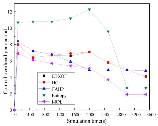
Figure 7. Control overhead.

4.3.2. Average Packet Delivery Ratio

Figure 8 shows the average packet delivery ratio of I-RPL, ETXOF, HC, FAHP, and entropy. It can be seen that, in the initial stage, the packet delivery ratio of each algorithm is unstable; it gradually reaches a stable state after 2000 s. And the average packet delivery ratio of I-RPL is obviously higher than that of ETXOF, HC, FAHP, and entropy, because I-RPL proposed using the recursive method to evaluate the REI and BOR of the candidate parent and comprehensively use the sum, mean and standard deviation of ETX and delay. The context-aware composite routing metric and C-OF are proposed. The scientific multiple routing metrics theories are designed. So, I-RPL can select the optimal path to deliver packets. Therefore, the packet delivery ratio of I-RPL is significantly better than that of other algorithms.

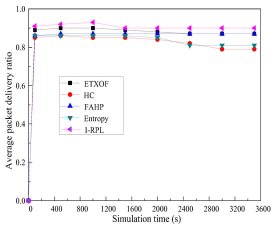
Figure 8. Average packet delivery ratio.

4.3.3. Average End-to-End Delay

Figure 9 shows the average end-to-end delay of I-RPL, ETXOF, HC, FAHP, and entropy. The end-to-end delay of I-RPL is obviously lower than that of other algorithms. I-RPL proposed new a network construction process to improve network construction efficiency. Moreover, the delay routing metric is evaluated in the manner of the sum, mean and standard deviation, etc. Therefore, the I-RPL can significantly improve end-to-end delay.

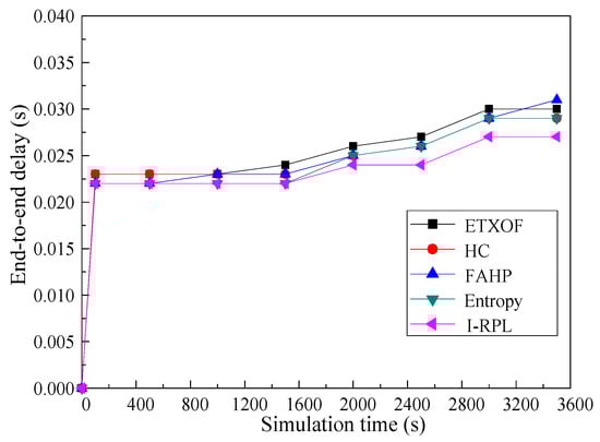
Figure 9. Average end-to-end delay.

4.3.4. Average Hop Count

Average hop count experiment results are shown in Figure 10. It is clear to see that I-RPL and HC are the minimum values. Since HC only selects the next hop based on the hop metric, the candidate parent with the minimum hop to destination will be selected as the preferred parent. The I-RPL can significantly reduce the hop count from source to destination based on the context-aware composite routing metric and C-OF, etc. Therefore, the hop count performance of I-RPL and HC are the best.

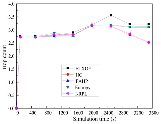
Figure 10. Average hop count.

4.3.5. Network Lifetime

Average remaining energy and average alive node number can estimate the network’s lifetime effectively. Figure 11 and Figure 12 show the I-RPL, ETXOF, HC, FAHP, and entropy of these two statistic metrics. It is clear to see that these two statistic metrics of I-RPL are much higher than that of ETXOF, HC, FAHP, and entropy. Since I-RPL reduces the control overhead by improving the DODAG build process—comprehensively evaluating REI, BOR, ETX, and D of the candidate parent—it designs scientific multiple routing metric evaluation theories. Therefore, I-RPL can significantly reduce energy consumption, save network resources, and prolong the network’s life.

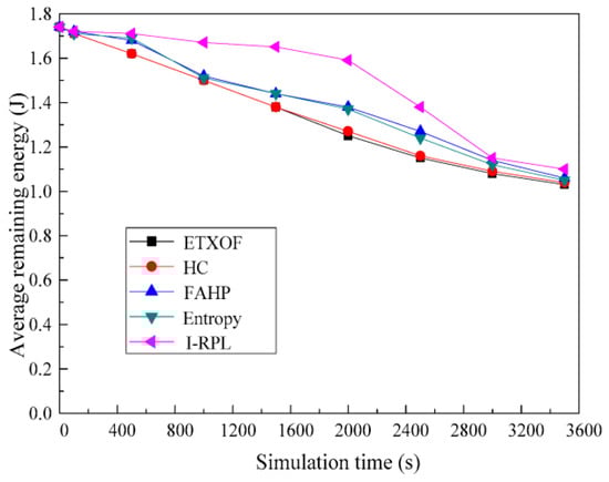
Figure 11. Average remaining energy.

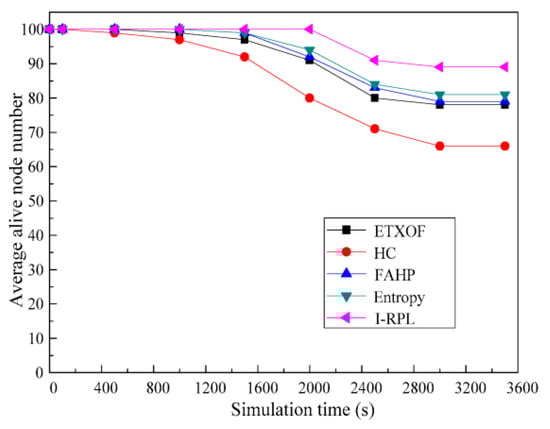
Figure 12. Average alive node number.

4.3.6. Average Number of Preferred Parent Changes

The average frequency of preferred parent changes is a reflection of the network topology stability, and it can be applied to coordinate network performance with the stability of the network topology. Figure 13 shows the average number of preferred parent changes in I-RPL, ETXOF, HC, FAHP, and entropy. It can be seen that, at the initial stage, the metric values of each algorithm are relatively large. After 2400 s, reaching the stable network state, the number of preferred parent changes in I-RPL are much lower than that of ETXOF, HC, FAHP, and entropy. Therefore, I-RPL can effectively improve network performance under the premise of ensuring network topology stability.

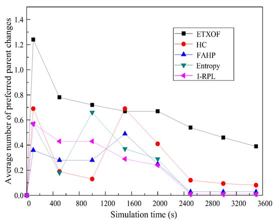
Figure 13. Average Number of Preferred Parent Changes.

4.3.7. Weight Coefficients (w₁, w₂, w₃, and w₄)

Figure 14 shows the relationship between weight factors (w₁, w₂, w₃, and w₄) and simulation time. In this paper, the variation law of the weight coefficient of node 6 (corresponding to (a)), node 38 (corresponding to (b)), node 54 (corresponding to (c)), and node 92 (corresponding to (d)) are randomly selected. It is obvious that the I-RPL can dynamically adjust values of w₁, w₂, w₃, and w₄ according to the network’s actual objective operation, users, control centers, and other subjective factors.

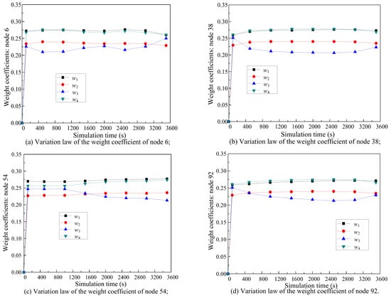
Figure 14. Relationship between weight factors (w₁, w₂, w₃, and w₄) and simulation time.

5. Conclusions

In this paper, I-RPL is proposed to better adapt to 6G LLN. I-RPL designed new context-aware routing metrics which evaluate the residual energy index, buffer occupancy ratio, ETX, delay, and hop comprehensively to guarantee multi-dimensional network QoS. Among them, the candidate parent and its preferred parent’s residual energy indicator and buffer utilization ratio are calculated recursively to reduce the effect of upstream parents. ETX and delay calculating manners are improved to ensure a better performance. Moreover, the I-RPL has optimized the network construction process, designed scientific multiple routing metric evaluation theories (Lagrangian multiplier theories), and proposed new rank computing and optimal route selecting mechanisms to improve network construction efficiency, energy consumption efficiency, broadcast suppression, network reliability, and so on. Finally, simulation experiments demonstrate that I-RPL is superior to other improvements.

In terms of future work, we plan to conduct more in-depth research into the 6G LLN routing algorithm and segment routing technology.

References

- Wang, C.X.; You, X.H.; Gao, X.Q.; Zhu, X.; Li, Z.; Zhang, C.; Wang, H.; Huang, Y.; Chen, Y.; Haas, H.; et al. On the Road to 6G: Visions, Requirements, Key Technologies, and Testbeds. IEEE Commun. Surv. Tutor. 2023, 25, 905–974. [Google Scholar] [CrossRef]
- Prajapati, A.K.; Pilli, E.S.; Battula, R.B.; Varadharajan, V.; Verma, A.; Joshi, R. A comprehensive survey on RPL routing-based attacks, defences and future directions in Internet of Things. Comput. Electr. Eng. 2025, 123, 110071. [Google Scholar] [CrossRef]
- Soyak, E.G.; Ercetin, O. Effective networking: Enabling effective communications towards 6G. Comput. Commun. 2024, 215, 1–8. [Google Scholar] [CrossRef]
- Yang, C.S.; Liao, Y.J.; Kuo, C.H.; Hwang, C.-H.; Wu, W.-D.; Liao, P.-K.; Fu, I.-K.; Sébire, G.; Frost, T.; Tenny, N. Toward 6G Sustainable Mobile Communications. IEEE Wirel. Commun. 2025, 32, 44–50. [Google Scholar] [CrossRef]
- Lakhlef, I.E.; Djamaa, B.; Senouci, M.R.; Bradai, A. Enhanced Multicast Protocol for Low-Power and Lossy IoT Networks. IEEE Sens. J. 2024, 24, 15393–15408. [Google Scholar] [CrossRef]
- Bono, F.M.; Polinelli, A.; Radicioni, L.; Benedetti, L.; Castelli-Dezza, F.; Cinquemani, S.; Belloli, M. Wireless Accelerometer Architecture for Bridge SHM: From Sensor Design to System Deployment. Future Internet 2025, 17, 29. [Google Scholar] [CrossRef]
- Parizi, M.N.; Ghafouri, S.H.; Hajmohammadi, M.S. TARRP: Trust Aware RPL Routing Protocol for IoT. Int. J. Commun. Syst. 2025, 38, e6124. [Google Scholar] [CrossRef]
- Dey, D.; Ghosh, N. iTRPL: An intelligent and trusted RPL protocol based on Multi-Agent Reinforcement Learning. Ad Hoc Netw. 2024, 163, 103586. [Google Scholar] [CrossRef]
- Zhu, X.Q.; Liu, J.Q.; Lu, L.Y.; Zhang, T.; Qiu, T.; Wang, C.; Liu, Y. Enabling Intelligent Connectivity: A Survey of Secure ISAC in 6G Networks. IEEE Commun. Surv. Tutor. 2025, 27, 748–781. [Google Scholar] [CrossRef]
- Lakhlef, I.E.; Djamaa, B.; Senouci, M.R.; Bradai, A.; Cherif, Y.M. PIM-LLN: Protocol Independent Multicast for Low-Power and Lossy Networks. IEEE Trans. Mob. Comput. 2025, 24, 3809–3825. [Google Scholar] [CrossRef]
- RFC9010; Thubert, P.; Richardson, M. Routing for RPL (Routing Protocol for Low-Power and Lossy Networks) Leaves. Internet Engineering Task Force (IETF): Fremont, CA, USA, 2021.
- RFC9008; Robles, M.I.; Richardson Thubert, P. Using RPI Option Type, Routing Header for Source Routes, and IPv6-in-IPv6 Encapsulation in the RPL Data Plane. Internet Engineering Task Force (IETF): Fremont, CA, USA, 2021.
- RFC6550; Winter, T.; Thubert, P.; Brandt, A.; Alexander, R.; Vasseur, J.P.; Hui, J.; Pister, K.; Levis, P.; Struik, R.; Kelsey, R. RPL: IPv6 Routing Protocol for Low-Power and Lossy Networks. Internet Engineering Task Force (IETF): Fremont, CA, USA, 2012.
- RFC8036; Winget, N.C.; Hui, J.; Popa, D. Applicability Statement for the Routing Protocol for Low-Power and Lossy Networks (RPL) in Advanced Metering Infrastructure (AMI) Networks. Internet Engineering Task Force (IETF): Fremont, CA, USA, 2017.
- Mohajerani, J.; Ghanatghestani, M.M.; Hashemipour, M. MCTE-RPL: A multi-context trust-based efficient RPL for IoT. Netw. Comput. Appl. 2024, 229, 103937. [Google Scholar] [CrossRef]
- Dinesh, P.S.; Palanisamy, C. Reliable Data Delivery and Load Balancing in Improved Energy Efficient RPL Routing Protocol for Low Power and Lossy Networks. Int. J. Commun. Syst. 2025, 38, e6106. [Google Scholar] [CrossRef]
- Vidhya, S.S.; Mathi, S.; Ananthanarayanan, V.; Iyer, G.N. IP-RPL: An Intelligent Power-Aware Routing Protocol for Next-Generation Low-Power Networks. IEEE Sens. J. 2025, 25, 3640–3648. [Google Scholar] [CrossRef]
- Hussain, S.J.; Roopa, M. BE-RPL: Balanced-load and Energy-efficient RPL. Comput. Syst. Sci. Eng. 2023, 45, 785–801. [Google Scholar] [CrossRef]
- Alilou, M.; Sangar, A.B.; Majidzadeh, K.; Masdari, M. QFS-RPL: Mobility and Energy Aware Multi Path Routing Protocol for The Internet of Mobile Things Data Transfer Infrastructures. Telecommun. Syst. 2024, 85, 289–312. [Google Scholar] [CrossRef]
- Ghosh, S. CB-ED-RPL: Coordinator-Based Energy-Efficient Dynamic RPL for IoT Networks. Wirel. Pers. Commun. 2023. [Google Scholar] [CrossRef]
- Rady, M.; Lampin, Q.; Barthel, D.; Watteyne, T. Bringing Life Out of Diversity: Boosting Network Lifetime Using Multi-PHY Routing in RPL. Trans. Emerg. Telecommun. Technol. 2022, 33, e4592. [Google Scholar] [CrossRef]
- Dharmalingaswamy, A.; Pitchai, L. Additive Metric Composition-Based Load Aware Reliable Routing Protocol for Improving the Quality of Service in Industrial Internet of Things. Int. Arab. J. Inf. Technol. 2023, 20, 954–964. [Google Scholar] [CrossRef]
- Vieira Junior, I.F.; Granjal, J.; Curado, M. RT-Ranked: Towards Network Resiliency by Anticipating Demand in TSCH/RPL Communication Environments. Netw. Syst. Manag. 2024, 32, 19. [Google Scholar] [CrossRef]
- Tabouche, A.; Djamaa, B.; Senouci, M.R.; Ouakaf, O.E.; Elaziz, A.G. TLR: Traffic-Aware Load-Balanced For Industrial IoT. Internet Things 2024, 25, 101093. [Google Scholar] [CrossRef]
- Maheshwari, A.; Panneerselvam, K. Optimizing RPL for Load Balancing and Congestion Mitigation in IoT Network. Wirel. Pers. Commun. 2024, 136, 1619–1636. [Google Scholar] [CrossRef]
- Royaee, Z.; Mirvaziri, H.; Bardsiri, A.K. Designing a context-aware model for RPL load balancing of low power and lossy networks in the internet of things. Ambient. Intell. Humaniz. Comput. 2020, 12, 2449–2468. [Google Scholar] [CrossRef]
- Pereira, H.; Moritz, G.L.; Souza, R.D.; Munaretto, A.; Fonseca, M. Increased Network Lifetime and Load Balancing Based on Network Interface Average Power Metric for RPL. IEEE Access 2020, 8, 48686–48696. [Google Scholar] [CrossRef]
- Kumar, A.; Hariharan, N. DCRL-RPL: Dual context-based routing and load balancing in RPL for IoT networks. IET Commun. 2020, 14, 1869–1882. [Google Scholar] [CrossRef]
- Hadaya, N.N.; Alabady, S.A. Proposed RPL routing protocol in the IoT applications. Concurr. Comput.-Pract. Exp. 2022, 34, e6805. [Google Scholar] [CrossRef]
- Alotaibi, M.A.; Alwakeel, S.S.; Alyahya, A.N. A Novel Reliable and Trust Objective Function for RPL-Based IoT Routing Protocol. CMC-Comput. Mater. Contin. 2025, 82, 3467–3497. [Google Scholar]
- Mishra, S.N.; Khatua, M. Reliable and Delay Efficient Multi-Path RPL for Mission Critical IoT Applications. IEEE Trans. Mob. Comput. 2024, 23, 6983–6996. [Google Scholar] [CrossRef]
- RFC9616; Jonglez, B.; Chroboczek, J. Delay-Based Metric Extension for the Babel Routing Protocol. Internet Engineering Task Force (IETF): Fremont, CA, USA, 2024.
- Behrad, B.V.; Abolfazl, T.H. Brad-OF: An Enhanced Energy-Aware Method for Parent Selection and Congestion Avoidance in RPL Protocol. Wirel. Pers. Commun. 2020, 114, 783–812. [Google Scholar] [CrossRef]
- Hanane, L.; Nabil, B. A comprehensive survey on enhancements and limitations of the RPL protocol: A focus on the objective function. Ad Hoc Netw. 2020, 96, 102001. [Google Scholar]
- Anita, C.S.; Sasikumar, R. Learning automata and lexical composition method for optimal and load balanced RPL routing in IoT. Int. J. Ad Hoc Ubiquitous Comput. 2022, 40, 288–300. [Google Scholar] [CrossRef]
- Kamble, S.; Chandavarkar, B.R. EWRPL: Entropy-based weighted RPL. Wirel. Netw. 2025, 31, 613–622. [Google Scholar] [CrossRef]
- Kamble, S.; Bhilwar, P.; Chandavarkar, B.R. Novel Fuzzy-based Objective Function for routing protocol for low power and lossy networks. Ad Hoc Netw. 2023, 144, 103150. [Google Scholar] [CrossRef]
- RFC6719; Gnawali, O.; Levis, P. The Minimum Rank with Hysteresis Objective Function. Internet Engineering Task Force (IETF): Fremont, CA, USA, 2012.
- Srisomboon, K.; Wasayangkool, K.; Lee, W. Trilateral Smart Switching Algorithm for Improving Smart Meters Efficiency in Advanced Metering Infrastructure (AMI) Network. IEEE Access 2024, 12, 194973–194988. [Google Scholar] [CrossRef]
- Shen, A.; Li, Y.; Noman, K.; Wang, D.; Peng, Z.; Feng, K. Multiscale fluctuation-based symbolic dynamic entropy: A novel entropy method for fault diagnosis of rotating machinery. Struct. Health Monit.-Int. J. 2025, 24, 402–420. [Google Scholar] [CrossRef]
- Xiong, Z.C.; Hu, J.Y.; Li, N. Comprehensive quality evaluation method of ultrasound tomography algorithms based on entropy method. Meas. Sci. Technol. 2024, 35, 115403. [Google Scholar] [CrossRef]
- Cao, Y.N.; Yuan, H. A novel context-aware RPL algorithm based on a triangle module operator. Front. Inf. Technol. Electron. Eng. 2021, 22, 1583–1597. [Google Scholar] [CrossRef]
Disclaimer/Publisher’s Note: The statements, opinions and data contained in all publications are solely those of the individual author(s) and contributor(s) and not of MDPI and/or the editor(s). MDPI and/or the editor(s) disclaim responsibility for any injury to people or property resulting from any ideas, methods, instructions or products referred to in the content. |
© 2025 by the authors. Licensee MDPI, Basel, Switzerland. This article is an open access article distributed under the terms and conditions of the Creative Commons Attribution (CC BY) license (https://creativecommons.org/licenses/by/4.0/).