Abstract
The widespread application of wireless communication has led to increasingly complex electromagnetic environments, where spectrum abuse and malicious interference frequently cause abnormal signals. Radio anomaly detection technology has emerged to address these challenges. This paper focuses on the performance limitations of existing radio anomaly detection methods under low interference-to-signal ratio (ISR)conditions. We propose a fusion detection algorithm, LOF-OCSVM, integrating local outlier factor (LOF) and one-class support vector machine (OCSVM). Innovatively, we introduce three novel features: fluctuation entropy (FE), fluctuation mutual information (FR-MI), and lognormal distribution fitting parameters derived from signal fluctuation sequences. These features quantify the disorderliness, adjacent correlation, and statistical distribution characteristics of signal fluctuations, significantly enhancing the detection sensitivity for weak interference signals. Simulation experiments demonstrate that: feature effectiveness: the new features improve recall by >30% and F1-score by >23% at −20 dB ISR. Model superiority: the LOF-OCSVM fusion model achieves an F1-score of 0.8634 at −20 dB ISR through a hierarchical decision mechanism, outperforming single model and simple hybrid approaches. Robustness: compared to Deep SVDD and E-GAN, our method improves AUC by 3% under low ISR conditions while maintaining stronger robustness.
1. Introduction
The rapid advancement of wireless communication technology has brought benefits and convenience to people’s production and daily lives, while also imposing higher requirements on the security design of communication systems. At the same time, the limited spectrum resources and the widespread application of wireless communications have made spectrum conflicts increasingly prominent, with issues such as co-channel interference and unauthorized signal intrusion occurring frequently. Additionally, the inherently open nature of radio signals makes them susceptible to attacks such as eavesdropping, jamming, interception, and even spoofing during transmission, undoubtedly posing more severe challenges to spectrum management and wireless communication security.
Current research on radio security primarily focuses on two categories: spectrum monitoring technologies and interference detection and identification technologies. Among these, spectrum monitoring technologies can be further subdivided based on task emphasis into spectrum sensing technologies, cognitive radio technologies, modulated signal recognition technologies, and radio anomaly detection technologies. Radio anomaly detection technology can quickly identify intrusion signals and abnormal signals, providing a powerful technical means for wireless communication security detection. To address the issue of low detection performance under low interference-to-signal ratio (ISR) in current anomaly detection research, this paper proposes an anomaly detection method that combines three features, namely fluctuation entropy (FE), fluctuation mutual information (FR-MI), and the lognormal distribution fitting coefficient of fluctuation sequences—with an ensemble learning model based on local outlier factor (LOF) and one-class support vector machine (OCSVM). This approach significantly improves detection performance under low ISR conditions.
2. Related Works
Currently, radio anomaly detection technologies can be broadly categorized, based on the methods used, into traditional detection methods, evolutionary algorithm-based detection methods, and machine learning-based detection methods. The specific methods are summarized in Figure 1.
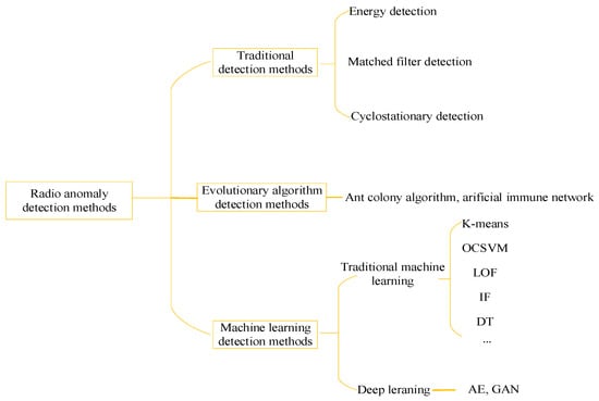
Figure 1.
Radio Anomaly Detection Methods.
Traditional detection methods primarily include energy-based detection, matched filter detection, and cyclostationary feature-based detection. Urkowitz [1] first proposed the use of energy detection for identifying unknown deterministic signals by measuring the energy of the input wave over a specific time interval to determine the presence of a signal. Subsequently, scholars proposed frequency-domain energy detection methods, which can not only determine the presence of interference signals but also obtain characteristic parameters such as frequency and energy of the interfering signals. Henttu et al. [2] first proposed the consecutive mean excision (CME) algorithm, which iteratively calculates the current energy mean to derive a dynamic threshold and removes abnormal signals exceeding this threshold to achieve anomaly detection. Saarnisaari et al. [3] introduced the forward consecutive mean excision (FCME) algorithm, which uses forward verification of the minimum energy set to detect signal anomalies even under high pollution ratios. Reference [4] proposed an iterative energy-aware algorithm for adaptive threshold adjustment and virtual alarm elimination based on the AND criterion. Reference [5] categorized signal anomalies into three types: anomalies caused by malicious high-power interference, unauthorized signals, and authorized signals violating frequency usage regulations. For malicious interference signals, it proposed a method using relative wavelet time entropy as a feature parameter to characterize the signal’s energy level attributes for detecting malicious interference. Masari et al. [6] analyzed and compared the application of static and dynamic thresholds in two traditional spectrum sensing methods: energy detection and matched filter detection. Experiments demonstrated that for energy detection, static thresholds perform better under low signal-to-noise ratio (SNR) conditions, while dynamic thresholds excel in high SNR environments. For matched filter detection, dynamic thresholds provide higher detection rates across most SNR conditions. Liang [7] and Zhang [8] improved the FCME algorithm to detect interference in civilian BeiDou signals. Literature [9] addressed the issue of blocking interference in railway wireless communications by proposing an automatic identification method based on adaptive chirp mode decomposition and spectrum sensing, utilizing real-time dynamic spectrum detection data. Energy detection methods, which require no prior knowledge of the interfering signal and only use signal energy characteristics for threshold-based anomaly detection, offer the advantages of simple computation and ease of implementation. They are also the most widely used detection methods. However, these methods also have drawbacks, such as high requirements for SNR and susceptibility to missed detections under low ISRs. Matched filter detection is a coherent detection method that correlates the received signal with a known primary user signal or desired signal to detect the primary user signal. It detects anomalies by observing output peaks. Such methods often assume complete knowledge of the signal’s characteristic parameters, requiring extensive prior information about the signal. Consequently, their application scenarios are relatively limited. Cyclostationary feature-based detection methods leverage the inherent periodicity of modulated signals to distinguish between signals, noise, and interference. They extract and identify feature peaks by calculating the spectral correlation function, thereby detecting signal anomalies. These methods maintain certain advantages even at low SNRs but suffer from high computational complexity, which hinders their practical engineering implementation.
Evolutionary algorithm-based detection methods identify various anomalous signals by transforming the anomaly detection problem into a path optimization challenge. For instance, Xiong et al. [10] proposed an improved ant colony algorithm based on 20 features—including signal strength, channel state, and carrier frequency—for the automatic identification of anomalous signals in wireless communication networks. By incorporating multi-colony collaboration, dynamic pheromone updating, and heuristic weight enhancement, the algorithm’s performance in identifying anomalous signals was significantly improved. Additionally, some researchers have applied artificial immune systems [11,12,13] to develop immune network-based models for monitoring abnormal electromagnetic signals. These models introduce the “self-nonself” discrimination mechanism from artificial immune systems, treating background signals as “self” and abnormal signals as “nonself” to detect electromagnetic anomalies. However, these methods suffer from high computational complexity and rely on pure background signals during the training phase, making them difficult to apply effectively in proposed battlefield environments and complex electromagnetic scenarios.
With the continuous development of machine learning and artificial intelligence algorithms, an increasing number of researchers have leveraged machine learning or deep learning algorithms to achieve effective detection of anomalous radio signals, yielding promising results. Feng [14], Yu et al. [15], and Pang et al. [16] combined improved Support Vector Machine (SVM) algorithms to detect anomalous spectrum signals. Qi [17] proposed an improved clustering algorithm based on a combination of Chameleon and K-means for anomaly detection. This approach first divides frequency band slices into small signal clusters, and then extracts features such as frequency, bandwidth, and amplitude within each cluster to compare with existing signal data in a database for anomaly detection. Feng [18] addressed deceptive intrusion signals by utilizing signal fluctuation characteristics for detection. The method involves calculating the fluctuation amplitude between two consecutive frames to form a fluctuation sequence, then computing the probability mass functions for both legitimate and test signals. By incorporating Kullback–Leibler divergence, intrusion detection is achieved. To tackle the issue of low-power intrusion signals being filtered out during noise elimination, a power entropy-based intrusion detection algorithm was proposed. This technique analyzes the time-frequency power graph of the target frequency band to derive power value sequences for each frequency point, subsequently obtaining their probability mass functions and power entropy. An OCSVM is trained using power entropy curves from normal states to detect low-power intrusion signals. Wang [19] extracted features from the time domain, frequency domain, and time-frequency domain, including time-domain moment skewness, spectral kurtosis, carrier factor, 0.5-times bandwidth, and maximum value in the fractional Fourier domain. These features were used with both Decision Tree (DT) and SVM algorithms to achieve interference detection. Yengi et al. [20] addressed three typical attacks in LTE-A relay security—jamming, regeneration, and false data injection attacks—by constructing feature vectors based on baseband signal amplitude, phase, and relative phase for anomaly detection. They compared the detection performance of three algorithms—LOF, OCSVM, and Isolation Forest (IF)—under different SNRs and modulation schemes. Among them, LOF demonstrated the best overall performance in attack detection, OCSVM performed better in resource-constrained scenarios, while IF was more suitable for high-resource environments. Hong et al. [21] proposed a hybrid machine learning algorithm based on DT and IF to identify known interference attacks and detect unknown attacks. For each leaf node of the DT, an IF model was trained separately. During the classification and detection process, the corresponding IF model was selected based on the DT classification result for anomaly determination. If the result was normal, the DT classification was accepted; if anomalous, it was considered an unknown attack. Experiments conducted on self-collected C-band datasets and public datasets showed that this approach outperformed baseline methods. In addition to these conventional machine learning methods, Ford et al. [22] proposed a machine learning approach based on switching linear dynamical systems. They used Bayesian nonparametric hierarchical Dirichlet process techniques to train switching linear dynamical systems to represent interference and noise environments. A generalized likelihood ratio test was employed to determine whether the Viterbi hidden switching state path of the test data was sufficiently improbable under the learned system, thereby detecting the presence of unknown signals. In recent years, advancements in artificial intelligence, particularly in deep learning algorithms, have brought transformative changes to various fields. In the domain of radio anomaly detection, researchers often use reconstruction error to identify anomalies. Rajendran et al. [23] proposed an adversarial autoencoder-based wireless spectrum anomaly detector, termed SAIFE. They used a Long Short-Term Memory (LSTM) network as the encoder to output two types of latent variables: explainable features and categories, and a Convolutional Neural Network (CNN) as the decoder. Two discriminators for features and categories were introduced, and three anomaly scores—reconstruction error, discrimination loss, and classification error—were computed. If any score exceeded a threshold, the signal was identified as anomalous. The discriminator results were further analyzed to determine the type of anomaly, such as unknown signal patterns or cross-band interference. Reference [24] still uses CNN for modulation recognition and interference recognition. Zhou et al. [25] proposed a radio signal anomaly detection algorithm based on an improved Generative Adversarial Network (GAN). Signals were converted into spectrograms via Short-Time Fourier Transform (STFT), and a novel encoder structure, E-GAN, was introduced by integrating an encoder network into the original GAN to reconstruct the spectrograms. Anomalies were detected based on a weighted anomaly score combining reconstruction error and discriminator loss. Compared to the SAIFE algorithm proposed in reference [23], this method achieved a performance improvement of 10 dB. References [26,27,28] employs improved GAN and Autoencoder to detect radio anomalies by learning the distribution of normal signals and their power spectral density. Compared to traditional detection methods and evolutionary algorithms, machine learning-based radio signal anomaly detection does not rely heavily on domain-specific knowledge and offers rapid and efficient detection capabilities. However, deep learning algorithms, due to their deeper network architectures, often require more memory resources and computational overhead. Additionally, the black-box nature of neural networks typically provides only detection results, posing challenges in interpretability. Therefore, this paper primarily employs unsupervised machine learning algorithms such as LOF and OCSVM to investigate radio anomaly detection techniques. The main contributions of this paper are as follows:
- (1)
- To address the current challenge of poor radio anomaly detection performance under low ISRs, this paper proposes features based on signal fluctuation sequences, including fluctuation entropy (FE), fluctuation mutual information (FR-MI), and the lognormal distribution coefficient derived from fitting fluctuation sequences. By incorporating these fluctuation-based features alongside commonly used features, the detection performance under low ISRs is significantly enhanced.
- (2)
- To overcome the difficulty of balancing detection rate and false alarm rate with a single model, an ensemble learning algorithm named LOF-OCSVM is proposed, which integrates the LOF and OCSVM algorithms. The OCSVM algorithm constructs a global decision boundary in a high-dimensional feature space to distinguish normal data from anomalies, while the LOF algorithm identifies anomalies by comparing the local density deviation of a data point relative to its neighbors. LOF is sensitive to local density variations and does not require assumptions about global data distribution. By combining these two algorithms, the proposed method significantly improves the detection performance for both global and local anomalies.
- (3)
- Referring to the methodology in reference [18], simulated signals were generated and experiments were conducted on a simulated dataset. The results demonstrate that the proposed method exhibits outstanding overall performance and strong robustness, particularly under low ISRs. The F1-score improved by approximately 1 percentage point compared to the typical deep anomaly detection algorithm Deep SVDD at −20 dB ISR, and by approximately 5 percentage points compared to the innovative E-GAN algorithm proposed in the literature [18].
3. Fluctuation Sequence Features
In the research of radio anomaly detection technology, feature extraction is a core step for distinguishing between normal and abnormal signals. It requires careful design and extraction based on the time-frequency domain characteristics, statistical properties, and physical attributes of signals. Commonly used features include: Time-domain features: mean, variance/standard deviation, peak/valley values, kurtosis, skewness, zero-crossing rate, etc. Frequency-domain features: center frequency, bandwidth, spectral entropy, peak frequency, spectral flatness, etc. Time-frequency domain features obtained through transformations such as STFT, such as time-frequency center which reflects the centroid coordinates of energy on the time-frequency plane and time-frequency bandwidth which reflects the distribution range of signals on the time-frequency plane. Energy-domain features: signal power, energy entropy, power spectral density, power change rate, etc. Under high ISRs, abnormal signals significantly deviate from normal signals, allowing the above features to achieve satisfactory detection performance. However, in cases of weak signal perturbations with low ISRs, these features exhibit broad monitoring ranges and strong statistical properties, leading to coarse detection that struggles to capture subtle changes in radio spectrum anomalies. Given the inherent fluctuating nature of wireless communication, take amplitude-modulated signals as an example, whose formula is as follows:
Among them, represents the amplitude of the carrier wave, is the modulation index, denotes the baseband signal, and represents the carrier frequency. As evident from the formula, the amplitude of the signal is a function of time, meaning the signal strength is inherently time-varying. Additionally, factors such as environmental interference, noise, and power fluctuations of the signal transmitter can also cause fluctuations in the received signal strength. In other words, the strength of the received signal is closely related to the transmitting equipment, noise environment, interference, and other factors. Under different operating conditions, the fluctuation characteristics of signals vary. To leverage this property, this paper proposes three features related to signal fluctuation characteristics for radio signal anomaly detection. These features are: fluctuation entropy, fluctuation mutual information, and the shape and location parameters obtained by fitting the signal fluctuation characteristics to a lognormal distribution.
3.1. Fluctuation Entropy
In wireless communications, normal signals typically exhibit stable modulation patterns and time-frequency structures. Their variations in the time dimension, such as fluctuations in amplitude and frequency, demonstrate strong regularity. In contrast, abnormal signals—such as those distorted by malicious interference or equipment failures—disrupt this regularity, leading to disordered fluctuation patterns in the time-frequency domain. Therefore, this paper proposes the FE feature to quantify the uncertainty of fluctuation amplitude sequences in the time-frequency domain. The core input for calculating fluctuation entropy is the fluctuation amplitude sequence, which reflects the degree of variation between adjacent frames of the signal in the time-frequency domain. Assuming the spectrogram obtained after STFT is represented as follows:
where represents the number of time frames and denotes the number of frequency points. The fluctuation amplitude value is defined as:
where represents the magnitude value at time frame and frequency bin. By iterating through all adjacent frames, the fluctuation amplitude sequence is obtained as .
The calculation of fluctuation entropy is based on the fluctuation amplitude sequence and Shannon entropy theory. It involves discretization through binning operations and probability distribution modeling to compute the entropy value. The specific calculation steps are as follows:
Step 1: Sequence discretization, the fluctuation amplitude sequence is divided into B equal-width intervals. The range of these intervals is determined by the minimum and maximum values of the sequence, namely .
Step 2: Probability distribution Estimation, the number of samples falling into each interval is counted, and the probability distribution is derived, where , represents the number of samples in interval, and .
Step 3: Entropy calculation, the fluctuation entropy is defined as the Shannon entropy of this probability distribution, calculated as follows:
where is an extremely small value introduced to prevent .
The proposed fluctuation entropy feature primarily serves to capture the dynamic variation patterns of signals across adjacent time periods, rather than focusing on static amplitude or power values. By quantifying the uncertainty within the fluctuation amplitude sequence—that is, the degree of disorder in its variations—this feature can more sensitively reflect disturbances caused by anomalous interference, thereby enabling the detection of radio abnormalities.
3.2. Fluctuation Mutual Information
The fluctuation entropy feature quantifies the overall uncertainty of the signal fluctuation amplitude sequence but does not capture the dynamic correlations within the sequence—specifically, the dependency relationships between adjacent fluctuations. In wireless communications, normal signals exhibit not only stable fluctuation patterns and low information entropy but also continuity in fluctuations across adjacent time intervals. In contrast, abnormal signals caused by factors such as burst interference disrupt this continuity, leading to a significant decline in the correlation between adjacent fluctuations. To address this, this paper proposes the FR-MI feature to quantify the statistical dependency between adjacent elements in the fluctuation amplitude sequence. This feature focuses on the “temporal continuity” of fluctuation patterns, complementing fluctuation entropy to collectively capture the “disorder” and “correlation disruption” introduced by abnormal signals.
Based on the fluctuation amplitude sequence defined in the context of fluctuation entropy, adjacent element pairs are extracted. For the fluctuation amplitude sequence , where , each pair reflects the correlation between the fluctuation and the fluctuation.
The calculation of fluctuation mutual information primarily quantifies correlations based on joint probability distributions and enhances interpretability through normalization. The calculation procedure consists of the following steps:
Step 1: Two-dimensional discretization, the set of fluctuation pairs is mapped onto a B × B two-dimensional grid. The grid range is still determined by the minimum and maximum values of the original sequence .
Step 2: Joint probability distribution, count the number of fluctuation pairs falling into each grid cell to obtain a joint frequency distribution namely , which is then normalized as .
Step 3: Marginal probability distribution estimation. The marginal probability distributions are obtained as and by summing the joint distribution along each of the two dimensions.
Step 4: Mutual information calculation. The original mutual information is computed based on the Shannon mutual information formula, expressed as:
where is introduced to prevent the denominator from being zero.
Step 5: Normalization, the original mutual information is normalized by dividing it by the maximum possible mutual information , resulting in the fluctuation mutual information with a value range of [0, 1]. The formula is as follows:
where the maximum possible mutual information is denoted as , because the calculation of mutual information is constrained by the entropy of the variables and has a theoretical upper bound. Its value range is , where and represent the entropy of variables and , respectively. In the context of fluctuation mutual information, variables and correspond to two adjacent fluctuation pairs from the same fluctuation amplitude sequence. Therefore, , since we perform binning operations on the fluctuation amplitude sequence, the values of each variable are discretized into B possible states. According to information theory, the maximum entropy of a discrete variable is . That is, when the variable is uniformly distributed across B states, the uncertainty is maximized. Therefore, the theoretical upper bound of mutual information is constrained by the maximum entropy of the variables, namely . In practical computation, the calculation of fluctuation mutual information also relies on estimation based on a limited number of fluctuation pair samples N. According to sampling theory, the maximum amount of information that can be provided by a finite sample set cannot exceed Therefore, the maximum possible mutual information must simultaneously satisfy both the theoretical upper bound determined by the number of bins B and the practical upper bound constrained by the sample size N. Taking the minimum of these two values , as the normalization denominator ensures that the normalized fluctuation mutual information , avoids exceeding the upper limit due to insufficient samples or excessive binning.
After normalization, an FR-MI value closer to 1 indicates stronger correlation between adjacent fluctuations, while a value closer to 0 suggests weaker correlation and higher disorder.
The FE feature measures the overall disorder of fluctuations, while the FR-MI feature quantifies the local continuity of fluctuations. Two sequences with identical FE values may be effectively distinguished by FR-MI due to differences in the correlation between adjacent fluctuations. This means the FR-MI feature enhances sensitivity to transient anomalies beyond what the FE feature alone can capture. For instance, anomalous interference that causes abrupt changes in the fluctuation sequence and significantly reduces the correlation between adjacent fluctuations may lead to a sharp drop in the FR-MI value, which might not be detected solely by Fluctuation Entropy. Therefore, the FR-MI feature serves as an effective complement to the FE feature.
3.3. Lognormal Distribution Fitting Parameters
While FE and FR-MI, respectively, characterize the disorder and adjacent correlations of the fluctuation amplitude sequence, they do not directly describe the statistical distribution characteristics of the sequence. In radio signals, the fluctuation amplitudes of normal signals typically exhibit a right-skewed distribution dominated by small fluctuations with rare large-amplitude variations. As previously analyzed, the values in the fluctuation amplitude sequence are all non-negative and may contain a few extreme large values. However, anomalous signals often distort the fluctuation sequence, altering this distribution pattern. Therefore, this paper proposes a feature based on lognormal distribution fitting parameters. By extracting the shape and scale parameters of the lognormal distribution fitted to the fluctuation amplitude sequence, this feature quantifies the overall statistical distribution pattern of the sequence, serving as supplementary evidence for anomaly detection.
For a random variable (representing the fluctuation amplitude value), if its natural logarithm follows a normal distribution , then follows a lognormal distribution, with its probability density function given by:
where is the log-mean namely location parameter, which determines the central tendency of the distribution; and is the log-standard deviation namely shape parameter, which determines the dispersion and skewness of the distribution. In practical applications, we primarily focus on , the shape parameter reflecting the dispersion of fluctuation amplitudes and , the scale parameter reflecting the typical level of fluctuation amplitudes. For the fluctuation amplitude sequence , the parameter estimation procedure is as follows:
Step 1: Data preprocessing. Take the natural logarithm of each element in the sequence to obtain: .
Step 2: Normal distribution fitting. Use Maximum Likelihood Estimation (MLE) for to fit a normal distribution to , obtaining the log-mean and log-standard deviation as follows:
Step 3: Feature parameter extraction. The final features are the shape parameter and the scale parameter , where is the geometric mean of the original fluctuation amplitude sequence. This scale parameter quantifies the typical level of fluctuation amplitudes—a higher value indicates more intense overall fluctuations.
4. Fusion Model
Due to the differences in the underlying mathematical principles of anomaly detection models, a single detection model often has different detection emphases, leading to certain limitations. For example, LOF excels at capturing local density deviation anomalies but tends to overlook global anomalies, while OCSVM performs well in high-dimensional feature spaces and is sensitive to global anomalies but lacks sufficient sensitivity to local outliers. To address this, this paper proposes an ensemble model that integrates LOF and OCSVM, leveraging their complementary strengths to enhance detection robustness and stability across various ISR scenarios, particularly under low ISR conditions.
4.1. Introduction to Base Models
LOF is a density-based anomaly detection algorithm. Its core idea is to identify anomalies by comparing the density discrepancy between a sample and its local neighborhood. The algorithm is as follows:
Step 1: Set the parameter k representing number of neighbors.
Step 2: Calculate the k-distance for sample p. For each sample, compute its distance to the k-th nearest neighbor, denoted as . Define the k-distance neighborhood as the set of all points o whose distance to p does not exceed .
Step 3: Calculate the reachability distance: The reachability distance from point p to a neighboring point o is defined as:
where sample o is a neighbor of the sample p under evaluation, and represents the distance from o to its own k-th nearest neighbor.
Step 4: Compute the Local Reachability Density (LRD):
Here, the denominator represents the sum of reachability distances from p to all its neighbors, and the numerator is the number of neighbors. LRD essentially measures the number of neighbors per unit reachability distance, reflecting the local density—a higher value indicates greater density.
Step 5: Calculate the Local Outlier Factor (LOF):
The criterion for judgment is as follows: if LOF ≈ 1, it indicates that the sample p under evaluation has a density comparable to its neighbors and is classified as a normal sample. If LOF > 1, it suggests that p has a lower density than its neighbors and is likely an anomalous sample, with a higher LOF value indicating a greater probability of being an anomaly.
OCSVM is an unsupervised algorithm designed to learn a decision boundary such that data points within the boundary are considered normal, while those outside are treated as anomalies. Its core idea involves mapping data to a high-dimensional feature space and finding a maximum-margin hyperplane that separates the data points from the origin as effectively as possible.
Given training data , the optimization problem for OCSVM is formulated as follows:
where is the normal vector of the hyperplane, is the distance from the hyperplane to the origin (i.e., the offset), and the decision boundary is defined as , represents slack variables that allow some data points to lie outside the boundary, controls the upper bound on the proportion of outliers and the proportion of support vectors, and is a nonlinear mapping that projects the data into a high-dimensional feature space.
Introducing Lagrange multipliers and
Introducing the KKT conditions for variable elimination: Let we obtain:
Substituting into L to eliminate , , , the dual problem of the optimization formulation is obtained as:
where is the kernel function, representing the value computed between sample points and . It essentially measures the similarity between two samples in the high-dimensional feature space. is a nonlinear mapping function that transforms the original input data from a low-dimensional space to a high-dimensional feature space to address linearly inseparable problems. <•,•> denotes the dot product operation in the high-dimensional space. This project employs the Gaussian (RBF) kernel:
The decision function after training is:
where an output of +1 indicates a normal sample within the decision boundary, while −1 represents an anomalous sample outside the boundary. The parameter denotes the bandwidth of the RBF kernel, controlling the influence range of individual samples.
4.2. Fusion Model Design and Implementation
The proposed integrated model is built upon two pre-trained models, LOF and OCSVM, with a core workflow consisting of “feature extraction, individual model scoring, weighted fusion, hierarchical decision-making”. The overall detection process is illustrated in Figure 2.
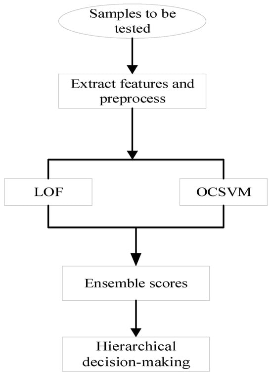
Figure 2.
Integrated Model Detection Process.
Step 1: Extract physical features from the spectrogram of the sample to be tested. Standardize the features using the mean and standard deviation of the training set, then input them into both pre-trained base models: LOF and OCSVM.
Step 2: Generate and standardize base model scores. The LOF and OCSVM models output raw anomaly scores and , respectively. To eliminate scale differences, standardize these raw scores based on the score distribution of normal samples in the training set.
Step 3: Perform weighted fusion of the standardized anomaly scores from the two models to generate an integrated score.
where and represent the weights assigned to the LOF model and OCSVM model, respectively, satisfying + = 1.
Step 4: Based on the integrated score, base model scores, and adaptive thresholds, the final label and confidence level of the test sample are determined through hierarchical decision-making.
To enhance detection reliability, the integrated model incorporates a hierarchical decision mechanism comprising preliminary prediction and low-confidence correction. It replaces manual threshold settings with adaptive thresholds to improve scenario adaptability. All adaptive thresholds are calculated based on the score distribution of normal samples in the training set, including the base model thresholds , , and the integrated score threshold . The kernel density estimation method is employed to fit the score distributions of normal training samples from the base models and the integrated score distribution after weighted fusion, respectively. The critical values corresponding to the prior proportion of normal samples are then taken as the thresholds, namely . Where denotes the anomaly sample ratio set during the training of the base models.
Hierarchical decision-making:
Step 1: Using the integrated score as the core criterion, if , the sample is preliminarily classified as anomalous; Otherwise, it is classified as normal.
Step 2: Correction for low-confidence samples, low-confidence samples with integrated scores close to the threshold are identified. If the integrated score of a test sample satisfies the condition: , where is a predefined hyperparameter for low-confidence tolerance, the sample is flagged as low-confidence. The following correction rules are applied: Calculate the confidence levels of the two base models: , . If both models exhibit high confidence and yield consistent predictions, adopt the consistent result. If the confidence levels differ significantly , where is a hyperparameter for significant difference threshold, adopt the result from the model with higher confidence as the final detection outcome. The pseudocode for the fusion algorithm is shown in Algorithm 1:
| Algorithm 1 LOF-OCSVM anomaly detection fusion algorithm |
| Input: spectrogram sample , pre-trained based models and , feature normalizer , thresholds , fusion weight , base model difference threshold Output: predicted label |
| 1: feature extraction and normalization: 2: base model scoring and standardization: , 3: weighted fusion: 4: hierarchical decision-making: 5: if : 6: y = 1 7: else: 8: y = 0 9: end if 10: low-confidence correction: 11: if : 12: 13: if >: 14: if >0: 15: 16: else 17: 18: end if 19: end if 20: end if |
5. Experimental Results and Analysis
5.1. Experimental Environment and Dataset
All experiments were executed and processed on a high-performance server with the following hardware configuration: a 16-core Intel Xeon Gold 6430 CPU (Intel Corporation; Santa Clara, CA, USA) and an NVIDIA RTX 4090 GPU(NVIDIA Corporation; Santa Clara, CA, USA) with 24 GB of dedicated memory, running on the Ubuntu 22.04 operating system. Additionally, during the experimental process, the hyperparameters related to the LOF-OCSVM fusion algorithm were configured as follows: the weights for LOF and OCSVM were set to 0.8 and 0.2, respectively; the low-confidence interval parameter was set to 0.08; and the model difference threshold was set to 0.5. These values were determined through a traversal method with a step size of 0.01 within their corresponding value ranges. For the model score threshold, since the training phase consisted entirely of normal samples, the 99th percentile of the kernel density estimation was selected based on empirical experience as the adaptive threshold. The contamination ratio for both base models during training was also set to 0.01, and the number of LOF neighborhoods was set to 20.
Following the methodology of reference [18], this paper simulates and generates an OFDM wireless communication signal dataset, including normal signals and four types of anomalous signals: single-tone interference, pulse interference, chirp interference, and unauthorized interference. The key parameters are highly consistent with those in reference [18]: the simulated spectrum consists of 6 channels, with offset frequencies relative to the center frequency of the simulated frequency band set at −50 MHz, −30 MHz, −10 MHz, 10 MHz, 30 MHz, and 50 MHz, respectively, resulting in a total bandwidth of 120 MHz. Each channel transmits an OFDM signal with 1200 subcarriers, a subcarrier spacing of 15 kHz, and uses QPSK as the modulation scheme. The simulated signal band operates in a symbol-level frequency-hopping dynamic mode, meaning one OFDM signal persistently exists in channel 3, while another OFDM signal randomly hops among channels 2, 5, and 6. The STFT parameters are set as follows: window length 256, overlap length 192, number of points 512, and sampling rate 120 × 106.
The dataset comprises 10,896 samples, divided into training and test sets. The training set contains 8096 normal signal samples. The test set includes 1000 normal signal samples and 1800 anomalous signal samples. The anomalous signals are superimposed on normal signals at specified ISR values, ranging from −20 dB to 20 dB in 5 dB increments. For each ISR value, there are 50 samples per anomaly type, resulting in 200 anomalous samples per ISR level. When evaluating model performance under different ISR conditions, the corresponding test set is constructed using 1000 normal signals and 200 anomalous signals. Each sample is converted into a time-frequency representation via STFT, ultimately generating a compressed spectrogram of size 64 × 64. We visualized the time-frequency diagrams of normal signals and anomalous signals at 0 dB ISR, with the results shown in Figure 3.
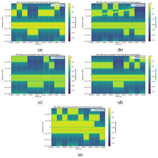
Figure 3.
Time-Frequency Diagrams of Different Signal Samples: (a) Normal signal sample; (b) Chirp interference signal sample; (c) Pulse interference signal sample; (d) Tone interference signal sample; (e) Unauthorized interference signal sample.
5.2. Feature Effectives Validation
We first extracted the fluctuation amplitude sequences from the normal samples in the training set of the simulated dataset. These sequences were used to plot: the distribution histogram of the sample fluctuation amplitudes, the distribution histogram after logarithmic transformation and the fitted normal distribution curve Additionally, two core visualization tools from statistics were employed to validate the data distribution morphology: Quantile-Quantile (Q-Q) plot and cumulative distribution function (CDF) plot. These tools were applied through quantile matching and cumulative probability curves to verify and visualize the distribution morphology of the fluctuation amplitude sequence data, thereby determining whether the data conforms to a lognormal distribution. The results are shown in Figure 4.
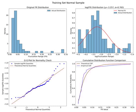
Figure 4.
Visualization of Fluctuation Amplitude Sequence Distribution.
Analyzing the subplot of the original fluctuation range (FR) distribution in the upper-left corner of Figure 4, it can be observed that the original FR exhibits a distinct right-skewed characteristic, with the peak concentrated on the left side where FR values are smaller, while the right interval with larger FR values shows a long-tail phenomenon. These features align with the “right-skewed and non-negative” properties of a lognormal distribution. Furthermore, the histogram of the logarithmically transformed data reveals an approximately bell-shaped distribution, with its trend largely consistent with the fitted normal curve. The Q-Q plot indicates that the blue scatter points generally adhere closely to the red reference line, suggesting that the quantiles of the logarithmically transformed fluctuation amplitude sequence approximately match those of the theoretical normal distribution. Similarly, the CDF plot demonstrates that the theoretical CDF based on the normal distribution fitted to log(FR) aligns well with the empirical CDF calculated from the original FR data, indicating overall consistency between the actual and theoretical distributions. Based on the above analysis, we propose using the lognormal distribution to model the fluctuation amplitude sequence and extract its fitted parameters as new features for anomaly detection.
To validate the effectiveness of the three types of features proposed in this paper for radio anomaly detection, we conducted feature ablation experiments. Using nine commonly adopted features in radio spectrum anomaly detection techniques: spectral centroid, bandwidth, total power, spectral flatness, power variance, peak factor, kurtosis, frequency change rate, and power entropy as the baseline, we performed the following: single-feature effectiveness experiments: individually incorporating each of the proposed features: FE, FR-MI, and the lognormal distribution fitting parameters of the fluctuation sequence—into the baseline feature set. Overall feature effectiveness experiment: combining all 9 baseline features with the 3 proposed features totaling 12 features. We plotted the variation in evaluation metrics: precision, recall, F1-score, and accuracy with respect to the ISR. The detailed experimental results are shown in Figure 5.
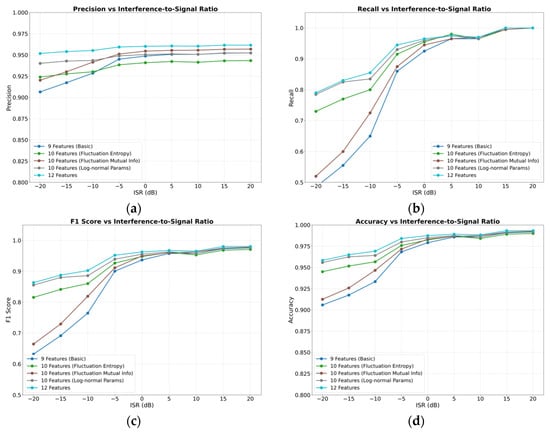
Figure 5.
Model Performance Using Different Features under Various ISR Conditions: (a) variation in precision metrics; (b) variation in recall metrics; (c) variation in F1-Score metrics; (d) variation in accuracy metrics.
A horizontal comparison of the subplots in Figure 5 reveals that as the ISR increases, the detection performance of the models gradually improves. When the ISR exceeds −5 dB, the F1-scores of all models using different features surpass 0.9. At high ISR levels, the performance of models employing different features is relatively similar. However, significant performance disparities emerge among features under low ISR conditions. To facilitate a more intuitive and precise numerical comparison of feature performance, we compiled a performance comparison table for models under low ISR conditions. In anomaly detection tasks, accuracy has inherent limitations due to the typically low proportion of anomalous samples. Conversely, recall and precision—which measure the proportion of true anomalies correctly detected and the proportion of predicted anomalies that are truly anomalous, respectively—are often conflicting metrics. In practice, the F1-score is commonly used to balance these two metrics. In this experiment, we primarily focus on the anomaly detection rate, namely recall and the F1-score, which harmonizes recall and precision. Therefore, we summarized the performance of these two metrics under low ISR conditions, as detailed in Table 1.

Table 1.
Performance of Different Features under Low ISR Conditions.
Observing Table 1, it can be seen that when using the nine baseline features for anomaly detection, both the recall and F1-score of the model are very low under low ISR conditions. At an ISR of −20 dB, the recall is only 0.4850, and the F1-score is 0.6319. When any one of the proposed features is combined with the nine baseline features, the model performance under low ISR conditions is significantly improved. Among them, the combination with the FR-MI feature yields the smallest improvement in recall with 3.5 percentage points, while the combination with the lognormal distribution fitting parameters feature achieves the largest improvement in recall as 30 percentage points. The F1-score improves by approximately 18, 3, and 22 percentage points when combining the baseline features with FE, FR-MI, and lognormal distribution fitting parameters, respectively. This demonstrates that all three proposed features effectively enhance the detection performance under low ISR conditions, with the lognormal distribution fitting parameters feature showing particularly remarkable improvement. The reason for this lies in the close relationship between this feature and the distribution characteristics of the fluctuation sequence. Anomalies caused by weak interference are difficult to identify using traditional features, especially those commonly used in the energy domain, where such anomalies may not induce noticeable changes. However, they can significantly alter the detailed distribution of the fluctuation sequence, leading to substantial changes in the lognormal distribution fitting parameters. Therefore, incorporating this feature can effectively improve the performance of radio anomaly detection.
Furthermore, we observed that while combining the baseline features with any of the proposed features improved the F1-score and recall under low ISR conditions, the F1-scores of models with different features exhibited minor fluctuations at high ISR levels, as detailed in Figure 6.
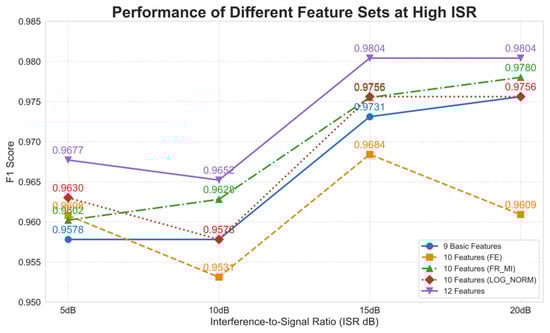
Figure 6.
Performance Comparison of Different Features at High ISR.
By synthesizing the findings from Table 1 and Figure 6, it is evident that while using the 10 features including FE significantly improves recall and F1-score under low ISR conditions, the F1-score exhibits fluctuations at high ISR levels. When the ISR exceeds 10 dB, the F1-score even falls slightly below that achieved using the original nine baseline features. In contrast, the F1-scores obtained with FR-MI or lognormal distribution fitting parameters remain comparable to those of the baseline nine features. However, when integrating all 12 features, the model not only demonstrates substantial improvements in precision, recall, F1-score, and accuracy under low ISR conditions but also maintains stable performance at high ISR levels. This can be attributed to the complementary roles of the three proposed features: they, respectively, characterize the disorder of the signal fluctuation sequence, the mutual information between adjacent fluctuations, and the overall distribution of the fluctuation sequence. Together, they capture both fine-grained variations and the holistic statistical properties of the sequence. Therefore, their combined use enhances detection performance and ensures strong robustness in complex electromagnetic environments.
5.3. Fusion Model Effectiveness Validation
To validate the performance of the proposed LOF-OCSVM anomaly detection fusion model, we conducted ablation experiments comparing it with two individual base models and two simple hybrid models based on decision-level fusion. The simple hybrid models adopted two strategies. Conservative decision strategy: a test sample is classified as anomalous only if both base models consistently identify it as anomalous; otherwise, it is classified as normal. Aggressive decision strategy: a test sample is classified as anomalous if any one of the base models identifies it as anomalous. The performance of these five models across different ISR levels was visualized, with results shown in Figure 7.
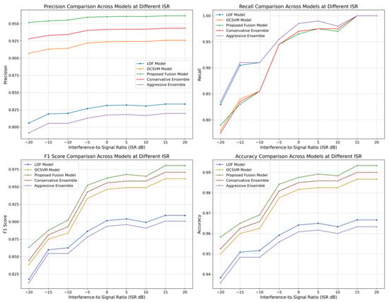
Figure 7.
Model Performance Comparison under Different ISR Conditions.
Figure 7 shows that, among the four metrics—precision, recall, F1-score, and accuracy—the proposed fusion model achieved the best performance in all except recall. Analyzing the recall and precision subplots, the LOF model and the aggressively integrated model exhibited high recall both exceeding 0.83, but their precision was significantly lower compared to other models. This reflects the inherent trade-off between recall and precision in anomaly detection tasks: high recall often indicates a tendency to capture as many anomalies as possible, which may lead to misclassifying more normal samples as anomalies thus increasing false positives and reducing precision. Conversely, high precision implies stricter criteria for identifying anomalies, potentially resulting in missed detections and lower recall. These observations align with the fundamental characteristics of anomaly detection. The F1-score effectively balances these two metrics. From the F1-score comparison, only the proposed fusion model exceeded 0.86 at a low ISR of −20 dB and maintained optimal performance across all ISR levels. In the precision subplot, the fusion model achieved a precision above 0.95 even at −20 dB ISR, indicating high accuracy in predicting anomalies at extremely low ISRs. At −10 dB ISR, the F1-score of the fusion model surpassed 0.9. Comparing the F1-scores of the conservatively and aggressively integrated models, the aggressively integrated model not only failed to balance precision and recall effectively but also underperformed in overall stability. Additionally, the accuracy comparison shows that the proposed fusion model consistently achieved the highest accuracy across all ISR levels, while the LOF model and the aggressively integrated model, despite their high recall, exhibited lower accuracy. These results demonstrate that the proposed fusion model effectively integrates the strengths of both base models, compensating for their individual limitations and achieving a balanced improvement in overall anomaly detection performance.
5.4. Comparative Experiments on Performance of Different Models
The proposed fusion model was compared with the following baseline methods: IF from traditional machine learning, artificial immune network (AINE) from bio-inspired evolutionary algorithms, Deep SVDD as a typical deep learning model, E-GAN, an innovative model proposed in reference [18]. The IF and AINE models were tested using the same set of 12 features as the proposed LOF-OCSVM model, while the two deep learning models directly took the original spectrograms as input. The reason for this approach is that deep learning models possess the inherent capability to automatically extract features. If pre-extracted features are fed into deep learning models for training and detection, it may introduce human bias that restricts the model’s ability to discover new deep feature representations, ultimately leading to suboptimal performance. To validate this hypothesis, we conducted dedicated comparative experiments on the Deep SVDD model with different input configurations before formally comparing the performance of various models. The experimental results are presented in Table 2 below:
Table 2.
F1-Scores of Deep SVDD Model under Different Input Data Configurations.
Observation of Table 2 clearly reveals that the Deep SVDD model exhibits significant performance differences under different input data configurations. The detection effectiveness when using pre-extracted feature data as input is substantially inferior to directly feeding raw spectrum data into the model for anomaly detection. This occurs because deep learning models inherently possess automated feature extraction capabilities. When processed feature data is input to such models, it may impair the deep feature extraction process, consequently affecting the model’s comprehensive understanding and mastery of the data. In contrast, traditional machine learning models and evolutionary algorithms do not involve further extraction of deep features and rely more heavily on carefully designed handcrafted features. Therefore, using preprocessed features for these models is both reasonable and necessary. Guided by this design philosophy, we conducted a comparative performance analysis of these five models, with the results presented in Figure 8.
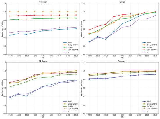
Figure 8.
Performance Comparison of Multiple Models Across Various ISR Levels.
A comprehensive analysis of the four subplots in Figure 8 reveals that the IF model from traditional machine learning and the AINE model from evolutionary algorithms underperform across all metrics, with a significant gap compared to the other three models. Among the remaining models, both the Deep SVDD and the proposed LOF-OCSVM fusion model demonstrate excellent performance, while the E-GAN model slightly lags behind. This indicates that these two deep learning models are well-suited for radio anomaly detection tasks, and the proposed fusion model, by integrating two traditional machine learning models LOF and OCSVM, achieves performance comparable to deep learning models with outstanding results. Analyzing the performance of each model across metrics, it is evident that almost all models show improved performance as the ISR increases. However, the precision of the Deep SVDD model remains constant at 1.0 regardless of ISR changes. This is due to the unique characteristics of the Deep SVDD model: it is trained exclusively on normal data without requiring a preset contamination ratio. Nevertheless, to encompass all normal training data within the hypersphere, the model may set an excessively large radius, potentially enclosing some anomalous data and leading to increased missed detections. This is reflected in the recall and F1-score subplots, where despite its strong precision, Deep SVDD’s recall is unsatisfactory, dropping below 0.8 at ISR levels of −15 dB and lower. In contrast, while the proposed fusion model does not match Deep SVDD’s precision, it still maintains a precision above 0.95 even at the lowest ISR. Moreover, it exhibits a significant advantage in recall under low ISR conditions, resulting in a higher F1-score than Deep SVDD when ISR is below −5 dB. This demonstrates that the LOF-OCSVM fusion model effectively balances precision and recall, maintaining a high F1-score even under low ISR conditions.
The above analysis reveals that both the Deep SVDD model and the proposed LOF-OCSVM fusion model demonstrate outstanding performance, with F1-scores exceeding 0.85 even at an ISR of −20 dB. Their overall performance is comparable, with the LOF-OCSVM fusion model achieving a higher F1-score under low ISR conditions, while the Deep SVDD model performs better at high ISR levels. To further compare the discriminative power of the two models in distinguishing between positive and negative samples, we plotted their ROC curves to illustrate the relationship between the true positive rate and false positive rate under different classification thresholds. The results are shown in Figure 9.
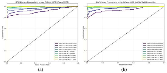
Figure 9.
ROC Curves of Different Models: (a) ROC curve of Deep SVDD model; (b) ROC curve of LOF-OCSVM model.
A comparative analysis of the two subplots in Figure 9 reveals that under weak interference conditions such as below 0 dB ISR and in most scenarios such as 15 dB ISR, the proposed LOF-OCSVM fusion model significantly outperforms the Deep SVDD model. Notably, at −20 dB ISR, the AUC value of the LOF-OCSVM fusion model reaches 0.939, substantially higher than the 0.909 achieved by Deep SVDD. However, at 5 dB and 10 dB ISR, the Deep SVDD model exhibits slightly higher AUC values than the proposed fusion model, with marginal differences of 0.001 and 0.002, respectively. At a high ISR of 20 dB, both models achieve a perfect AUC value of 1.0. Overall, the proposed LOF-OCSVM fusion model demonstrates superior performance and stronger robustness across varying ISR conditions compared to the Deep SVDD model. The Deep SVDD model exhibits greater performance fluctuations with changes in ISR, indicating lower stability than the proposed fusion model.
In addition, to evaluate the computational efficiency differences among various models, we conducted a comparative analysis of the total processing time and single-signal processing time for different models on the dataset, as detailed in Table 3 below:
Table 3.
Processing Time of Different Models on the Test Set (Unit: seconds).
From the analysis of Table 3, it can be found that AINE and IF models perform the best in terms of total time consumption. The proposed LOF-OCSVM model is the second best. The two deep learning models consume the most time, especially the E-GAN model. The reason for this is that traditional machine learning and evolutionary algorithms construct models by extracting hand-crafted features, and the complexity of these models is much lower than that of deep learning algorithms. Therefore, their computational cost is naturally much lower than that of deep models. The proposed LOF-OCSVM model, in addition to training two base models, also requires weighted integration and hierarchical decision-making during the testing phase, which incurs some computational cost. Considering the model performance analyzed earlier, the proposed LOF-OCSVM model can achieve better performance with lower computational resource consumption, thus achieving a good balance between efficiency and performance.
5.5. Multiple Models Robustness Comparison Experiment
The experiments mentioned above were all carried out on the same simulation dataset, and the performance differences in the models might be caused by the randomness of the data. Thus, in order to eliminate the randomness of a single dataset and further verify the performance stability of the models in the face of slight fluctuations in data distribution, in this section, we set 10 random seeds for the data simulation script to generate diversified datasets. Then, we record the index values of each model on the 10 datasets, calculate their mean and standard deviation, so as to evaluate the overall detection ability of the models and the fluctuation degree of model performance with data changes, and comprehensively assess the effectiveness and robustness of the models under low ISRs. We have summarized the performance of each model from −20 dB to −5 dB ISRs, as shown in Table 4.
Table 4.
Model Performance under Low ISRs.
An overall analysis of Table 4 reveals that the proposed LOF-OCSVM hybrid model excels in both performance and stability. Specifically, under the lowest ISR, its recall and F1-score both surpass 0.8. This is mainly attributed to the model’s hierarchical decision-making mechanism. By integrating scores for an initial judgment and dynamically revising low-confidence samples based on the confidence of base models, it avoids the biases of single models. For instance, while the LOF model achieves high recall, it suffers from low precision, and the OCSVM model has high precision but low recall. Moreover, the LOF-OCSVM model demonstrates robustness with a standard deviation between 0.00 and 0.03. This is because the weighted integration strategy combines LOF’s local density sensitivity with OCSVM’s global boundary learning. The complementary nature of these two models reduces the impact of data fluctuations on detection results. When local data distribution changes, OCSVM’s global decision-making provides stability. When global data distribution shifts, LOF’s local density analysis can compensate for deviations. The base models and simple fusion models also meet robustness standards with a deviation between 0.01 and 0.03. However, they have performance shortcomings. The LOF model has a high average recall but a low average F1-score, indicating it focuses too much on local anomalies and misclassifies normal samples as anomalies, leading to low precision and a compromised F1-score. The OCSVM model has a high F1-score but lower average recall than LOF. This is because OCSVM relies on global boundaries in high-dimensional spaces and struggles to detect local weak anomalies. The aggressive and conservative fusion models consistently face a precision-recall trade-off and underperform compared to the LOF-OCSVM model. This indicates that simple decision-level fusion cannot match the advantages of weighted integration and hierarchical correction. The AINE model has comparable robustness but significantly lags in performance. This is because, under low ISRs, the subtle differences between weak interference and normal signals blur the self-sample boundaries of the AINE model, reducing its anomaly identification accuracy. Additionally, the high computational complexity of AINE’s immune network iteration process limits its performance potential in low ISR scenarios. In contrast, the IF, Deep SVDD, and E-GAN models show a marked increase in standard deviation. Their performance varies greatly across different datasets, indicating poor robustness and significant fluctuations in performance metrics. The IF model performs the worst with low average metrics and high variance. This may be due to its sensitivity to data distribution randomness. When local data density varies with different random seeds, the structure of isolated trees changes significantly, causing detection results to fluctuate. Deep SVDD and E-GAN also perform poorly in terms of average metrics and standard deviation. Deep SVDD may inadvertently enlarge the hypersphere containing normal samples, including some anomalies. E-GAN suffers from unstable training, mode collapse, and high sensitivity to data distribution changes. These issues exacerbate performance fluctuations across datasets.
To better illustrate how different models perform across varying ISRs, we plotted the average F1-scores and recall rates of each model in Figure 10.
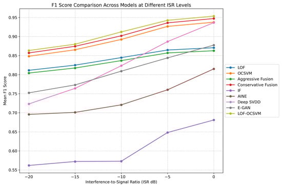
Figure 10.
F1-scores of Various Models across Different ISRs.
As shown in Figure 10, all models’ performance improves with increasing ISR, in line with previous findings. This indicates that despite potential performance variations due to randomness in a single dataset, it can still reflect the overall trend of model performance across different ISRs. In terms of the rate of improvement, the Deep SVDD model has the steepest slope, followed by the E-GAN model. This suggests that these two models are more sensitive to changes in ISR. Their performance is relatively poor at low ISRs but shows a tendency to surpass other models at higher ISRs. However, overall, their performance is heavily influenced by ISR, making them less capable of adapting to complex electromagnetic environments with low ISRs. Combined with standard deviation analysis, it is evident that the performance of these models fluctuates significantly with changes in data distribution. Consequently, they require continuous parameter tuning to adapt to different datasets, which limits their generalization and universality. On the other hand, the proposed LOF-OCSVM hybrid model exhibits a steady upward trend and consistently outperforms all other models. It demonstrates a strong ability to adapt to subtle changes in data distribution and complex electromagnetic conditions across different ISRs.
In addition, we further verified the effectiveness of our method by testing the model’s performance on the public dataset RML2016.10a [29]. During the experiment, we chose the 8PSK modulated signals for testing and drew heat maps of F1 score for LOF, OCSVM, and the integrated LOF-OCSVM model, which are shown in Figure 11.
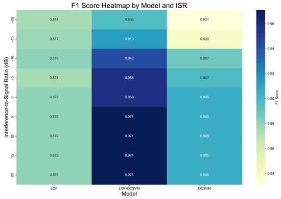
Figure 11.
Heatmap of Model F1-Scores on the RML2016.10a Dataset.
As shown in the F1-score heatmap of the RML2016.10a dataset, the LOF-OCSVM model still has remarkable performance improvement compared to single base models. The LOF model’s scores are stable but with light colors, indicating limited superiority. The OCSVM model is most affected by ISR, with poor performance and stability under low ISRs. The LOF-OCSVM model shows dark-colored areas across the ISR range, meaning high and evenly distributed F1-scores. At −20 dB ISR, its F1-score is approximately 2% and 8% higher than the LOF and OCSVM models, verifying the effectiveness and generalization ability of the method in near–real scenarios.
6. Conclusions
This paper addresses the performance bottleneck of radio anomaly detection in low ISR conditions. We propose three features based on fluctuation sequences: fluctuation entropy, fluctuation mutual information, and lognormal distribution fitting parameters of fluctuation sequences. And we design a LOF-OCSVM hybrid detection algorithm. Through weighted score integration and hierarchical decision-making, it dynamically corrects low-confidence samples and balances the trade-off between recall and precision. Simulation experiments show that our method excels in detecting radio anomalies in extremely low ISRs (−20 dB). It achieves a recall rate and F1-score of over 0.8,with a minimum AUC of 0.939. The model also demonstrates strong robustness across different ISRs. Our future work includes exploring cross-modal fusion of fluctuation and deep features to enhance the model’s ability to detect weak anomalies. We also aim to optimize the weighting strategy in our fusion model by incorporating adaptive learning to boost robustness further. Lastly, we will work on reducing the model’s computational complexity to better suit the resource requirements of real-time spectrum monitoring.
Author Contributions
Conceptualization, Y.Z. and X.Z.; methodology, Y.Z. and L.C.; software, Y.Z.; validation, Y.Z., Y.M., and M.Y.; formal analysis, Y.Z. and X.Z.; investigation, Y.Z. and M.Y.; resources, Y.Z. and L.C.; data curation, Y.Z. and Y.M.; writing—original draft preparation, Y.Z.; writing—review and editing, Y.M. and M.Y.; visualization, Y.Z.; supervision, X.Z.; project administration, L.C.; funding acquisition, X.Z. All authors have read and agreed to the published version of the manuscript.
Funding
This research was funded by the National Natural Science Foundation of China, grant number 62276273, “Research on Key Technologies of Data Security in Multi-Cloud Storage Based on Zero-Trust Architecture”. The APC was funded by the same grant.
Data Availability Statement
The raw data supporting the conclusions of this article will be made available by the authors on request.
Conflicts of Interest
The authors declare no conflicts of interest. The funders had no role in the design of the study; in the collection, analyses, or interpretation of data; in the writing of the manuscript; or in the decision to publish the results.
Abbreviations
The following abbreviations are used in this manuscript:
| ISR | interference-to-signal ratio |
| LOF | local outlier factor |
| OCSVM | one-class support vector machine |
| FE | fluctuation entropy |
| FR-MI | fluctuation mutual information |
| Deep SVDD | deep support vector data description |
| CME | consecutive mean excision |
| FCME | forward consecutive mean excision |
| SNR | signal-to-noise ratio |
| SVM | support vector machine |
| DT | decision tree |
| IF | isolation forest |
| LSTM | long short-term memory |
| CNN | convolutional neural network |
| GAN | generative adversarial network |
| STFT | short-time fourier transform |
| OFDM | orthogonal frequency division multiplexing |
| QPSK | quadrature phase shift keying |
| CDF | cumulative distribution function |
| AINE | artificial immune network |
| ROC | receiver operating characteristic |
| AUC | area under curve |
References
- Urkowitz, H. Energy detection of unknown deterministic signals. Proc. IEEE 1967, 55, 523–531. [Google Scholar] [CrossRef]
- Henttu, P.; Aromaa, S. Consecutive mean excision algorithm. In Proceedings of the IEEE Seventh International Symposium on Spread Spectrum Techniques and Applications, Prague, Czech Republic, 2–5 September 2002; Volume 2, pp. 450–454. [Google Scholar] [CrossRef]
- Saamisaari, H.; Henttu, P. Impulse detection and rejection methods for radio systems. In Proceedings of the IEEE Military Communications Conference, Boston, MA, USA; 2003; Volume 2, pp. 1126–1131. [Google Scholar] [CrossRef]
- Sun, Q. Research and Implementation of Radio Signal Anomaly Detection Algorithm. Master’s Thesis, Beijing University of Posts and Telecommunications, Beijing, China, 2019. [Google Scholar]
- Wu, X. Research on Spectrum Anomaly Detection Technology for Management of Radio. Master’s Thesis, University of Electronic Science and Technology of China, Chengdu, China, 2021. [Google Scholar]
- Masari, A.O.; Ahmad, A.A.; Lawan, S.; Muhammad, B. Comparison Analysis of Static and Dynamic Thresholds for Conventional Cognitive Radio Spectrum Sensing Methods. In Proceedings of the 2024 IEEE 5th International Conference on Electro-Computing Technologies for Humanity (NIGERCON), Ado Ekiti, Nigeria, 26–28 November 2024; pp. 1–4. [Google Scholar] [CrossRef]
- Liang, X. Research on Interference Detection and Identification Technology of Beidou Civil Signal. Master’s Thesis, Civil Aviation University of China, Tianjin, China, 2020. [Google Scholar]
- Zhang, S. Research on Interference Detection and Direction Finding Technology of Beidou Civil Signal. Master’s Thesis, Civil Aviation University of China, Tianjin, China, 2021. [Google Scholar]
- Jiu, Y.; Liu, J.; Meng, J.; Yang, S.; Li, R.; Duan, H. Identification Method of Blocking Interference for Railway Wireless Communication Based on ACMD and Spectrum Sensing. J. China Railw. Soc. 2025, 47, 82–90. [Google Scholar] [CrossRef]
- Xiong, Y.; Wang, J. Application of Improved Ant Colony Algorithm in Automatic Recognition of Abnormal Signals in Wireless Communication Networks. In Proceedings of the 2023 International Conference on Data Science and Network Security (ICDSNS), Tiptur, India, 28–29 July 2023; pp. 1–5. [Google Scholar] [CrossRef]
- Ma, J.; Zhong, Z.F.; Zou, X.; Shi, Y.C. Anomalistic Electromagnetism Signal Detection Model Based on Immune Network. Appl. Res. Comput. 2011, 28, 2140–2143. [Google Scholar]
- Ma, J.; Zhong, Z.; Huang, G. An Adaptive Variable Weighting Immune Network Algorithm for Electromagnetism Signal Monitoring. J. Beijing Univ. Posts Telecommun. 2012, 35, 59–63. [Google Scholar]
- Ma, J.; Shi, Y.; Zhong, Z. An Anomalistic Electromagnetism Signal Monitoring Based on Artificial Immune System. Fire Control Command Control 2012, 37, 89–92+95. [Google Scholar]
- Feng, B. Recognition Research of Abnormal Radio Signal Based on Support Vector Machine. Master’s Thesis, Xihua University, Chengdu, China, 2014. [Google Scholar] [CrossRef]
- Yu, F.; Yue, W.; Chen, Z. Single User Spectrum Sensing Algorithm Based on Kernel Space Optimization SVM. Comput. Technol. Dev. 2023, 33, 180–186. [Google Scholar] [CrossRef]
- Pang, J.; Pu, X.; Li, C. A Hybrid Algorithm Incorporating Vector Quantization and One-Class Support Vector Machine for Industrial Anomaly Detection. IEEE Trans. Ind. Inform. 2022, 18, 8786–8796. [Google Scholar] [CrossRef]
- Qi, Y. Electromagnetic Frequency Spectrum Monitoring System Design and Implementation. Master’s Thesis, University of Electronic Science and Technology of China, Chengdu, China, 2019. [Google Scholar]
- Feng, X. Research on Eletromagnetic Spectrum Intrusive Signal Detection Technology. Master’s Thesis, Beijing University of Posts and Telecommunications, Beijing, China, 2019. [Google Scholar]
- Wang, Y. Research on Multi-interference Detection and Recognition Method Based on Feature Extraction. Master’s Thesis, University of Electronic Science and Technology of China, Chengdu, China, 2022. [Google Scholar]
- Yengi, Y.; Kavak, A.; Arslan, H. Physical Layer Detection of Malicious Relays in LTE-A Network Using Unsupervised Learning. IEEE Access 2020, 8, 154713–154726. [Google Scholar] [CrossRef]
- Hong, S.; Kim, K.; Lee, S.-H. A Hybrid Jamming Detection Algorithm for Wireless Communications: Simultaneous Classification of Known Attacks and Detection of Unknown Attacks. IEEE Commun. Lett. 2023, 27, 1769–1773. [Google Scholar] [CrossRef]
- Ford, G.; Foster, B.J.; Braun, S.A.; Kam, M. Unknown Signal Detection in Switching Linear Dynamical System Noise. IEEE Trans. Signal Process. 2023, 71, 2220–2234. [Google Scholar] [CrossRef]
- Rajendran, S.; Meert, W.; Lenders, V.; Pollin, S. Unsupervised Wireless Spectrum Anomaly Detection with Interpretable Features. IEEE Trans. Cogn. Commun. Netw. 2019, 5, 637–647. [Google Scholar] [CrossRef]
- Kulin, M.; Kazaz, T.; Moerman, I.; De Poorter, E. End-to-End Learning from Spectrum Data: A Deep Learning Approach for Wireless Signal Identification in Spectrum Monitoring Applications. IEEE Access 2018, 6, 18484–18501. [Google Scholar] [CrossRef]
- Zhou, X.; Xiong, J.; Zhang, X.; Liu, X.; Wei, J. A Radio Anomaly Detection Algorithm Based on Modified Generative Adversarial Network. IEEE Wirel. Commun. Lett. 2021, 10, 1552–1556. [Google Scholar] [CrossRef]
- Sun, D.; Lu, S.; Wang, W. CAAE: A Novel Wireless Spectrum Anomaly Detection Method with Multiple Scoring Criterion. In Proceedings of the 2021 28th International Conference on Telecommunications (ICT), London, UK, 1–3 June 2021; pp. 1–5. [Google Scholar] [CrossRef]
- Zeng, J.; Liu, X.; Li, Z. Radio Anomaly Detection Based on Improved Denoising Diffusion Probabilistic Models. IEEE Commun. Lett. 2023, 27, 1979–1983. [Google Scholar] [CrossRef]
- Li, Y.; Li, X.; Lv, S.; Chen, Y.; Zhang, W.; Ding, Y. Unsupervised Anomaly Detection for IoT Time Series Signals with GANs. In Proceedings of the 2024 IEEE International Conference on Signal, Information and Data Processing (ICSIDP), Zhuhai, China, 22–24 November 2024; pp. 1–6. [Google Scholar] [CrossRef]
- O’Shea, T.J.; Corgan, J.; Clancy, T.C. Convolutional radio modulation recognition networks. In Proceedings of the International Conference on Engineering Applications of Neural Networks, Aberdeen, UK, 2–5 September 2016; Springer International Publishing: Cham, Switerland, 2016; pp. 213–226. [Google Scholar]


Disclaimer/Publisher’s Note: The statements, opinions and data contained in all publications are solely those of the individual author(s) and contributor(s) and not of MDPI and/or the editor(s). MDPI and/or the editor(s) disclaim responsibility for any injury to people or property resulting from any ideas, methods, instructions or products referred to in the content. |
© 2025 by the authors. Licensee MDPI, Basel, Switzerland. This article is an open access article distributed under the terms and conditions of the Creative Commons Attribution (CC BY) license (https://creativecommons.org/licenses/by/4.0/).