Research on Preventive Maintenance Technology for Highway Cracks Based on Digital Image Processing

Abstract

Cracks are the initial manifestation of various diseases on highways. Preventive maintenance of cracks can delay the degree of pavement damage and effectively extend the service life of highways. However, existing crack detection methods have poor performance in identifying small cracks and are unable to calculate crack width, leading to unsatisfactory preventive maintenance results. This article proposes an integrated method for crack detection, segmentation, and width calculation based on digital image processing technology. Firstly, based on convolutional neural network, a optimized crack detection network called CFSSE is proposed by fusing the fast spatial pyramid pooling structure with the squeeze-and-excitation attention mechanism, with an average detection accuracy of 97.10%, average recall rate of 98.00%, and average detection precision at 0.5 threshold of 98.90%; it outperforms the YOLOv5-mobileone network and YOLOv5-s network. Secondly, based on the U-Net network, an optimized crack segmentation network called CBU_Net is proposed by using the CNN-block structure in the encoder module and a bicubic interpolation algorithm in the decoder module, with an average segmentation accuracy of 99.10%, average intersection over union of 88.62%, and average pixel accuracy of 93.56%; it outperforms the U_Net network, DeepLab v3+ network, and optimized DeepLab v3 network. Finally, a laser spot center positioning method based on information entropy combination is proposed to provide an accurate benchmark for crack width calculation based on parallel lasers, with an average error in crack width calculation of less than 2.56%.

1. Introduction

Cracks are one of the most common, easily occurring, and early developing among various types of pavement diseases. They accompany the entire service life of the highway and worsen with the increase in road age. The harm of highway cracks does not only affect the aesthetic appearance and driving comfort of the road, but also causes structural damage to the highway if cracks are not sealed and repaired in a timely manner, allowing rainwater and other debris to enter the surface structure and subgrade along the cracks, leading to a decrease in the road’s bearing capacity. This article studies the integrated technology of crack detection, segmentation, and width calculation, which can accurately detect and quantify cracks, enabling highway maintenance departments to carry out preventive repair work on cracks in the early stages, preventing further expansion of cracks, extending the service life of highways, and promoting the sustainable development of highways.

In the field of crack detection, some scholars use single-stage object detection networks, such as the You Only Look Once (YOLO) network [1,2,3,4]. This type of network has high efficiency and a simple structure, but, due to directly predicting target position and category, its detection accuracy is relatively low and easily affected by background interference. Some scholars use two-stage object detection networks, such as convolutional neural network (CNN) [5,6,7,8,9], which filters background noise effectively and improves detection accuracy through candidate region generation, precise position regression, and classification in two stages, making it especially suitable for cases with partial occlusion, complex shapes, or varying sizes. However, these networks have higher complexity and relatively slower processing speeds. In recent years, the emergence of network models such as RetinaNet and Transformer has increased the depth and width of network structures, resulting in more accurate and complete extraction of image features. Networks based on these models, including classification and object detection networks, have been effectively applied to crack detection tasks in highways. These advanced network models provide a more accurate and efficient solution for crack detection, helping to improve the efficiency and quality of highway maintenance [10,11,12].

In crack segmentation, some scholars use the U-Net segmentation network [13,14,15]. The U-Net network evolved from the fully convolutional network (FCN) [16] and innovatively introduced the use of skip connections to connect shallow features with deep features, enabling the full utilization of shallow features for higher segmentation accuracy. Some scholars utilize the SegNet segmentation network [17,18,19], which also evolved from the FCN network [20]. The down-sampling process of the SegNet network uses the Visual Geometry Group (VGG) structure to extract image features. Additionally, some scholars employ the Deeplab segmentation network [21,22,23]. With the continuous development of the Deeplab series, its performance has been consistently improving. For example, Deeplab v3+ builds upon Deeplab v3 by adding a semantic branch, effectively integrating boundary information and enhancing edge segmentation results.

In crack width calculation, some scholars utilize image processing-based methods for crack width calculation [24,25,26]. This method typically includes steps such as image preprocessing, feature extraction, and crack width calculation. In practical applications, to convert pixel width to actual crack width, pixel calibration is required. This is often achieved by placing a known physical length reference object in the image, such as parallel laser beams. By measuring the pixel length of the reference object in the image, the actual length represented by each pixel can be calculated, thereby obtaining the actual width of the crack.

In summary, standalone crack detection has limited practical significance as it cannot extract crack information from images to determine width and other details. Therefore, it is necessary to integrate it with image segmentation algorithms such as U-Net. After extracting cracks from images through segmentation, without a reference point, only the pixel location of the crack in the image can be obtained, making it impossible to measure the actual width of the crack. Existing crack width measurement methods based on parallel laser beams assume the laser spot to be an ideal circle. However, in practical measurements, the spot may become irregular in shape due to beam divergence and surface irregularities, leading to significant errors in crack width measurements using existing parallel laser-based methods in real-world applications.

The specific research structure and innovations of this article are as follows:

• In Section 2, a novel highway crack detection network is proposed, based on convolutional neural network, integrating the fast spatial pyramid pooling structure and the squeeze–excitation attention mechanism.
• In Section 3, a novel highway crack segmentation network is introduced, based on the U-Net network, with the down sampling module using the CNN-block structure and the up-sampling module employing the bicubic interpolation algorithm.
• In Section 4, a novel highway crack width calculation method is presented, utilizing the ellipse fitting method and grayscale centroid method, and employing an information entropy model to locate the center of the laser spot.
• In Section 5, a series of experiments are conducted to validate the effectiveness of the method proposed in this article, and the results are analyzed from both a numerical and visual perspective.

2. Establish a Highway Crack Detection Network

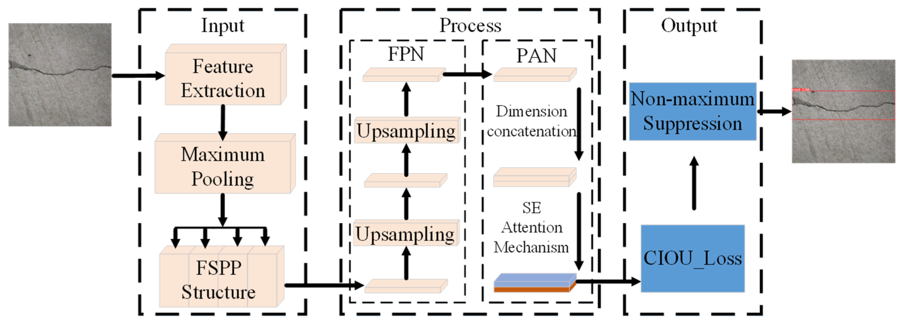
Currently existing crack detection methods have problems such as incomplete crack detection and low detection accuracy. In this article, from the perspective of improving the crack detection capability, we propose a crack detection network based on convolutional neural network, and fusion of fast spatial pyramid pooling structure (FSPP) and squeeze–excitation attention mechanism (SE), referred to as the CFSSE network, whose structure is shown in Figure 1.

2.1. Fast Space Pyramid Pooling Structure

The convolutional neural network with fully connected layers requires a uniform format of image input, while in the actual crack image dataset, the size of the crack image is not consistent, and the aspect ratio of each crack is also different. If we take measures such as cutting and stretching to rigidly standardize the ratio and size of the image, it will cause distortion of the original image and make it easy to lose the key information of cracks, which will have a negative impact on the training of the network.

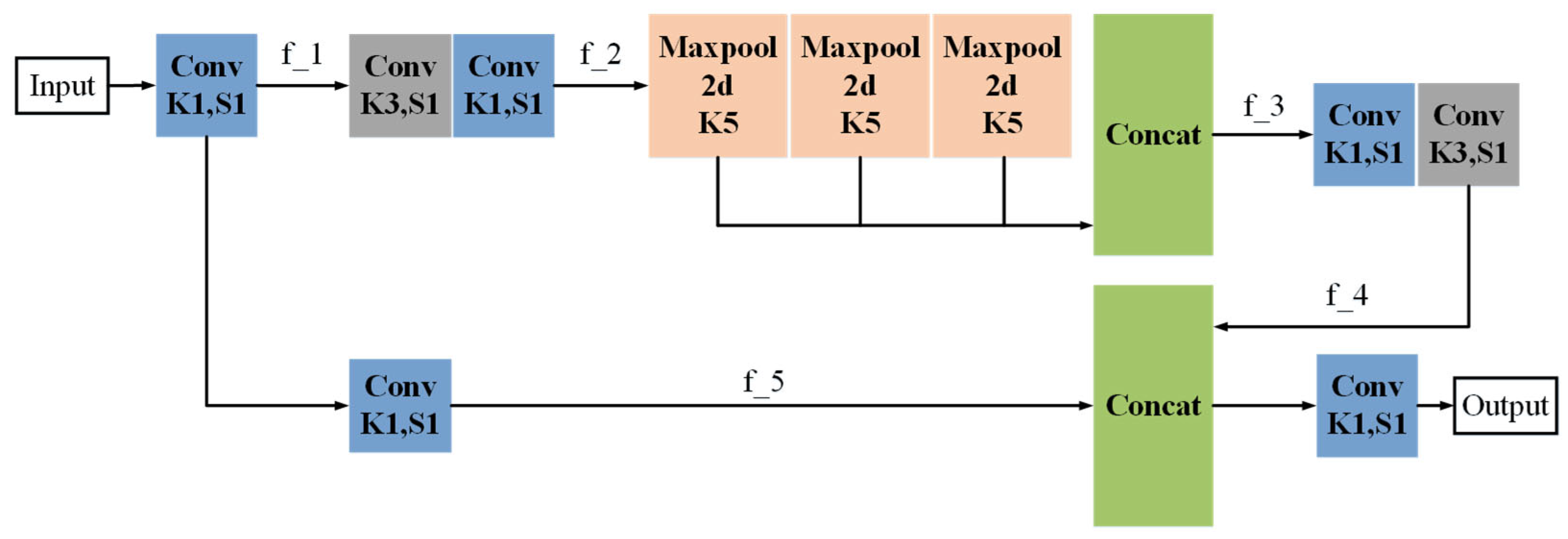
To address this issue, this article introduces a fast spatial pyramid pooling structure, as shown in Figure 2. The input is first passed through a convolutional kernel of size 1 × 1 to obtain the feature map f_1 through a compression channel. Subsequently, the feature map f_2 is obtained through two convolutional channels with kernel sizes of 3 × 3 and 1 × 1. The feature map f_3 is obtained through a series of successive maximum pooling structures and concatenation. Then, the feature map f_4 is obtained by passing f_3 through two convolutional channels with kernel sizes of 3 × 3 and 1 × 1. After passing the input through a 1 × 1 convolutional channel to obtain the feature map f_5, concatenation is performed between f_4 and f_5. Finally, the output is obtained through another 1 × 1 convolutional channel, enabling the input image data to be of arbitrary size.

2.2. Squeeze–Excitation Attention Mechanism

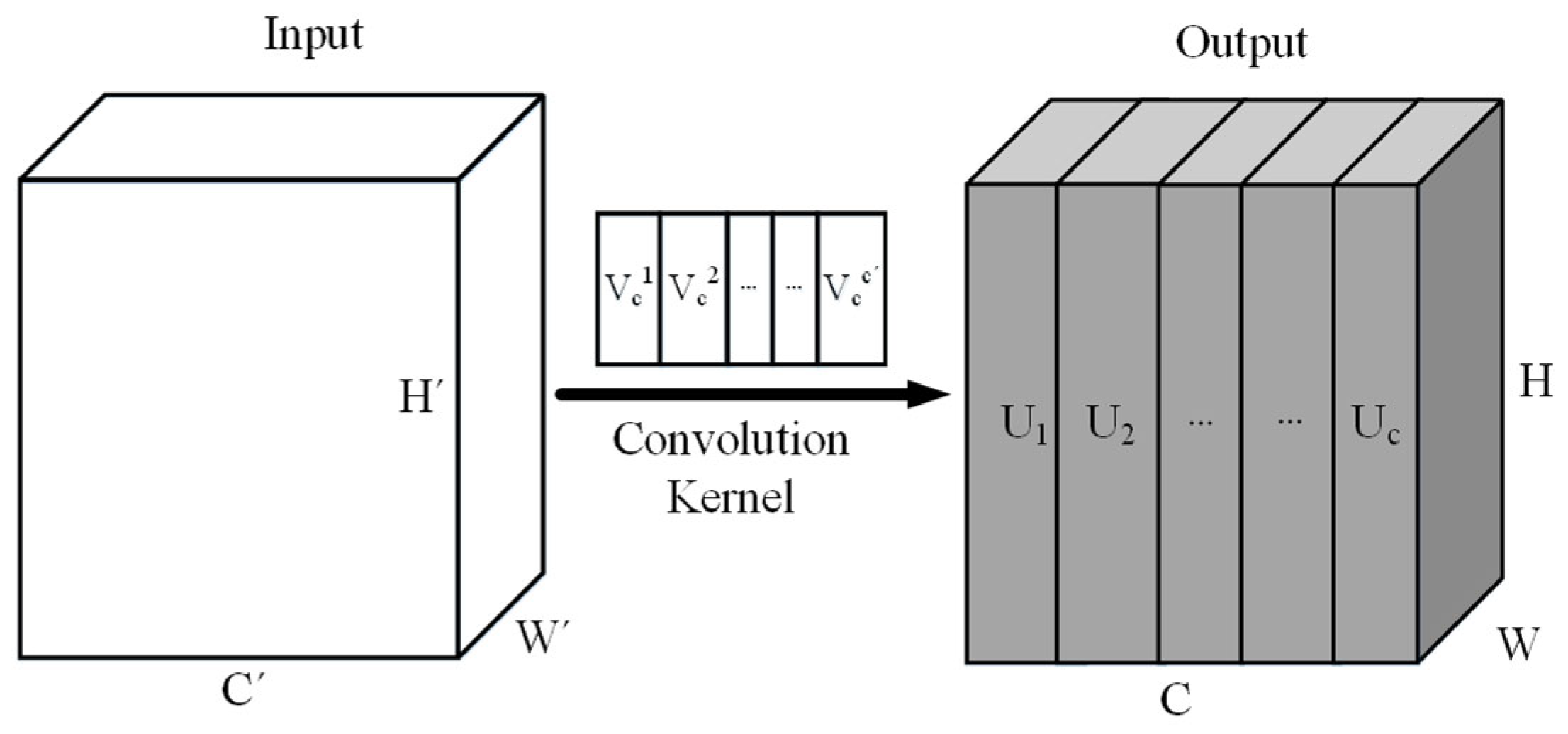
The convolution operation is shown in Figure 3, where the input $X\in R^{W^{\prime }\times H^{\prime }\times C^{\prime }}$, the output $U\in R^{H\times W\times C}$, and the convolution kernel applied to the input X is $\left[V_c^1,V_c^2,\dots ,V_c^{c^{\prime }}\right]$, the output $U_c$ is calculated as $U_c={\sum }_{s=1}^{c^{\prime }}{V}_c^s\ast X^s$. Here $V_c^s$ is a 2D spatial kernel that acts only on the corresponding individual channels, and the captured spatial features have dependencies only with the individual channels. As all the feature channels are treated equally, all the channel $\left[V_c^1,V_c^2,\dots ,V_c^{c^{\prime }}\right]$ weight values are the same. It is often difficult for the network to focus its attention on important features that are useful for the crack detection task, which results in some important features in the feature channels being ignored. In order to address this shortcoming, this article proposes the method of fusing the squeezing–excitation attention mechanism.

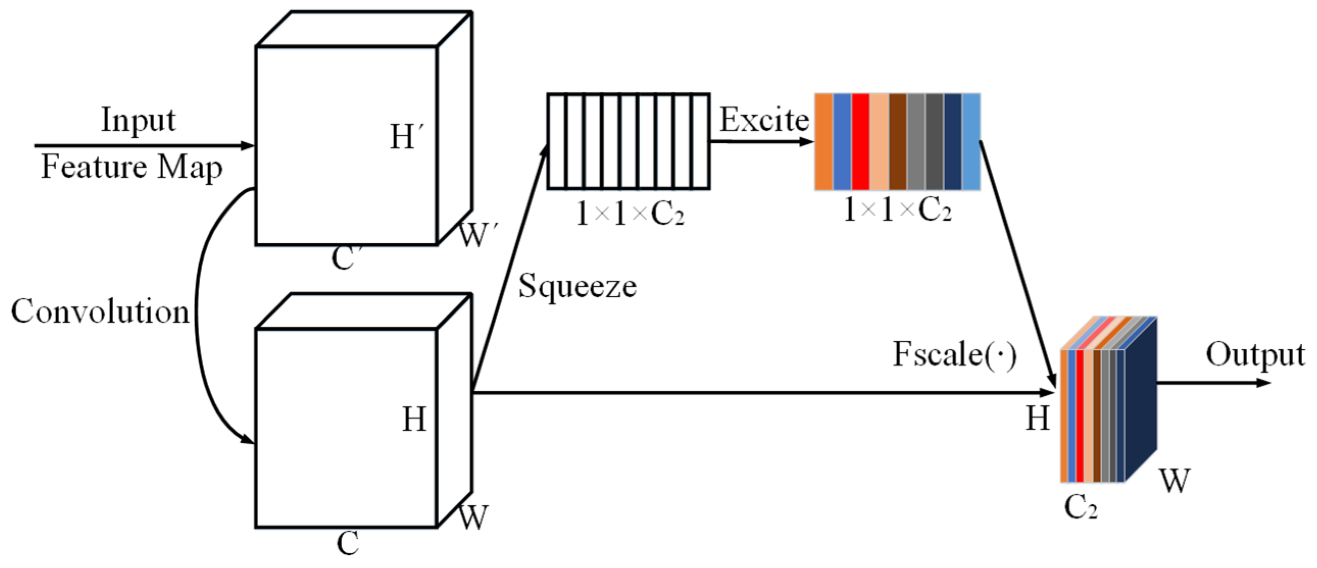
The squeeze–excitation attention mechanism module initially compresses the crack feature maps extracted by the convolutional neural network to obtain the weight of each channel, which reflects the importance of each channel for feature extraction, and then initiates the excitation procedure for the overall feature mapping network, multiplying each channel with its corresponding weight proportionally. In this way, the training results of the feature mapping channels that are useful for crack detection are enhanced, while the influence of the feature mapping channels that are not very helpful for the task is constrained, and the structure is shown in Figure 4.

The squeezing operation is performed by means of global average pooling, which aims to enlarge the scope of the perceptual domain and centrally encode all features in a given dimension of space into a single global feature, formalized as shown in Formula (1).

$$\begin{array}{c}z=f_{sq}\left(x\right)={\displaystyle \frac{1}{H\times W}}{\displaystyle \sum _{i=1}^H}{\displaystyle \sum _{j=1}^W}{x}_{i,j}\end{array}$$

(1)

where $z$ denotes the global features, $f_{sq}$ denotes the squeezing operation, $x$ denotes the input feature map, $H$ is the height of the feature map, $W$ is the width of the feature map, and $x_{i,j}$ denotes the feature vector of pixels in the i row and j column. By average pooling, the feature maps are merged and compressed from H × W × channel to 1 × 1 × channel. The latter in a single channel is obtained in the original feature map H × W receptive fields within the channels, obtaining the global description of the features.

The incentive operation reveals the inter-correlation of different channels and helps to select the information-rich channels while restricting the less informative ones, which is formalized as shown in Formula (2).

$$s=f_{ex}\left(z,W\right)=\sigma \left(W_{2\delta }\left(W_{1z}\right)\right)$$

(2)

where $s$ denotes the incentive score vector, $f_{ex}$ denotes the incentive operation, $W_1\in R^{{\displaystyle \frac{C}{r}}\times C}$ denotes the ${\displaystyle \frac{C}{r}}$ row and C column of the weight matrix, $W_2\in R^{C\times {\displaystyle \frac{C}{r}}}$ denotes the weight matrix of the C row and ${\displaystyle \frac{C}{r}}$ column, r denotes the scaling ratio, and $\sigma$ is the activation function $f\left(x\right)={\displaystyle \frac{1}{1+e^{-x}}}$. This function has the continuous derivative property, which ensures the smoothness of the gradient value and avoids the drastic change of the gradient in the model learning stage, prevents the drastic fluctuation of the output result.

3. Establish a Highway Crack Segmentation Network

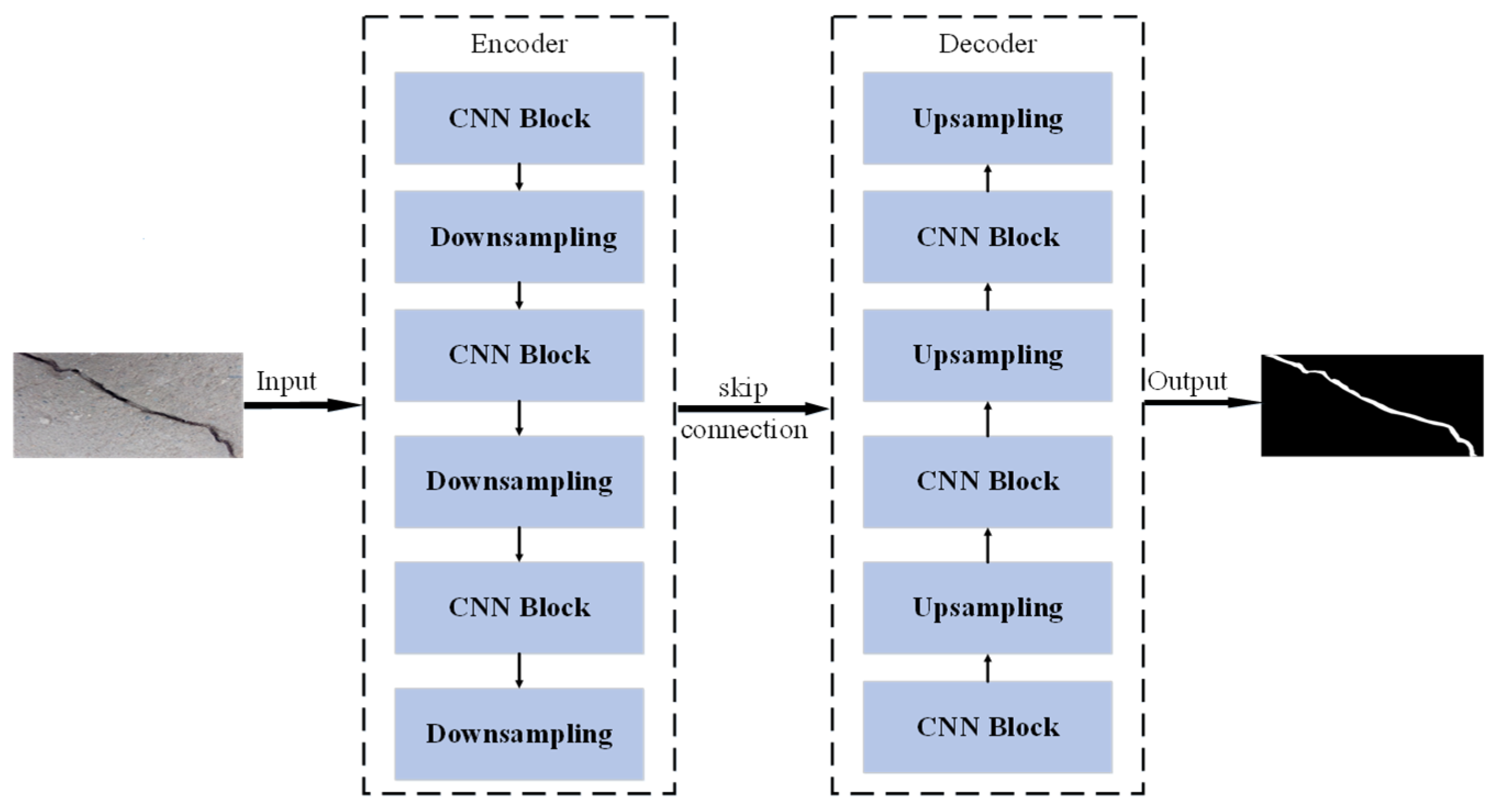
At present, the U-Net network applied to crack image segmentation has problems such as inaccurate edge segmentation and blurred boundaries; in this study, we optimize the encoder and decoder modules of U-Net, and construct a crack segmentation network (CBU-Net, as shown in Figure 5) by integrating existing modules including CNN-block, FSPP, SE, and bicubic interpolation, along with an entropy fusion mechanism. As the original manuscript lacks explanations for the optimality of this specific module combination and its generalization beyond crack detection, we supplement a systematic ablation study to quantify the individual contributions of each core component (SE, FSPP, bicubic interpolation, and entropy fusion) by comparing baseline models with sequential removal/replacement of components, and further discuss the network’s potential adaptability to other surface defect detection tasks.

3.1. Encoder Module Optimization

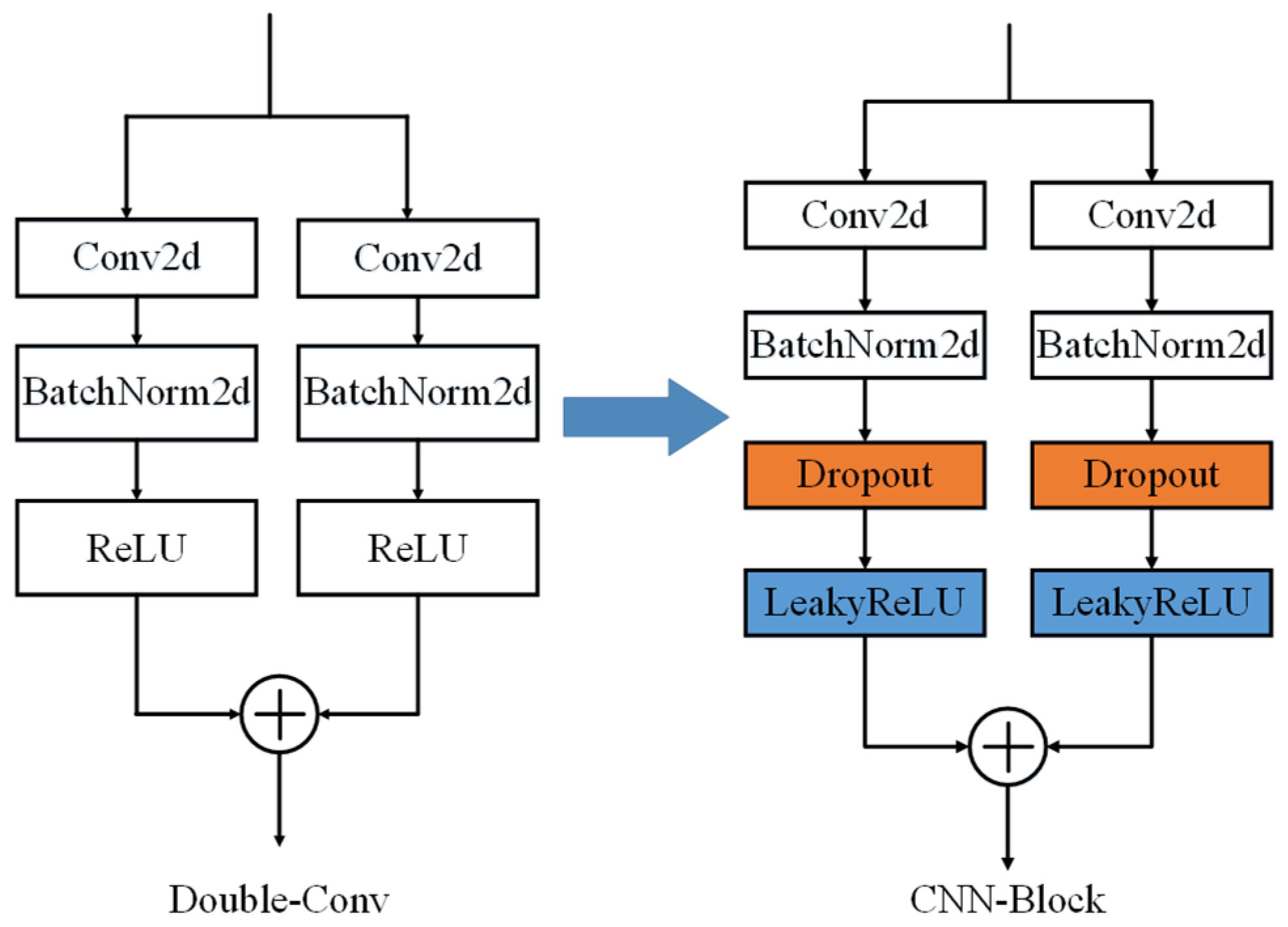
The U-Net network encoder module is mainly responsible for the downsampling operation. Due to the large and complex crack segmentation data, in order to avoid overfitting during the training process of the U-Net network and to enhance the generalization ability of the U-Net network, as shown in Figure 6, the residual inverted structure of the CNN-block structure is used instead of the original Double-Conv structure.

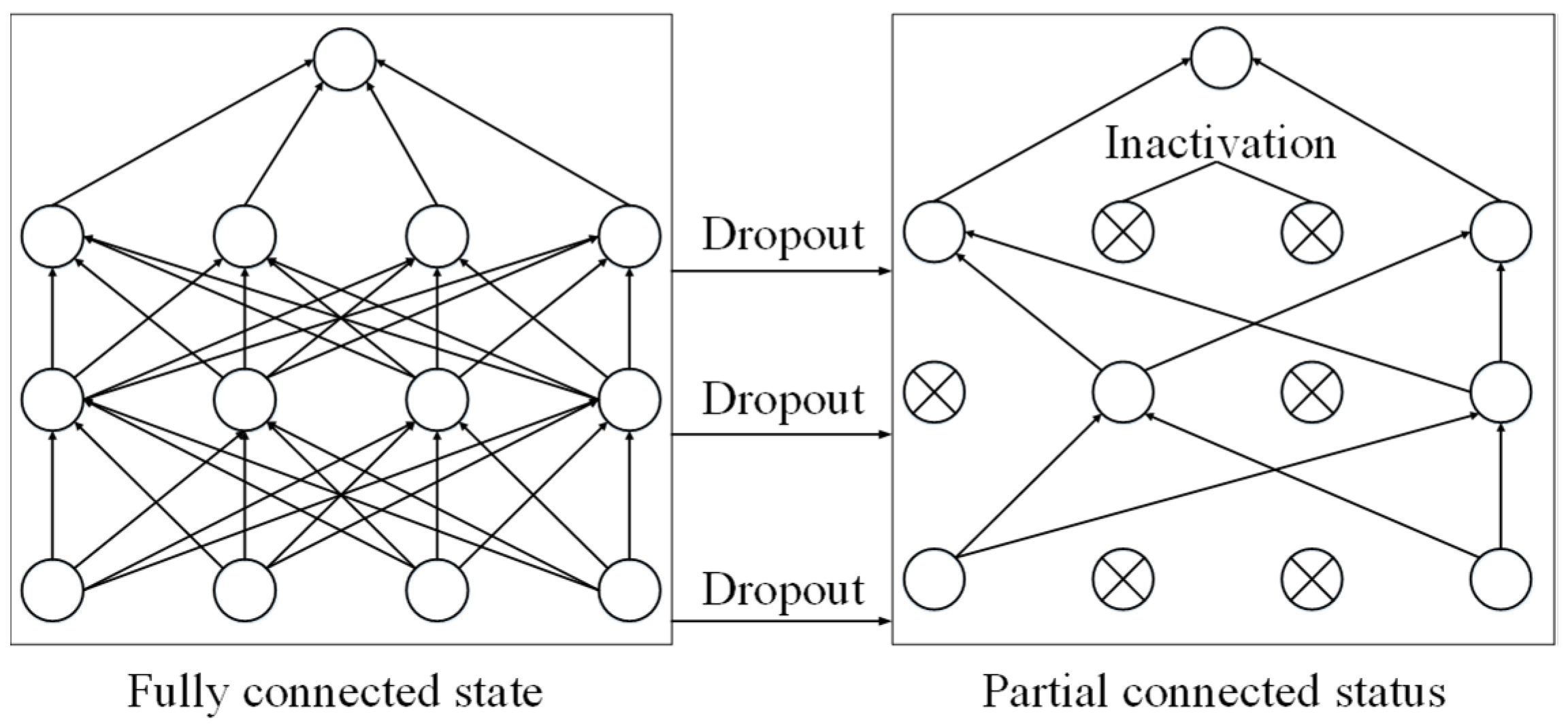
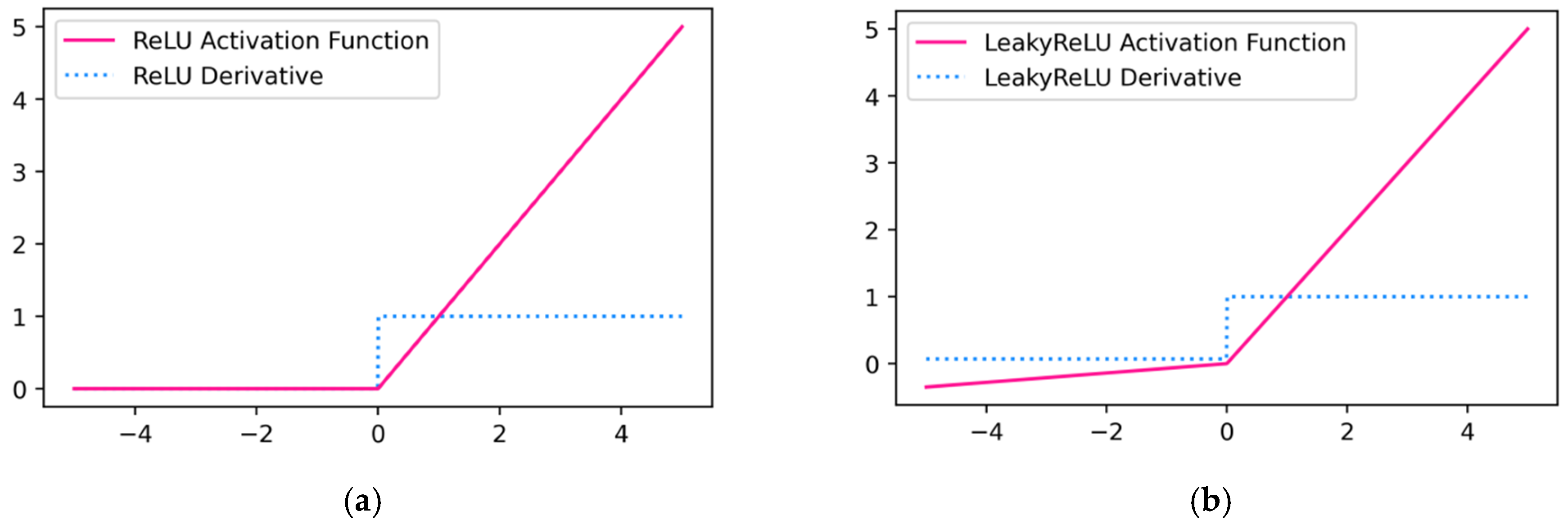
Firstly, the replaced CNN-block structure adds the Dropout regularization method in the convolutional layer, as shown in Figure 7, and the Dropout operation deactivates the neurons with a certain probability during the training process, which reduces the overdependence of the neurons on a certain feature, and is able to prevent the occurrence of neuronal co-adaptation. Secondly, the original Double-Conv structure uses the ReLU activation function, as shown in Figure 8a, which has a slope of 0 when the input is negative, thus making the corresponding neurons continuously inactive and unable to adjust their internal parameters. To solve this problem, this article uses the activation function with leakage-corrected linear unit, as shown in Figure 8b, which is activated by applying a small linear section of the input to the negative input. A portion is applied to the negative input, which in turn enhances the characterization of the activation function to extend into the negative range.

3.2. Decoder Module Optimization

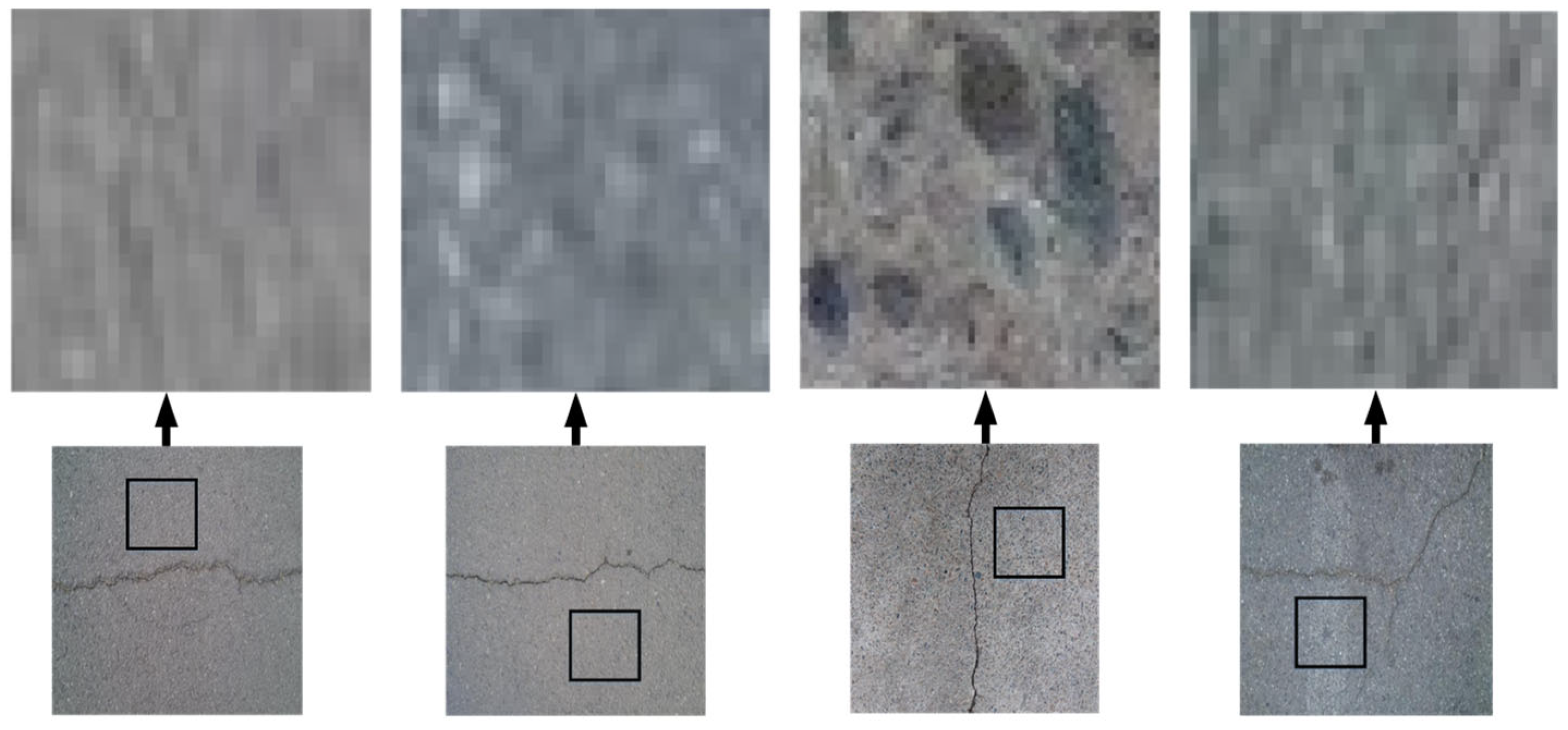
When the crack image undergoes downsampling operation, some detailed information will be lost, which can be recovered by upsampling operation through the decoder module. In the upsampling process, the non-equal coverage of the transpose-convolution operation causes the crack image to have a square pixel distribution similar to a chess board, referred to as the checkerboard effect, as shown in Figure 9. The phenomenon of uneven overlapping of feature mappings during the transpose-convolution process can be avoided by interpolating the crack image and thus changing the size of the feature image, but the bi-linear interpolation algorithm used by U_Net network has limited effect in dealing with it, as shown in Figure 9, and there is still the problem of pixel blocks when zooming in the image.

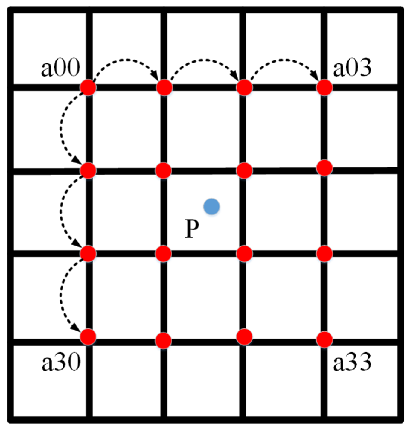
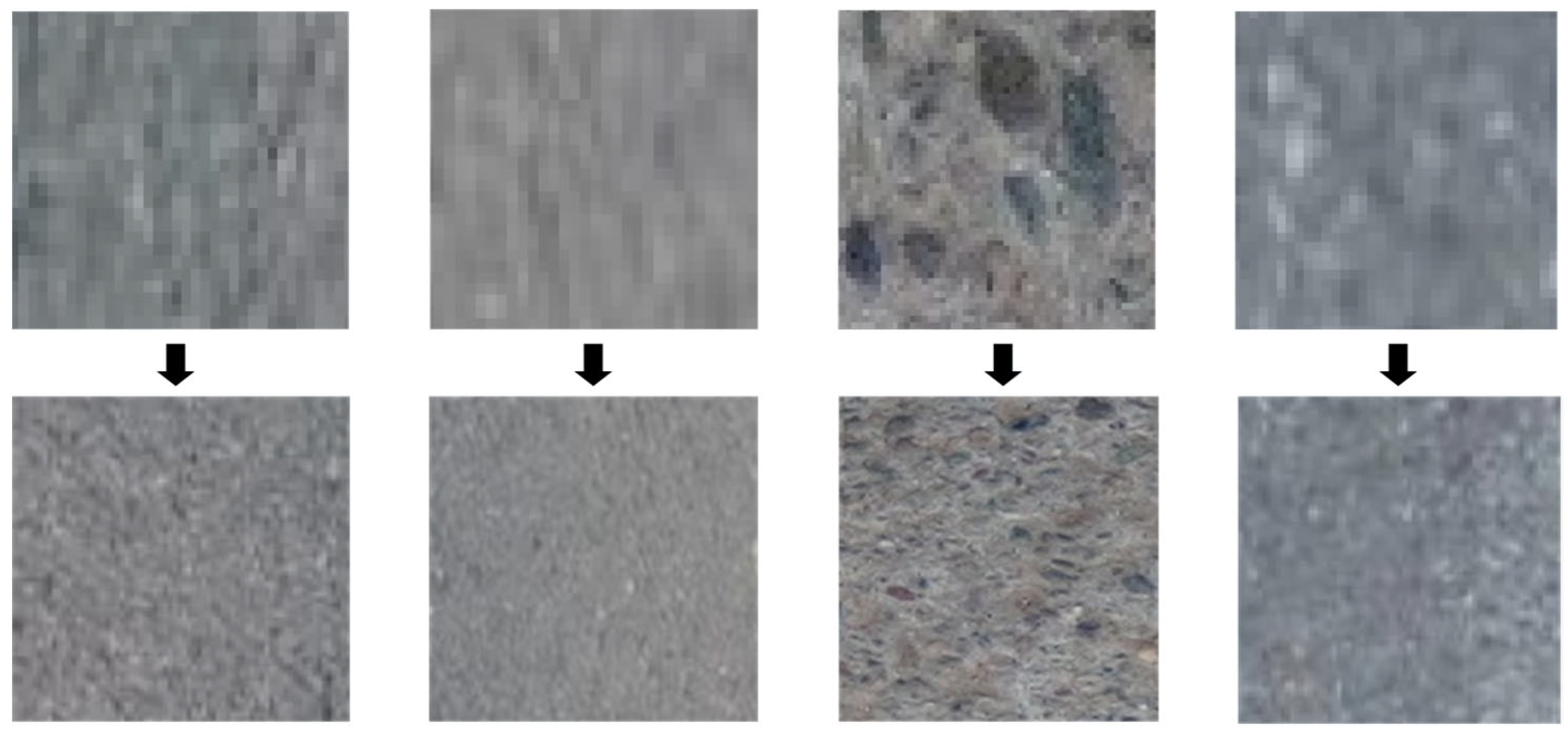
To solve this problem, this article adopts the bicubic interpolation algorithm in the decoder module of the U-Net network, as shown in Figure 10, which uses the weighted average of the 16 nearest neighboring pixels to compute the target pixel value, and the weighting coefficients are determined by the BiCubic basis function. Compared with the bilinear interpolation algorithm, the bicubic interpolation algorithm is more even in dealing with the pixels at the edges and can produce good results when zooming in and out of the image. When zooming in and out, the image can produce good results, and the comparison effect is shown in Figure 11.

4. Establish a Highway Crack Width Calculation Model

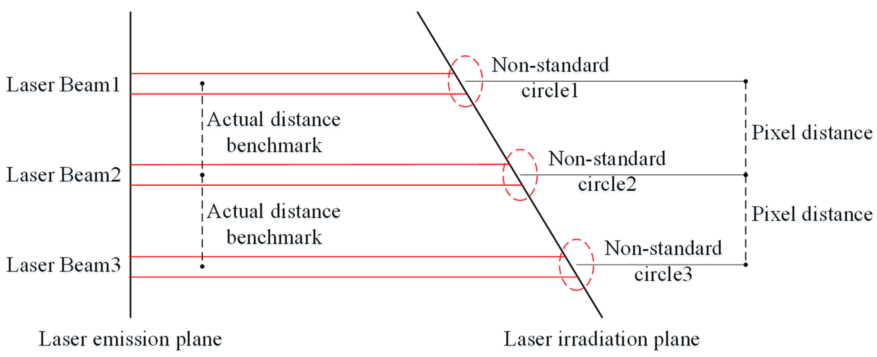
The crack width calculation method based on parallel laser beams solves the problem of the lack of measurement reference of the camera as a measurement tool, as shown in Figure 12, but the laser rays will show a asymmetric diffusion phenomenon in the process of use. The laser spot produces irregular deformation, which leads to inaccurate positioning of the center of the laser spot, and thus affects the accuracy of crack width calculation. In order to solve this problem, this article proposes a laser spot center positioning method based on the information entropy combination model. Firstly, the center coordinates of each laser spot in the image are calculated using the ellipse-fitting-based spot center positioning algorithm and the grayscale-gravity-based spot center positioning algorithm, respectively. Then, the weighting coefficients of the center positioning of each spot are determined by the information entropy combination model, and the final weighting results are taken as the actual center coordinates of each spot. The final weighted result is used as the actual center coordinates of each spot, thus reducing the crack width calculation error.

4.1. Laser Spot Center Localization Algorithm Based on Ellipse Fitting

Assuming the parameter equation of the ellipse is $a{x}^2+bxy+c{y}^2+dx+ey+1=0$, where $a,b,c,d,e$ are the coefficients of the parameter equation, let $p_{ij}(x_{ij},y_{ij})(i=\mathrm{1,2},3;j=1,2\dots .N,N\ge 5)$ be the j measurement point on the contour of ellipse i. To improve the accuracy of the calculation results, the number of measurement points N should be as large as possible. According to the principle of least squares, the fitted objective function is $f\left(a,b,c,d,e\right)={\sum }_{j=1}^N({a_i{x}_{ij}^2+b_i{x}_{ij}{y}_{ij}+c_i{y}_{ij}^2+d_i{x}_{ij}+e_i{y}_{ij}+1)}^2$.

Using the extreme value theorem to minimize the objective function, $f_i(a_i,b_i,c_i,d_i,e_i)$ is minimized, which can be obtained:

$${\displaystyle \frac{\partial f_i}{\delta a_i}}={\displaystyle \frac{\partial f_i}{\delta b_i}}={\displaystyle \frac{\partial f_i}{\delta c_i}}={\displaystyle \frac{\partial f_i}{\delta d_i}}={\displaystyle \frac{\partial f_i}{\delta e_i}}=0$$

(3)

Solving the above linear equation system, the values of $a_i,b_i,c_i,d_i,e_i$ can be obtained. Based on the geometric principles of ellipses, the coordinates of the center of the ellipse can be further computed ${(x}_{i0}{,y}_{i0})$, the semi-axis $A_i$, the short half-axis $B_i$ and the long axis inclination ${\theta }_i$, as shown in Formulas (4)–(8):

$$x_{i0}={\displaystyle \frac{2b_i{e}_i-c_i{d}_i}{4a_i{c}_i-b_i^2}}$$

(4)

$$y_{i0}={\displaystyle \frac{b_i{d}_i-{2a}_i{e}_i}{4a_i{c}_i-b_i^2}}$$

(5)

$$A_i=\sqrt{{\displaystyle \frac{2\left(a_i{x}_{i0}^2+c_i{y}_{i0}^2+b_i{x}_{i0}{y}_{i0}-1\right)}{a_i+c_i-\sqrt{{\left(a_i-c_i\right)}^2+b_i^2}}}}$$

(6)

$$B_i=\sqrt{{\displaystyle \frac{2\left(a_i{x}_{i0}^2+c_i{y}_{i0}^2+b_i{x}_{i0}{y}_{i0}-1\right)}{a_i+c_i+\sqrt{{\left(a_i-c_i\right)}^2+b_i^2}}}}$$

(7)

$${\theta }_i={\displaystyle \frac{1}{2}}{\tan }^{-1}{\displaystyle \frac{b_i}{a_i-c_i}}$$

(8)

After fitting the three ellipses corresponding to the three laser spots, we calculate the ellipse pixel center distance $P_{13}=P_{12}+P_{23}$, and then the actual pixel size is shown in Formula (9):

$$dp={\displaystyle \frac{1}{3}}\left({\displaystyle \frac{D_{12}}{P_{12}}}+{\displaystyle \frac{D_{23}}{P_{23}}}+{\displaystyle \frac{D_{13}}{P_{13}}}\right)$$

(9)

In practice, due to laser divergence, changes in light on the irradiated surface, etc., the semi-axes $A_i$, the short half-axis $B_i$ and long axis inclination ${\theta }_i$ fitted for the three ellipses may differ. In view of this problem, the following method is used to correct the fitted ellipses to reduce the error of spot center positioning due to ellipse fitting. We calculate the mean value of the sum of the squares of the errors corresponding to the data of each point of the three ellipses fitted and the original data of the spot edge, and the calculation is shown in Formula (10):

$${MSE}_i={\displaystyle \frac{1}{N}}\sum _{j=1}^N{\left(y_{ij-}\widehat{y_{ij}}\right)}^2$$

(10)

From the results of the calculation, we find the three ellipses in the MSE. The smallest one is set to m, and then the $A_i,B_i,{\theta }_i$ calculation is shown in Formula (11):

$$\left\{\begin{array}{c}{A}_i=A_m\\ B_i=B_m,i=1,2,3 i\ne m\\ {\theta }_i={\theta }_m\end{array}\right.$$

(11)

As $A_m,B_m,{\theta }_m$ is known, then for m two ellipses outside, it is only necessary to recompute the $a_i,b_i,c_i,d_i,e_i$. The two parameters in the center are sufficient.

4.2. Laser Spot Center Localization Algorithm Based on Grayscale Center of Gravity

The use of the ellipse fitting method for laser spot center localization is more suitable for images with clear boundaries, but in real operation, the boundaries of these images may be interfered with by a large amount of complex information, in which case, the use of other methods such as grayscale gravity can be considered in conjunction with the use of simultaneous processing.

Suppose that an image is of size $M pixel\times N pixel$, and the grayscale value of $I\left(i,j\right)$ at pixels $\left(i,j\right)$, and the coordinates of the center of the target pattern is $\left(x_0,y_0\right)$. The grayscale center of gravity is calculated as shown in Formula (12):

$$\left\{\begin{array}{c}{x}_0={\displaystyle \frac{{\sum }_{i=1}^M{\sum }_{j=1}^{N}I\left(i,j\right)\ast i}{{\sum }_{i=1}^M{\sum }_{j=1}^{N}I\left(i,j\right)}}\\ y_0={\displaystyle \frac{{\sum }_{i=1}^M{\sum }_{j=1}^{N}I\left(i,j\right)\ast j}{{\sum }_{i=1}^M{\sum }_{j=1}^{N}I\left(i,j\right)}}\end{array}\right.$$

(12)

The grayscale center of gravity method is simple to compute, faster, and the positioning accuracy is generally within 1 pixel. As all pixels of the spot are involved in the operation, it has less influence on single-point noise, but the grayscale center of gravity method can only deal with the situation where the shape of the target pattern is more regular and the grayscale distribution is more uniform.

4.3. Laser Spot Center Localization Algorithm Based on Information Entropy Combination Model

Let three laser spot centers $\left(x_{i0},y_{i0}\right),i=1,2,3$, respectively. Using the ellipse fitting method and the grayscale center of gravity method above to locate their spot centers, the m method is used to locate the spot centers of the i, and the calculated value of the spot center is $\left(x_{im},y_{im}\right).$ Let the value of $e_{im}$ be the error of the m method for the spot centers of i, and the $e_{im}$ is shown in Formula (13):

$$e_{im}=\left\{\begin{array}{c}1 + {\displaystyle \frac{\sqrt{{\left(x_{i0}-x_{im}\right)}^2+{\left(y_{i0}-y_{im}\right)}^2}}{\sqrt{x_{i0}^2+y_{i0}^2}}}\ge 1\\ {\displaystyle \frac{\sqrt{{\left(x_{i0}-x_{im}\right)}^2+{\left(y_{i0}-y_{im}\right)}^2}}{\sqrt{x_{i0}^2+y_{i0}^2}}} + {\displaystyle \frac{\sqrt{{\left(x_{i0}-x_{im}\right)}^2+{\left(y_{i0}-y_{im}\right)}^2}}{\sqrt{x_{i0}^2+y_{i0}^2}}}<1\end{array}\right.$$

(13)

The relative errors of the two spot center calculation methods are normalized, as shown in Formulas (14) and (15):

$$p_{im}={\displaystyle \frac{e_{im}}{{\sum }_{i=1}^3{e}_{im}}}i=1,2,3$$

(14)

$$\sum _1^3{p}_{im}=1$$

(15)

The calculation of the relative error entropy hmhm of the m laser spot calculation method, with the scaling factor k ≥ 0, is given in Formula (16).

$$h_m=-k\sum _{i=1}^3{p}_{im}\ln p_{im}m=1,2$$

(16)

The weighting factors for the two calculation methods $l_m(m=1,2)$ are shown in Formula (17):

$$l_m=1-{\displaystyle \frac{1-h_m}{{\sum }_{m=1}^2\left(1-h_m\right)}}$$

(17)

The final combination method for calculating the spot center is shown in Formula (18):

$$\left\{\begin{array}{c}\widehat{x_{i0}}={\displaystyle \sum _{m=1}^2}{l}_m{x}_{im}\\ \widehat{y_{i0}}={\displaystyle \sum _{m=1}^2}{l}_m{y}_{im}\end{array}i=1,2,3\right.$$

(18)

5. Experimental Validation

The experimental hardware and software environment is as follows: Central Processing Unit, Intel core i7-12400KF; Graphics Processing Unit, NVIDIA GeForce RTX 3060Ti; Operating System, Windows11; Integrated Development Environment, Pycharm.

We used the Labelimg image labeling tool to create a crack detection dataset consisting of 1528 images, divided into training and validation sets in a 4:1 ratio. Each training batch contains 16 images, with an initial learning rate of 0.1, a cyclic learning rate of 0.01, and a maximum total training epochs of 900. The optimal training parameters are generated based on minimizing the loss function value.

We used the Labelme image labeling tool to create a crack segmentation dataset, consisting of 1008 images, divided into training and validation sets in a 4:1 ratio. Each training batch contains 16 images, with an initial learning rate of 0.1, a cyclic learning rate of 0.01, and a maximum total training epochs of 90. The optimal training parameters are generated based on minimizing the loss function value.

5.1. Analysis of Crack Detection Results

5.1.1. Numerical Analysis

In this article, the effectiveness of the proposed crack detection network is evaluated in terms of precision (Pre), recall (Rec), and mean average precision (mAP), as shown in Formulas (19)–(21). Pre represents the percentage of true positive samples in all samples predicted as positive; Rec represents the proportion of true positive samples accurately identified and detected among all true positive samples; mAP is a metric that evaluates the overall performance of a network considering the impact of different intersection over union (IoU). Additionally, compared with the existing Yolov5-s network and Yolov5-mobileone network, the experimental results are shown in

Table 1. Comparison of evaluation indicators for detection networks.

Network	Pre	Rec	mAP0.5	mAP0.5:0.95
Yolov5-s	0.958 (+1.3%)	0.930 (+5.0%)	0.971 (+1.8%)	0.703 (+10.2%)
Yolov5-mobileone	0.875 (+9.6%)	0.866 (+9.4%)	0.887 (+10.2%)	0.601 (+22.2%)
CFSSE	0.971	0.980	0.989	0.823

, and the CFSSE network improved in all aspects.

$$\mathit{Pre}={\displaystyle \frac{TP}{TP+FP}}$$

(19)

$$Rec={\displaystyle \frac{TP}{TP+FN}}$$

(20)

$$mAP={\displaystyle \frac{1}{N_{cls}}}\sum _{i}A{P}_i$$

(21)

5.1.2. Visual Analysis

To further validate the effectiveness of the proposed CFSSE network applied to crack detection, this article presents a series of graph of crack detection results to visually compare the differences between each network, including the detection results of transverse cracks, longitudinal cracks, diagonal cracks, mesh cracks, and cracks under insufficient light conditions.

In the detection experiments of transverse cracks, as shown in Figure 13, the Yolov5-mobileone network shows leakage detection of cracks, the Yolov5-s network detects too many cracks, and the confidence level of the cracks detected by both is low. The CFSSE network in this paper achieves accurate detection of cracks, while the confidence level is higher than that of the Yolov5-mobileone model and the Yolov5-s model.

In the detection experiments of longitudinal cracks, as shown in Figure 14, the Yolov5-mobileone network did not detect all the cracks, and the Yolov5-s network appeared to overlap the crack inspections. The CFSSE network basically realized the detection of each crack and did not appear to overlap the inspection frames.

In the diagonal crack detection experiments, as shown in Figure 15, all the cracks in the image were detected by each network, but the Yolov5-mobileone network and the Yolov5-s network were poorly detected relative to the CFSSE network in this article, with incomplete coverage of crack detection and lower confidence than the CFSSE network.

In the detection experiments of mesh cracks, as shown in Figure 16, the Yolov5-mobileone network and Yolov5-s network showed leakage and did not detect all the cracks, and the CFSSE network in this article detected all the cracks with higher confidence than all the other networks.

In the crack detection experiments under insufficient light conditions, as shown in Figure 17, both the Yolov5-mobileone network and the Yolov5-s network showed poor detection results due to overlapping crack detection results caused by insufficient light conditions. The CFSSE network proposed in this paper does not show any overlapping detection of cracks due to insufficient light.

5.2. Analysis of Crack Segmentation Results

5.2.1. Numerical Analysis

In this article, the effectiveness of the proposed crack segmentation network is evaluated in terms of average accuracy (ACC), mean pixel accuracy (MPA), and mean intersection over union (MIoU), as shown in Formulas (22)–(24). ACC represents the ratio of correctly predicted samples to the total predicted samples; MPA represents the proportion of correctly predicted category pixels to the total number of pixels; MIoU represents the intersection of predicted and actual regions divided by the union of predicted and actual regions. Additionally, compared with the original U-Net network, the original Deeplab V3+ network, and the optimized Deeplab V3 network, the experimental results are shown in

Table 2. Comparison of evaluation indicators for segmentation networks.

Network	ACC	MPA	MIoU
U-Net	0.9679 (+2.31%)	0.9314 (+0.22%)	0.7510 (+13.52%)
DeeplabV3+	0.9898 (+0.12%)	0.9340 (+0.16%)	0.8747 (+1.15%)
Optimized DeeplabV3	0.9903 (+0.07%)	0.9328 (+0.28%)	0.8810 (+0.52%)
CBU-Net	0.9910	0.9356	0.8862

. CBU_Net network improved in all aspects.

$$ACC={\displaystyle \frac{TP+TN}{TP+FP+TN+FN}}$$

(22)

$$MPA={\displaystyle \frac{1}{k+1}}\sum _{i=0}^k{\displaystyle \frac{{TP}_i}{T{P}_i+F{N}_i}}$$

(23)

$$MIoU={\displaystyle \frac{1}{k+1}}\sum _{i=0}^k{\displaystyle \frac{TP}{FN+FP+TP}}$$

(24)

5.2.2. Visual Analysis

To further validate the effectiveness of the proposed CBU-Net network applied to crack segmentation, this article presents crack segmentation result plots to visually compare the differences between the individual networks, including the detection results of transverse cracks, longitudinal cracks, diagonal cracks, mesh cracks, and cracks under insufficient light conditions.

In the transverse crack segmentation experiments, as shown as Figure 18, all other segmentation networks showed fractured segmentation of the fine edges of the cracks, while the CBU-Net network segmented the transverse cracks accurately, and there was no fractured segmentation of the cracks.

In the longitudinal crack segmentation experiments, as shown in Figure 19, other networks showed that fine cracks appeared to be missed or incompletely segmented, while the CBU-Net network achieved accurate segmentation of micro-fine cracks.

In the diagonal crack segmentation experiments, as shown in Figure 20, at the crack junction, other networks have crack segmentation breaks, while the CBU-Net network achieves a complete segmentation of the cracks.

In the mesh crack segmentation experiments, as shown in Figure 21, other segmentation networks have crack segmentation breaks and the crack profile is not segmented completely, while the CBU-Net network accomplishes accurate segmentation of the entire crack network without breaks.

In the crack segmentation experiments under insufficient light conditions, as shown in Figure 22, the U-Net segmentation network showed two fine crack segmentations and the segmentation width of the cracks was slightly larger than the other segmentation networks, while the DeeplabV3+ network and the optimized DeeplabV3 network showed two cracks segmentation breaks, and the CBU-Net network segmentation results were more complete.

5.3. Analysis of Crack Width Calculation Results

5.3.1. Visual Analysis

In this article, the following five images containing cracks and laser spots are selected to repeat the experiment, as shown in Figure 23, respectively, using the method based on ellipse fitting, the method based on grayscale gravity, and the method based on the combination of information entropy to calculate the center coordinates of each spot within the image and then calculate the width of the crack. In order to save space, this article only provides the first image as an example to show the effect of different methods of spot center localization, as shown in Figure 24.

5.3.2. Numerical Analysis

Crack Width Calculation Experiment I results are shown in

Table 3. Crack width calculation experiment I.

	Ellipse Fitting	Grayscale Centroid	Information Entropy
Circle 1	(699.5, 362.5)	(699.0, 362.5)	(699.405, 362.500)
Circle 2	(698.5, 713.5)	(698.5, 713.0)	(698.500, 713.215)
Circle 3	(699.5, 1134.5)	(699.0, 1134.0)	(699.405, 1134.420)

. The average distance between the light spots is 385.979 pixels, and according to the actual physical distance between the centers of the light spots it is 5 cm. The actual physical distance represented by the unit pixel is 0.014 cm, the width of the crack is 3.54 pixel units, and the actual width of the crack is 0.050 cm.

Crack Width Calculation Experiment II results are shown in

Table 4. Crack width calculation experiment II.

	Ellipse Fitting	Grayscale Centroid	Information Entropy
Circle 1	(263.5, 805.5)	(263.0, 806.5)	(263.120, 805.650)
Circle 2	(729.5, 804.5)	(729.5, 804.0)	(729.500, 804.120)
Circle 3	(1195.5, 805.5)	(1195.5, 806.0)	(1195.500, 805.800)

. The average distance between the light spots is 425.311 pixels, and according to the actual physical distance between the centers of the light spots it is 5 cm. The actual physical distance represented by the unit pixel is 0.012 cm, the width of the crack is 27.17 pixel units, and the actual width of the crack is 0.319 cm.

Crack Width Calculation Experiment III results are shown in

Table 5. Crack width calculation experiment III.

	Ellipse Fitting	Grayscale Centroid	Information Entropy
Circle 1	(300.5, 489.5)	(300.0, 490.5)	(300.120, 489.650)
Circle 2	(766.5, 489.5)	(766.5, 490.0)	(766.690, 489.620)
Circle 3	(1232.5, 489.5)	(1232.5, 490.0)	(1232.890, 489.800)

. The average distance between the light spots is 466.193 pixels, and according to the actual physical distance between the centers of the light spots it is 5 cm. The actual physical distance represented by the unit pixel is 0.012 cm, the crack is 2.74 pixel units, and the actual width of the crack is 0.029 cm.

Crack Width Calculation Experiment IV results are shown in

Table 6. Crack width calculation experiment IV.

	Ellipse Fitting	Grayscale Centroid	Information Entropy
Circle 1	(201.5, 637.5)	(201.0, 637.0)	(201.240, 637.240)
Circle 2	(769.5, 637.5)	(771.0, 637.0)	(770.770, 637.230)
Circle 3	(1338.5, 637.5)	(1339.0, 637.0)	(1338.770, 637.230)

. The average distance between the light spots is 568.765 pixels, and according to the actual physical distance between the centers of the light spots it is 5 cm. The actual physical distance represented by the unit pixel is 0.009 cm, the width of the crack is 4.90 pixel units, and the actual width of the crack is 0.043 cm.

Crack Width Calculation Experiment V result are shown in

Table 7. Crack width calculation experiment V.

	Ellipse Fitting	Grayscale Centroid	Information Entropy
Circle 1	(111.5, 1186.5)	(111.0, 1186.5)	(111.360, 1186.230)
Circle 2	(689.5, 1186.5)	(689.0, 1186.5)	(689.390, 1186.500)
Circle 3	(1149.5, 1186.5)	(1150.5, 1186.5)	(1149.770, 1186.500)

. The average distance between the light spots is 519.205 pixels, and according to the actual physical distance between the centers of the light spots it its 5 cm. The actual physical distance represented by the unit pixel is 0.01 cm, the width of the crack is 8.19 pixel units, and the actual width of the crack is 0.079 cm.

From

Table 8. Comparison of crack width calculation accuracy.

	Crack 1	Crack 2	Crack 3	Crack 4	Crack 5
Calculate Width	0.50 mm	3.19 mm	0.29 mm	0.43 mm	0.79 mm
Actual Width	0.48 mm	3.21 mm	0.30 mm	0.44 mm	0.77 mm
Error	0.02 mm	0.02 mm	0.01 mm	0.01 mm	0.02 mm
	(4.0%)	(0.6%)	(3.4%)	(2.3%)	(2.5%)
Mean Error	2.56%
Reference [24]	4.00% (−1.44%)

, it can be seen that the average error of the crack width calculation method based on the combined information entropy model proposed in this article is 2.56% (compared with the 4.00% error of Reference [24]). The method proposed in this article is effective, and the calculated crack widths are closer to the real values.

6. Conclusions and Future Work

Firstly, the CFSSE network proposed in this article achieves rapid and accurate identification and positioning of highway cracks, greatly improving the previous situations of false alarms or missed detections, laying a good foundation for subsequent crack segmentation work. Secondly, the CBU-Net network proposed in this article achieves precise segmentation of highway cracks, especially optimizing the segmentation of small cracks and the handling of crack edges. Furthermore, the information entropy combination method proposed in this article achieves precise positioning of the center of irregular laser spots, and then accurately calculates the crack width. Finally, based on digital image processing, this article integrates road crack detection, segmentation, and width calculation, enhancing the scientific and refined level of highway preventive maintenance.

This article conducted multiple experiments on the proposed crack detection network and segmentation network on the selected dataset, proving the effectiveness and reliability of the improvements. However, there are still the following issues that need further research:

(1)

During the training process of the crack detection network, the use of Generative Adversarial Networks (GANs) can be explored to augment the dataset with complex crack images, further enhancing the applicability of the crack detection network.

(2)

In the process of annotating crack images for the segmentation dataset, designing an automatic crack image annotation tool can improve the efficiency of creating crack segmentation datasets.

References

- Jiang, Y.Q.; Pang, D.D.; Li, C.D. A Deep Learning Approach for Fast Detection and Classification of Concrete Damage. Autom. Constr. 2021, 128, 103785. [Google Scholar] [CrossRef]
- Hu, G.X.; Hu, B.L.; Yang, Z.; Huang, L.; Li, P. Pavement Crack Detection Method Based on Deep Learning Models. Wirel. Commun. Mob. Comput. 2021, 8, 1–13. [Google Scholar]
- Ma, D.; Fang, H.; Wang, N.; Zhang, C.; Dong, J.; Hu, H. Automatic Detection and Counting System for Pavement Cracks Based on PCGAN and YOLO-MF. IEEE Trans. Intell. Transp. Syst. 2022, 23, 22166–22178. [Google Scholar] [CrossRef]
- Hu, N.; Yang, J.J.; Jin, X.C.; Fan, X.L. Few-Shot Crack Detection Based on Image Processing and Improved YOLOv5. J. Civ. Struct. Health Monit. 2023, 13, 165–180. [Google Scholar] [CrossRef]
- Song, W.D.; Jia, G.H.; Zhu, H.; Gao, L. Automated Pavement Crack Damage Detection Using Deep Multiscale Convolutional Features. J. Adv. Transp. 2020, 2020, 6412562. [Google Scholar] [CrossRef]
- Ibragimov, E.; Lee, H.J.; Lee, J.J.; Kim, N. Automated Pavement Distress Detection Using Region-Based Convolutional Neural Networks. Int. J. Pavement Eng. 2022, 23, 1981–1992. [Google Scholar]
- Chaiyasarn, K.; Buatik, A.; Mohamad, H.; Zhou, M.L.; Kongsilp, S.; Poovarodom, N. Integrated Pixel-level CNN-FCN Crack Detection Via Photogrammetric 3D Texture Mapping of Concrete Structures. Autom. Constr. 2022, 140, 104388. [Google Scholar] [CrossRef]
- Chen, C.; Seo, H.; Zhao, Y. A Novel Pavement Transverse Cracks Detection Model Using WT-CNN and STFT-CNN for Smartphone Data Analysis. Int. J. Pavement Eng. 2022, 23, 4372–4384. [Google Scholar]
- Gan, L.F.; Liu, H.; Yan, Y.; Chen, A.R. Bridge Bottom Crack Detection and Modeling Based on Faster R-CNN and BIM. IET Image Process. 2024, 18, 664–677. [Google Scholar] [CrossRef]
- Tran, V.P.; Tran, T.S.; Lee, H.J.; Kim, K.D.; Baek, J.; Nguyen, T.T. One-Stage Detector (RetinaNet)-Based Crack Detection for Asphalt Pavements Considering Pavement Distresses and Surface Objects. J. Civ. Struct. Health Monit. 2021, 11, 205–222. [Google Scholar]
- Guo, F.; Qian, Y.; Liu, J.; Yu, H.Y. Pavement Crack Detection Based on Transformer Network. Autom. Constr. 2023, 145, 104646. [Google Scholar] [CrossRef]
- Wang, C.; Liu, H.B.; An, X.Y.; Gong, Z.Q.; Deng, F. SwinCrack: Pavement Crack Detection Using Convolutional Swin-transformer Network. Digit. Signal Process. 2024, 145, 104297. [Google Scholar] [CrossRef]
- Cui, X.N.; Wang, Q.C.; Dai, J.P.; Xue, Y.J.; Duan, Y. Intelligent Crack Detection Based on Attention Mechanism in Convolution Neural Network. Adv. Struct. Eng. 2021, 24, 1859–1868. [Google Scholar] [CrossRef]
- Yang, Y.L.; Zhao, Z.H.; Su, L.L.; Zhou, Y.; Li, H. Research on Pavement Crack Detection Algorithm Based on Deep Residual Unet Neural Network. J. Phys. Conf. Ser. 2022, 2278, 012020. [Google Scholar] [CrossRef]
- Xu, N.; He, L.Z.; Li, Q. Crack-Att Net: Crack Detection Based on Improved U-Net with Parallel Attention. Multimed. Tools Appl. 2023, 82, 42465–42484. [Google Scholar] [CrossRef]
- Ronneberger, O.; Fischer, P.; Brox, T. U-Net: Convolutional Networks for Biomedical Image Segmentation. Med. Image Comput. Comput.-Assist. Interv. 2015, 1505, 234–241. [Google Scholar]
- Zou, Q.; Zhang, Z.; Li, Q.Q.; Qi, X.B.; Wang, Q.; Wang, S. DeepCrack: Learning Hierarchical Convolutional Features for Crack Detection. IEEE Trans. Image Process. A Publ. IEEE Signal Process. Soc. 2019, 28, 1498–1512. [Google Scholar] [CrossRef]
- Chen, T.Y.; Cai, Z.H.; Zhao, X.; Chen, C.; Liang, X.F.; Zou, T.R.; Wang, P. Pavement Crack Detection and Recognition Using the Architecture of SegNet. J. Ind. Inf. Integr. 2020, 18, 100144. [Google Scholar] [CrossRef]
- Mei, Q.; Gül, M. A Cost Effective Solution for Pavement Crack Inspection Using Cameras and Deep Neural Networks. Constr. Build. Mater. 2020, 256, 119397. [Google Scholar] [CrossRef]
- Badrinarayanan, V.; Kendall, A.; Cipolla, R. SegNet: A Deep Convolutional Encoder Decoder Architecture for Image Segmentation. IEEE Trans. Pattern Anal. Mach. Intell. 2017, 39, 2481–2495. [Google Scholar] [CrossRef]
- Chen, L.C.; Papandreou, G.; Kokkinos, I.; Murphy, K.; Yuille, A.L. DeepLab: Semantic Image Segmentation with Deep Convolutional Nets, Atrous Convolution, and Fully Connected CRFs. IEEE Trans. Pattern Anal. Mach. Intell. 2018, 40, 834–848. [Google Scholar]
- Ji, A.K.; Xue, X.L.; Wang, Y.N.; Luo, X.W.; Xue, W.R. An Integrated Approach to Automatic Pixel-Level Crack Detection and Quantification of Asphalt Pavement. Autom. Constr. 2020, 114, 103176. [Google Scholar] [CrossRef]
- Zhou, Z.; Zheng, Y.D.; Zhang, J.J.; Yang, H. Fast Detection Algorithm for Cracks on Tunnel Linings Based on Deep Semantic Segmentation. Front. Struct. Civ. Eng. 2023, 17, 732–744. [Google Scholar] [CrossRef]
- Weng, X.X.; Huang, Y.C.; Wang, W.Z. Segment-based pavement crack quantification. Autom. Constr. 2019, 105, 102819. [Google Scholar] [CrossRef]
- Chen, J.; Yuan, Y.; Lang, H.; Lu, J.J. The Improvement of Automated Crack Segmentation on Concrete Pavement with Graph Network. J. Adv. Transp. 2022, 2022, 2238095. [Google Scholar] [CrossRef]
- Yang, K.; Ding, Y.L.; Sun, P.; Jiang, H.C.; Wang, Z.W. Computer Vision Based Crack Width Identification Using F-CNN Model and Pixel Nonlinear Calibration. Struct. Infrastruct. Eng. 2023, 19, 978–989. [Google Scholar]
Figure 1.
CFSSE highway crack detection network structure.
Figure 2.
Fast spatial pyramid pooling structure.
Figure 3.
Schematic diagram of convolution operation.
Figure 4.
Squeeze–excitation attention mechanism structure.
Figure 5.
CBU_Net highway crack segmentation network structure.
Figure 6.
CBU_Net highway crack segmentation network encoder module.
Figure 7.
Dropout operation.
Figure 8.
Activation function: (a) ReLU activation function; (b) frontal activation function with leakage-corrected linear unit.
Figure 9.
Checkerboard effect.
Figure 10.
Bicubic interpolation algorithm.
Figure 11.
The chessboard effect through bicubic interpolation.
Figure 12.
Calculation method of crack width based on parallel laser.
Figure 13.
Transverse crack detection comparison result.
Figure 14.
Longitudinal crack detection comparison result.
Figure 15.
Diagonal crack detection comparison result.
Figure 16.
Mesh crack detection comparison result.
Figure 17.
Crack detection under low light condition comparison result.
Figure 18.
Transverse crack segmentation comparison result.
Figure 19.
Longitudinal crack segmentation comparison result.
Figure 20.
Diagonal crack segmentation comparison result.
Figure 21.
Mesh crack segmentation comparison result.
Figure 22.
Crack segmentation under low light condition comparison result.
Figure 23.
Experimental image of crack width calculation.
Figure 24.
Laser spot center position: (a) is the ellipse fitting method, (b) is the grayscale centroid method, and (c) is the information entropy method.