Article

An Improved Comprehensive Learning Jaya Algorithm with Lévy Flight for Engineering Design Optimization Problems

1
College of Computing, Khon Kaen University, Khon Kaen 40002, Thailand
2
School of Computer Science and Information Security, Guilin University of Electronic Technology, Guilin 541000, China
*
Author to whom correspondence should be addressed.
Electronics 2025, 14(19), 3776; https://doi.org/10.3390/electronics14193776
Submission received: 13 August 2025 / Revised: 13 September 2025 / Accepted: 15 September 2025 / Published: 24 September 2025

Abstract

The JAYA algorithm has been widely applied due to its simplicity and efficiency but is prone to entrapment in sub-optimal solutions. This study introduces the Lévy flight mechanism and proposes the CLJAYA-LF algorithm, which integrates large-step and small-step Lévy movements with a multi-strategy particle update mechanism. The large-step strategy enhances global exploration and helps escape local optima, while the small-step strategy improves fine-grained local search accuracy. Extensive experiments on the CEC2017 benchmark suite and real-world engineering optimization problems demonstrate the effectiveness of CLJAYA-LF. In 50-dimensional benchmark problems, it outperforms JAYA, JAYALF, and CLJAYA in 15 of 22 functions with lower mean fitness and competitive variance; in 100-dimensional problems, it achieves smaller variance in 17 of 24 functions. For engineering applications, CLJAYA-LF attains a mean of 16.9 and variance of 0.332 for the Step-cone Pulley, 1.44 × 10⁻¹⁵ and 3.14 × 10⁻¹⁵ for the Gear Train, and 0.535 and 0.0498 for the Planetary Gear Train, surpassing most JAYA variants. These results indicate that CLJAYA-LF delivers superior optimization performance while maintaining robust stability across dimensions and problem types, demonstrating significant potential for complex and high-dimensional optimization scenarios.

1. Introduction

Optimization techniques play a crucial role in today’s rapidly advancing technological era, with applications spanning engineering, healthcare, transportation, energy systems, and financial modeling. These methods improve efficiency, reduce costs, and enhance system performance. As the demand for optimization continues to grow, optimization algorithms have become a central focus in both academic research and industrial applications [1].
Traditional optimization methods, such as linear programming [2], dynamic programming [3], and gradient-based approaches [4], perform well for structured, low-dimensional, and convex problems. However, they face significant challenges when applied to complex real-world scenarios, which often feature multimodal landscapes with numerous local optima, high dimensionality, and nonlinear or discontinuous objective functions. Moreover, dynamic and stochastic environments, such as traffic systems and financial markets, add further complexity. These limitations highlight the need for novel approaches capable of effectively handling complex optimization tasks.
Nature-inspired algorithms have emerged to address these challenges, particularly excelling in large-scale, multimodal, and complex optimization problems [5,6]. These algorithms are valued for their simplicity, robust global search capabilities, and adaptability. Their core principle is to simulate natural laws or scientific phenomena, integrating randomized search with heuristic strategies to explore vast solution spaces efficiently while balancing global exploration and local exploitation.
Among evolutionary mechanism-based algorithms, the Genetic Algorithm (GA) [4,5,6] simulates natural selection and genetic variation to optimize objective functions, performing well on small- to medium-scale problems but prone to local optima in high-dimensional complex tasks. Evolution Strategies (ES) [7] emphasize individual variation and survival-of-the-fittest principles, improving robustness in complex landscapes. Differential Evolution (DE) [8,9] utilizes differences among individuals to guide optimization, achieving notable performance in continuous spaces. The recently proposed Alpha Evolution Algorithm [10,11] introduces adaptive evolution strategies to dynamically adjust search directions. The Beetle Antennae Search (BAS) [12] mimics beetle foraging behavior, offering simple yet effective global search but relatively slower convergence. While each algorithm has its strengths, single evolutionary algorithms may struggle to balance exploration and exploitation in high-dimensional multimodal problems, motivating the development of multi-strategy enhancements.
In swarm intelligence algorithms, Particle Swarm Optimization (PSO) [13,14,15] mimics bird flock foraging, combining simplicity and fast convergence, though it is prone to premature convergence. Artificial Bee Colony (ABC) [16] models collaborative foraging behavior to improve information sharing and solution quality. Grey Wolf Optimizer (GWO) [17] simulates wolf pack dynamics, enhancing global search through hierarchical guidance and cooperation. Algorithms such as Harris Hawks Optimization (HHO) [18] and Dwarf Mongoose Optimization (DMO) [19] utilize predatory or social behaviors to improve exploration in complex problems. The Egret Swarm Optimization Algorithm (ESOA) [20] combines sit-and-wait and aggressive strategies for efficient global search, demonstrating strong convergence and stability. PSO converges quickly but is susceptible to local optima, ABC exploits population information effectively but may lack local refinement, and GWO or HHO improve global exploration at the cost of increased computational complexity. This motivates hybrid or multi-strategy algorithms to balance efficiency, diversity, and convergence.
Human-inspired algorithms, including HEOA [21], TLBO [22,23], and HOA [24], simulate human learning, knowledge sharing, and decision-making, exhibiting strong adaptability in dynamic environments. The CTCM algorithm [25] models inter-tribal competition and intra-tribal cooperation, surpassing many advanced metaheuristics in convergence speed, stability, and global search capability.
Physics-inspired algorithms, such as Simulated Annealing [26], Water Flow Optimizer [27], Fick Law Algorithm (FLA) [28], and SABO [29], offer alternative search strategies by simulating natural or physical processes. These approaches are effective for certain constrained and continuous-space problems but often exhibit limited stability in high-dimensional nonlinear scenarios.
Despite these advances, most existing methods require careful parameter tuning, are sensitive to initial solutions, and are prone to local optima. The JAYA algorithm [30,31] mitigates some of these issues by using only the best and worst individuals to guide search, avoiding extra parameter settings. Nevertheless, JAYA can still reduce population diversity if the best individual is trapped in a local optimum. To address this, JAYA-LF [32] incorporates Lévy Flight-based random perturbations, and CLJAYA [33] employs multi-strategy learning to improve population information usage and search efficiency.
Building on these developments, this study proposes the CLJAYA-LF algorithm, which combines CLJAYA’s multi-strategy update mechanism with Lévy Flight’s large- and small-step perturbations. By preserving the guiding roles of the best and worst individuals, it overcomes the drawbacks of previous approaches, significantly enhancing the overall performance. The algorithm is evaluated on CEC2017 benchmark functions and real-world engineering optimization problems, demonstrating superior performance in both low- and high-dimensional tasks, validating its effectiveness and applicability in complex optimization scenarios. The main contributions of this work are summarized as follows:
  • Integration of Lévy Flights into the CLJAYA Framework Lévy Flights are seamlessly incorporated into the CLJAYA framework. This integration effectively enriches the diversity of particles and significantly boosts both the exploration and exploitation capabilities of the algorithm.
  • Enhanced global exploration: Using the large-step movement strategy of Lévy Flights, the CLJAYA-LF algorithm empowers particles to break free from local optima. Consequently, it substantially enhances the algorithm’s global exploration ability and effectively averts premature convergence towards suboptimal solutions.
  • Improved Local Exploitation: The algorithm synergistically combines the small-step random movement strategy of Lévy Flights to strengthen local exploitation. This combination effectively tackles the problem where particles face a restricted search area when approaching the optimal and worst solutions.
  • Superior Performance Evaluation: Through rigorous testing with the CEC 2017 benchmark suite, CLJAYA-LF demonstrates exceptional performance, surpassing existing advanced optimization methods. The results validate its effectiveness and robustness in both low- and high-dimensional optimization tasks.
The structure of the paper is as follows. Section 2 offers a concise introduction to the relevant works for this paper. Section 3 explains the proposed CLJAYA-LF. Section 4 presents the applications of CLJAYA-LF in numerical optimization. Section 5 presents the applications of CLJAYA-LF in engineering optimization. Finally, Section 6 draws conclusions from the research findings and results.

2. Related Works

2.1. CLJAYA Algorithm

The JAYA algorithm requires only two parameters, population size N and maximum number of iterations I t m a x , to adjust the position of each solution in the search space, gradually guiding it towards the optimal solution. During the update process, each solution is encouraged to move away from the current worst solution and towards the best solution found so far. This update process can be expressed by the following equation:
X i , j k + 1 = X i , j k + θ 1 ( X best , j k | X i , j k | ) θ 2 ( X worst , j k | X i , j k | ) ,
where k denotes the iteration number of the algorithm. X i , j k represents the j-th variable of the i-th particle. X best , j k is the j-th variable of the best solution, and X worst , j k is the j-th variable of the worst solution. Furthermore, X i , j k + 1 is the updated value of the variable j-th for the k + 1 iteration. The parameters θ 1 and θ 2 are random variables generated from a uniform distribution U ( 0 , 1 ) .
Although the JAYA algorithm is intuitively simple, it relies on a single learning strategy and does not fully utilize the information from the entire population. If the best particle becomes trapped in a local optimum, other particles may also be drawn into this local optimum, thereby reducing population diversity and hindering the ability to escape from local optima. To address this limitation, the Comprehensive Learning JAYA Algorithm (CLJAYA) introduces three distinct learning strategies to enhance particle diversity and improve the algorithm’s search efficiency. The update rule for CLJAYA [33] is shown in (2) and (3). For these equations, ϕ 1 , ϕ 2 , ϕ 3 and ϕ 4 follow the normal distribution. ϕ 5 , and ϕ 6 follow the uniform distribution U ( 0 , 1 ) . X best , j represents the value of the j-th variable in the best individual currently. X worst , j denotes the value of the variable j in the worst individual. M is the mean position of the current population, p and q are random integers with p q i , and p switch is a random variable that follows a uniform distribution U ( 0 , 1 ) .
X i , j k + 1 = X i , j k + ϕ 1 ( X best , j k     | X i , j k | )     ϕ 2 ( X worst , j k     | X i , j k | ) , if 0 p switch 1 3 , X i , j k + ϕ 3 ( X best , j k     | X i , j k | ) ϕ 4 ( M     | X i , j k | ) , if 1 3 < p switch 2 3 , X i , j k + ϕ 5 ( X best , j k     X i , j k ) + ϕ 6 ( X p , j k     X q , j k ) , if 2 3 < p switch 1 ,
and
M = 1 N i = 1 N X i .

2.2. Lévy Flight

Lévy Flight is a non-Gaussian random walk characterized by frequent small steps and occasional long jumps [34,35]. In the early stages of the search process, large step sizes allow the population to broadly explore the solution space, thereby improving the likelihood of escaping local optima and reducing the risk of premature convergence. In contrast, in the later stages, smaller steps facilitate refined exploitation near promising regions, leading to more effective convergence toward the global optimum. As a result, Lévy Flight has been widely integrated into metaheuristic algorithms [36,37,38].
The probability density function (PDF) of the Lévy distribution can be expressed as
L ( γ ) = s γ , 1 < γ 3 ,
where s denotes the step length, and γ is the stability parameter controlling the tail heaviness of the distribution. Smaller values of γ favor long jumps, while larger values result in more local steps.
The step length s is typically represented as
s = μ | ν | 1 / γ ,
where μ N ( 0 , σ μ 2 ) and ν N ( 0 , 1 ) are random variables sampled from normal distributions. The scaling parameter σ μ ensures the Lévy distribution satisfies its stability condition and is defined as
σ μ = Γ ( 1 + γ ) · sin π γ 2 Γ 1 + γ 2 · γ · 2 ( γ 1 ) / 2 1 / γ ,
where Γ ( · ) represents the Gamma function.
This formulation not only guarantees the stability of the Lévy distribution but also provides an effective balance between exploration and exploitation: large jumps enhance global exploration, while small steps strengthen local exploitation, thereby improving the overall optimization performance of the algorithm.

3. The Proposed CLJAYA-LF

This section offers a detailed presentation of the proposed CLJAYA-LF algorithm. The CLJAYA-LF framework is shown in Figure 1. The population update in CLJAYA-LF is accomplished through the meticulously designed comprehensive learning mechanism, which incorporates three distinct learning strategies. The Comprehensive Learning Jaya Algorithm (CLJAYA) offers several notable advantages. Firstly, by integrating multiple learning strategies, CLJAYA significantly enhances its global search capability, effectively mitigating the risk of being trapped in local optima. Secondly, it eliminates the need for specific parameter tuning, streamlining both usage and debugging processes.
Furthermore, CLJAYA ingeniously fuses the traditional JAYA strategy with the mean solution strategy and the best-solution-guided strategy. This synergy enables the algorithm to dynamically adjust search directions and step sizes, thereby accelerating convergence and improving accuracy.
In CLJAYA’s Strategy 1, the particle update is formulated as
X i , j k + 1 = X i , j k + ϕ 1 X best , j k | X i , j k | ϕ 2 X worst , j k | X i , j k | ,
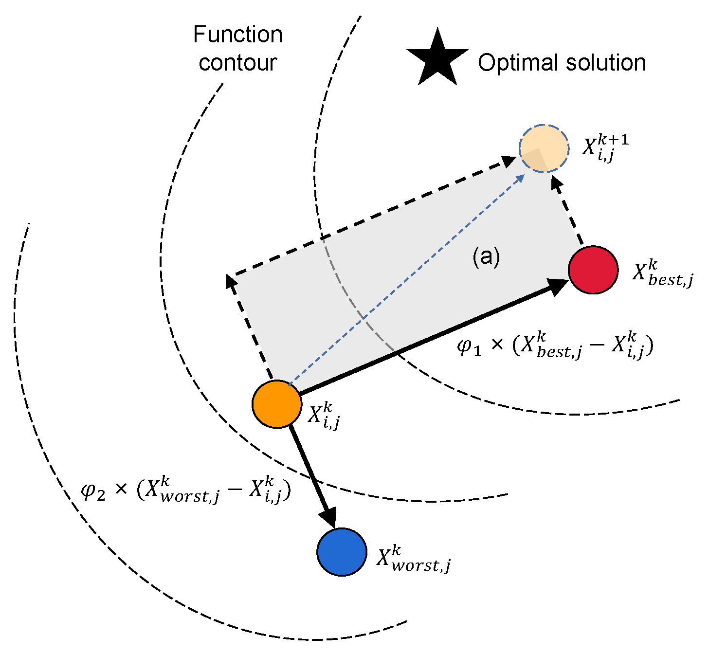
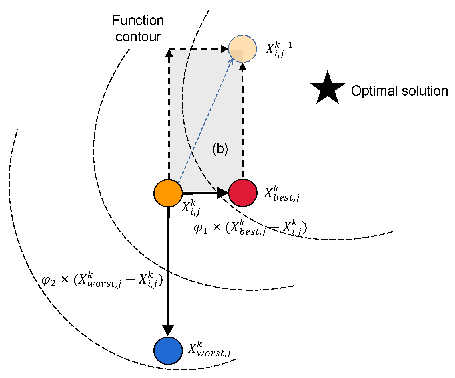
where ϕ 1 , ϕ 2 [ 0 , 1 ] are uniformly distributed random variables. Due to the limited range of ϕ 1 and ϕ 2 , the particle step size is constrained, especially when a particle is close to the best or worst positions, potentially causing the updated position to fall within the shaded regions shown in Figure 2 and Figure 3. Specifically,
  • When a particle is near the worst point X worst , j k , since | X i , j k X worst , j k |   0 , the update step is mainly determined by ϕ 1 X best , j k | X i , j k | . If ϕ 1 is small, the particle cannot effectively move away from the worst point, limiting global exploration.
  • When a particle is near the best point X best , j k , since | X i , j k X best , j k |   0 , the update step is primarily governed by ϕ 2 X worst , j k | X i , j k | . If ϕ 2 is small, the particle struggles to escape the local optimum, and its updated position may remain confined within a local region.
Moreover, the absolute value operation further restricts the flexibility of the update direction, causing the particle positions to be constrained within a certain region and thus forming the shaded areas.
To overcome this limitation, the Lévy flight mechanism is incorporated into Strategy 1. By introducing random perturbations drawn from a Lévy distribution into the update step, particles gain enhanced jump capability, allowing them to escape local optima while still performing small-scale local searches. Theoretically, the heavy-tailed property of Lévy flights enables particles to balance global exploration and local exploitation, thereby improving the overall algorithm performance. The updated formula is expressed as
X i , j k + 1 = X i , j k + L ( γ ) ϕ 1 X best , j k | X i , j k | ϕ 2 X worst , j k | X i , j k | ,
where L ( γ ) represents a random number drawn from a Lévy distribution. It should be noted that, compared to the original CLJAYA algorithm, the only additional parameter required in the equation is the power law exponent γ . Although this change is relatively simple, the new distribution significantly enhances the overall performance of the solution during optimization. Particle update strategies 2 and 3 inherit the update strategy of the original CLJAYA algorithm, fully utilizing population information to update particle positions based on the average position M of population particles [39].
X i , j a + 1 = X i , j a + L ( γ ) ϕ 1 ( X b e s t , j a | X i , j a | ) ϕ 2 ( X w o r s t , j a | X i , j a | ) , if 0 P s w i t c h 1 3 ,
X i , j a + 1 = X i , j a + ϕ 3 ( X b e s t , j a     | X i , j a | ) ϕ 4 ( M     | X i , j a | ) , if 1 3 < P s w i t c h 2 3 ,
X i , j a + 1 = X i , j a + ϕ 5 ( X b e s t , j a     | X i , j a | ) ϕ 6 ( X p , j a     | X q , j a | ) , if 2 3 < P s w i t c h 1 .
The CLJAYA-LF algorithm, summarized in Algorithm 1, proceeds by initializing the population, computing the fitness values, and then iteratively updating solutions using multiple strategies based on randomly selected individuals. After each update, the fitness is evaluated, and the population is revised if improvements are found. The process continues until convergence, and the best solution is returned. In the CLJAYA-LF algorithm, several key parameters and variables are used to control the optimization process. The population size N determines the number of particles, while I t m a x sets the maximum number of iterations, controlling when the algorithm terminates. The problem dimension d i m specifies the number of decision variables for each particle, and l b and u b define the lower and upper bounds for each variable, thereby constraining the search space.
Algorithm 1 The CLJAYA-LF Algorithm
Require: 
N, I t m a x , d i m , l b , u b
Ensure: 
B e s t V a l u e , X T a r g e t , B e s t C o s t
  1:
 Randomly initialize the population X within the bounds [ l b , u b ] with dimension d i m .
  2:
 Compute the fitness values f ( · ) for each individual in the population.
  3:
 Main Loop
  4:
 for  i = 1 to I t m a x  do
  5:
  Find the best solution B e s t and the worst solution W o r s t .
  6:
  Initialize a new solution matrix x new .
  7:
  for  j = 1 to n P o p  do
  8:
        Randomly select two individuals a and b different from the current individual j.
  9:
        Generate a random number P s w i t c h uniformly in [ 0 , 1 ] .
10:
        if  P s w i t c h 1 3  then
11:
            Update x new ( j , : ) using the first strategy (9a).
12:
        else if  P switch 2 3  then
13:
            Update x new ( j , : ) using the second strategy (9b).
14:
        else
15:
            Update x new ( j , : ) using the third strategy (9c).
16:
        end if
17:
        Ensure x new ( j , : ) is within the bounds [ l b , u b ] .
18:
        Compute the fitness f new ( j ) for the new solution.
19:
  end for
20:
  Replace the current population with the new solutions if the fitness improves.
21:
  Update the best solution B e s t and track the best fitness value.
22:
 end for
Require: 
Return the best fitness value B e s t V a l u e , the best solution X T a r g e t and the convergence curve B e s t C o s t
During the iterative update process, x new stores the updated particle positions after applying the selected strategy. In Strategy 3, X p , j and X q , j are randomly selected particle positions that introduce diversity into the population. The uniform random numbers ϕ 3 , ϕ 4 , ϕ 5 , and ϕ 6 control the step size and direction in Strategies 2 and 3, while P s w i t c h is a random variable used to determine which strategy is applied for each particle. After each update, the fitness value of the new particle is computed as f new , and B e s t C o s t records the best fitness value found in each iteration for monitoring convergence.

4. Applications of CLJAYA-LF on Numerical Optimization

To rigorously and convincingly demonstrate the superior performance of the CLJAYA-LF algorithm, this section presents a comprehensive performance evaluation using the CEC2017 benchmark suite [40]. The CEC2017 test set comprises optimization problems derived from real-world scenarios, mathematical models, and artificially constructed benchmark challenges, offering significant complexity and diversity to address a wide range of optimization problems. It consists of 29 functions, categorized into four types: unimodal functions (F1 and F3), which assess algorithm performance in simple scenarios with a single global optimum; multimodal functions (F4–F10), which evaluate the algorithm’s ability to escape local optima and identify the global optimum; composite functions (F11–F20), which combine basic functions to simulate real-world problems with multiple interacting factors; and hybrid functions (F21–F30), which model complex engineering scenarios incorporating continuous and discrete variables or various operational rules. These diverse function types collectively enable a comprehensive evaluation of the algorithm’s performance under varied conditions, making the CEC2017 benchmark particularly well suited for assessing the effectiveness of the CLJAYA-LF algorithm.
Notably, to ensure the fairness and credibility of the performance evaluation, all parameter settings in this study adhere strictly to the standards specified in the relevant references. Specifically, the parameter configurations of all comparative algorithms follow the settings documented in the corresponding reference literature to maintain consistency with the original validation conditions. Meanwhile, the test parameters for the CEC2017 benchmark suite and the experimental parameters for various engineering problems are all directly adopted from the verified and mature configurations in the relevant references, without any arbitrary adjustments. This practice not only guarantees a high degree of consistency between the experimental conditions of this study and the literature benchmarks, eliminating interference from parameter deviations on the evaluation results, but also establishes a unified and comparable experimental framework for the performance comparison between the CLJAYA-LF algorithm and other comparative algorithms, laying a solid foundation for the objectivity and rigor of the subsequent evaluation conclusions.
Performance Comparison of Multiple Algorithms on CEC2017 Test Suite
To clearly demonstrate the advantages and disadvantages of the proposed method compared to other well-established algorithms of the same kind, we specifically selected several widely used and highly reputed algorithms in the field of optimization for performance comparison, including the PSO algorithm [13], HHO algorithm [18], DMO algorithm [19], SABO algorithm [29], JAYA algorithm [30], JAYA-LF algorithm [32], and CLJAYA algorithm [33]. To ensure a fair comparison of the 50-dimensional optimization problems of CEC2017, the population size and the maximum number of function evaluations for all algorithms were set to 100 and 1000, respectively. Each algorithm was independently run 100 times on each test function, and the mean absolute error (Mean) and standard deviation (STD) were recorded for each test function.
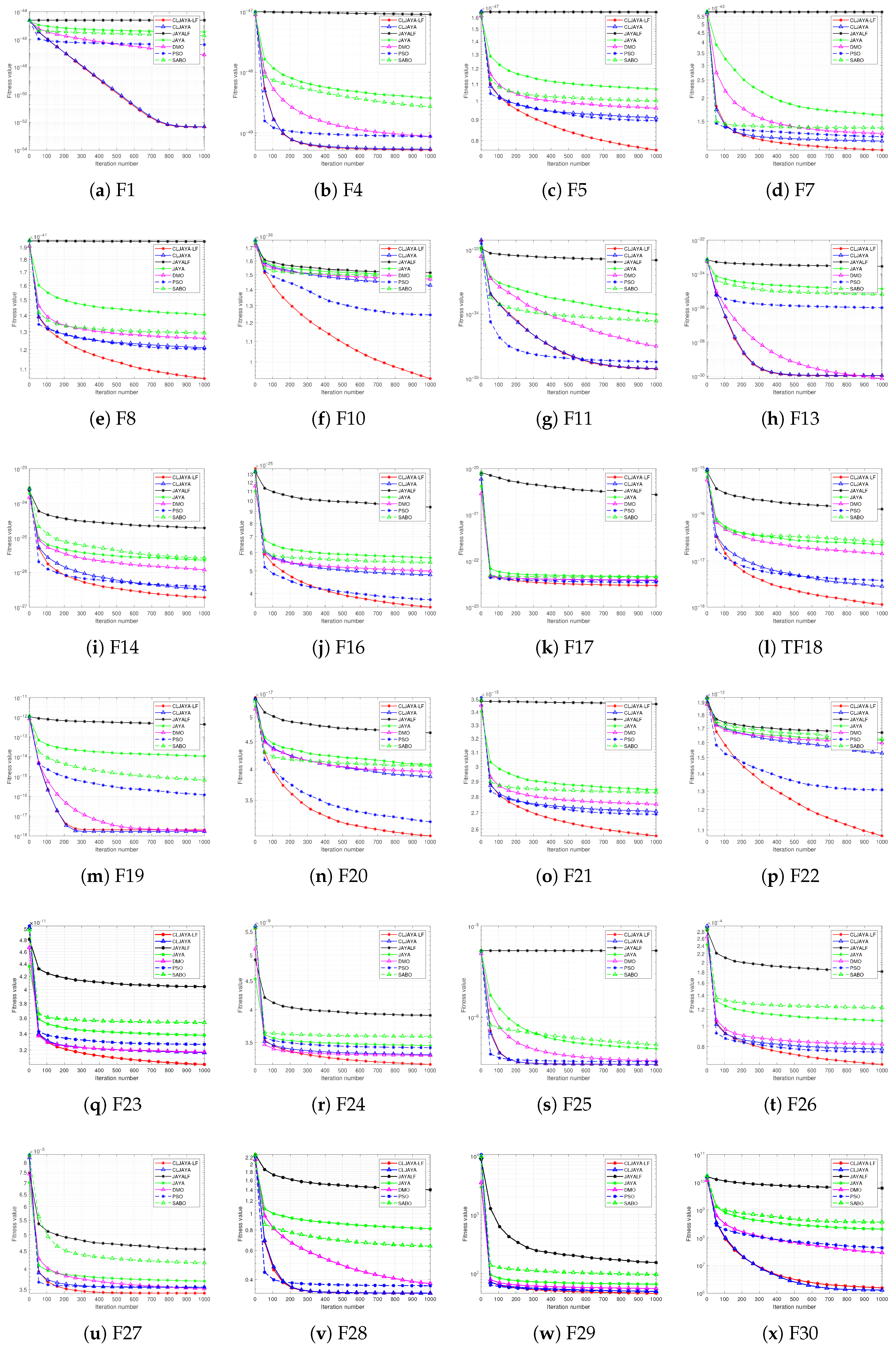
In Figure 4, it can be seen that in the optimization of unimodal functions (F1, F3), the CLJAYA-LF proposed in this paper exhibits smaller fitness value updates compared to the existing JAYA, JAYALF, and CLJAYA in F1, demonstrating optimal performance. In the optimization of simple multimodal functions (F4–F10), CLJAYA-LF demonstrates significantly better performance than JAYA, JAYALF, and CLJAYA in F4, F5, F7, F8, and F10. In the optimization of hybrid function (F11–F20), CLJAYA-LF shows significantly better performance than JAYA, JAYALF, CLJAYA, and other algorithms in F11, F14, F16–F18, and F20. In the optimization of composition functions (F21–F30), CLJAYA-LF significantly outperforms JAYA, JAYALF, CLJAYA, and other algorithms on F21–F29. Its performance is slightly inferior to CLJAYA in F30. Therefore, CLJAYA-LF demonstrates robust and superior optimization capabilities, making it a highly effective algorithm to solve complex optimization problems.
From the analysis of Table 1, the following conclusions can be drawn regarding the variance performance of the CLJAYA-LF algorithm on 22 functions with better performance. It is observed that in 15 of these 22 functions, CLJAYA-LF exhibits variance comparable to that of other methods, indicating that the algorithm not only achieves superior optimization performance but also maintains similar stability to existing methods, with relatively balanced variance control.
We conducted a comparative performance analysis of the proposed CLJAYA algorithm on the 100-dimensional optimization problems from CEC2017. For both CLJAYA and the other algorithms, the population size was set to 150, and the maximum number of function evaluations was set to 1000. Each algorithm was independently executed 100 times on each test function. The relevant results are presented in Figure 5 and Table 2.
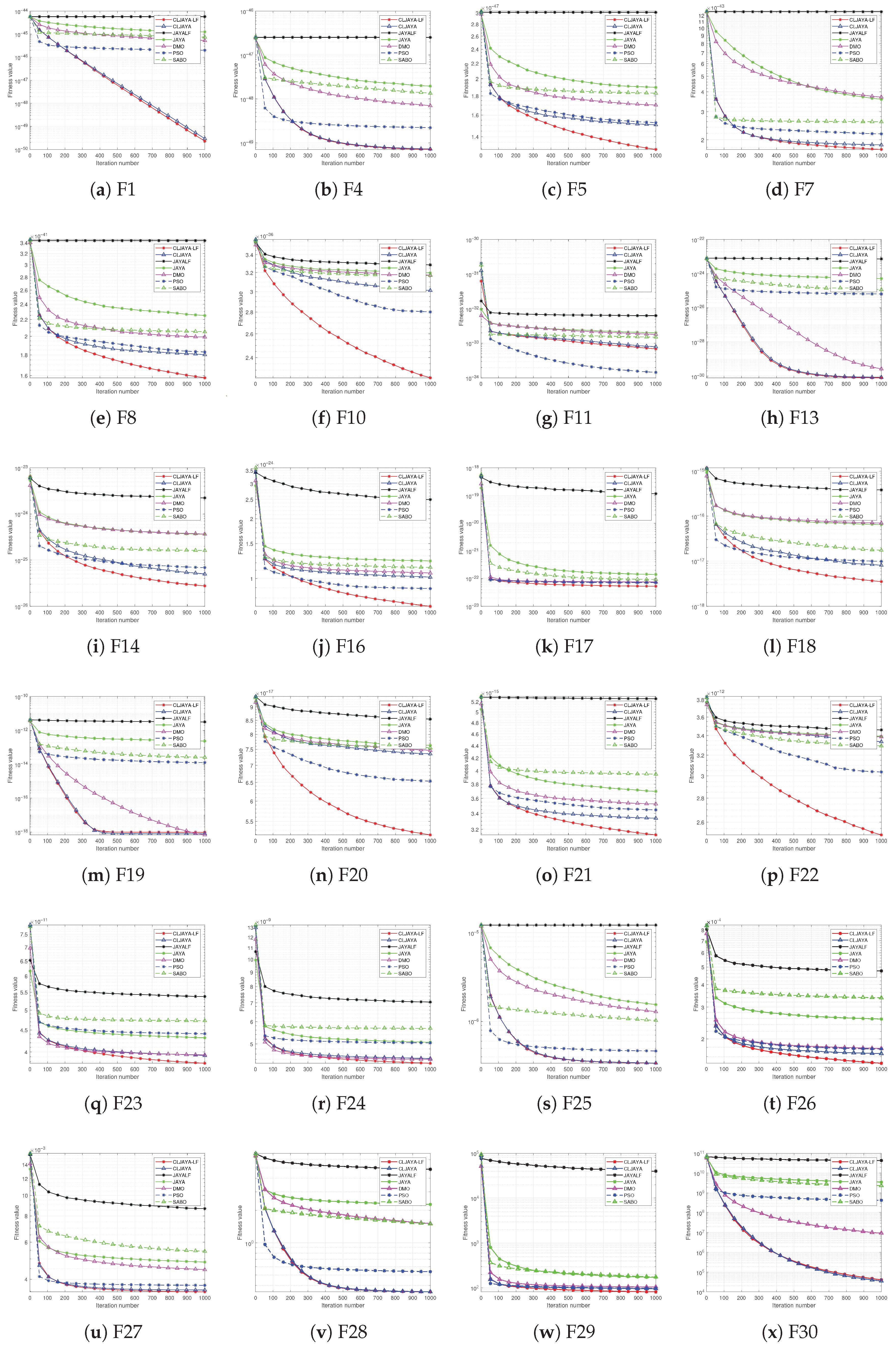
In Figure 5, it can be observed that the proposed CLJAYA-LF algorithm demonstrates smaller fitness value updates compared to existing algorithms, achieving optimal performance in F1, F4, F5, F7, F8, F10, F13, F14, F16, F17, F18, F20, and F21–F29. Although its performance is slightly inferior to CLJAYA on F30, there is a significant improvement in performance at 100 dimensions compared to the results at 50 dimensions.
From the analysis of Table 2, the following conclusions can be drawn: The CLJAYA-LF algorithm demonstrates smaller variance across 24 functions, with its variance outperforming the existing methods in 17 of these functions. This indicates that the algorithm not only achieves superior optimization performance but also maintains similar stability to the existing methods, with relatively balanced variance control. Compared to the 50-dimensional problems, the proposed algorithm shows better performance in the 100-dimensional case, proving that the method is not only suitable for high-dimensional optimization problems but also outperforms existing algorithms in such high-dimensional problems.

5. Applications of CLJAYA on Engineering Optimization

5.1. Step-Cone Pulley Problem

The main objective of this optimization problem is to minimize the weight of a four-step cone pulley by adjusting five design variables [41]. These variables include the diameters of the four steps of the pulley and the width of the pulley. During the optimization process, 11 non-linear constraints must be met to ensure that the pulley design meets practical performance requirements. One key constraint is that the output power of the pulley system must be at least 0.75 horsepower (hp). These nonlinear constraints involve limitations on the pulley’s dimensions, material strength requirements, transmission ratio conditions, compatibility with other components, and overall system efficiency. These constraints ensure that the designed pulley is not only lightweight but also has excellent mechanical performance and durability, meeting the demands of real-world engineering applications.
The experimental results are shown in Table 3. It is found that the mean value of the algorithm proposed in this paper is 1.69 × 101, and the variance is 3.32 × 10⁻¹. These values are significantly smaller than the corresponding values of all other comparative algorithms, which fully demonstrates that the algorithm proposed in this paper has better stability and reliability, indicating that the proposed algorithm has a stronger global search ability. The worst value can reflect the algorithm’s risk-resistant ability under adverse conditions, and the median reflects the algorithm’s anti-interference performance, that is, the adaptability of the algorithm. The worst value of the algorithm proposed in this paper is 1.78 × 101, which is slightly lower than that of the CLJAYA algorithm. The median is 1.69 × 101, which is equal to the median of the CLJAYA algorithm, but both are significantly lower than those of the remaining algorithms. This indicates that the algorithm proposed in this paper is superior to existing algorithms in terms of adaptability. The best value can be used to measure the potential of the algorithm. The best value of the algorithm proposed in this paper is slightly higher than that of the CLJAYA and DMO algorithms. However, the DMO algorithm has poor stability, as its STD is high. Therefore, the algorithm proposed in this paper has a good potential similar to that of the CLJAYA algorithm.

5.2. Gear Train Design Problem

The gear system design problem is a classic example in the field of structural optimization. The objective is to determine the optimal number of teeth for each gear through proper parameter design, achieving performance optimization while meeting the design requirements. This problem involves four integer decision variables, each representing the number of teeth in a gear. The mathematical formulation of this problem is presented in [42].
As shown in Table 4, it is found that the mean of the algorithm proposed in this paper is 1.44 × 10⁻¹⁵, and the STD is 3.14 × 10⁻¹⁵. Compared with algorithms such as JAYA, JAYALF, CLJAYA, DMO, SABO, and PSO, the mean and variance of the algorithm proposed in this paper are significantly smaller. However, there is still a certain gap compared to the HHO algorithm. This fully demonstrates that, compared to the existing JAYA and its series of improved algorithms, the algorithm proposed in this paper performs outstandingly in terms of stability, reliability, and global search ability. However, in terms of overall performance, it is temporarily inferior to the HHO algorithm.
Among the evaluation indicators of algorithm performance, the worst value can directly reflect the algorithm’s ability to resist risks under adverse conditions, while the median mainly reflects the algorithm’s anti-interference performance, which is directly related to the algorithm’s adaptability. The worst value of the algorithm proposed in this paper is 1.93 × 10⁻¹⁴, and the median is 2.14 × 10⁻¹⁶. In horizontal comparison with algorithms such as JAYA, JAYALF, CLJAYA, DMO, SABO, and PSO, these two key indicators are significantly lower. However, compared to the HHO algorithm, there is still room for improvement. This clearly indicates that in terms of adaptability, the algorithm proposed in this paper has obvious advantages among the existing algorithms, being only slightly inferior to the HHO algorithm.
The best value serves as a crucial criterion for assessing an algorithm’s potential. Through comparison, it is evident that the optimal value of the algorithm presented in this paper is marginally lower than that of the CLJAYA, PSO, and HHO algorithms. Given this outcome, the exploration of the potential of the proposed algorithm must be conducted more thoroughly. This involves further strengthening its capacity to seek the optimal solution, thereby achieving a comprehensive enhancement of the algorithm’s performance.

5.3. Planetary Gear Train Design Problem

This problem aims to minimize the maximum error in the gear transmission ratio through optimization design. To achieve this, the total number of teeth for each gear in the automatic planetary transmission system must first be determined. The maximum transmission ratio error refers to the deviation between the actual and ideal transmission ratios. By minimizing this error, the transmission efficiency of the system can be improved, ensuring smooth vehicle operation under different working conditions [43].
As shown in Table 5, the CLJAYA-LF algorithm has several remarkable characteristics. First of all, it exhibits excellent performance and features high stability and reliability. Its best value is 5.26 × 10⁻¹, which indicates that it has a similar performance to algorithms such as CLJAYA and JAYA in terms of finding the optimal solution. Compared to CLJAYA and JAYA, the relatively low standard deviation of 4.98 × 10⁻² means that it has lower variability and higher consistency during multiple runs, suggesting that it is more effective in handling random factors. The mean value of 5.35 × 10⁻¹ is lower than that of CLJAYA, showing strong overall performance. In addition, the worst-case value of 8.90 × 10⁻¹ indicates that it outperforms JAYALF and JAYA, highlighting its good robustness under adverse conditions. In conclusion, the CLJAYA-LF has strong performance and is suitable for applications that require stability and reliability. CLJAYA-LF demonstrates excellent optimization performance. Its best value (1.62 × 101) is slightly worse than CLJAYA’s best value (1.61 × 101). The standard deviation (3.32 × 101) suggests that CLJAYA-LF exhibits small fluctuations in multiple runs, offering high stability. These two indicators indicate comparable optimization capabilities. The mean value (1.69 × 101), which is close to the best value, confirms its stable and reliable optimization results. The median value (1.70 × 101) shows that most of the results are close to the optimal solution. Even in the worst case (1.78 × 101), CLJAYA-LF still maintains a high solution quality compared to other methods, making it a stable and efficient optimization algorithm suitable for complex problems.

6. Conclusions

In this study, the CLJAYA-LF algorithm was proposed, and its performance was rigorously verified through numerous experiments. By incorporating the Lévy Flight method, the CLJAYA-LF algorithm enhances its global search capabilities while maintaining favorable local search performance, effectively resolving the issue of traditional algorithms being prone to being trapped in local optima. The experimental results indicate that the CLJAYA-LF algorithm demonstrates outstanding performance in terms of stability, efficiency, and global optimization ability. It can achieve excellent results in various engineering problems, especially showing significant advantages when dealing with complex non-linear problems. The low standard deviation obtained from multiple runs reflects its high stability, and the characteristic of rapidly converging to better solutions makes it suitable for scenarios with high requirements for real-time performance and efficiency. In conclusion, the CLJAYA-LF algorithm breaks through traditional limitations, improving optimization accuracy and efficiency, thus possessing both theoretical value and broad application prospects.
Although the performance of CLJAYA has improved compared to the existing JAYA and its improved algorithms, there is still a gap in the local mining ability compared to algorithms such as HHO. In the future, we plan to introduce advanced techniques like reinforcement learning to dynamically adjust the update strategy, aiming to improve the local mining ability of the algorithm and further enhance its performance.

Author Contributions

Writing—original draft preparation, X.S.; writing—review and editing, X.L. All authors have read and agreed to the published version of the manuscript.

Funding

This work was supported by the Guangxi Science and Technology Major Program under Grant Nos. 2024AA19022 and 2024AA29091.

Institutional Review Board Statement

Not applicable.

Informed Consent Statement

Not applicable.

Data Availability Statement

Data are contained within the article.

Conflicts of Interest

The authors declare no conflicts of interest.

References

  1. Diwekar, U.M. Introduction to Applied Optimization; Springer Nature: Berlin/Heidelberg, Germany, 2020; Volume 22. [Google Scholar]
  2. Dantzig, G.B. Linear Programming and Extensions; Princeton University Press: Princeton, NJ, USA, 1963. [Google Scholar] [CrossRef]
  3. Pérez, L.V.; Bossio, G.R.; Moitre, D.; García, G.O. Optimization of power management in an hybrid electric vehicle using dynamic programming. Math. Comput. Simul. 2006, 73, 244–254. [Google Scholar] [CrossRef]
  4. Sebastian, R. An overview of gradient descent optimization algorithms. arXiv 2016, arXiv:1609.04747. [Google Scholar]
  5. Korani, W.; Mouhoub, M. Review on nature-inspired algorithms. SN Oper. Res. Forum 2021, 2, 36. [Google Scholar] [CrossRef]
  6. Katoch, S.; Chauhan, S.S.; Kumar, V. A review on genetic algorithm: Past, present, and future. Multimed. Tools Appl. 2021, 80, 8091–8126. [Google Scholar] [CrossRef] [PubMed]
  7. Hansen, N.; Arnold, D.V.; Auger, A. Evolution strategies. In Handbook of Computational Intelligence; Springer: Berlin/Heidelberg, Germany, 2015; pp. 871–898. [Google Scholar]
  8. Price, K.V. Differential evolution. In Handbook of Optimization: From Classical to Modern Approach; Springer: Berlin/Heidelberg, Germany, 2013; pp. 187–214. [Google Scholar]
  9. Chen, H.; Li, X.; Li, S.; Zhao, Y.; Dong, J. Improved Slime Mould Algorithm Hybridizing Chaotic Maps and Differential Evolution Strategy for Global Optimization. IEEE Access 2022, 10, 66811–66830. [Google Scholar] [CrossRef]
  10. Gao, H.; Zhang, Q. Alpha evolution: An efficient evolutionary algorithm with evolution path adaptation and matrix generation. Eng. Appl. Artif. Intell. 2024, 137, 109202. [Google Scholar] [CrossRef]
  11. Stergiou, K.; Karakasidis, T. Optimizing Renewable Energy Systems Placement Through Advanced Deep Learning and Evolutionary Algorithms. Appl. Sci. 2024, 14, 10795. [Google Scholar] [CrossRef]
  12. Jiang, X.; Li, S. BAS: Beetle Antennae Search Algorithm for Optimization Problems. arXiv 2017, arXiv:1710.10724. [Google Scholar] [CrossRef]
  13. Eberhart, R.; Kennedy, J. Particle swarm optimization. In Proceedings of the IEEE International Conference on NEURAL Networks, Perth, WA, Australia, 27 November–1 December 1995; Citeseer: Princeton, NJ, USA, 1995; Volume 4, pp. 1942–1948. [Google Scholar]
  14. Yue, F.; Sha, Z.; Sun, H.; Chen, D.; Liu, J. Research on the Optimization of TP2 Copper Tube Drawing Process Parameters Based on Particle Swarm Algorithm and Radial Basis Neural Network. Appl. Sci. 2024, 14, 11203. [Google Scholar] [CrossRef]
  15. Kumar De, S.; Banerjee, A.; Majumder, K.; Kotecha, K.; Abraham, A. Coverage Area Maximization Using MOFAC-GA-PSO Hybrid Algorithm in Energy Efficient WSN Design. IEEE Access 2023, 11, 99901–99917. [Google Scholar] [CrossRef]
  16. Karaboga, D.; Gorkemli, B.; Ozturk, C.; Karaboga, N. A comprehensive survey: Artificial bee colony (ABC) algorithm and applications. Artif. Intell. Rev. 2014, 42, 21–57. [Google Scholar] [CrossRef]
  17. Faris, H.; Aljarah, I.; Al-Betar, M.A.; Mirjalili, S. Grey wolf optimizer: A review of recent variants and applications. Neural Comput. Appl. 2018, 30, 413–435. [Google Scholar] [CrossRef]
  18. Alabool, H.M.; Alarabiat, D.; Abualigah, L.; Heidari, A.A. Harris hawks optimization: A comprehensive review of recent variants and applications. Neural Comput. Appl. 2021, 33, 8939–8980. [Google Scholar] [CrossRef]
  19. Agushaka, J.O.; Ezugwu, A.E.; Abualigah, L. Dwarf mongoose optimization algorithm. Comput. Methods Appl. Mech. Eng. 2022, 391, 114570. [Google Scholar] [CrossRef]
  20. Chen, Z.; Francis, A.; Li, S.; Liao, B.; Xiao, D.; Ha, T.T.; Li, J.; Ding, L.; Cao, X. Egret Swarm Optimization Algorithm: An Evolutionary Computation Approach for Model Free Optimization. Biomimetics 2022, 7, 144. [Google Scholar] [CrossRef]
  21. Lian, J.; Hui, G. Human evolutionary optimization algorithm. Expert Syst. Appl. 2024, 241, 122638. [Google Scholar] [CrossRef]
  22. Zhou, G.; Zhou, Y.; Deng, W.; Yin, S.; Zhang, Y. Advances in teaching–learning-based optimization algorithm: A comprehensive survey(ICIC2022). Neurocomputing 2023, 561, 126898. [Google Scholar] [CrossRef]
  23. Al-Masri, O.; Al-Sorori, W.A. Object-Oriented Test Case Generation Using Teaching Learning-Based Optimization (TLBO) Algorithm. IEEE Access 2022, 10, 110879–110888. [Google Scholar] [CrossRef]
  24. Oladejo, S.O.; Ekwe, S.O.; Mirjalili, S. The Hiking Optimization Algorithm: A novel human-based metaheuristic approach. Knowl.-Based Syst. 2024, 296, 111880. [Google Scholar] [CrossRef]
  25. Chen, Z.; Li, S.; Khan, A.T.; Mirjalili, S. Competition of tribes and cooperation of members algorithm: An evolutionary computation approach for model free optimization. Expert Syst. Appl. 2025, 265, 125908. [Google Scholar] [CrossRef]
  26. Rutenbar, R.A. Simulated annealing algorithms: An overview. IEEE Circuits Devices Mag. 1989, 5, 19–26. [Google Scholar] [CrossRef]
  27. Luo, K. Water flow optimizer: A nature-inspired evolutionary algorithm for global optimization. IEEE Trans. Cybern. 2021, 52, 7753–7764. [Google Scholar] [CrossRef]
  28. Hashim, F.A.; Mostafa, R.R.; Hussien, A.G.; Mirjalili, S.; Sallam, K.M. Fick’s Law Algorithm: A physical law-based algorithm for numerical optimization. Knowl.-Based Syst. 2023, 260, 110146. [Google Scholar] [CrossRef]
  29. Trojovskỳ, P.; Dehghani, M. Subtraction-average-based optimizer: A new swarm-inspired metaheuristic algorithm for solving optimization problems. Biomimetics 2023, 8, 149. [Google Scholar] [CrossRef]
  30. Rao, R. Jaya: A simple and new optimization algorithm for solving constrained and unconstrained optimization problems. Int. J. Ind. Eng. Comput. 2016, 7, 19–34. [Google Scholar] [CrossRef]
  31. Teng, Z.; Li, M.; Yu, L.; Gu, J.; Li, M. Sinkhole Attack Defense Strategy Integrating SPA and Jaya Algorithms in Wireless Sensor Networks. Sensors 2023, 23, 9709. [Google Scholar] [CrossRef]
  32. Iacca, G.; dos Santos Junior, V.C.; de Melo, V.V. An improved Jaya optimization algorithm with Lévy flight. Expert Syst. Appl. 2021, 165, 113902. [Google Scholar] [CrossRef]
  33. Zhang, Y.; Jin, Z. Comprehensive learning Jaya algorithm for engineering design optimization problems. J. Intell. Manuf. 2022, 33, 1229–1253. [Google Scholar] [CrossRef]
  34. Viswanathan, G.M.; Buldyrev, S.V.; Havlin, S.; da Luz, M.G.; Raposo, E.P.; Stanley, H.E. Optimizing the success of random searches. Nature 1999, 401, 911–914. [Google Scholar] [CrossRef] [PubMed]
  35. Wu, L.; Wu, J.; Wang, T. Enhancing grasshopper optimization algorithm (GOA) with levy flight for engineering applications. Sci. Rep. 2023, 13, 124. [Google Scholar] [CrossRef]
  36. Heidari, A.A.; Pahlavani, P. An efficient modified grey wolf optimizer with Lévy flight for optimization tasks. Appl. Soft Comput. 2017, 60, 115–134. [Google Scholar] [CrossRef]
  37. He, Q.; Liu, H.; Ding, G.; Tu, L. A modified Lévy flight distribution for solving high-dimensional numerical optimization problems. Math. Comput. Simul. 2023, 204, 376–400. [Google Scholar] [CrossRef]
  38. Mohiz, M.J.; Baloch, N.K.; Hussain, F.; Saleem, S.; Zikria, Y.B.; Yu, H. Application mapping using cuckoo search optimization with Lévy flight for NoC-based system. IEEE Access 2021, 9, 141778–141789. [Google Scholar] [CrossRef]
  39. Shen, X.; Sunat, K. A Novel Comprehensive Learning JAYA Algorithm Based on Lévy Flights. In Proceedings of the 2024 28th International Computer Science and Engineering Conference (ICSEC), Khon Kaen, Thailand, 6–8 November 2024; IEEE: New York, NY, USA, 2024; pp. 1–5. [Google Scholar]
  40. Wu, G.; Mallipeddi, R.; Suganthan, P. Problem Definitions and Evaluation Criteria for the CEC 2017 Competition and Special Session on Constrained Single Objective Real-Parameter Optimization; Nanyang Technological University: Singapore, 2016. [Google Scholar]
  41. Yusof, N.J.; Kamaruddin, S. Optimal design of step–cone pulley problem using the bees algorithm. In Intelligent Manufacturing and Mechatronics: Proceedings of SympoSIMM 2020; Springer: Berlin/Heidelberg, Germany, 2021; pp. 139–149. [Google Scholar]
  42. Jangir, P.; Buch, H.; Mirjalili, S.; Manoharan, P. MOMPA: Multi-objective marine predator algorithm for solving multi-objective optimization problems. Evol. Intell. 2023, 16, 169–195. [Google Scholar] [CrossRef]
  43. Daoudi, K.; Boudi, E.M. Optimal volume design of planetary gear train using particle swarm optimization. In Proceedings of the 2018 4th International Conference on Optimization and Applications (ICOA), Mohammedia, Morocco, 26–27 April; IEEE: New York, NY, USA, 2018; pp. 1–4. [Google Scholar]
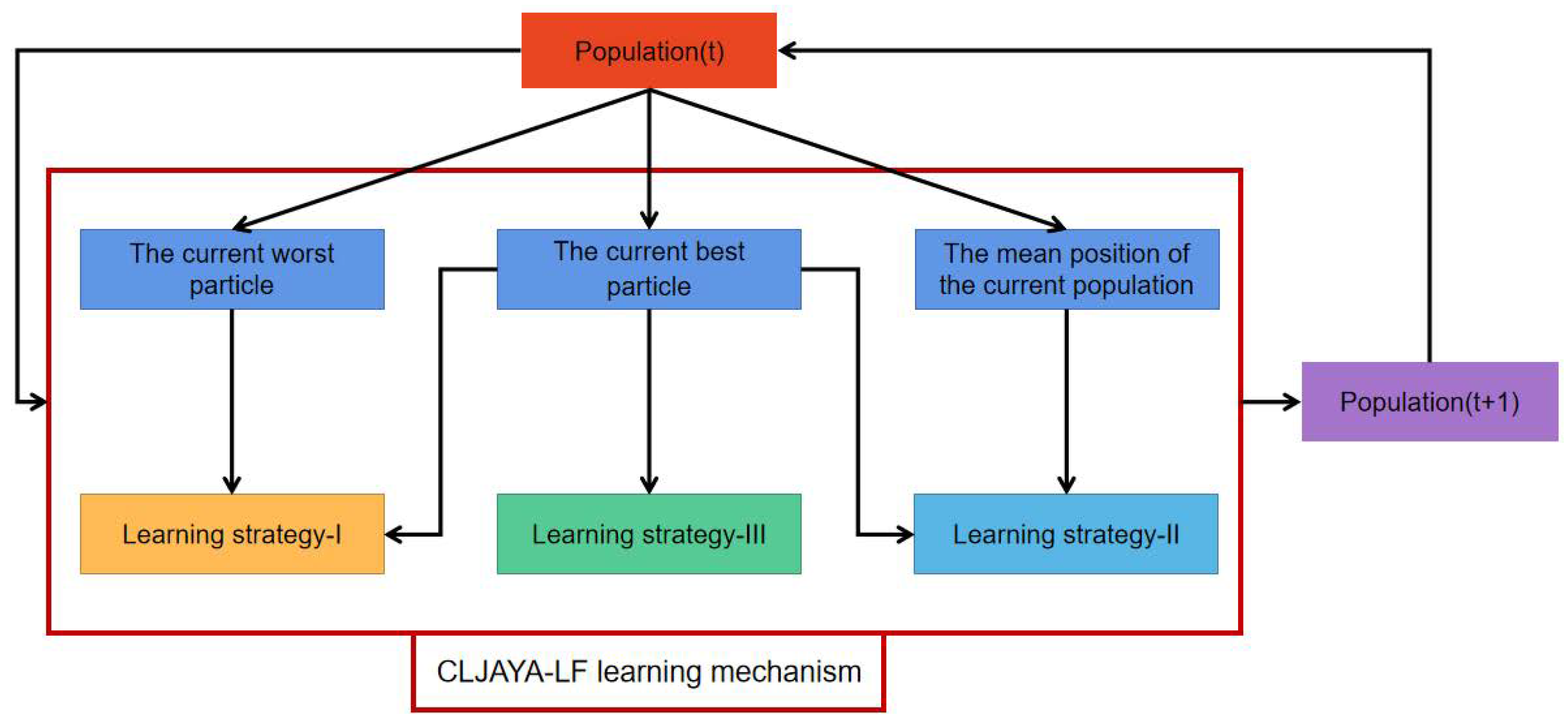
Figure 1. CLJAYA-LF framework diagram.
Electronics 14 03776 g001
Figure 2. Particle update strategy 1 near worst particle.
Electronics 14 03776 g002
Figure 3. Particle update strategy 1 near best particle.
Electronics 14 03776 g003
Figure 4. Several convergence curves obtained using CLJAYA-LF, JAYA, CLJAYA, and other algorithms on 50-dimensional problems of the CEC2017 test suite. Panels are labeled as (a) F1, (b) F4, (c) F5, (d) F7, (e) F8, (f) F10, (g) F11, (h) F13, (i) F14, (j) F16, (k) F17, (l) TF18, (m) F19, (n) F20, (o) F21, (p) F22, (q) F23, (r) F24, (s) F25, (t) F26, (u) F27, (v) F28, (w) F29, (x) F30.
Electronics 14 03776 g004
Figure 5. Several convergence curves obtained using CLJAYA-LF, JAYA, CLJAYA, and other algorithms on 100-dimensional problems of the CEC2017 test suite. Panels are labeled as (a) F1, (b) F4, (c) F5, (d) F7, (e) F8, (f) F10, (g) F11, (h) F13, (i) F14, (j) F16, (k) F17, (l) F18, (m) F19, (n) F20, (o) F21, (p) F22, (q) F23, (r) F24, (s) F25, (t) F26, (u) F27, (v) F28, (w) F29, (x) F30.
Electronics 14 03776 g005
Table 1. CEC2017 50D: algorithmic performance comparison.
No. Ind. CLJAYA-LF CLJAYA JAYALF JAYA DMO HHO SABO PSO
F1STD 5.87 × 10 3 6.01 × 10 3 2.24 × 10 10 4.27 × 10 9 1.31 × 10 8 1.28 × 10 7 5.53 × 10 9 2.40 × 10 9
F1Mean 4.49 × 10 3 5.07 × 10 3 2.40 × 10 11 3.49 × 10 10 7.57 × 10 8 7.30 × 10 7 1.73 × 10 10 3.97 × 10 9
F3STD 2.63 × 10 4 2.30 × 10 4 7.46 × 10 4 4.17 × 10 4 2.88 × 10 4 1.17 × 10 4 1.35 × 10 4 1.68 × 10 4
F3Mean 1.66 × 10 5 1.73 × 10 5 5.47 × 10 5 2.74 × 10 5 2.67 × 10 5 5.29 × 10 4 1.61 × 10 5 7.31 × 10 4
F4STD 4.73 × 10 1 4.84 × 10 1 1.19 × 10 4 7.72 × 10 2 3.76 × 10 1 6.80 × 10 1 1.05 × 10 3 2.21 × 10 2
F4Mean 5.24 × 10 2 5.30 × 10 2 8.81 × 10 4 3.62 × 10 3 8.72 × 10 2 6.75 × 10 2 2.81 × 10 3 8.96 × 10 2
F5STD 2.39 × 10 1 1.89 × 10 1 6.50 × 10 1 3.08 × 10 1 1.70 × 10 1 2.96 × 10 1 4.41 × 10 1 4.39 × 10 1
F5Mean 7.55 × 10 2 9.12 × 10 2 1.65 × 10 3 1.07 × 10 3 9.60 × 10 2 8.83 × 10 2 1.01 × 10 3 8.95 × 10 2
F6STD 2.91 × 10 0 2.06 × 10 1 7.58 × 10 0 5.62 × 10 0 1.21 × 10 0 4.63 × 10 0 1.20 × 10 1 6.28 × 10 0
F6Mean 6.03 × 10 2 6.00 × 10 2 7.45 × 10 2 6.59 × 10 2 6.13 × 10 2 6.72 × 10 2 6.58 × 10 2 6.24 × 10 2
F7STD 2.96 × 10 1 1.90 × 10 1 3.36 × 10 2 6.09 × 10 1 2.34 × 10 1 8.75 × 10 1 5.72 × 10 1 5.06 × 10 1
F7Mean 1.05 × 10 3 1.17 × 10 3 5.82 × 10 3 1.62 × 10 3 1.28 × 10 3 1.81 × 10 3 1.38 × 10 3 1.24 × 10 3
F8STD 2.18 × 10 1 1.90 × 10 1 6.89 × 10 1 3.22 × 10 1 1.74 × 10 1 3.07 × 10 1 3.66 × 10 1 4.72 × 10 1
F8Mean 1.03 × 10 3 1.21 × 10 3 1.94 × 10 3 1.41 × 10 3 1.26 × 10 3 1.17 × 10 3 1.29 × 10 3 1.19 × 10 3
F9STD 1.58 × 10 3 1.27 × 10 2 1.00 × 10 4 5.09 × 10 3 9.32 × 10 2 2.84 × 10 3 4.64 × 10 3 4.42 × 10 3
F9Mean 3.02 × 10 3 9.93 × 10 2 9.29 × 10 4 2.20 × 10 4 6.23 × 10 3 2.20 × 10 4 1.42 × 10 4 5.40 × 10 3
F10STD 4.43 × 10 2 1.16 × 10 3 4.73 × 10 2 3.91 × 10 2 3.90 × 10 2 8.38 × 10 2 3.93 × 10 2 8.54 × 10 2
F10Mean 9.16 × 10 3 1.43 × 10 4 1.51 × 10 4 1.49 × 10 4 1.47 × 10 4 9.05 × 10 3 1.48 × 10 4 1.24 × 10 4
F11STD 5.16 × 10 1 6.15 × 10 1 1.17 × 10 4 2.26 × 10 3 3.67 × 10 2 8.34 × 10 1 1.68 × 10 3 1.29 × 10 2
F11Mean 1.41 × 10 3 1.44 × 10 3 6.79 × 10 4 1.03 × 10 4 3.20 × 10 3 1.49 × 10 3 8.19 × 10 3 1.81 × 10 3
F12STD 2.69 × 10 6 2.17 × 10 6 9.34 × 10 9 1.33 × 10 9 5.40 × 10 7 3.92 × 10 7 2.05 × 10 9 6.98 × 10 8
F12Mean 4.89 × 10 6 3.68 × 10 6 8.11 × 10 10 7.04 × 10 9 3.68 × 10 8 8.88 × 10 7 3.77 × 10 9 7.59 × 10 8
F13STD 9.82 × 10 3 8.92 × 10 3 4.91 × 10 9 3.66 × 10 8 7.37 × 10 3 8.13 × 10 5 3.85 × 10 8 2.89 × 10 8
F13Mean 1.11 × 10 4 1.10 × 10 4 2.97 × 10 10 1.36 × 10 9 8.86 × 10 3 2.37 × 10 6 7.36 × 10 8 1.31 × 10 8
F14STD 1.33 × 10 5 2.40 × 10 5 7.60 × 10 6 1.19 × 10 6 3.92 × 10 5 5.21 × 10 5 1.58 × 10 6 2.91 × 10 5
F14Mean 1.86 × 10 5 3.48 × 10 5 2.13 × 10 7 2.26 × 10 6 1.23 × 10 6 7.30 × 10 5 2.32 × 10 6 4.33 × 10 5
F15STD 8.03 × 10 3 8.35 × 10 3 1.58 × 10 9 1.16 × 10 8 4.06 × 10 3 1.57 × 10 5 8.53 × 10 7 1.19 × 10 6
F15Mean 1.09 × 10 4 1.04 × 10 4 6.00 × 10 9 4.13 × 10 8 1.11 × 10 4 4.11 × 10 5 6.42 × 10 7 1.37 × 10 6
F16STD 2.41 × 10 2 3.57 × 10 2 6.07 × 10 2 2.58 × 10 2 1.99 × 10 2 4.68 × 10 2 5.47 × 10 2 4.61 × 10 2
F16Mean 3.48 × 10 3 4.82 × 10 3 9.37 × 10 3 5.65 × 10 3 4.99 × 10 3 4.30 × 10 3 5.32 × 10 3 3.74 × 10 3
F17STD 2.10 × 10 2 2.30 × 10 2 1.67 × 10 5 2.42 × 10 2 1.60 × 10 2 3.67 × 10 2 4.36 × 10 2 2.96 × 10 2
F17Mean 2.90 × 10 3 3.82 × 10 3 2.59 × 10 5 4.49 × 10 3 3.84 × 10 3 3.74 × 10 3 4.43 × 10 3 3.45 × 10 3
F18STD 8.56 × 10 5 1.86 × 10 6 4.38 × 10 7 8.38 × 10 6 4.52 × 10 6 3.16 × 10 6 1.40 × 10 7 2.27 × 10 6
F18Mean 1.12 × 10 6 3.43 × 10 6 1.37 × 10 8 2.23 × 10 7 1.45 × 10 7 3.99 × 10 6 2.30 × 10 7 3.50 × 10 6
F19STD 1.15 × 10 4 1.22 × 10 4 1.03 × 10 9 6.68 × 10 7 5.25 × 10 3 6.88 × 10 5 5.21 × 10 6 1.33 × 10 6
F19Mean 1.81 × 10 4 1.71 × 10 4 4.48 × 10 9 1.02 × 10 8 1.87 × 10 4 8.48 × 10 5 6.54 × 10 6 1.27 × 10 6
F20STD 1.64 × 10 2 2.00 × 10 2 1.52 × 10 2 1.69 × 10 2 1.53 × 10 2 3.04 × 10 2 1.80 × 10 2 2.94 × 10 2
F20Mean 3.00 × 10 3 3.88 × 10 3 4.67 × 10 3 4.07 × 10 3 3.95 × 10 3 3.35 × 10 3 4.05 × 10 3 3.17 × 10 3
F21STD 2.03 × 10 1 2.09 × 10 1 6.40 × 10 1 2.52 × 10 1 1.62 × 10 1 7.77 × 10 1 3.70 × 10 1 4.35 × 10 1
F21Mean 2.56 × 10 3 2.70 × 10 3 3.46 × 10 3 2.85 × 10 3 2.75 × 10 3 2.82 × 10 3 2.83 × 10 3 2.70 × 10 3
F22STD 3.77 × 10 2 3.79 × 10 3 3.87 × 10 2 4.31 × 10 2 7.67 × 10 2 9.46 × 10 2 1.81 × 10 3 3.18 × 10 3
F22Mean 1.09 × 10 4 1.45 × 10 4 1.67 × 10 4 1.61 × 10 4 1.60 × 10 4 1.09 × 10 4 1.63 × 10 4 1.31 × 10 4
F23STD 4.06 × 10 1 3.19 × 10 1 6.31 × 10 1 3.07 × 10 1 1.87 × 10 1 1.69 × 10 2 8.41 × 10 1 7.98 × 10 1
F23Mean 3.04 × 10 3 3.17 × 10 3 4.03 × 10 3 3.37 × 10 3 3.17 × 10 3 3.67 × 10 3 3.56 × 10 3 3.26 × 10 3
F24STD 4.66 × 10 1 3.94 × 10 1 5.20 × 10 1 3.30 × 10 1 1.44 × 10 1 1.93 × 10 2 9.52 × 10 1 9.54 × 10 1
F24Mean 3.20 × 10 3 3.33 × 10 3 3.91 × 10 3 3.46 × 10 3 3.32 × 10 3 4.05 × 10 3 3.59 × 10 3 3.43 × 10 3
F25STD 3.30 × 10 1 3.16 × 10 1 7.34 × 10 3 3.92 × 10 2 4.05 × 10 1 3.29 × 10 1 5.25 × 10 2 1.46 × 10 2
F25Mean 3.03 × 10 3 3.04 × 10 3 5.37 × 10 4 4.61 × 10 3 3.32 × 10 3 3.16 × 10 3 5.03 × 10 3 3.26 × 10 3
F26STD 4.80 × 10 2 5.72 × 10 2 7.24 × 10 2 3.61 × 10 2 1.82 × 10 2 2.05 × 10 3 1.05 × 10 3 1.21 × 10 3
F26Mean 6.50 × 10 3 7.87 × 10 3 1.82 × 10 4 1.06 × 10 4 8.20 × 10 3 1.02 × 10 4 1.23 × 10 4 7.60 × 10 3
F27STD 1.29 × 10 2 1.89 × 10 2 1.44 × 10 2 6.12 × 10 1 2.73 × 10 1 3.02 × 10 2 2.17 × 10 2 1.49 × 10 2
F27Mean 3.40 × 10 3 3.51 × 10 3 4.50 × 10 3 3.68 × 10 3 3.52 × 10 3 4.13 × 10 3 4.18 × 10 3 3.57 × 10 3
F28STD 1.94 × 10 1 2.94 × 10 1 6.41 × 10 2 1.40 × 10 3 1.00 × 10 2 5.41 × 10 1 4.99 × 10 2 3.90 × 10 2
F28Mean 3.30 × 10 3 3.35 × 10 3 1.41 × 10 4 8.02 × 10 3 3.78 × 10 3 3.47 × 10 3 6.48 × 10 3 3.68 × 10 3
F29STD 2.90 × 10 2 4.64 × 10 2 2.79 × 10 3 5.06 × 10 2 1.99 × 10 2 5.00 × 10 2 1.44 × 10 3 4.03 × 10 2
F29Mean 4.63 × 10 3 5.02 × 10 3 1.50 × 10 4 6.57 × 10 3 5.54 × 10 3 5.69 × 10 3 9.50 × 10 3 4.90 × 10 3
F30STD 7.13 × 10 5 4.62 × 10 5 1.08 × 10 9 1.21 × 10 8 1.17 × 10 7 7.79 × 10 6 9.43 × 10 7 1.56 × 10 7
F30Mean 1.32 × 10 6 1.16 × 10 6 6.15 × 10 9 2.07 × 10 8 2.86 × 10 7 2.89 × 10 7 3.96 × 10 8 3.90 × 10 7
Bold font indicates the superior performance of the proposed algorithm.
Table 2. CEC2017 100D: algorithmic performance comparison.
No. Ind. CLJAYA-LF CLJAYA JAYALF JAYA DMO HHO SABO PSO
F1STD 7.06 × 10 5 9.92 × 10 5 3.53 × 10 10 1.12 × 10 10 3.57 × 10 9 8.84 × 10 7 1.15 × 10 10 5.22 × 10 9
F1Mean 2.33 × 10 6 3.07 × 10 6 5.83 × 10 11 1.24 × 10 11 5.40 × 10 10 5.99 × 10 8 7.59 × 10 10 2.12 × 10 10
F3STD 5.55 × 10 4 5.78 × 10 4 1.37 × 10 5 8.60 × 10 4 4.65 × 10 4 2.15 × 10 4 1.22 × 10 4 5.75 × 10 4
F3Mean 5.08 × 10 5 5.82 × 10 5 1.35 × 10 6 7.46 × 10 5 7.40 × 10 5 1.97 × 10 5 3.25 × 10 5 3.33 × 10 5
F4STD 5.19 × 10 1 5.02 × 10 1 3.53 × 10 4 3.26 × 10 3 6.10 × 10 2 9.01 × 10 1 2.59 × 10 3 8.00 × 10 2
F4Mean 7.16 × 10 2 7.30 × 10 2 2.56 × 10 5 1.96 × 10 4 6.96 × 10 3 1.15 × 10 3 1.29 × 10 4 2.24 × 10 3
F5STD 4.94 × 10 1 3.31 × 10 1 1.02 × 10 2 5.62 × 10 1 3.00 × 10 1 4.92 × 10 1 1.05 × 10 2 8.60 × 10 1
F5Mean 1.30 × 10 3 1.50 × 10 3 3.03 × 10 3 1.89 × 10 3 1.71 × 10 3 1.48 × 10 3 1.81 × 10 3 1.51 × 10 3
F6STD 1.07 × 10 1 1.53 × 10 0 5.64 × 10 0 6.13 × 10 0 2.01 × 10 0 3.48 × 10 0 1.00 × 10 1 9.90 × 10 0
F6Mean 6.25 × 10 2 6.07 × 10 2 7.59 × 10 2 6.89 × 10 2 6.53 × 10 2 6.82 × 10 2 6.76 × 10 2 6.47 × 10 2
F7STD 5.97 × 10 1 4.70 × 10 1 6.80 × 10 2 1.79 × 10 2 1.44 × 10 2 1.21 × 10 2 1.23 × 10 2 8.75 × 10 1
F7Mean 1.73 × 10 3 1.86 × 10 3 1.27 × 10 4 3.60 × 10 3 3.70 × 10 3 3.62 × 10 3 2.63 × 10 3 2.17 × 10 3
F8STD 5.03 × 10 1 3.86 × 10 1 1.13 × 10 2 6.94 × 10 1 3.40 × 10 1 6.03 × 10 1 1.25 × 10 2 8.97 × 10 1
F8Mean 1.59 × 10 3 1.79 × 10 3 3.46 × 10 3 2.24 × 10 3 1.99 × 10 3 1.93 × 10 3 2.05 × 10 3 1.83 × 10 3
F9STD 6.40 × 10 3 3.29 × 10 3 1.73 × 10 4 1.35 × 10 4 3.80 × 10 3 4.97 × 10 3 1.46 × 10 4 1.62 × 10 4
F9Mean 2.47 × 10 4 5.51 × 10 3 2.11 × 10 5 7.85 × 10 4 5.28 × 10 4 4.58 × 10 4 5.88 × 10 4 3.44 × 10 4
F10STD 5.94 × 10 2 3.99 × 10 3 4.73 × 10 2 5.13 × 10 2 5.33 × 10 2 1.72 × 10 3 6.51 × 10 2 1.23 × 10 3
F10Mean 2.23 × 10 4 3.00 × 10 4 3.28 × 10 4 3.20 × 10 4 3.18 × 10 4 2.03 × 10 4 3.16 × 10 4 2.78 × 10 4
F11STD 1.49 × 10 4 1.67 × 10 4 9.92 × 10 4 3.45 × 10 4 2.21 × 10 4 1.46 × 10 3 1.43 × 10 4 2.63 × 10 3
F11Mean 7.15 × 10 4 8.02 × 10 4 6.32 × 10 5 1.99 × 10 5 1.78 × 10 5 6.37 × 10 3 1.53 × 10 5 1.44 × 10 4
F12STD 2.07 × 10 7 1.55 × 10 7 2.91 × 10 10 4.98 × 10 9 6.71 × 10 8 1.86 × 10 8 5.14 × 10 9 3.23 × 10 9
F12Mean 4.28 × 10 7 3.59 × 10 7 3.16 × 10 11 3.83 × 10 10 6.39 × 10 9 5.97 × 10 8 1.43 × 10 10 6.43 × 10 9
F13STD 6.92 × 10 3 7.49 × 10 3 7.62 × 10 9 9.34 × 10 8 3.72 × 10 3 1.42 × 10 6 7.35 × 10 8 4.54 × 10 8
F13Mean 8.54 × 10 3 8.78 × 10 3 7.24 × 10 10 5.33 × 10 9 2.68 × 10 4 6.82 × 10 6 1.22 × 10 9 5.98 × 10 8
F14STD 1.25 × 10 6 2.41 × 10 6 5.84 × 10 7 1.10 × 10 7 8.04 × 10 6 8.61 × 10 5 3.64 × 10 6 3.23 × 10 6
F14Mean 2.56 × 10 6 5.31 × 10 6 2.09 × 10 8 3.81 × 10 7 3.71 × 10 7 2.39 × 10 6 1.66 × 10 7 7.14 × 10 6
F15STD 5.99 × 10 3 7.26 × 10 3 4.90 × 10 9 6.76 × 10 8 1.57 × 10 3 5.49 × 10 5 1.66 × 10 8 1.86 × 10 8
F15Mean 7.14 × 10 3 7.53 × 10 3 2.95 × 10 10 2.14 × 10 9 4.28 × 10 3 1.71 × 10 6 2.97 × 10 8 9.29 × 10 7
F16STD 3.66 × 10 2 3.98 × 10 2 2.02 × 10 3 4.48 × 10 2 3.79 × 10 2 8.85 × 10 2 1.02 × 10 3 7.55 × 10 2
F16Mean 7.17 × 10 3 1.01 × 10 4 2.51 × 10 4 1.23 × 10 4 1.07 × 10 4 7.64 × 10 3 1.15 × 10 4 8.96 × 10 3
F17STD 3.09 × 10 2 3.49 × 10 2 5.12 × 10 6 1.55 × 10 3 2.62 × 10 2 6.61 × 10 2 1.46 × 10 3 5.36 × 10 2
F17Mean 5.26 × 10 3 7.34 × 10 3 1.04 × 10 7 1.39 × 10 4 7.57 × 10 3 6.40 × 10 3 8.54 × 10 3 7.02 × 10 3
F18STD 1.58 × 10 6 3.53 × 10 6 9.83 × 10 7 1.71 × 10 7 1.54 × 10 7 1.68 × 10 6 6.31 × 10 6 4.23 × 10 6
F18Mean 3.77 × 10 6 7.78 × 10 6 3.86 × 10 8 6.98 × 10 7 7.05 × 10 7 3.73 × 10 6 1.69 × 10 7 9.24 × 10 6
F19STD 7.86 × 10 3 5.63 × 10 3 3.72 × 10 9 4.28 × 10 8 4.69 × 10 3 2.94 × 10 6 1.92 × 10 8 1.44 × 10 8
F19Mean 8.18 × 10 3 6.56 × 10 3 3.10 × 10 10 2.38 × 10 9 7.11 × 10 3 7.31 × 10 6 2.90 × 10 8 1.28 × 10 8
F20STD 2.55 × 10 2 2.75 × 10 2 2.15 × 10 2 2.77 × 10 2 2.57 × 10 2 5.19 × 10 2 2.43 × 10 2 4.48 × 10 2
F20Mean 5.19 × 10 3 7.31 × 10 3 8.58 × 10 3 7.61 × 10 3 7.44 × 10 3 5.94 × 10 3 7.60 × 10 3 6.47 × 10 3
F21STD 4.99 × 10 1 3.77 × 10 1 1.50 × 10 2 6.10 × 10 1 3.21 × 10 1 1.78 × 10 2 1.29 × 10 2 1.01 × 10 2
F21Mean 3.13 × 10 3 3.34 × 10 3 5.25 × 10 3 3.71 × 10 3 3.53 × 10 3 3.88 × 10 3 3.96 × 10 3 3.43 × 10 3
F22STD 6.99 × 10 2 3.50 × 10 3 5.12 × 10 2 4.81 × 10 2 6.03 × 10 2 1.28 × 10 3 1.73 × 10 3 4.12 × 10 3
F22Mean 2.49 × 10 4 3.32 × 10 4 3.46 × 10 4 3.40 × 10 4 3.38 × 10 4 2.38 × 10 4 3.33 × 10 4 3.00 × 10 4
F23STD 8.97 × 10 1 7.35 × 10 1 6.38 × 10 1 6.01 × 10 1 2.43 × 10 1 2.48 × 10 2 1.61 × 10 2 2.16 × 10 2
F23Mean 3.79 × 10 3 3.93 × 10 3 5.38 × 10 3 4.31 × 10 3 3.94 × 10 3 4.85 × 10 3 4.77 × 10 3 4.37 × 10 3
F24STD 8.15 × 10 1 8.89 × 10 1 1.46 × 10 2 9.12 × 10 1 2.84 × 10 1 3.46 × 10 2 2.69 × 10 2 3.23 × 10 2
F24Mean 4.26 × 10 3 4.44 × 10 3 7.05 × 10 3 5.07 × 10 3 4.40 × 10 3 6.20 × 10 3 5.70 × 10 3 5.04 × 10 3
F25STD 4.99 × 10 1 5.75 × 10 1 1.31 × 10 4 1.78 × 10 3 8.07 × 10 2 8.66 × 10 1 1.11 × 10 3 2.84 × 10 2
F25Mean 3.33 × 10 3 3.37 × 10 3 1.22 × 10 5 1.57 × 10 4 1.30 × 10 4 3.75 × 10 3 1.01 × 10 4 4.60 × 10 3
F26STD 5.29 × 10 2 6.46 × 10 2 1.89 × 10 3 1.21 × 10 3 2.86 × 10 2 1.57 × 10 3 2.07 × 10 3 2.89 × 10 3
F26Mean 1.48 × 10 4 1.67 × 10 4 4.73 × 10 4 2.57 × 10 4 1.77 × 10 4 2.62 × 10 4 3.38 × 10 4 1.76 × 10 4
F27STD 7.30 × 10 1 1.43 × 10 2 5.03 × 10 2 2.00 × 10 2 9.33 × 10 1 3.57 × 10 2 4.15 × 10 2 1.70 × 10 2
F27Mean 3.47 × 10 3 3.57 × 10 3 8.63 × 10 3 4.86 × 10 3 4.44 × 10 3 4.46 × 10 3 5.33 × 10 3 3.76 × 10 3
F28STD 4.28 × 10 1 4.32 × 10 1 2.84 × 10 3 1.51 × 10 3 4.86 × 10 2 9.01 × 10 1 1.26 × 10 3 1.30 × 10 3
F28Mean 3.43 × 10 3 3.48 × 10 3 4.90 × 10 4 2.30 × 10 4 1.53 × 10 4 3.87 × 10 3 1.50 × 10 4 5.36 × 10 3
F29STD 4.57 × 10 2 4.61 × 10 2 1.95 × 10 6 1.64 × 10 3 3.35 × 10 2 9.16 × 10 2 2.35 × 10 3 6.17 × 10 2
F29Mean 8.05 × 10 3 9.65 × 10 3 4.44 × 10 6 1.70 × 10 4 1.04 × 10 4 9.63 × 10 3 1.77 × 10 4 9.80 × 10 3
F30STD 1.85 × 10 4 2.33 × 10 4 5.11 × 10 9 5.80 × 10 8 2.45 × 10 6 1.82 × 10 7 1.01 × 10 9 4.23 × 10 8
F30Mean 3.47 × 10 4 4.10 × 10 4 4.27 × 10 10 3.47 × 10 9 9.44 × 10 6 4.91 × 10 7 2.31 × 10 9 4.31 × 10 8
Bold font indicates the superior performance of the proposed algorithm.
Table 3. Results of different algorithms for step-cone pulley problem.
Alg. CLJAYA-LF CLJAYA JAYALF JAYA DMO HHO SABO PSO
Best1.62 × 1011.61 × 1011.90 × 1071.71 × 1011.61 × 1011.76 × 1011.26 × 1082.33 × 101
STD3.32 × 10−14.20 × 10−11.21 × 10111.45 × 1061.12 × 1031.72 × 1081.72 × 10121.85 × 1012
Mean1.69 × 1011.70 × 1013.58 × 10104.20 × 1052.41 × 1024.26 × 1073.02 × 10112.06 × 1011
Median1.70 × 1011.70 × 1016.23 × 1081.86 × 1011.86 × 1011.67 × 1067.35 × 1091.94 × 103
Worst1.78 × 1011.80 × 1018.40 × 10118.45 × 1061.10 × 1041.49 × 1091.37 × 10131.84 × 1013
Table 4. Results of different algorithms for gear train design problem.
Alg. CLJAYA-LF CLJAYA JAYALF JAYA DMO HHO SABO PSO
Best2.90 × 10−201.16 × 10−252.90 × 10−142.43 × 10−161.89 × 10−2109.49 × 10−173.55 × 10⁻²⁸
STD3.14 × 10−153.79 × 10−128.10 × 10−105.60 × 10−112.03 × 10−1104.60 × 10−113.45 × 10⁻¹²
Mean1.44 × 10−151.07 × 10−124.69 × 10−101.93 × 10−118.32 × 10−1201.52 × 10−111.58 × 10⁻¹²
Median2.14 × 10−165.04 × 10−141.10 × 10−102.03 × 10−121.18 × 10−1201.94 × 10−126.64 × 10⁻¹⁴
Worst1.93 × 10−143.29 × 10−115.30 × 10−093.73 × 10−101.40 × 10−1004.09 × 10−102.10 × 10⁻¹¹
Table 5. Results of different algorithms for planetary gear train design problem.
Alg. CLJAYA-LF CLJAYA JAYALF JAYA DMO HHO SABO PSO
Best5.26 × 10−15.23 × 10−15.55 × 10−15.26 × 10−15.26 × 10−15.26 × 10−15.23 × 10−15.26 × 10⁻¹
STD4.98 × 10−25.86 × 10−23.16 × 10−17.93 × 10−21.14 × 10−25.90 × 10−31.27 × 10−27.85 × 10⁻²
Mean5.35 × 10−15.46 × 10−19.33 × 10−15.54 × 10−15.40 × 10−15.33 × 10−15.37 × 10−15.47 × 10⁻¹
Median5.39 × 10−15.37 × 10−18.53 × 10−15.37 × 10−15.37 × 10−15.35 × 10−15.37 × 10−15.33 × 10⁻¹
Worst8.90 × 10−11.09 × 1001.89 × 1001.20 × 1005.94 × 10−15.65 × 10−16.50 × 10−11.10 × 100
Disclaimer/Publisher’s Note: The statements, opinions and data contained in all publications are solely those of the individual author(s) and contributor(s) and not of MDPI and/or the editor(s). MDPI and/or the editor(s) disclaim responsibility for any injury to people or property resulting from any ideas, methods, instructions or products referred to in the content.