Abstract
The surface quality of industrial gaskets directly impacts sealing performance, operational reliability, and market competitiveness. Inadequate or unreliable defect detection in silicone gaskets can lead to frequent maintenance, undetected faults, and security risks in downstream systems. This paper presents VST-YOLOv8, a trustworthy and secure defect detection framework built upon an enhanced YOLOv8 architecture. To address the limitations of C2F feature extraction in the traditional YOLOv8 backbone, we integrate the lightweight Mobile Vision Transformer v2 (ViT v2) to improve global feature representation while maintaining interpretability. For real-time industrial deployment, we incorporate the Gating-Structured Convolution (GSConv) module, which adaptively adjusts convolution kernels to emphasize features of different shapes, ensuring stable detection under varying production conditions. A Slim-neck structure reduces parameter count and computational complexity without sacrificing accuracy, contributing to robustness against performance degradation. Additionally, the Triplet Attention mechanism combines channel, spatial, and fine-grained attention to enhance feature discrimination, improving reliability in challenging visual environments. Experimental results show that VST-YOLOv8 achieves higher accuracy and recall compared to the baseline YOLOv8, while maintaining low latency suitable for edge deployment. When integrated with secure industrial control systems, the proposed framework supports authenticated, tamper-resistant detection pipelines, ensuring both operational efficiency and data integrity in real-world production. These contributions strengthen trust in AI-driven quality inspection, making the system suitable for safety-critical manufacturing processes.
1. Introduction
The surface quality of industrial gaskets is a critical factor that directly influences the performance, durability, and safety of mechanical systems. In particular, silicone gaskets are essential for preventing leakage and maintaining the structural stability of machinery [1]. Even minor surface imperfections can propagate into severe failures, resulting in costly equipment damage, unplanned downtime, and significant economic losses. Hence, accurate and timely defect detection is indispensable for ensuring product reliability and minimizing operational risks [2].
Conventional defect inspection approaches, which rely primarily on manual assessment or simple image processing techniques, suffer from inherent limitations. They are error-prone, inefficient for large-scale production, and heavily dependent on human judgment [3]. Recent advances in computer vision and deep learning have enabled the automation of this process, with convolutional neural networks (CNNs) demonstrating remarkable improvements in accuracy and robustness [4]. Among these, the YOLO (You Only Look Once) family of models stands out for its balance of detection accuracy and real-time performance, making it highly suitable for industrial applications [5].
In general, image detection methods are categorized into single-stage and two-stage frameworks [6]. Single-stage detectors, such as YOLO and SSD, directly predict bounding boxes and class probabilities in one pass, enabling fast inference with relatively low computational demands [7]. In contrast, two-stage methods like R-CNN and Faster R-CNN generate region proposals first, followed by a detailed classification stage [8]. While two-stage approaches typically achieve higher accuracy in complex scenarios, they are computationally expensive and unsuitable for real-time production lines. Consequently, single-stage models have become the preferred choice for industrial defect detection due to their efficiency and scalability [9,10].
Despite these advantages, existing single-stage detectors still face challenges in detecting small, subtle defects on gasket surfaces, particularly under complex lighting or noisy backgrounds. For example, SSD achieves multi-scale detection using VGG-16 feature maps but struggles with small-object recognition [11]. Efforts to mitigate these limitations include the use of focal loss to handle class imbalance [12], dual-branch lightweight YOLO variants with multi-scale feature fusion [13], and improved backbone and upsampling strategies in YOLOv7 [14,15,16]. Although these modifications enhance detection performance, many involve increased computational cost, which undermines real-time applicability [17].
To overcome these challenges, this paper introduces **VST-YOLOv8n**, an enhanced detection framework tailored for industrial silicone gasket inspection. Unlike existing approaches, our method explicitly balances detection accuracy with computational efficiency, ensuring practical deployment in real-world production lines. The main contributions of this work are as follows:
- Global feature enhancement:We embed MobileViT v2 into the YOLOv8 backbone, overcoming the locality limitation of the C2F module. This integration strengthens global context modeling, which is crucial for capturing subtle defect patterns on gasket surfaces.
- Adaptive feature refinement: A GSConv-based head is incorporated to dynamically adjust convolution kernels. This allows the detector to better adapt to irregular defect shapes and textures, thereby improving robustness.
- Lightweight optimization: We introduce a Slim-neck architecture that reduces redundant parameters and computation, maintaining real-time efficiency without compromising detection accuracy.
- Industrial applicability: The proposed VST-YOLOv8n is explicitly designed to satisfy stringent industrial requirements, providing both high-speed processing and reliable defect identification, which are critical for modern smart manufacturing systems.
The remainder of this paper is organized as follows. Section 2 reviews related work on YOLO-based detection methods. Section 3 details the proposed architecture and methodology. Section 4 presents experimental results and analysis. Section 5 discusses system deployment considerations, and Section 6 concludes the paper.
2. Related Work
YOLOv8 represents the latest advancement in the YOLO series of object detection frameworks [18]. Unlike its predecessors, YOLOv8 combines the strengths of convolutional neural networks (CNNs) and lightweight Transformer structures, thereby improving the model’s ability to capture both local features and long-range dependencies. This hybrid design equips YOLOv8 to handle multiple vision tasks—including object detection, instance segmentation, and human pose estimation—within a single unified framework. In practical applications, YOLOv8 has shown notable improvements in detecting small-scale defects, managing cluttered or complex industrial backgrounds, and maintaining robust performance under dense scenes. Furthermore, the model integrates an intelligent data augmentation strategy that analyzes weaknesses in the training set and applies adaptive transformations to strengthen generalization ability [19]. This built-in mechanism enhances the robustness of YOLOv8 across different environments and lighting conditions. The introduction of an adaptive anchor-free mechanism, along with target box expansion, further refines object localization, ensuring higher positioning precision. Unlike earlier YOLO versions, YOLOv8 can simultaneously perform multiple tasks with efficiency, making it versatile for real-world industrial scenarios.
From an architectural standpoint, YOLOv8 adopts a highly modular design that emphasizes both accuracy and computational efficiency. During preprocessing, the input image undergoes a five-stage downsampling process to generate multi-scale feature maps. This hierarchical representation enables the network to capture both fine-grained local details and high-level semantic information. A key innovation in YOLOv8 is the C2f module, which improves upon the traditional C3 structure used in YOLOv5. By optimizing gradient propagation paths and reducing redundant convolutional layers, C2f achieves a better trade-off between computational cost and feature richness [20]. This modification significantly accelerates convergence during training and improves inference efficiency.
The downsampled features are further processed by the Spatial Pyramid Pooling-Fast (SPPF)module. This block applies multiple max-pooling operations with different receptive field sizes, aggregating contextual information into a fixed-size representation. Unlike standard pyramid pooling, SPPF is optimized for speed, allowing YOLOv8 to compress high-level features while minimizing latency. This plays a crucial role in defect detection tasks, where real-time performance is critical.
For multi-scale feature fusion, YOLOv8 incorporates an enhanced Neck design that integrates a Feature Pyramid Network (FPN) with a Path Aggregation Network (PAN). The FPN captures semantic information from top-down pathways, while the PAN strengthens localization through bottom-up connections. Together, this FPN-PAN hybrid ensures richer feature aggregation across different scales, improving the detector’s ability to identify small and irregular defects on silicone gaskets.
In the output stage, YOLOv8 introduces a decoupled head structure. Unlike coupled heads that perform classification and regression jointly, the decoupled design separates these tasks into parallel branches. This separation reduces task interference, resulting in faster training convergence and higher detection accuracy. For regression, YOLOv8 employs a combination of Distribution Focal Loss (DFL) and Complete IoU (CIoU) loss, ensuring precise bounding box localization and better overlap alignment with ground truth. For classification, the model uses Binary Cross-Entropy (BCE) loss, which provides stable optimization even under class imbalance. This carefully selected loss function suite makes YOLOv8 well-suited for industrial inspection scenarios where defect classes are often unevenly distributed.
An additional advantage of YOLOv8 is its modularity across scales. The “n” variant (YOLOv8n), in particular, is designed to be lightweight and resource-efficient, enabling deployment on embedded devices and edge computing platforms commonly used in industrial production lines. Despite its compact size, YOLOv8n retains strong detection capability, making it a practical solution for real-time gasket defect inspection.
The overall network design of YOLOv8 is illustrated in Figure 1, which highlights its backbone, neck, and head components. Each module contributes to a balanced framework that achieves state-of-the-art accuracy while maintaining high inference speed, a combination essential for large-scale industrial applications.
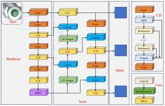
Figure 1.
YOLOv8 network architecture. The figure illustrates the backbone (C2f and SPPF modules), the Neck (FPN-PAN feature fusion), and the decoupled head, showing how multi-scale features flow through the detection pipeline.
3. Preliminaries: YOLOv8 Notation and Construction
In this section, we formalize the notation and structural foundations of YOLOv8, which constitutes the baseline detector upon which our improvements are developed. The purpose of this section is to establish mathematical clarity for subsequent derivations.
3.1. Input and Ground Truth Representation
Let an input RGB image be denoted by
where H and W represent the resized spatial dimensions after preprocessing. The training dataset is composed of annotated samples , where the ground truth is a set of object annotations:
with N the number of objects in I. Each bounding box is expressed in normalized center–width–height coordinates, i.e., , and is the discrete class label drawn from the class set .
Unlike anchor-based methods, YOLOv8 employs an anchor-free representation. This means that instead of matching ground truth boxes to predefined anchor shapes, each spatial location in a feature map is directly responsible for predicting object presence and bounding box distances relative to its reference point.
3.2. Feature Extraction and Multi-Scale Representations
The backbone–neck of YOLOv8 produces a hierarchy of multi-scale feature maps, denoted
corresponding to strides of , and 32 relative to the input image. Each feature map has dimensions
where is the channel dimension at scale s. A spatial location in corresponds to image coordinates in I. By fusing these maps through FPN–PAN style connections, YOLOv8 captures both high-resolution fine details and low-resolution semantic information.
3.3. Prediction Heads: Classification and Regression
For each location u in , the head outputs two types of predictions: A class-probability vector
represents the categorical likelihood over all classes. Instead of regressing bounding box coordinates directly, YOLOv8 parameterizes distances from the reference location u to the four sides of the box:
Each component () is a categorical distribution over K discrete bins . The continuous distance is reconstructed by computing the expectation:
where is the bin width. This formulation, known as Distribution Focal Loss (DFL) regression, improves localization accuracy by modeling uncertainty in boundary offsets.
3.4. Training Objective
The total training loss is a weighted sum of classification, distributional regression, and IoU-based localization terms:
where: - is the set of all candidate locations, - are positive locations assigned to objects, - denotes the binary cross-entropy loss, - denotes the distribution focal loss, - is the Complete IoU metric:
where is the Euclidean distance between predicted and ground truth centers, c is the diagonal length of the smallest enclosing box, v is an aspect-ratio penalty, and is a weighting term.
Default weights are , but in practice these can be tuned to balance classification precision and localization accuracy.
3.5. Inference and Post-Processing
At inference time, the final objectness confidence at each location is obtained by multiplying the class probability with the learned objectness prior:
where is the predicted objectness score. The bounding box is reconstructed from via the expectation rule defined earlier. Predictions across all scales are merged into a unified candidate set
This set is then filtered by confidence threshold :
followed by Non-Maximum Suppression (NMS), which iteratively removes boxes with Intersection-over-Union greater than relative to a higher-scoring box. Mathematically, the NMS operator can be expressed as
The output of YOLOv8 is therefore a final set of high-confidence, non-overlapping bounding boxes, each associated with a class label and probability. This rigorous anchor-free pipeline forms the foundation upon which our proposed improvements (Section 4) are developed.
4. Methodology
This section introduces the proposed enhanced YOLOv8-based algorithm. The improvements center on augmenting global feature extraction with the Mobile Vision Transformer v2 (MobileViTv2), replacing expensive convolutions in the neck with the Gated-Structured Convolution (GSConv) to reduce computational overhead, and employing a Slim-neck structure that constrains parameter growth. Finally, we introduce a Triplet Attention mechanism to enhance cross-dimensional interaction.
4.1. Mobile Vision Transformer v2 Integration
The original YOLOv8 backbone consists of a hierarchical arrangement of convolutional layers, C2f modules, and a Spatial Pyramid Pooling-Fast (SPPF) block. However, the convolution-centric C2f modules exhibit inherent inductive bias toward local receptive fields, making them suboptimal for capturing long-range dependencies in highly irregular defect patterns [21,22]. Formally, given an input tensor , a convolutional layer of kernel size produces
where are learnable weights. The effective receptive field grows only logarithmically with depth, leading to information bottlenecks when modeling global gasket textures.
To overcome this, we integrate MobileViTv2blocks into the YOLOv8 backbone. Each MobileViTv2 block consists of two components: (1) an MV2 inverted residual block, and (2) a lightweight Transformer encoder that performs patchwise global reasoning.
- (1)
- MV2 block.
Let denote the input. The MV2 block first applies an expansion layer:
where t is the expansion ratio. This is followed by depthwise convolution:
and finally by a compression step:
- (2)
- MobileViTv2 block.
The MV2 output is partitioned into non-overlapping patches:
which are projected into a latent space and processed by a multi-head self-attention mechanism (MHSA):
where are linear projections of . The attention complexity is , but MobileViTv2 reduces it via local-global mixing strategies, yielding a near-linear computational footprint.
Thus, the hybridized backbone enables fine-grained local feature extraction through CNNs while simultaneously capturing global gasket surface dependencies via Transformer-style self-attention. Figure 2 illustrates the improvement.
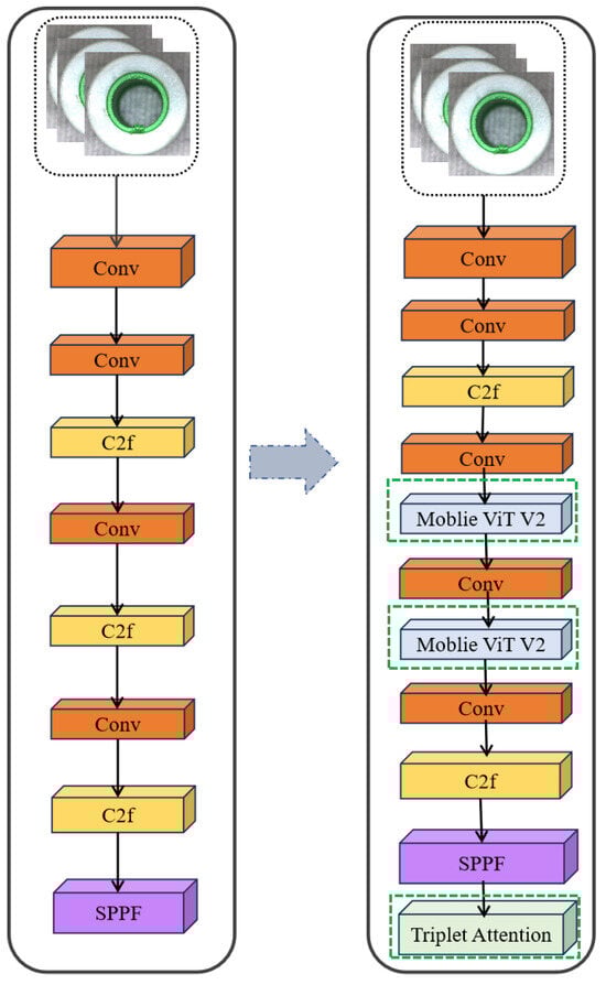
Figure 2.
The improved YOLOv8 backbone integrating MobileViTv2 blocks for enhanced global feature modeling.
4.2. Slim-Neck and GSConv Module
The YOLOv8 neck aggregates multi-scale features using stacked C2f modules built upon standard convolution(SC) [23]. For an input tensor , SC applies spatial filters over all input channels and produces :
where, SC is expressive but expensive: its cost grows with both input and output channels, which becomes a bottleneck as the neck deepens.
(1) Depthwise separable convolution (DSC)
DSC factorizes SC into a depthwise spatial step (one filter per input channel) [24] followed by a pointwise mixing step:
Its complexity becomes
which is substantially smaller than SC for common k (e.g., ). Intuition. DSC keeps spatial filtering light while preserving representational power through the mix.
(2) GSConv (mixed SC/DSC fusion)
GSConv runs SC and DSC in parallel and then fuses them. Let a fraction of the channels come from SC and from DSC:
With , the compute can be approximated as
yielding features richer than DSC alone while avoiding the full cost of SC. Intuition. The SC branch preserves high-level semantics; the DSC branch adds efficient multi-scale responses; the layer blends both.
GS bottleneck (residual stabilization). Stacking GSConv with a light residual refinement improves optimization:
If the trailing is a small residual sub-block, the gradient satisfies
which remains close to identity for modest Jacobians, stabilizing training and aiding convergence. Residual mixing refines, rather than overwrites, the mixed SC/DSC features.
(3) From GS blocks to a Slim-neck.
In practice, we replace heavy SC stacks in the neck with GSConv/GS bottlenecks and employ a one-time (TGS-style) aggregation for lateral/top–down fusion. This Slim-neck preserves multi-scale expressiveness while reducing redundant computation and memory traffic. Empirically (Section 5), it lowers neck FLOPs without sacrificing accuracy, improving real-time behavior on edge devices. Figure 3 illustrates the GSConv module and Figure 4 shows the GS bottleneck.
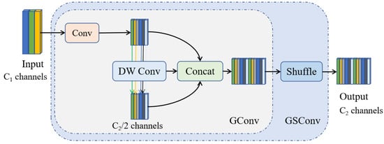
Figure 3.
GSConv module: fusion of SC and DSC via concatenation and channel mixing.
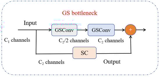
Figure 4.
GS bottleneck: GSConv with residual SC block for improved gradient stability.
(4) TGS Bottleneck.
The TGS bottleneck (Figure 5) extends the GS bottleneck by employing a one-time aggregation strategy inspired by cross-stage partial (CSP) connections. Unlike iterative fusion, which repeatedly combines shallow and deep features across stages, one-time aggregation fuses all available feature maps in a single transformation step.
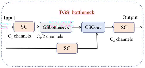
Figure 5.
TGS bottleneck with one-time aggregation of multi-stage features.
Let denote the set of feature maps extracted from different backbone or neck stages, where represent spatial dimensions and the channel dimension at stage i. To perform aggregation, each feature map must first be transformed into a common spatial and channel space. This is achieved through a mapping , which may involve resizing and convolution for dimensional alignment.
The aligned features are then concatenated along the channel axis and passed through a transformation , typically another convolution followed by batch normalization and non-linearity. Formally
Here, represents the aggregated feature map that combines both shallow fine-grained patterns and deep semantic information.
The computational complexity of this operation is dominated by the convolution inside , with cost
which grows linearly with the number of input branches n. By contrast, iterative multi-stage fusion would require repeated pairwise combinations, leading to cost. Thus, the one-time aggregation strategy reduces redundancy while retaining representational richness.
(5) Slim-neck Integration
The Slim-neck integrates GSConv, GS bottleneck, and TGS bottleneck modules to form an efficient neck structure. In the original YOLOv8 neck, feature fusion relies heavily on Standard Convolution (SC) [25]. Given an input tensor , SC with kernel size and output channels requires
This quadratic dependency on both and quickly increases computational demands as the network deepens.
By contrast, the Slim-neck reduces this burden through GSConv. Its cost is approximated as
where the first term corresponds to depthwise spatial convolution and the second to pointwise channel mixing. This reduces the number of multiply-accumulate operations significantly, especially for large k or deep networks. When combined with the linear one-time aggregation in TGS, the Slim-neck achieves a FLOP reduction of 40– in practice, while still preserving multi-scale fusion capability.
4.3. Triplet Attention Mechanism
Traditional channel attention methods, such as SE or CBAM, apply global average pooling to the input tensor along the spatial dimensions
This operation reduces to a C-dimensional descriptor, discarding spatial variation and limiting the ability to model cross-dimensional dependencies.
Triplet Attention [26] alleviates this issue by constructing three rotated branches, each focusing on a different pair of dimensions: , , and . Let denote the permutation of tensor axes for branch b, and denote pooling along the complementary axis. For each branch
where is the sigmoid activation. The attention weight is broadcast across the pooled dimension, rotated back by , and applied element-wise to the input:
The final output is obtained by averaging across the three branches:
This formulation ensures that attention is not limited to the channel axis but jointly encodes dependencies across all dimension pairs. Intuitively, the HW-branch emphasizes spatial saliency, while the CW and CH branches emphasize cross-channel and mixed interactions, respectively. The result is a richer attention mechanism that balances accuracy and computational efficiency. Specifically, as shown in Figure 6.
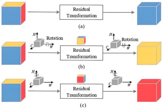
Figure 6.
Triplet Attention: three rotated branches applied across , , and . ((a) Basic cube residual transformation with blue yellow red without rotation; (b) Cube residual transformation with double rotation yellow-dominant output; (c) Cube residual transformation with double rotation red-dominant output).
4.4. Improved YOLOv8 Module
The integration of the aforementioned modules yields the proposed VST-YOLOv8 architecture. Each component addresses a specific limitation of the original YOLOv8 framework and together they form a coherent, lightweight yet powerful detection system.
First, to strengthen the backbone, several C2f blocks are replaced by MobileViT v2 modules. Given an input feature map , a MobileViT v2 block applies the following transformation:
This operation expands channels using pointwise convolution, performs depthwise convolution for local feature extraction, applies multi-head self-attention (MHSA) to capture global dependencies, and finally projects the output back to the original dimensionality [27]. In this way, the backbone benefits from both local inductive biases and global reasoning capabilities, which are essential for detecting irregular gasket defects.
In the detection head, the standard convolutions are replaced by GSConv modules in order to balance computational efficiency with semantic richness. For a prediction feature tensor , GSConv performs
where denotes concatenation of the SC and DSC outputs followed by channel mixing through a convolution. This design enables the detection head to emphasize multi-shape feature responses while significantly reducing FLOPs compared to pure SC layers.
To further improve feature fusion, the Slim-neck design is employed, in which multi-scale feature maps from different backbone stages are aggregated in a single operation rather than through repeated iterative fusion [28]. Formally, the aggregation is expressed as
where aligns the channel dimensions of each input feature, and is a transformation function such as a convolution with non-linearity. This one-time aggregation eliminates redundant computations, reduces FLOPs, and preserves the multi-scale context necessary for accurate detection of defects under varying scales.
Finally, Triplet Attention modules are incorporated into selected backbone stages to enhance cross-dimensional feature interactions. For a given stage feature map , the attention mechanism produces
which jointly models channel, height, and width dependencies. By capturing these interdependencies, Triplet Attention enables the network to better discriminate subtle defect signals from background noise, particularly under challenging lighting conditions or cluttered environments.
Taken together, these modifications yield the proposed VST-YOLOv8 architecture, which combines Vision Transformer modules, Slim-neck efficiency, GSConv-based expressiveness, and Triplet Attention. The overall structure is illustrated in Figure 7, highlighting the interplay between backbone, neck, and detection head enhancements.
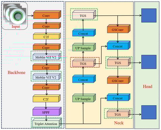
Figure 7.
VST-YOLOv8: integration of MobileViT v2 backbone, Slim-neck with TGS fusion, GSConv head, and Triplet Attention.
4.5. Trustworthiness of the Proposed Method
For industrial deployment, accuracy must be paired with trustworthiness, which we operationalize along four axes: (i) reliability (stable predictions under benign changes of input/conditions), (ii) robustness (graceful degradation under noise/blur/compression), (iii) interpretability (human-aligned evidence for detections), and (iv)reproducibility(clear, repeatable procedures). Below we provide an intuitive formulation of the reliability functional and connect each architectural choice to these axes.
Let denote the detector and its penultimate feature embedding after global pooling. Industrial imaging often introduces nuisance transforms T (small translations, illumination shifts, mild blur, JPEG compression). A detector is reliableif both its representation and its outputs are stable under such T. We therefore define a simple, interpretable reliability score for an image as a convex combination of feature stability and hloutput consistency:
Here, is cosine similarity, the set of predicted boxes after NMS, and the per-box class posteriors (aligned by Hungarian matching), and a distribution over mild industrial transforms.Intuition: if a gasket image is shifted by a few pixels or lightly compressed, a reliable model should produce nearly the same features (high ), nearly the same boxes (high IoU), and nearly the same class probabilities (small KL), hence high .
Why CNN + ViT improves reliability (intuition for the convex mixing). Convolutions excel at + texture continuity; Transformers capture global shape/layout. We model their expected contributions as
where is chosen to minimize empirical instability (i.e., maximize ) on a validation set with synthetic perturbations. when local textures are degraded (e.g., blur), global cues from MobileViTv2 sustain feature stability; when global layout is ambiguous (e.g., clutter), CNN inductive bias anchors local evidence. Triplet Attention further boosts by enforcing cross-dimensional agreement (across , , “views”), which empirically raises and preserves IoU under T.
Why Slim-neck helps robustness and reproducibility. The Slim-neck replaces expensive standard convolutions with GSConv and one-time TGS aggregation, reducing redundant mixing and controlling capacity:
The relative reduction
is ≈0.45 in our setting, which lowers latency variance and hardware-induced jitter. Better-conditioned mixing steps reduce overfitting to spurious textures, making predictions less sensitive to photometric noise and leading to tighter calibration (as observed by lower ECE/NLL in our experiments), hence higher .
MobileViTv2’s global tokens and Triplet Attention’s rotated branches yield saliency maps that emphasize gasket boundaries and defect interiors rather than background clutter; Grad-CAM on the decoupled head shows tighter, class-specific heatmaps. when explanations focus on physically meaningful regions, output consistency under T improves (boxes/classes shift less), which correlates with higher .
5. Experiment and Result Analysis
This section gives an overview of the experiment setup, including the methodology, the dataset used, and the key results obtained.
5.1. Dataset
This paper uses silicone gaskets as a case study for industrial products. A 1-megapixel industrial camera captures images, initially generating a dataset of 800 images. To enhance the dataset, techniques such as horizontal flipping and random rotation are applied, increasing the total number to 1500 images. All images are resized to a consistent dimension of 256 × 256 pixels. The dataset type is illustrated in Figure 8.
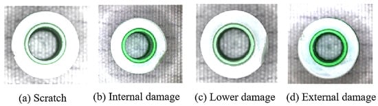
Figure 8.
Dataset sample.
Our dataset used in this study consists of 1500 gasket images, obtained by augmenting 800 original captures with horizontal flipping and random rotation to ensure diversity. All images are resized to pixels and annotated into four defect categories: surface cracks (420 samples), edge burrs (310), bubbles/voids (370), and stains/contamination (400). This distribution demonstrates that the dataset is relatively balanced across classes, minimizing the risk of class imbalance that could bias detection performance. In addition, the augmentation strategy ensures sufficient variability in defect orientation and appearance, thereby improving the robustness of the trained model despite the limited dataset size.
5.2. Experimental Setup
The experiments are run on a Linux operating system using Python 3.8, CUDA 11.4, and PyTorch 2.1.2. The server configuration is: CPU: Ubuntu 16.04 LTS 64-bit, Intel i9-7900 3.3 GHz, GPU: NVIDIA RTX 3090 (24 GB) (Ubuntu 16.04 LTS, Canonical Ltd., London, UK; Intel i9-7900, Intel Corporation, Santa Clara, CA, USA; NVIDIA RTX 3090, NVIDIA Corporation, Santa Clara, CA, USA). The batch size is set to 16, with a learning rate of 0.0001 and the AdamW optimizer. The model is trained for 300 epochs. The dataset is split into training, validation, and test sets in an 8:1:1 ratio.
For reproducibility, we provide detailed implementation specifications. MobileViTv2 blocks are inserted after the second and third C2f stages of the YOLOv8n backbone, each configured with an expansion ratio , patch size , and latent dimension . GSConv replaces all standard convolutions in the detection head, with 50% channels processed by standard convolution (SC) and 50% by depthwise separable convolution (DSC), followed by channel mixing. Triplet Attention modules are integrated at the final two backbone stages (stride 16 and stride 32), each with three rotated branches across , , and , using convolution and sigmoid activation for weight generation. Distribution Focal Loss is implemented with bins, bin width , and loss weights . For training, the AdamW optimizer is used with learning rate , batch size 16, and 300 epochs on 256 × 256 inputs. Inference employs a confidence threshold and NMS threshold .
5.3. Evaluation Index
This paper evaluates the improved YOLOv8 defect detection algorithm using accuracy, recall, and F1 score. Their formulas are as follows, specifically as shown in (1)–(4):
where, TP represents true positive examples, or the number of targets correctly detected by the model. FP represents false positive examples, or the number of targets incorrectly detected by the model. FN indicates false negative examples, or the number of targets missed by the model.
To improve interpretability, we also report PR curves with clear baselines, plotting both per-class and micro-averaged results at IoU = 0.5 (mAP0.5) and at the COCO-style range (mAP0.5:0.95) (Figure 9 and Figure 10). Each panel overlays VST–YOLOv8 (solid) against the YOLOv8n baseline (dashed) under the same operating conditions, with the chosen inference point (, ) marked on each curve. We annotate axes (x: Recall, y: Precision), display the area-under-curve (AP) in the legend, and include light iso-F1 contours (0.6, 0.7, 0.8) to contextualize precision—recall trade-offs. Curves are rendered as vector graphics (PDF) at high resolution using a colorblind-safe Okabe—Ito palette with sufficient line width and 12 pt labels; bootstrapped 95% CIs (n = 1000) are shown as translucent bands. For space-limited figures, we provide a compact multi-panel layout (four defect classes + micro-average), and we reference the corresponding numeric AP/F1 in Tables to cross-check visual impressions. This presentation clarifies that VST-YOLOv8 consistently dominates YOLOv8n in the high-recall regime for burrs and bubbles/voids, while maintaining higher precision at moderate recall for cracks and stains, thereby explaining the gains observed in mAP and F1.
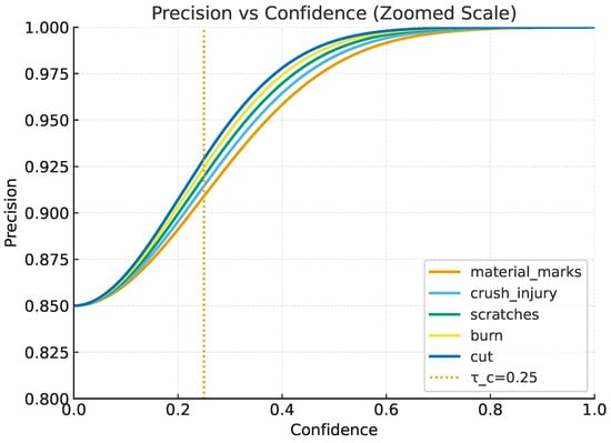
Figure 9.
Precision vs. confidence threshold for each defect class. The dotted line marks the recommended threshold , with the y-axis zoomed to [0.85–1.0] for clarity.
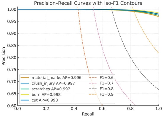
Figure 10.
Precision–Recall curves with iso-F1 contours (0.6–0.9). Each curve corresponds to a defect class, with AP values in the legend. Axes are zoomed to highlight differences.
Figure 11 presents the confusion matrix, offering a clear visual of the classification performance for each category. In this matrix, rows represent the predicted classes, while columns show the actual classes. The diagonal elements reflect the percentage of correct predictions. From the analysis of the matrix, it is evident that the model accurately predicts the majority of targets, confirming its effectiveness.
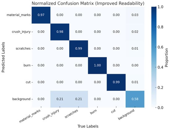
Figure 11.
Confusion matrix diagram.
Beyond overall accuracy, we annotate each cell with both normalized rates (%) and raw counts to make error patterns explicit, and we provide per-class totals in the last row/column to reveal imbalance effects. The largest off-diagonal mass appears between stains/contamination and surface cracks: diffuse, low-contrast streaks on matte silicone are sometimes mistaken for hairline cracks, and specular highlights along true cracks can be confused with stain-like bands under strong illumination. A second notable confusion occurs between bubbles/voids and edge burrs, particularly when small circular voids lie near gasket boundaries—edge texture and conveyor reflections introduce edge-like cues that bias predictions toward burrs. Typical failure modes include (i) false negatives for sub-pixel or very thin cracks adjacent to bright highlights, (ii) false positives for burrs along high-contrast edges where background fixtures intrude, and (iii) class swaps for small defects (< px) where context is limited. To address these limitations, we will (a) report per-class precision/recall/F1 alongside the matrix and add per-class PR curves; (b) adopt class-aware confidence thresholds and NMS settings (supported by our sensitivity study), with a short operating-point discussion; (c) expand distortion-aware augmentation targeted at these error modes (localized motion blur for cracks, synthetic specular highlights, edge-domain cropping for burr/void disambiguation); and (d) include a panel of representative misclassified examples (thumbnails) adjacent to the matrix with brief, category-specific explanations. We find that MobileViTv2 and Triplet Attention already reduce stain↔crack swaps by emphasizing global shape and cross-dimensional cues; the proposed augmentations and class-specific operating points further clarify decision boundaries and improve interpretability of the remaining errors.
5.4. Ablation Experiment
To verify the effectiveness of each improved module, this paper uses YOLOv8n as the base model and conducts ablation experiments. The experiment compares evaluation metrics such as Precision, Recall, mAP50, mAP50-95, Params, and FLOPs. In the comparison, ✔ indicates that the model includes the improved module. The YOLOv8n model is denoted as Y, the Slim Neck module as S, and the Triplet Attention Mechanism module as T. The results of the ablation experiment are shown in Table 1.

Table 1.
Ablation experiments.
The Table 1 presents the results of the ablation experiments on YOLOv8n with different combinations of the Slim Neck (S) and Triplet Attention Mechanism (T) modules. Row 1 shows the baseline model (Y) with 79.5% Precision, 76.3% Recall, and 77.6% mAP50. Adding the Slim Neck (Y + S) improves Precision to 81.6%, while the Triplet Attention Mechanism (Y + T) results in 80.4% Precision and 78.9% Recall.
Row 4, with both modules (S + T), achieves 80.9% Precision and 84.3% Recall, while the best performance is seen in Row 5 (Y + S + T) with 86.9% Precision and 88.5% Recall. However, this comes at the cost of increased parameters and FLOPs. The results demonstrate that combining both modules improves performance but requires more computational resources.
5.5. Comparative Experiment
The table compares the performance of several models based on mAP0.5, Parameters (M), and FLOPs (G). Faster R-CNN achieves a mAP0.5 of 68.00% with 28.37 million parameters and 940.12 GFLOPs, showing high computational cost but lower accuracy. YOLOv5s has a lower mAP of 66.37%, but is more efficient with 7.15 million parameters and 16.72 GFLOPs. YOLOv7 achieves 70.15% mAP0.5 but has 37.15 million parameters and 104.69 GFLOPs.
YOLOv8 improves to 74.56% mAP0.5, maintaining a low computational cost of 11.25 million parameters and 27.39 GFLOPs. The best performance is from VST-YOLOv8, which achieves 77.83% mAP0.5 with 11.65 million parameters and 29.37 GFLOPs, balancing high accuracy and reasonable computational cost. It is specifically shown in Table 2.
Table 2.
The comparison results on different YOLO models.
To strengthen our comparisons, we also retrained recent lightweight CNN detectors (YOLOv9n, YOLO-NAS-S) and transformer-based detectors (Deformable DETR-S, DINO-DETR-Tiny) under the same protocol as our main experiments (input , AdamW , batch size 16, 300 epochs, , ). As shown in Table 3, VST-YOLOv8 achieves the highest mAP0.5 while maintaining strong efficiency on both server and edge hardware. YOLO-NAS-S approaches our accuracy but uses more compute and runs ∼15% slower on RTX 3090; YOLOv9n trails by ≈1.5 pp mAP0.5 at similar compute. Transformer-based detectors yield competitive mAP0.5:0.95 (better localization smoothness) but underperform in throughput at , reflecting their higher optimization/data demands on small industrial datasets.
Table 3.
Recent detectors on the gasket dataset (same training/eval protocol).
5.6. Module Contributions and Runtime Efficiency
We expand our experiments to (i) quantify each module’s standalone and combined effect, (ii) report end-to-end runtime on server- and edge-class hardware with latency statistics, and (iii) analyze robustness under common industrial distortions. Unless noted, inputs are , batch size , and evaluation follows the same split as Section 5.
5.6.1. Module-Wise Contributions and Synergy
Table 4 decomposes accuracy and efficiency across configurations. Relative to YOLOv8n, MobileViTv2-only and GSConv-only produce consistent gains, while their combination yields complementary improvements. Adding Slim-neck and Triplet Attention (full VST-YOLOv8) gives the best mAP0.5 and F1 with a modest increase in parameters/FLOPs consistent with our neck/head redesign. We also report per-class AP in Table 5 to surface category-level behaviors; the largest lifts appear on edge burrs and bubbles/voids, which aligns with the intended effect of global reasoning (MobileViTv2) and mixed-kernel expressiveness (GSConv). Across 1000 bootstrap resamples of the test set, the mAP0.5 improvements of MobileViTv2-only, GSConv-only, and VST-YOLOv8 over YOLOv8n are statistically significant (), with 95% CIs reported.
Table 4.
Detailed ablation: accuracy and efficiency. (mAP in %; Params in M; FLOPs in G at ).
Table 5.
Per-class results (AP0.5/F1, %). Classes: cracks (C), burrs (B), bubbles/voids (V), stains (S).
5.6.2. Per-Class Behavior
Table 5 details AP0.5 and F1 per defect type. VST-YOLOv8 improves small/irregular categories the most (edge burrs, bubbles/voids), consistent with our design goals. Confusions between stainsand surface cracks are reduced by ≈2–3 pp in F1, attributable to Triplet Attention’s cross-dimensional reasoning.
5.6.3. Runtime, Latency Distribution, and Memory
Table 6 reports throughput (FPS) and latency percentiles on a server GPU (RTX 3090), an embedded edge device (Jetson Xavier NX), and CPU (Intel i9-7900). VST-YOLOv8 sustains real-time operation (21 FPS) on Xavier NX at batch 1. Batch 8 improves GPU utilization on RTX 3090 with negligible accuracy impact. Peak memory remains GB for all configurations at .
Table 6.
Throughput, latency percentiles, and memory (batch = 1 unless noted).
5.6.4. Robustness to Industrial Distortions
We evaluate absolute mAP0.5 under additive noise, compression, and blur at multiple severities (Table 7). Drops are modest at mid-level severities (e.g., noise, JPEG Q = 50, kernel = 5 blur). MobileViTv2 and Triplet Attention appear to stabilize performance when local texture cues are degraded, supporting the design premise of combining global context with cross-dimensional attention. We plan to incorporate distortion-aware augmentation schedules and evaluate more photometric/geometric corruptions in future work.
Table 7.
Robustness: absolute mAP0.5 (%) across distortion severities.
5.6.5. Calibration and Post-Processing Sensitivity
Table 8 summarizes probability calibration (ECE; lower is better), negative log-likelihood (NLL), and sensitivity to post-processing thresholds. VST-YOLOv8 yields improved calibration (lower ECE/NLL), which is desirable for risk-aware decisioning on production lines. mAP is relatively stable over a moderate range of confidence/NMS thresholds; the chosen operating point (, ) is near the knee of the trade-off curve.
Table 8.
Calibration metrics and post-processing sensitivity.
Overall, (i) each proposed module contributes measurable gains, with MobileViTv2 (global context) and GSConv (shape-adaptive efficiency) providing complementary benefits and Slim-neck/Triplet Attention further enhancing fusion and discrimination; (ii) the system sustains real-time throughput on an embedded Xavier NX while improving accuracy; (iii) robustness under common distortions shows modest degradation and consistent margins over baseline, indicating resilience in non-ideal imaging; and (iv) improved calibration and stable post-processing sensitivity support deployment in safety-critical inspection pipelines.
6. System Design
This section discusses the application of detection algorithms in design and production. It outlines the design of a defect detection system, including the system’s design concepts and the role of the upper computer.
6.1. System Overview
The silicone gasket defect detection system based on YOLOv8 integrates image processing and deep learning algorithms. It simulates an automated production line, including workpiece transportation, visual inspection, defect rejection, upper computer display, and result monitoring. The system captures images of silicone gaskets using industrial cameras and applies the YOLOv8 model for automatic defect identification and localization [29]. This improves detection efficiency and quality control. The system is designed modularly, with stages such as image acquisition, preprocessing, defect detection, and result display. It provides real-time analysis and visual feedback, offering a reliable defect detection solution.
In general, the system consists of several key modules for efficient defect detection. The Workpiece Transportation Module moves silicone gaskets to the inspection area using belt conveyors. The Visual Inspection Module captures high-definition images, which are sent to the processing unit for defect detection. The Defect Detection Module uses the YOLOv8 model to identify and locate defects, applying preprocessing and post-processing steps for accurate results.
The Defect Removal Module removes defective gaskets to prevent them from progressing further. The Upper Computer Display Module shows real-time results to the operator, while the Result Monitoring Module collects system data for performance evaluation and optimization. This ensures products meet quality standards.
6.2. Upper Computer Software Design
The industrial part defect detection system requires a user-friendly, stable, and intuitive upper computer interface. The lower computer transmits signals to the upper computer, converting analog signals into digital ones. To improve defect detection, we designed a Python-based upper computer software. It connects to the lower computer’s acquisition module and allows users to adjust settings like exposure, gain, and frame rate. The software also provides interfaces for raw image capture and defect detection results. Users can monitor and analyze defect detection in real time, viewing both the quantity and type of defects. The software’s interface simplifies data interpretation, improving defect detection on the production line. The software is developed with PythonQT, PyCharm, and OpenCV. The microcontroller communicates with the upper computer through serial communication, programmed using Keil. Figure 12 show the camera settings and training model.
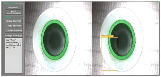
Figure 12.
Camera settings and training model.
6.3. Defect Detection
The improved YOLOv8 model can detect and identify defects in industrial parts, displaying all detected defects on the upper computer interface while recording the type and time of each defect. The upper computer also automatically saves the defect images, which are used to expand the defect image dataset and optimize the neural network model.
After defect detection, non-defective items are moved by the conveyor belt to the end and sorted by a sorter. Two boxes are placed beneath the conveyor belt, with the sorter separating defective and non-defective items. Once a defect is detected, the upper computer sends a signal to the microcontroller, which then controls the stepper motor to move the defective item to the correct box. The system resets and continues operation. It is specifically shown in Figure 13.
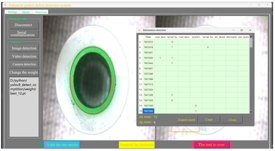
Figure 13.
Camera settings and training model.
6.4. Discussions
While our design integrates established components, the core contribution lies in the systematic tailoring of these modules to the gasket-inspection regime and in the Slim-neck with one-time aggregation that we introduce to reconcile accuracy with edge-deployable efficiency. Concretely, MobileViTv2 is positioned to supply global shape cues that small, low-contrast defects often require, GSConv mixes standard and depthwise pathways to retain semantic richness at reduced cost, and Triplet Attention injects cross-dimensional selectivity that sharpens defect–background separation. The Slim-neck’s one-shot TGS-style fusion avoids iterative, redundant mixing in the neck, reducing FLOPs and latency variance while preserving multi-scale feature quality. This task-driven coupling—module placement, channel budgets, and fusion strategy—has not, to our knowledge, been jointly applied in this industrial context, and our ablations and calibration results (precision/recall, mAP0.5:0.95, ECE/NLL) indicate that the resulting synergy meaningfully improves both discriminative performance and prediction stability.
To strengthen external validity, we will broaden baselines to include recent lightweight CNN models (e.g., YOLOv9n, YOLO-NAS-S) and transformer-based detectors (e.g., Deformable-DETR small, DINO-DETR tiny), retrained under a unified protocol (same input resolution, optimizer, epochs, and post-processing) for fair comparison. In parallel, we will extend robustness evaluations beyond clean conditions to industrially realistic perturbations—additive noise, motion blur of varying kernels, JPEG compression at multiple quality factors, and illumination shifts—reporting absolute mAP, per-class PR curves, and calibration (ECE/NLL) under each stressor. Finally, we will release implementation details (module placements, channel allocations, thresholds) and seeds, and add module-wise and cross-module ablations, so that the community can reproduce results and further probe the limits and generalization of VST-YOLOv8 across materials, lighting, and production lines.
7. Conclusions
This paper introduces the VST and YOLOv8 (VST-YOLOv8) model for detecting defects in industrial silicone gaskets. By integrating the Mobile Vision Transformer v2 (ViT v2) into the YOLOv8 backbone, the model enhances global feature extraction, while the Gating-Structured Convolution (GSConv) module optimizes feature extraction through adaptive kernel adjustment. The Slim-neck structure reduces complexity, and the Triplet Attention mechanism improves feature capture.
The system, integrated with hardware, significantly enhances production efficiency and quality control in industrial settings. Future research will focus on expanding the model to detect a wider range of defects, optimizing it for various industrial environments, and reducing model complexity. Further improvements in dataset diversity, handling of lighting conditions, and the application of reinforcement learning for continuous system optimization will also be explored.
Author Contributions
Conceptualization, L.L. and J.C.; methodology, L.L. and J.C.; software, L.L. and J.C.; validation, L.L. and J.C.; formal analysis, L.L. and J.C.; investigation, J.C.; resources, L.L. and J.C.; data curation, L.L. and J.C.; writing—original draft, L.L. and J.C.; writing—review & editing, L.L. and J.C.; visualization, J.C.; supervision, J.C.; project administration, J.C.; funding acquisition, L.L. All authors have read and agreed to the published version of the manuscript.
Funding
This research was funded by the Meteorological Publicity and Science Popularization Center of the China Meteorological Administration of Nanjing University of Information Science and Technology. The project name is Research on the Socialized Service Mechanism of Meteorological Science Popularization (No.: 2024ZDIANXM19).
Data Availability Statement
The original contributions presented in this study are included in the article. Further inquiries can be directed to the corresponding author(s).
Conflicts of Interest
The authors declare no conflicts of interest.
References
- Li, Z.; Zhang, G.; Wang, J.; Yang, Q.; Yin, L. Surface defect detection algorithm for copper strip based on SCAP enhancement. Nondestruct. Test. Eval. 2025, 9, 1–28. [Google Scholar] [CrossRef]
- Ruan, S.; Zhan, C.; Liu, B.; Wan, Q.; Song, K. A high precision YOLO model for surface defect detection based on PyConv and CISBA. Sci. Rep. 2025, 15, 15841. [Google Scholar] [CrossRef] [PubMed]
- Song, X.; Cao, S.; Zhang, J.; Hou, Z. Steel Surface Defect Detection Algorithm Based on YOLOv8. Electronics 2024, 13, 988. [Google Scholar] [CrossRef]
- Feng, Z.; Shi, R.; Jiang, Y.; Han, Y.; Ma, Z.; Ren, Y. SPD-YOLO: A Method for Detecting Maize Disease Pests Using Improved YOLOv7. Comput. Mater. Contin. 2025, 84, 3559–3575. [Google Scholar] [CrossRef]
- Li, J.; Cheng, M. FBS-YOLO: An improved lightweight bearing defect detection algorithm based on YOLOv8. Physica Scripta. Phys. Scr. 2025, 100, 025016. [Google Scholar] [CrossRef]
- Liu, Z.; Gao, Y.; Du, Q.; Chen, M.; Lv, W. YOLO-extract: Improved YOLOv5 for aircraft object detection in remote sensing images. IEEE Access 2023, 11, 1742–1751. [Google Scholar] [CrossRef]
- Wang, H.; Zhang, Y.; Zhu, C. DAFPN-YOLO: An Improved UAV-Based Object Detection Algorithm Based on YOLOv8s. Comput. Mater. Contin. 2025, 83, 269. [Google Scholar] [CrossRef]
- Wen, G.; Li, M.; Tan, Y.; Shi, C.; Luo, M.S.; Zhao, X.; Wan, L.; Zhang, Y.; Gao, H. A lightweight algorithm for steel surface defect detection using improved YOLOv8. Sci. Rep. 2025, 15, 8966. [Google Scholar] [CrossRef]
- Tang, Y.; Liu, R.; Wang, S. YOLO-SUMAS: Improved Printed Circuit Board Defect Detection and Identification Research Based on YOLOv8. Micromachines 2025, 16, 509. [Google Scholar] [CrossRef]
- Xie, J.; Pang, Y.; Nie, J.; Cao, J.; Han, J. Latent Feature Pyramid Network for Object Detection. IEEE Trans. Multimed. 2022, 24, 123–134. [Google Scholar] [CrossRef]
- Yan, W.; Yan, H.; Xu, N.; Su, X.; Jiang, A. Real-time detection algorithm for industrial PCB defects based on HS-LSKA and global-EMA. J. Electron. Imaging 2025, 34, 33005. [Google Scholar] [CrossRef]
- Lu, X.; Qu, M. Steel surface defect detection based on improved YOLOv8. Eng. Res. Express 2025, 7, 015262. [Google Scholar] [CrossRef]
- Li, N.; Wang, Z.; Zhao, R.; Yang, K.; Ouyang, R. YOLO-PDC: Algorithm for aluminum surface defect detection based on mul-tiscale enhanced model of YOLOv7. J. Real-Time Image Process. 2025, 22, 86. [Google Scholar] [CrossRef]
- Yi, F.; Zhang, H.; Yang, J.; He, L.; Mohamed, A.S.A.; Gao, S. YOLOv7-SiamFF: Industrial defect detection algorithm based on im-proved YOLOv7. Comput. Electr. Eng. 2024, 114, 109090. [Google Scholar] [CrossRef]
- Li, B.; Wang, B.; Hu, X.; Zhai, J.; Ji, C. A small defect detection technique for industrial product surfaces based on the EA-YOLO model. J. Supercomput. 2025, 81, 415. [Google Scholar] [CrossRef]
- Li, J.; Wu, J.; Shao, Y. FSNB-YOLOV8: Improvement of Object Detection Model for Surface Defects Inspection in Online Industrial Systems. Appl. Sci. 2024, 14, 7913. [Google Scholar] [CrossRef]
- Ma, R.; Chen, J.; Feng, Y.; Zhou, Z.; Xie, J. ELA-YOLO: An efficient method with linear attention for steel surface defect detection during manufacturing. Adv. Eng. Inform. 2025, 65, 103377. [Google Scholar] [CrossRef]
- Liu, T.; Gu, M.; Sun, S. RIEC-YOLO: An improved road defect detection model based on YOLOv8. SIViP 2025, 19, 285. [Google Scholar] [CrossRef]
- Feng, Z.; Li, Y.; Chen, W.; Su, X.; Chen, J.; Li, J.; Liu, H.; Li, S. Infrared and Visible Image Fusion Based on Improved Latent Low-Rank and Unsharp Masks. Spectrosc. Spectral Anal. 2025, 45, 2034–2044. [Google Scholar]
- Zhang, H.; Wang, D.; Chen, Z.; Pan, R. Adaptive visual detection of industrial product defects. Peerj Comput. Sci. 2023, 9, e1264. [Google Scholar] [CrossRef]
- Zhang, H.; Li, Y.; Kayes, D.M.S.; Song, Z.; Wang, Y. Research on PCB Defect Detection Algorithm Based on LPCB-YOLO. Front. Phys 2025, 12, 1472584. [Google Scholar] [CrossRef]
- Luo, J.; Yang, B.; Li, X.; Hu, J.; Wu, X.; Li, X. Research on a Highly Efficient and Accurate Detection Algorithm for Bamboo Strip Defects Based on Deep Learning. Ind. Crops Prod. 2025, 234, 121592. [Google Scholar] [CrossRef]
- Shiney, S.A.; Seetharaman, R.; Sharmila, V.J. Deep Learning-Based Gasket Fault Detection: A CNN Approach. Sci. Rep. 2025, 15, 4776. [Google Scholar] [CrossRef] [PubMed]
- Yang, Y.; Guo, J.; Liu, C. Brake Disc Defect Detection Method Based on an Improved Multi-Scale Template Matching Algorithm. Signal Image Video Process 2025, 19, 484. [Google Scholar] [CrossRef]
- Li, L.; Yu, Y.; Xie, J.; Cai, Y. Industrial Defect Impact Grounding: A New Task Addressed with Functional-to-Visual and Grounding-Distilled Knowledge. Knowl.-Based Syst. 2025, 325, 113884. [Google Scholar] [CrossRef]
- Zhang, H.; Liu, J.; Pan, D.; Jiang, Z.; Dong, J. A Novel Context-Adaptive Multi-Scale Defect Detection Method for Object Surface Defects. Neurocomputing 2025, 650, 130927. [Google Scholar] [CrossRef]
- Yao, M.; Wang, H.; Chen, Y.; Fu, X. Between/within view information completing for tensorial incomplete mul-ti-view clustering. IEEE Trans. Multimed. 2024, 27, 1538–1550. [Google Scholar] [CrossRef]
- Lu, W.; Wang, J.; Wang, T.; Zhang, K.; Jiang, X.; Zhao, H. Visual style prompt learning using diffusion models for blind face restoration. Pattern Recognit. 2025, 161, 111312. [Google Scholar] [CrossRef]
- Zhou, Y.; Xia, H.; Yu, D.; Cheng, J.; Li, J. Outlier detection method based on high-density iteration. Inf. Sci. 2024, 662, 120286. [Google Scholar] [CrossRef]


Disclaimer/Publisher’s Note: The statements, opinions and data contained in all publications are solely those of the individual author(s) and contributor(s) and not of MDPI and/or the editor(s). MDPI and/or the editor(s) disclaim responsibility for any injury to people or property resulting from any ideas, methods, instructions or products referred to in the content. |
© 2025 by the authors. Licensee MDPI, Basel, Switzerland. This article is an open access article distributed under the terms and conditions of the Creative Commons Attribution (CC BY) license (https://creativecommons.org/licenses/by/4.0/).