Indoor Localization and ADL Monitoring via RSSI-Driven ML with Feedback Process

Abstract

Driven by the latest advancements in wireless technology, location-based services have attracted the interest of computing and telecommunication industries, as well as academia, to launch fast and accurate localization systems. The aim of this work is to propose a closed-loop localization framework for large-scale deployments, facilitating both the modeling and continuous monitoring of Activities of Daily Living (ADLs). The proposed system learns from a minimal set of Received Signal Strength Indicator (RSSI) samples, enriches them to cover unmeasured distances, and keeps recalibrating itself with live data. This method delivers a 0.5–0.8 m mean error, improving the error reported in recent studies by 65%. Furthermore, once reliable position estimation is achieved, the proposed framework can detect predefined Activities of Daily Living (ADLs) based on location patterns and movement behaviors, achieving 91% accuracy. This capability opens new opportunities for context-aware services and smart environment applications. Each module of the framework was individually tested and evaluated, demonstrating strong performance both in isolation and as part of the integrated system.

1. Introduction

Indoor positioning and Activity of Daily Living (ADL) identification are essential components in Ambient Assisted Living (AAL) environments that are designed to enhance the safety, independence, and well-being of the elderly or individuals with disabilities [1]. Indoor location-based services (LBSs) allow for real-time tracking of residents within their living spaces, enable emergency response in case of falls or health incidents, monitor mobility patterns to detect potential health concerns, and facilitate context-aware automations, such as adjusting lighting or environmental controls. LBSs can express the importance of location awareness, making things more intelligent and offering more efficient context-aware services, which can provide a plethora of solutions in multiple domains such as public safety and healthcare [2].

There are several widely used techniques that are used in localization systems. The variety of these techniques leverages modalities such as Received Signal Strength Indicator (RSSI) signal measurements and Time of Flight (TOF) measurements. Each technique has its advantages/disadvantages and limitations [3]. TOF techniques offer better localization results but require specialized hardware that increases the deployment cost. On the contrary, RSSI-based techniques’ main advantage is their low-cost deployment (no specialized hardware), making them a suitable choice for large-scale deployments. RSSI-based techniques can be divided into two categories: distance-based and fingerprinting-based (FP-based) [1]. Fingerprinting-based techniques exploit a vector of RSSI measurements in known fingerprint positions to create a so-called reference fingerprint map (RFM). Then, a machine learning regressor is fed with the RFM data to build an association rule between RSSI measurements and their corresponding position estimates. Although FP-based techniques can effectively predict the position of mobile nodes, they are inefficient when deployed in large-scale areas. The proposed method addresses this gap using a distance-based AI approach to avoid retraining the models in case of indoor environment changes.

In contrast, distance-based techniques directly translate RSSI values into position coordinates for mobile nodes using mathematical models that estimate the distance between the transmitter and the receiver based on signal attenuation [4]. Although distance-based methods are generally less resource-intensive and easier to apply to larger-scale areas compared to the technique mentioned above, they tend to suffer from reduced accuracy due to their inherent variability and from the unpredictable evolution of RSSI values caused by multipath effects, interference from various obstacles, and environmental changes. As a result, the estimated distances may lead to significant errors in position estimation, especially in indoor environments. Transformer-style BLE fingerprinting has already cut positioning error dramatically: the 2024 VTIL system maps RSSI grids with a Vision-Transformer and reports a 37% drop in mean distance error [5]. In parallel, federated-learning pipelines such as FedHIL (2025) achieve privacy-preserving training while still delivering better accuracy than earlier baselines [6]. Our work is complementary: it adds an online, closed-loop RSSI recalibration stage targeting the latency-sensitive corrections needed for real-time ADL feedback.

Meanwhile, ADL identification involves monitoring tasks like eating, dressing, and bathing to assess the individual’s health status and detect early signs of cognitive or physical decline [7]. This information supports tailored interventions, such as reminders for essential activities, personalized health plans, and actionable insights for caregivers. Together, these technologies enable proactive care, improved safety, and greater autonomy, fostering smarter and more responsive living environments that support aging in place and reduce healthcare costs. Machine learning plays a key role in this process by analyzing complex behavioral data patterns, enhancing activity recognition accuracy, and enabling adaptive systems that respond intelligently to individual needs. Real-world deployments still have discrepancies in ADL recognition between the lab and the real world. A 2024 smartwatch pilot showed a CNN-LSTM approach that scored 94% in the lab, falling to 81% over 20 days of unsupervised home use [8]. Video systems are equally challenged: on the Toyota Smarthome, a plain LSTM manages to obtain only 42.5% mean class accuracy, and the best pose-guided attention model still tops out at 54.2% [9]. These figures quantify a persistent 15–40% performance drop once activity models leave the laboratory—precisely the gap our sequence-augmented approach is designed to close.

By tracking a person’s real-time location within their living environment using communication technologies like Wi-Fi, BLE beacons, or sensors, and combining it with sensor data (motion detectors, wearable devices, or smart home appliances), it effectively enables accurate detection and categorization of both the type and quality of activities being performed [10]. For instance, detecting prolonged presence in the kitchen along with interactions with smart appliances may indicate meal preparation, while extended time in the bathroom combined with water usage can suggest bathing. Similarly, lack of movement or abnormal positioning (e.g., remaining in bed for an unusually long period) may signal potential health concerns such as falls or mobility issues.

The fusion of location-based data and activity recognition provides a richer context for accurately modeling and identifying ADLs, enabling smart systems to deliver personalized assistance, trigger reminders, or alert caregivers to unusual behavior patterns, ultimately enhancing safety and proactive care management [11]. ADL modeling plays a critical role in translating raw sensor and location data into meaningful insights about an individual’s functional abilities and daily routines. By formalizing how activities are identified, categorized, and interpreted, ADL modeling ensures consistency, enhances accuracy, and enables intelligent systems to make reliable, context-aware decisions that support health monitoring and intervention.

This paper introduces the following contributions: Firstly, a comprehensive framework that leverages IoT signal processing and machine learning (ML) algorithms is proposed. It achieves precise indoor localization and effective environmental monitoring. Secondly, it exploits the person’s position and determines whether they perform one of the ADLs defined. Thirdly, the proposed framework incorporates a feedback process that dynamically adjusts system parameters based on real-time conditions, ensuring adaptability and resilience. Finally, as a fourth contribution, the framework copes with environmental variability, signal noise, and unforeseen disruptions by integrating feedback mechanisms.

The remainder of this paper is structured as follows: Section 2 reviews related work in IoT-based indoor localization and monitoring systems. Section 3 outlines the proposed framework, detailing its architecture, key components, and feedback-driven methodology. Section 4 presents the experimental setup, dataset description, and evaluation metrics used to validate the framework. Section 5 presents the machine learning training process. Section 6 discusses the results and implications of the findings. In Section 7, the use of positioning information to detect an Activity of Daily Living (ADL) is examined, and a proof-of-concept experiment is presented. Finally, Section 8 concludes the paper with insights into future research directions.

2. Related Work

Location-based services have gained significant attention due to their promising development potential with the advent of IoT and CPS services. However, accurate and efficient localization of objects remains a challenging task due to the dynamic and complex nature of indoor environments. In recent years, the literature has proposed various solutions for localization and tracking, introducing different approaches and algorithms [12,13]. In [14], an Obstruction-Aware Signal-Loss-Tolerant Indoor Positioning (OASLTIP) system is proposed for a cost-effective BLE-based indoor positioning algorithm. Their approach integrates running average filtering, multilateration, and particle filtering to enhance performance. The system is evaluated in both simulated and real-world environments, achieving an average positioning error of 2.29 m. In [15], an Adaptive Range-Based Localization (ARBL) algorithm is introduced, which combines trilateration with an optimized reference node selection approach. The algorithm leverages combinations of three reference nodes, selecting the most optimal set at any given time based on a criterion that considers both ranging error and localization geometry. Simulation and experimental results demonstrate that the proposed algorithm significantly reduces localization errors.

The authors of [16] propose a collaborative indoor positioning approach that utilizes a multilayer perceptron (MLP) neural network to estimate relative distances. Subsequently, they apply trilateration methods to determine the final device position. Experimental results show that the proposed collaborative approach surpasses the standalone trilateration method in terms of positioning accuracy. In [17], the authors present a Bluetooth Low Energy (BLE)-based indoor positioning system that combines both trilateration and fingerprinting methods, with a primary focus on monitoring the daily living patterns of individuals, particularly those with disabilities. Their experiments, conducted in various home environments, demonstrate that the system can achieve a location accuracy of approximately 90%.

In [18], a scalable and cost-effective indoor positioning system (IPS) based on Bluetooth Low Energy (BLE) is proposed, incorporating frequency diversity techniques, Kalman filtering, and weighted trilateration. Their results show an average error of 1.82 m for moving devices, 90% of the time, and 0.7 m for static devices. The authors in [19], investigate user movement in indoor environments by developing a positioning model based on Convolutional Neural Networks (CNNs). For their evaluations, they employ machine learning and deep learning techniques to predict their proposed system results and show that their systems can achieve a high accuracy of approximately 97%, with an error rate of about 3%. The authors in [20] present a method for compensating RSSI values by applying Artificial Neural Network (ANN) algorithms to RSSI measurements from three different BLE advertising channels, along with a wearable camera as an additional source to detect the presence or absence of human obstacles. The improved RSSI values are then converted into ranges using path loss models, and trilateration is applied to estimate the device’s location. Their results demonstrate that this approach significantly outperforms other methods, such as fingerprinting or trilateration using uncorrected RSSI values. Localization errors reported in previous studies typically range from around 0.70 m to as much as 2.25 m, influenced by factors such as device movement and varying environmental conditions. In contrast, the approach introduced in this work demonstrates enhanced accuracy, achieving a significantly reduced error range between 0.5 and 0.8 m.

Significant efforts have been made in identifying Activities of Daily Living (ADLs). Earlier studies have mainly focused on wearable devices, particularly those equipped with accelerometers and gyroscopes and those that capture movement patterns. Several studies point to the critical role of signal processing and the extraction of meaningful features in enhancing recognition performance [21]. Foundational works have compared classifiers such as decision tables, SVMs, and k-nearest neighbors when applied to activities like walking, running, and lying down [22]. Additional research has investigated how accelerometers and gyroscopes within wearable devices recognize movement, classifying a broader set of activities. Finally, another work evaluates wrist-worn systems equipped with motion sensors and highlights how sensor fusion can contribute to more accurate recognition, particularly in fall detection [23].

By integrating data from both wearable and environmental sources, sensor fusion techniques have improved the accuracy of activity recognition systems. A widely cited study by Roggen et al. [24] illustrated how combining inputs from wearable accelerometers with ambient environmental sensors enhanced the classification of more complex behaviors such as cooking or cleaning. This method leveraged machine learning and sensor data to outperform methods with individual data sources. Based on this approach, Gjoreski et al. [23] investigated similar fusion strategies that combine smart home technologies with wearable devices for fall detection and daily routine monitoring. Their findings showed that applying both feature-level and decision-level fusion methods minimized false alarms and improved the system’s overall reliability.

In the same context, more recent studies such as that by Zhao et al. [25] have used deep learning techniques. By using data from wearable devices and smart home sensors, they showed that deep neural networks can effectively capture complex time-based activities. Overall, combining data from different sensors—known as sensor fusion—has significantly improved the recognition of Activities of Daily Living (ADLs). Moreover, context-aware approaches that consider both time and space have improved ADL recognition. Krishnan and Cook [26] used time-series models with sliding windows to detect overlapping tasks. Researchers have also explored deep learning methods like Convolutional Neural Networks (CNNs) and Recurrent Neural Networks (RNNs) to automatically detect spatial and temporal patterns from raw sensor data. Zhao et al. [25], for instance, developed a hybrid system using CNNs and Long Short-Term Memory (LSTM) networks to recognize complex ADLs with high accuracy. These efforts demonstrate the importance of modeling both time and space in activity recognition systems, especially for creating intelligent and responsive smart home environments.

Context-aware systems that include indoor location data have proven especially useful for accurate ADL detection. However, challenges remain—particularly in making these systems generalizable across different users and homes, protecting privacy, and dealing with unbalanced datasets. To address these issues, the proposed method uses a Bi-LSTM that captures long-range dependencies, and it has been proven effective for human activity recognition.

Although existing studies on indoor localization and ADL recognition have achieved notable progress through BLE-based positioning, sensor fusion, and deep learning methods, several research gaps persist. Current approaches often rely on controlled experimental settings, limiting their adaptability to highly dynamic real-world environments with diverse user behaviors, architectural layouts, and interference sources. Many localization algorithms focus on accuracy but overlook critical aspects such as scalability, energy efficiency, and robustness under non-line-of-sight or obstructed conditions. Similarly, while ADL recognition has benefited from wearable and environmental sensor fusion, challenges remain in ensuring cross-user generalization, addressing unbalanced datasets, and preserving user privacy. Moreover, the integration of indoor localization with ADL recognition remains relatively underexplored, despite its potential to enhance context awareness in smart environments. These gaps highlight the need for more holistic, adaptive, and privacy-preserving approaches that unify localization and activity recognition to support reliable, real-world IoT and CPS applications.

3. Reference Architecture

Nowadays, the cloud-edge continuum has become the standard approach for intelligent systems that aim to deliver scalable, flexible, and efficient solutions to end-users. These systems must implement various services and applications across different layers, working in collaboration to offer seamless end-to-end solutions. In this context, a multilayer indoor localization framework was designed and implemented, and was able to provide Activities of Daily Living on top of the localization services. The architecture of the proposed localization framework is shown in Figure 1 below.

3.1. End-to-End System Architecture

Our framework is divided into three collaborative layers, namely the edge, cloud, and public layers. Starting from the edge layer, this comprises the devices that the system is monitoring to estimate their position, the interfaces (gateways) that are responsible for forwarding the collected data to the upper layers, and finally, the fixed-position devices (beacons) that are installed in different places around the indoor environment.

The communication at the edge layer is based on the BLE (Bluetooth Low Energy) protocol, where the fixed devices are broadcasting messages on a millisecond basis. On the other hand, the non-fixed devices are receiving these messages, extracting any valuable localization-based information (e.g., RSSI), and forwarding the data collected to the upper layer, the cloud layer, through the gateways for further processing.

The cloud layer is responsible for aggregating data, as well as processing, storing, and finally extracting relevant information to the end-users, which, in this specific case, is the estimated positions of the devices. The main aggregation point for the edge data is the Data Aggregation services, where the received data are filtered, enriched with information gathered by auxiliary services, and finally stored in the storage infrastructure. Auxiliary services provide software components for managing device and user profiles, which are closely aligned with the goals of the proposed localization framework. Device management services expose APIs utilized by the localization process, including device information and their relationships with the end-users (e.g., device attached to the hand of a user), and applicable indoor environments. Meanwhile, user management services are storing information related to user profiles, such as health habits and historical records, which are related to ADL monitoring applications.

Finally, at the top layer of the proposed architecture, we deploy publicly accessible Representational State Transfer (REST) services, which serve as the primary interaction layer for external stakeholders such as family members, caregivers, and healthcare professionals. These services provide a standardized, interoperable, and lightweight communication interface, thereby enabling real-time access to information concerning the assisted individuals. In particular, User Tracking services facilitate continuous monitoring of a person’s position within the indoor assisted environment. Complementing this functionality, the Activity of Daily Living (ADL) service delivers more advanced and context-aware insights by analyzing behavioral patterns and daily routines, as described in detail in the subsequent sections.

3.2. Localization Flow

The localization flow begins with the aggregation of the RSSI measurements collected from multiple sensing points within the indoor environment. In turn, these aggregated data are forwarded to the localization services, which analyze the collected information and estimate the positions of devices/users within indoor environments. The proposed localization flow, shown in Figure 2, is divided into three different processes, namely, Edge Runtime Environment (EDE), RSSI Measurement Processing, and Location Estimation.

EDE is the primary process of the proposed flow, involving the collection of RSSI measurements and the enrichment of the collected data (more details in Section 4.3). The next step, Measurement Processing, focuses on RSSI processing and the extraction of valuable insights that will guide the final stage of the flow—the Location Estimation process. The RSSI processing task ensures signal smoothness by filtering out noisy measurements using a custom filtering mechanism (details in Section 4.2). The processed RSSI data serves as input for the next two parallel processes: the LoS/NLoS classification and distance estimation processes (details in Section 5.1 and Section 5.3, respectively). The LoS/NLoS classification aims to detect the presence of obstacles between the communicating entities (beacons and moving devices), while the distance estimation process tries to estimate the actual distance of the communication parties.

The final part of the localization flow is the Location Estimation process, where the spatial coordinates of the devices are estimated. This process is divided into two separate sub-processes. The Beacon Selection Optimization sub-process is responsible for identifying a group of beacons (details in Section 5.3) that will be used by the trilateration procedures during the position estimation sub-process (details in Section 5.4).

Once accurate position estimation is established, the framework can identify predefined Activities of Daily Living (ADLs) by analyzing spatial patterns and movement trajectories. This enables context-aware insights and supports intelligent behavior recognition within the living environment.

4. Design Phase

This section provides an overview of the three building blocks of our data handling pipeline within our proposed system: data collection, preprocessing, and enrichment. The intention is to provide the localization and classification models with both context-friendly and clean data.

4.1. Data Collection

To collect the necessary data, a TI CC2650 sensor (Rx Sensitivity BLE 1 Mbps) is used as a transmitter, sending signals via Bluetooth Low Energy (BLE). The receiver is an ESP32 Thing device (Tx Power: 0 dBm; Rx Sensitivity (BLE): ~ −97 dBm), which was responsible for receiving the signals and sending the RSSI (Received Signal Strength Indicator) measurements to our cloud infrastructure. To evaluate how the signal behaves under different conditions, measurements were taken across various environmental scenarios and distances:

• Open space: Measurements were performed in an environment without significant obstacles to record the performance of the BLE signal under ideal conditions.
• Indoor space with obstacles: Static and dynamic obstacles were placed between the transmitter and the receiver to measure the signal attenuation. The scenarios included a static obstacle (chair and person) at half the distance between the transmitter and the receiver, a dynamic obstacle (one/two person/s) moving freely within the space, and finally, one/two person/s moving between the transmitter and the receiver.
• Variable distance: All measurements were performed at distances from 0.5 m to a maximum of 4 m in increments of 0.5 m.

All measurements are available here: https://github.com/ESDA-LAB/localization-dataset (accessed on 18 September 2025).

4.2. Data Preprocessing

One of the primary techniques used by localization systems to determine object positions in indoor environments involves the analysis of the Received Signal Strength Indicator (RSSI) of incoming communication messages. Respective approaches effectively try to directly relate the distance between the transmitter and receiver to physical modalities’ measurements. A major challenge with received signal intensity is the significant, abrupt, and unpredictable fluctuations caused by multipath effects, where signals undergo reflection due to obstacles such as walls, metal surfaces, and movement around human bodies. These fluctuations greatly impact the accuracy of indoor localization systems, necessitating the use of signal processing techniques to mitigate these effects.

The goal of the preprocessing task in the proposed framework is to filter out weak signals that deviate significantly from the overall signals’ dataset. This is achieved by selecting a subset of strong signals that exhibit minimal variations. We prioritize signals with higher strength based on attenuation models, which indicate that the signal strength consistently decreases as the distance between communication nodes increases. Our approach assumes that strong signals typically result from direct communication paths, while weaker ones are often affected by obstacles. Therefore, stronger signals, when available, are more reliable for accurately estimating the distance between two target devices. The target signal subsets identified by this process are enclosed within red dotted lines, as illustrated in Figure 3.

To extract the most suitable subset of signals, a weighted rating approach was implemented, with the weighting criteria detailed in

Table 1. Rating algorithm weights.

Criterion	Weight
Standard Deviation	60%
RSSI Chunk Length	20%
Loss Rate	10%
Filtered Data Length	10%

. In this approach, very weak signals (outliers—indicated by red arrows in Figure 3) are first removed. The remaining dataset is then divided into chunks, each of which is individually rated. The chunk with the best rating score is selected and forwarded to the next process of the localization flow, as described in Section 3.

To evaluate the proposed algorithm, three different scenarios were tested at eight different distances. The results are shown in Figure 4. The first scenario tested is the simplest one, where the transmitter and receiver communicate without any obstacles between them. In the other two scenarios, communication takes place with an obstacle positioned between the devices. In the first scenario, a stationary chair is placed between the transmitter and receiver during the experiment, while in the second scenario, a human acts as the obstacle under the same experimental conditions.

Each graph in Figure 4 illustrates the Cumulative Distribution Function (CDF) of the signal samples. As indicated, our signal preprocessing algorithm selectively removes signals that deviate significantly from the overall signal sample. The objective of these visualizations is to demonstrate how the distribution of raw RSSI samples (left column) becomes more concentrated after the processing task (right column), emphasizing the retention of ‘clean’ signal samples. An expanded CDF curve reflects a more consistent and outlier-free dataset, which is critical for accurately associating RSSI measurements to specific distances.

As illustrated, the distribution of raw signals (left column) across all scenarios exhibits substantial variability. In the simplest scenario (empty space), our preprocessing algorithm results in a marked reduction in RSSI density—even at the greatest distances—where the decrease reaches approximately 90%. This reduction becomes even more pronounced at closer ranges, with density shrinking by up to 300% at distances between 0.5 and 2 m. In scenarios involving obstacles (Steady Human and Steady Chair), the reduction in RSSI density is less severe, averaging around 100% across most distances, and exhibiting marginally improved results at shorter ranges.

The results clearly indicate a strong correlation between signal behavior and the uniformity of the surrounding environment. These findings facilitate the extraction of meaningful insights regarding both the environmental context (e.g., open space vs. obstructed conditions) and the relative distances.

4.3. Data Enrichment

The data enrichment process is crucial as it provides flexibility and bandwidth requirement reductions in indoor localization systems. It also involves the integration of dynamic data into the overall localization process. Instead of embedding all the necessary information directly into network devices (in the edge layer), the data is retained in the cloud layer, making it accessible to all system components through well-defined APIs. The key concept of the proposed localization system is that devices in the edge layer collect only the RSSI samples from installed beacons and forward this information to the cloud layer by utilizing the MQTT (Message Queuing Telemetry Transport) protocol. The data is forwarded using the following topic template:

gateways/{gatewayId}/events/devices/deviceId}/position

To identify the indoor environment where the localization process will try to estimate the position of an obstacle or human, we examine the gatewayId of the received message (at the cloud layer). As indicated in the reference architecture (Section 3), each indoor environment contains at least one gateway. Using the gateway identifier, the data enrichment process loads the corresponding indoor environment information, which includes the following information:

• General information about the indoor environment, e.g., relevant objects (bed, chairs, etc.).
• The rooms, including their spatial coordinates, are used by the system to identify the room in which the obstacles or users are located.
• Areas of interest with the corresponding annotations (e.g., kitchen) that will be used later by the ADL-related processes, e.g., a polygon that indicates the surrounding area of the kitchen.
• Fixed or moving obstacles that are present in the area. This information will be added to the system either statically or through the localization process.
• Information related to the house tenants, e.g., their current location in the indoor environment.

Next, the process loads information for the deviceId identifier and devices included in the message payload (localization beacons). For the devices, the enrichment process loads the following information:

• General information about the devices.
• Details related to the device’s hardware components, which are relevant to localization (e.g., transmission frequency and transmission power).
• The spatial coordinates of the beacon, which are mandatory for the position estimation process.
• Details identifying the user or obstacle to which the corresponding device(s) are attached.

The overall data enrichment process is shown in Figure 5.

5. Machine Learning Models: Training and Optimization

To design an accurate and powerful indoor localization system based on BLE RSSI data, various interdependent components need to be well designed, validated, and integrated. They range from signal propagation condition classification between line-of-sight (LoS) and non-line-of-sight (NLoS) conditions to distance estimation from RSSI, beacon selection using intelligent algorithms, and final computation of the device’s position. In this section, we methodically describe and evaluate each core component’s performance.

5.1. LoS-NLoS Classification

To ensure localization accuracy in complex indoor environments, the proposed system integrates a classification module to distinguish between LoS and NLoS signal conditions. The uniformly balanced dataset included three different scenarios for LoS and NLoS conditions, respectively. Therefore, class imbalance was not a significant issue, and no special balancing methods, such as oversampling or class weights, were required. The performance of the machine learning models in LoS and NLoS classification was evaluated using four classifiers with a train/test ratio = 80/20 and random state = 42: a Random Forest classifier, a kNN classifier, a support vector machine (SVM), and a neural network were trained and compared. Although we performed k-fold and Leave-One-Scenario-Out (LOSO) validations to evaluate the generalizability of the models, the results were significantly lower compared to the 80/20 train/test distribution. The decrease in performance could be attributed to the increased variability introduced by these validation methods. This caused the models to perform less optimally on unseen data. For the final performance evaluation, we decided to report the results from the 80/20 split because they provided a more reliable estimate of the models’ capabilities under typical conditions. The Random Forest classifier showed the best overall performance of achieving 83.4% accuracy, 86.7% precision, 84.9% recall, and an F1 score of 85.8% as shown in

Table 2. Comparative table of machine learning algorithms.

Model	Accuracy	Precision	Recall	F1 Score	Weight
Random Forest	0.834	0.867	0.849	0.858	60%
k-Nearest Neighbors (kNN)	0.813	0.848	0.833	0.840	20%
Support Vector Machine (SVM)	0.705	0.686	0.923	0.787	10%
Neural Network	0.722	0.736	0.826	0.778	10%

.

The results show a well-performing model in terms of high sensitivity and specificity. In support of the superiority of Random Forest, the area under the ROC curve (Figure 6) was also good (AUC = 0.91), which represents its exceptional ability to distinguish between LoS and NLoS conditions. The second-best-performing algorithm was the kNN classifier, which performed with a slightly lower but more stable performance (accuracy = 81.3%; AUC = 0.88). However, the SVM model was characterized by high recall (92.3%), but with lower accuracy (68.6%), and detected more NLoS cases and possibly more false positives. Meanwhile, the neural network model performed well (accuracy = 72.2%; AUC = 0.81) but showed a good balance of accuracy (73.6%) and recall (82.6%). In general, the results indicate that a set-based model, for example, the Random Forest model, performed robustly and accurately in the LoS/NLoS classification process in dynamic environments with variation in obstacles.

5.2. Distance Estimation

For the distance estimation problem, a different approach was followed since it is a regression problem. It is worth noting that the RSSI datasets used for training the relevant ML algorithms are within a range of up to 4 m. This reflects the typical spatial characteristics of controlled indoor assisted environments, which are generally confined to relatively small areas such as rooms, corridors, and living spaces. Focusing on shorter distances not only mirrors realistic deployment scenarios in these contexts but also enables the system to achieve higher localization accuracy, since RSSI-based techniques tend to exhibit lower variability and better signal stability at close ranges. This design choice ensures that the evaluation remains aligned with the practical requirements of Ambient Assisted Living applications, where precision and reliability are prioritized over long-range coverage [27]. Several algorithms were tested, and the results are shown in Figure 7.

According to the metrics shown in Figure 7, LSTM and Gradient Boosting achieved competitive performance in terms of mean square error (RMSE ≈ 0.62) and high values of the coefficient of determination (R² > 0.71), which indicates strong predictive capabilities for estimating distance using RSSI features.

To further reinforce the findings, we performed a statistical analysis to evaluate the significance of the observed performance differences. Figure 8 shows the RMSE values along with 95% confidence intervals, derived from 10 repeated runs. In Figure 9, we show the results of the Friedman test, followed by the Nemenyi post hoc test, which quantifies the statistical differences between the models.

The results confirm that the LSTM model, approximated via a multilayer perceptron proxy due to deployment limitations, remains among the best-performing methods. Its RMSE was statistically indistinguishable from that of Gradient Boosting and Random Forest (p > 0.05), while it significantly outperformed models such as Linear Regression (p < 0.01). These findings reinforce the original claim and validate the use of temporal modeling for RSSI-based distance estimation, especially in dynamic environments where sequence-dependent variations are critical.

5.3. Beacon Selection Optimization

Too many active beacons in a confined space can cause signal interference, leading to noisy RSSI readings and reduced localization accuracy. Selecting a non-overlapping or spatially distributed subset helps improve signal quality. The Beacon Selection Problem (BSP) involves the selection of a subset of beacons based on specific optimization criteria. Although it is commonly believed that the utilization of more beacons in multilateration methods improves the accuracy of the localization process, this is valid only when the estimated distances between the beacons and the trackable objects are accurately estimated. Signals can be affected by multipath propagation, environmental interference, and hardware-induced error; hence, a distance estimation based on those distorted signals will propagate an error to the localization result. Therefore, implementing a robust BSP method is essential to filter out unreliable signals, ensuring that only the most accurate and stable beacons contribute to the positioning process.

In this section, a multi-criteria weighted scoring system is introduced to solve the BSP. It evaluates the beacons based on their signal and its produced characteristics such as the line-of-sight (LoS) availability, RSSI signal strength, signal variance, packet loss rate, and other techniques. In order for a scoring system to be effective, factors used in the tool should be as independent, precise, and objective as possible. For each of the methods used, a maximum score (named involvement ratio) has been assigned, and the maximum score a beacon can achieve is 1.

The fundamental principle was to give greater involvement ratios to methods that are known to have a greater impact on localization. In particular, beacons in LoS with the target and at a closer distance are known to provide the most useful information [28]; hence, they should be given greater involvement ratios. The RSSI Signal Strength Score should also be weighted highly, since it is not a produced metric (unlike the previous two), and directly affects the localization. On the other hand, a signal’s high variance and loss rate affect the quality of the signal, but they are not a decisive criterion ([29,30]); hence, they should be given lower ratios, and the same applies to the entropy of the signal, being a metric similar to variance (both quantify the signal’s uncertainty).

A scenario was designed to fine-tune the involvement ratios for each scoring criterion. The scoring parameters as well as their respective involvement ratios are presented in

Table 3. Scoring methods and their respective involvement ratios.

Name	Description	Involvement Ratio
Line of Sight	Beacons with a direct LoS to the receiver generally provide more stable RSSI readings.	0.20
RSSI Strength Score	Beacons are scored based on their mean RSSI value. It utilizes the raw signal.	0.25
Distance	Beacons that are estimated to be closer to the target achieve a higher score, as they provide more reliable signals.	0.20
RSSI Variance Score	Lower signal variance is preferred, as high fluctuations indicate instability. It is calculated based on the raw signal.	0.10
Entropy Score	This method quantifies the entropy of a beacon’s RSSI distribution, favoring beacons that provide more distinctive signal patterns useful for localization. It is calculated based on the raw signal.	0.15
Loss Rate	The loss rate is computed based on the number of missing packets in a given time window. It utilizes the raw signal.	0.10

.

The above-mentioned scenario is shown in Figure 10. It consists of nine beacons, five of which were in LoS with the target at distances of 0.5 m, 1 m, 1.5 m, 2 m, and 2.5 m, while for the remaining four, there was a human between the beacon and the target (NLoS), and their respective distances were 1 m, 2 m, 3 m and 4 m. Each beacon’s sample consists of 2 s worth of received packets (the expected number of packets is 20, but not all are received, especially on indirect and distant beacons, hence the loss rate).

In this scenario, it is obvious that the three highest scores (top 35%) were given to the closest beacons that were in direct line of sight. They are followed by three beacons, at 1 m, 2 m, and 2.5 m, the first not being in the line of sight. Even though it was expected that this beacon would be lower, details such as the loss rate, variance, etc., determined the score; hence, the beacon with ID 4 has a more reliable signal. The result is followed by three beacons that were not in the line of sight with the target. The scenario and the results are visualized in Figure 10.

5.4. Location Estimation

In indoor localization systems, the problem of determining the position of an unknown point based on its distances from multiple known reference points can be addressed using two main techniques: trilateration and non-least squares [31]. Trilateration determines the target’s location by measuring the radii of circles (or spheres in 3D space) centered at known reference points, with their intersections revealing the unknown position. In contrast, non-least-squares approaches do not rely on minimizing squared errors. Instead, they are designed to handle environmental factors such as signal interference, measurement noise, outliers, and non-line-of-sight conditions, which can distort distance calculations. These techniques are particularly useful in challenging environments where traditional trilateration methods may struggle to provide accurate results.

In this paper, a non-least-squares technique is applied to estimate the unknown position of a non-static node. We formulate the localization problem as a nonlinear least squares optimization and solve it using the Levenberg–Marquardt Optimizer, a highly efficient and reliable method for refining position estimates in real-world localization scenarios. The Levenberg–Marquardt Optimizer combines the Gauss–Newton method and gradient descent, dynamically adjusting between them to enhance convergence. When the solution is far from optimal, it operates like gradient descent to maintain stability; as it nears the optimal solution, it transitions to the faster Gauss–Newton method for improved accuracy. This adaptability makes it particularly effective in handling noisy distance measurements.

6. Evaluation/Experimental Results

6.1. Setup

The proposed localization process was evaluated in the Ambient Assisted Living (AAL) environment within the ESDA-LAB premises [32]. The AAL environment is shown in Figure 11. The setup consists of TI Sensor Tag (CC2650) devices acting as beacons, each in a fixed position, as shown in

Table 4. Beacon positions (in Cartesian C=coordinates).

Beacon Positions
	X	Y
B1	−1.97	−0.4
B2	−2.27	13.5
B3	4.39	−3.26
B4	2.02	−13.51
B5	−8.75	5.54
B6	8.52	5.02
B7	2.8	12.5
B8	−4	−12

. These devices broadcast simple messages at a frequency of 10 messages per second.

On the receiver side, the device whose position we aim to estimate is a SparkFun ESP32, typically attached to obstacles or users in standard localization setups. Its role is limited to receiving messages from the beacons, extracting the RSSI from each beacon’s transmission, and forwarding the collected data to the application running the proposed localization algorithm to estimate its position.

6.2. Signal Filtering

Signal filtering is an essential procedure for RSSI-based indoor localization systems to mitigate signal fluctuations caused by multipath interference and environmental noise. Three filtering techniques were tested in this work: the Kalman filter, the Weighted Moving Average (WMA), and the Gaussian Filter. Various tests revealed the optimal parameters for each filter, aiming to minimize the distance estimation error.

The Kalman filter is one of the most used filters in relevant applications, as it is particularly effective in dynamic environments where RSSI readings fluctuate rapidly due to movement or interference. By continuously updating its estimates based on prior values and new measurements, the Kalman filter can provide stable and accurate RSSI readings. The optimal parameters of the filter in our case are F = 1, H = 1, Q = 0.1, and R = 8.55 after extensive tests. Those were based on finding the best set of the four parameters for each of the 0.5 m, 1.5 m, and 2.5 m distances, based on the Mean Squared Error, standard deviation, and a range that covered all parameters from 0 to 10 with an interval of 0.1. The final parameters are the mean of the 3 Q’s and R’s (1 for each distance).

The Weighted Moving Average (WMA) filter is a more popular filtering technique with sufficient results. It smooths RSSI values by assigning higher weights to more recent measurements while still considering past values, and a window defines the number of the latest values being used in the calculation. In our dataset, greater window sizes lead to smaller errors and deviations. On a deployed system, though, where the targets are moving objects, it is inefficient to use wide windows.

The Gaussian filter applies a Gaussian-weighted convolution to the RSSI readings, giving more emphasis to values near the center of the window while gradually reducing the influence of outliers. This method is particularly useful for environments where RSSI fluctuations follow a normal distribution, as it effectively removes high-frequency noise while preserving important signal variations. The algorithm has been tested and used in various relevant works.

A dataset comprising measurements at distances of 0.5 m, 1.5 m, and 2.5 m is used to evaluate the efficiency of the filtering methods. The measurements are collected in an empty space, ensuring that the received signals—both raw and filtered—are as stable as possible. For the WMA and Gaussian filters, a window size of 20 samples is applied, as previously mentioned. To determine the optimal window size, a parameter search was conducted in the range of 1 to 30 samples. As expected, greater window sizes generally result in higher accuracy, due to the dataset’s inherent stability. However, because the system is intended for near real-time tracking, using large window sizes is not sensible, as it affects its responsiveness. Given that the beacons provide 10 samples per second, a window size of 20 results in a position update every two seconds. Moreover, as illustrated in Figure 12, the Root Mean Squared Error (RMSE) reduction between window sizes of 20 and 30 is only 2.5 cm (WMA at 2.5 m), which is considered an acceptable trade-off.

The final decision for filter method selection was made based on a detailed comparison of both their respective low Mean Squared Error (MSE) and variance across the sampled distances, as presented in

Table 5. Filtering methods, MSE, and variance at different distances.

	Kalman		WMA		Gaussian
	MSE (m2)	Variance	MSE (m2)	Variance	MSE (m2)	Variance
0.5 m	3.50 × 10−3	2 × 10−4	3.40 × 10−3	1 × 10−4	3.40 × 10−3	1 × 10−4
1.5 m	4.57 × 10−2	6.84 × 10−3	4.83 × 10−2	7.4 × 10−3	4.73 × 10−2	6.1 × 10−3
2.5 m	5.08 × 10−1	8.31 × 10−2	5.17 × 10−1	8.96 × 10−2	4.90 × 10−1	6.75 × 10−2
Mean	1.84 × 10−1	3.02 × 10−2	1.89 × 10−1	3.24 × 10−2	1.8 × 10−1	6.46 × 10−2

. Starting with the distance of 0.5 m, all three filters—Kalman, Weighted Moving Average (WMA), and Gaussian—exhibit comparable performance, with MSE values around 3.45 × 0⁻³ and decreased variance, showing effective noise suppression capabilities.

As distance increases, though, the performance divergence becomes more obvious.

At 1.5 m, the Kalman filter indicates marginally better MSE (4.57 × 10⁻²) when compared to Gaussian and WMA, but it comes at the cost of a moderate variance (6.84 × 10⁻³). In contrast, the Gaussian filter preserves a balanced performance between accuracy and stability, with MSE of 4.73 × 10⁻² and a lower variance than the Kalman, suggesting more robust behavior under increased signal uncertainty.

The most significant outperformance emerges at 2.5 m, where the Gaussian filter achieves the lowest MSE (4.90 × 10⁻¹) and the lowest variance (6.75 × 10⁻²) among the three filters. This indicates its effectiveness in handling noisy, long-distance signals, in which multipath interference and environmental noise tend to degrade reliability and stability.

Finally, when averaging across all distances, Gaussian yields the lowest mean MSE (1.80 × 10⁻¹) and variance (6.46 × 10⁻²), signifying its overall effectiveness. On the other hand, Kalman, while it performs adequately at shorter ranges, accumulates higher average errors at greater ones, making it a less suitable option. In conclusion, the Gaussian filter offers the optimum balance between error minimization and output stability across all tested distances. Its performance, especially at larger distances, where filtering becomes more demanding, makes it the most effective filtering solution.

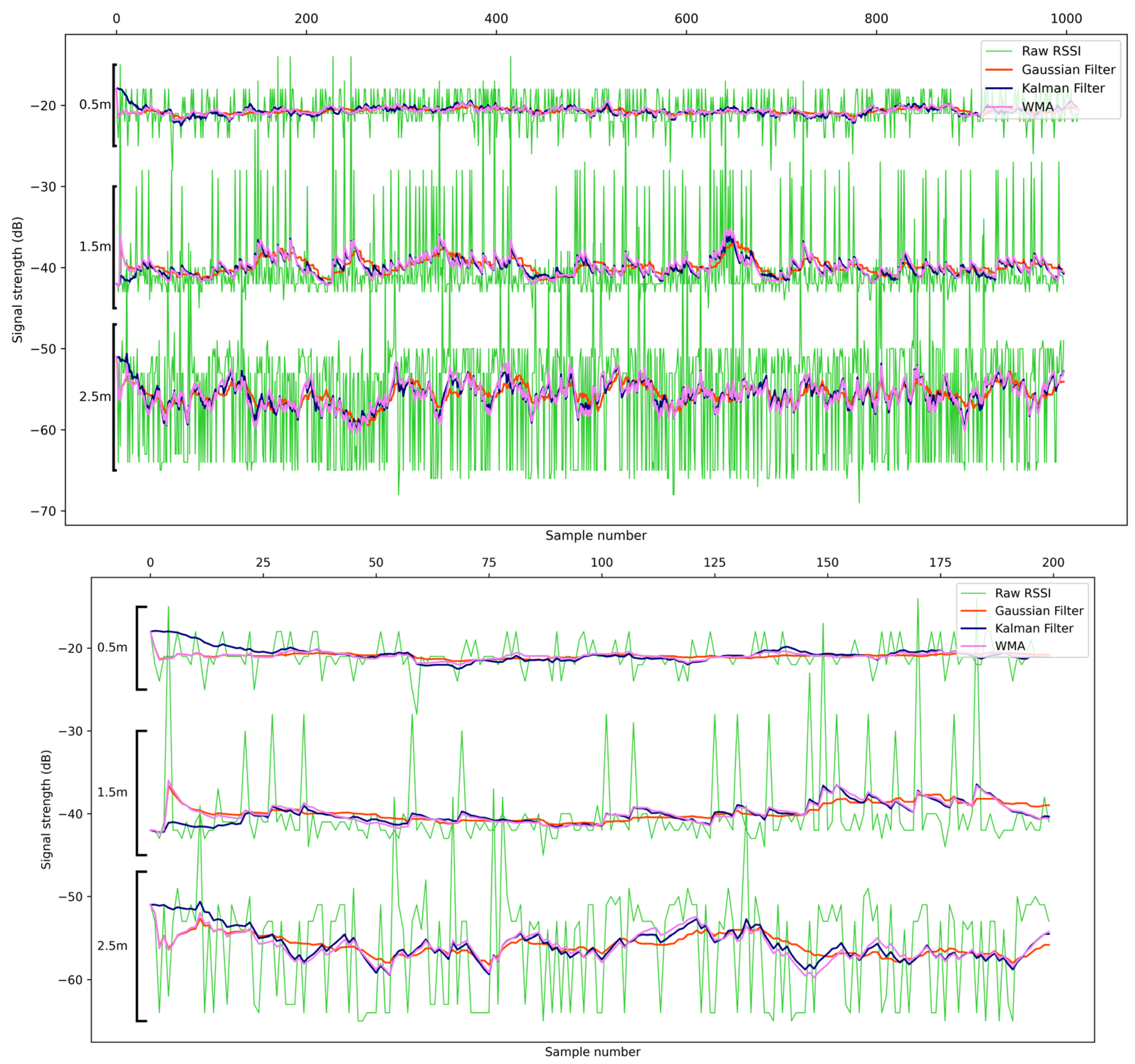
In order to further showcase the reasons that the Gaussian filter is selected, a comparative plot including the row and filtered signals at different distances (0.5, 1.5, and 2.5 m) and the same scenario is presented in Figure 13. We observe that there are some points where a signal has spikes that interfere with another signal and negatively affect its structure. For this reason, we applied filters to normalize the sample to make it more distinct. From the filters applied, we ended up with three that had the best results and are depicted in the middle of each signal: Gaussian (orange), Kalman (blue), and Weighted Moving Average (pink). We observe that the WMA filter responds faster and makes abrupt changes in the signal compared to the Gaussian filter, where the change occurs more smoothly (this is more obvious in the area between 200 and 400 in the X-axis of the sample and at a distance of 1.5 m). On the other hand, the Gaussian manages to make smoother changes when there are fluctuations in the signal, and in this way, we can have a smoother transition (this is observed more at the distance of 2.5 m between 150 and 200 of the X-axis).

6.3. ML Algorithm Results (Distance Estimation)

The same approach as LoS/NLoS classification was followed, using a train/test ratio = 80/20 and random_state = 42, with the main difference that now the problem we must deal with is a regression problem. With this approach, we tested the following algorithms, and the results are shown in

Table 6. Model comparison for LoS/NLoS classification.

Model	MAE (m)	MSE (m2)	RMSE (m)	R2	MAPE (%)	MedAE (m)	Variance
Linear Regression	0.72	0.80	0.89	0.38	45.56%	0.62	0.38
Random Forest Regressor	0.50	0.57	0.76	0.56	30.14%	0.30	0.56
Support Vector Regressor	0.59	0.66	0.81	0.48	33.84%	0.44	0.49
K-Nearest Neighbors Regressor	0.50	0.57	0.76	0.56	30.74%	0.30	0.56
Gradient Boosting Regressor	0.55	0.56	0.75	0.56	34.07%	0.42	0.56

.

Among the models compared, the Random Forest Regressor and the k-nearest neighbors regressor had the best and most consistent performance for all metrics. Both the Random Forest Regressor and the k-nearest neighbors regressor recorded the lowest MAE (0.50), MSE (0.57), and RMSE (0.76) while having a relatively stable R² score of 0.56. While the Gradient Boosting Regressor performed slightly better in terms of MSE (0.56), it was less stable, particularly regarding MAPE (34.07%) and MedAE. Linear Regression performed the worst on all the performance metrics, reflecting its low capacity to represent the nonlinear relationship prevalent in RSSI-based range estimation. Overall, the results validate the suitability of ensemble and non-parametric models (Random Forest and KNN) for representing the complicated, noisy patterns of indoor signal propagation.

6.4. Position Estimation

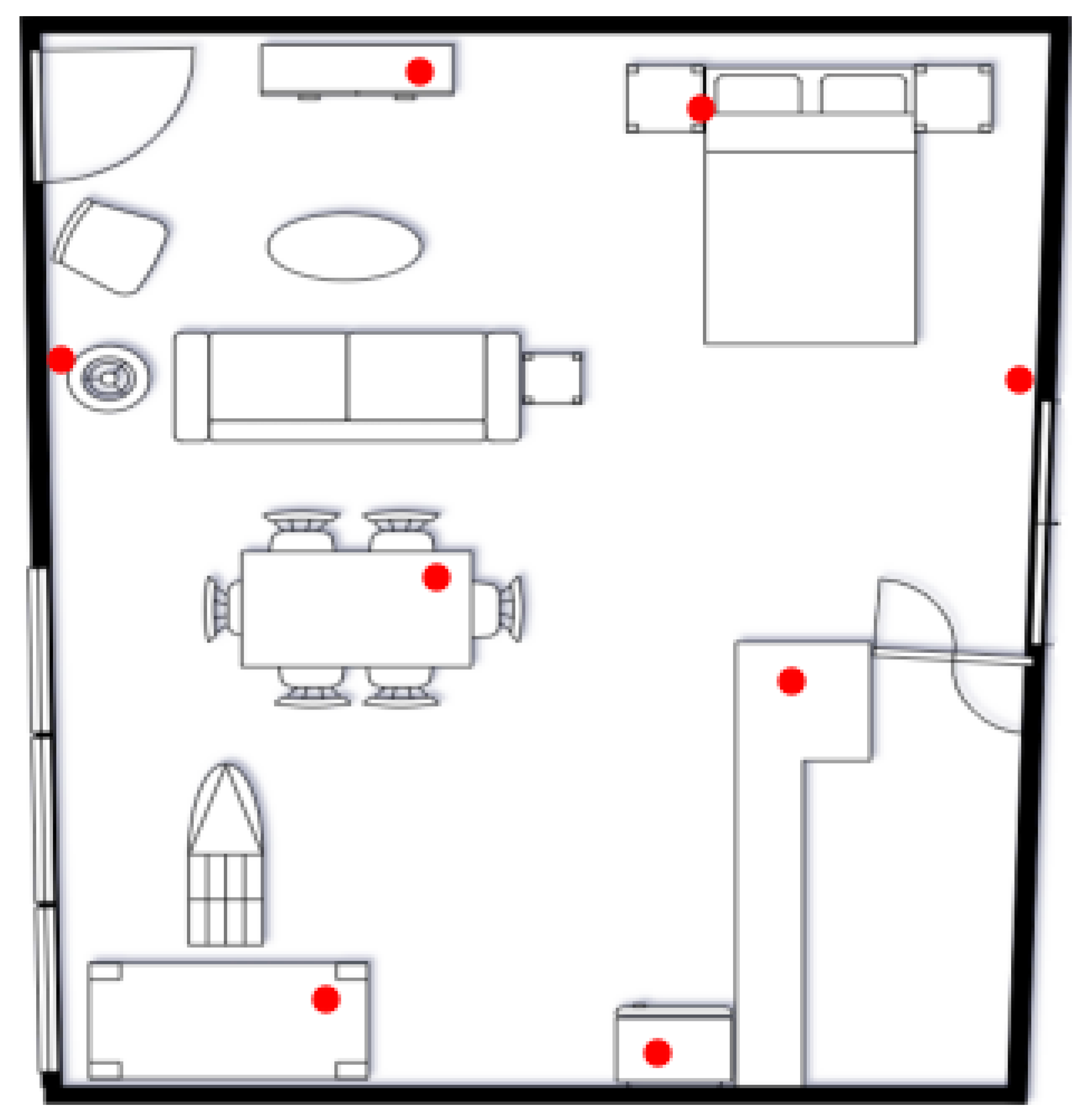
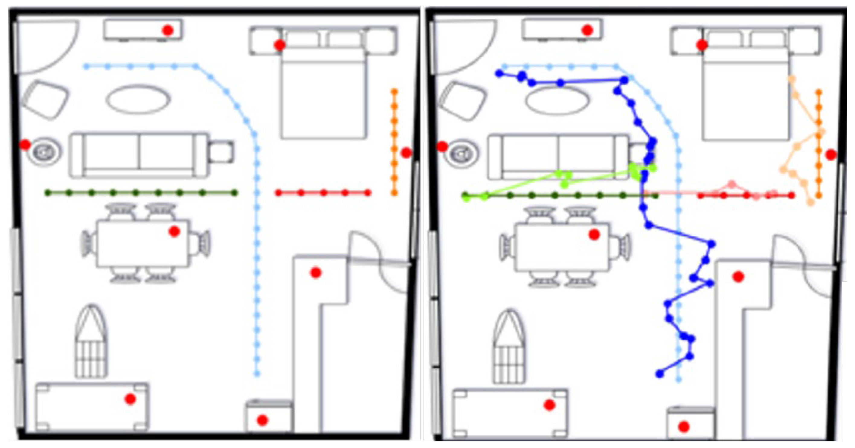
The evaluation of the overall localization system is performed in the surrounding area of AAL House (Figure 11), a controlled indoor environment specifically designed for testing ambient assisting living technologies. Measurements were carried out across four separate paths that cover representative sections of the environment, including corridors, open spaces, and areas with moderate furniture density, as illustrated in Figure 14. Each path was segmented to enable a detailed analysis of system behavior under different spatial configurations. The left part of the figure displays the actual trajectory, whereas the right part provides a visual comparison between the predicted trajectories produced by the proposed localization system and the corresponding ground truth data.

The accuracy of the proposed localization system is assessed using the Root Mean Square Error (RMSE) and the mean localization error as quantitative performance metrics. The results of the localization system estimates are illustrated in

Table 7. Location estimation results.

Route	Mean	STD	CI	RMSE	STD	CI
#1	0.62	0.06	(0.59, 0.65)	0.73	0.09	(0.68, 0.77)
#2	0.51	0.08	(0.47, 0.56)	0.58	0.12	(0.52, 0.64)
#3	0.53	0.16	(0.45, 0.61)	0.60	0.17	(0.51, 0.68)
#4	0.51	0.09	(0.46, 0.56)	0.60	0.12	(0.54, 0.66)

.

To evaluate the performance of the localization system, we conducted 15 independent test rounds across the same set of routes. Among them, Route 1 (blue lines) demonstrated the highest average error (mean error = 0.62 m; RMSE = 0.73 m), yet its relatively narrow confidence intervals indicate consistent, though less accurate, performance. It is noted that this elevated error level observed regarding Route 1, compared to other routes, is likely attributed to a greater number of static and dynamic obstacles present along Route 1, which can cause signal attenuation and multipath effects, reducing the localization accuracy. However, this reduction remains within the acceptable ranges for indoor localization applications. In contrast, Route 2 (red lines) produced the lowest error values (mean error = 0.51 m; RMSE = 0.58 m), coupled with tight confidence bounds—signifying both high accuracy and reliability. This performance can be explained by the absence of significant obstacles along Route 2, allowing for direct line-of-sight communication between the nodes and minimizing signal degradation. Route 3 (green lines) exhibited the widest confidence intervals for both metrics, revealing high variability in system behavior, caused by closely spaced obstacles. Finally, Route 4 (orange Lines) performed comparably to Route 2, with error levels slightly higher but still within a reliable range.

7. ADLS

7.1. ADL Design

Modeling an Activity of Daily Living (ADL) using positional data in an indoor environment involves leveraging spatial context alongside sensor information to infer activities based on a person’s location and movement. Indoor positioning data (from Wi-Fi, Bluetooth, RFID, or other positioning systems) provides information on where the individual is located within a specific area, which can be used to classify activities based on typical spatial patterns associated with each activity.

The first step is to define the ADLs that must be modeled (e.g., eating, cooking, sleeping, walking, or sitting). Each ADL is often linked to a specific location within an indoor environment (

Table 8. ADLs and their location in indoor environments.

Room	ADLs
Kitchen	Cooking, eating, cleaning
Living room	Watching TV, sitting, resting
Bathroom	Showering, washing hands
Bedroom	Sleeping, dressing

).

ADLs are not only location-based but also time-dependent. It is important to recognize that a person might start their activity in one location and move to another (e.g., cooking might start in the kitchen and then transition to sitting at the dining table). To model the temporal context, the time window must be defined, as well as the activity transitions. The next step is to extract features by collecting data from the indoor positioning system as the person moves around the environment. This data might include location coordinates, indicating the person’s position in the room or house; timestamps, to correlate the position with time (e.g., duration in each location); and movement patterns, e.g., movements between rooms or specific locations within a room. The final step is utilizing the positional and temporal features and training a machine learning model to recognize activities based on the person’s location and movement patterns. In this work, three ADLs were defined.

Table 9. ADL descriptions.

ADL	Location	Feature Extraction	Machine Learning
Cooking	Kitchen	Time spent in the kitchen, speed of movement, and transitions between the refrigerator, stove, and sink.	Classify the activity as cooking based on patterns of movement and time spent in the kitchen.
Resting/Sitting	Living Room	Duration of stillness in a specific area, no movement or low movement for an extended period.	Recognize this activity by identifying prolonged stays in the living room with minimal movement.
Sleeping	Bedroom	Long periods of inactivity, detection of the person lying down, and absence of transitions.	Classify the activity as sleeping for long periods in the bedroom with little to no movement.

shows the ADLs, the features related to each one, and the machine learning result.

7.2. Evaluation

The evaluation of the ADLs was carried out by classifying user movement paths between rooms using coordinate data provided in CSV files. Each file represented a single path, containing timestamped coordinates as well as the starting room and ending room. The goal was to build a model that could predict the origin and destination of a path based on its coordinate sequence.

Initially, multiple CSV files were uploaded, each labeled with a specific path such as “office to bed” or “sofa to kitchen.” The coordinate data was parsed from strings like [−6.13, −7.76] and structured into numeric arrays. A preliminary plot was generated where each path was visualized using a line connecting its coordinate points. Figure 15 shows that although the starting and ending areas were relatively distinct, some paths overlapped or intersected, especially around central areas.

A first round of machine learning baselines used summary statistics (mean and deviation) as features and achieved ≤ 40% accuracy across Random Forest, k-nearest neighbors (k-NN), and a multilayer perceptron (MLP). Predictions frequently misidentified paths that overlapped in space, despite having distinct labels.

Flattening coordinate features into fixed-size vectors raised accuracy only marginally. This allowed models to consider more information about each path. Additional features such as path length, direction vectors, and start/end points were also computed and used to refine the model inputs. However, even with these enhancements, accuracy remained low due to the similar shapes among paths.

As a lightweight baseline, a simple rule-based method was implemented. This method stored the start and end coordinates of each known path. When a new path was provided, its start and end coordinates were compared to each known pair using Euclidean distance. The label of the closest known path was returned as the predicted path. This approach assumes that the user’s movement between rooms tends to start and end in consistent physical locations, which was mostly true based on the data. To test the rule-based classifier, six test samples were used (e.g., “office to bed”, “office to kitchen”, etc.). This was further supported by a confusion matrix shown in Figure 16. The rule-based method correctly identified most of them, giving an accuracy of 100%. In two circumstances (bed -> fridge and bed -> kitchen), the model was confused but still made the correct prediction with high accuracy. The confusion derives from the fact that both paths had the same starting point and very close ending points, as shown in Figure 17.

In addition to this, a visualization was created showing only the start and end points of each path. Green dots represented start points, and red dots represented end points. These were connected by dashed lines, and each point was labeled with the associated room. The visualization confirmed that while path shapes overlapped, start and end positions were often distinct enough to uniquely identify the path.

Based on these observations, a hybrid approach was used, combining a rule-based system with a machine learning model to improve path classification accuracy. If a full path has starting and ending coordinates close to a known path, the system confidently assigns the corresponding label using simple distance checks. If the path is ambiguous, the model predicts the most likely destination based on learned patterns. This method balances precision and flexibility, making it ideal for small or overlapping datasets.

In order to have a model with better accuracy without overfitting, data augmentation was performed. The raw dataset consisted of eighteen labeled trajectories—three per ADL class—obtained by interleaving every third sample from each original path. To increase variability, each trajectory was cloned three times using (i) Gaussian jitter (σ = 0.15 m added to every coordinate), (ii) time-warping (stretching the timeline to 120% then resampling back to the original length), and (iii) sequence reversal. This produced 72 sequences (18 original + 54 augmented). The classifier is a Bi-directional LSTM with 64 hidden units, followed by a 30% dropout layer. Weights were learned with Adam (learning rate: 1 × 10⁻³) and early stopping (patience = 5 epochs). To avoid temporal leakage, complete trajectories—not individual samples—were split into 70% train and 30% test. Model selection used a 15% validation slice taken from the training set. Introducing synthetic data augmentation and a sequence-aware classifier raised performance from the ≤40% ceiling of the shallow baselines to 91% accuracy. More details about the Bi-LSTM model architecture are shown in

Table 10. Bi-LSTM model architecture.

Component	Value
Layers	Masking(0.0) → Bi-LSTM(64) → Dropout(0.30) → Dense(C, softmax)
Activations	LSTM internals: tanh/sigmoid; output: softmax
Optimizer	Adam, learning rate 1 ×10−3
Batch size	32
Epochs/early stopping	Max 50; patience 5 on val_loss
Train/val/test split	70/30 by trajectory-group, 20% used as validation
Random seed	42
Metrics (reported on test)	Accuracy, macro-F1, confusion matrix
Evaluation set size	30% of 72 trajectories → 22 trajectories
Protocol used	5-fold cross-validation, grouped by trajectory
Performance variance	Accuracy = 91.0% ± 2.3% (standard deviation across folds)

.

The last challenge was to identify a user’s destination based on their movement path, using coordinate data from CSV files. First, the features from each path were extracted, including coordinates, starting and ending points, and direction. Several machine learning models were trained and combined with a rule-based system to create a hybrid classifier. This hybrid approach uses simple distance checks to confidently match known paths, while relying on the trained model for more ambiguous cases. To handle partial paths, the first half of the file’s coordinates was extracted, and the model predicted where that half-path leads. Even if multiple paths start from the office and end at bed, their paths may differ slightly—especially in the first half.

In

Table 11. Partial predictions.

Bed-to-Kitchen Partial Prediction		Office-to-Bed Partial Prediction
Destination	Probability (%)	Destination	Probability (%)
bed -> kitchen	99.82	office -> bed	75.11
bed -> fridge	0.17	bed -> kitchen	16.45
office -> bed	0.01	armchair -> kitchen	4.28

, two probability tables are shown for the paths from the bed to the kitchen and from the office to the bed. It is clearly shown that the results are better when the path does not overlap with others.

8. Limitations and Future Work

Despite the promising results and the comprehensive design of the proposed localization and ADL monitoring framework, several limitations need to be addressed. One of the primary challenges lies in the sensitivity of RSSI-based positioning to environmental factors such as multipath effects, interference, and dynamic changes in indoor layouts. Although signal filtering and data enrichment processes help mitigate these issues, they cannot fully eliminate the inherent variability of RSSI signals, which may lead to occasional inaccuracies in localization, particularly in cluttered or highly variable environments. One approach to address the variability of RSSI-based positioning involves the adaptation of hybrid approaches that combine multiple techniques, such as sensing modalities (IMUs, etc.) and different localization techniques such as Angle of Arrival (AoA). The approaches can significantly improve robustness by cross-validating positional estimates.

The system also assumes consistent beacon placement and hardware characteristics. In real-world scenarios, hardware variability or battery degradation could affect signal quality, potentially impacting the performance of the machine learning models that were trained under idealized conditions. Similarly, user-specific behavior variations, such as differences in movement patterns or ADL performance, are not currently personalized, which may limit the framework’s accuracy for broader deployment.

Another limitation is the reliance on preconfigured areas of interest and static annotations for ADL detection. While the proposed method is effective for controlled or semi-structured environments, it may struggle to generalize across diverse residential layouts or to adapt to frequent environmental changes without manual intervention. Additionally, the rule-based classifier that was employed in ADL recognition may not scale well for more complex or overlapping paths where behavioral ambiguity increases. Future work will additionally incorporate sensor modalities (e.g., motion or pressure sensors) and explore unsupervised learning techniques to automatically discover activity patterns and spatial structures without requiring labeled data or predefined zones.

The incorporation of data privacy techniques is of paramount importance for localization systems. Collecting sensitive information—such as user presence and behavioral patterns—must be carried out over secure communication channels, ensuring user anonymity throughout the process. To achieve this, data collection and processing are performed at the edge level, with only non-identifiable and uncorrelated data transmitted to cloud servers. This approach significantly reduces security risks while also enhancing the scalability of the system. Furthermore, the localization pipeline is designed to be lightweight, enabling it to run efficiently on edge devices. This allows the system to support multi-user scenarios effectively without compromising performance or privacy.

In terms of future work, one promising direction is the integration of generative adversarial networks (GANs) to synthetically expand RSSI datasets, enhancing the robustness of ML models under varied conditions. Moreover, the feedback loop mechanism, which currently adjusts system parameters post hoc, could be improved with real-time adaptive learning techniques, allowing for dynamic model retraining based on streaming data. Another critical advancement would be the inclusion of context-aware and personalized ADL models that adapt to individual behavior and preferences over time, leveraging sensor measurements.

Finally, with respect to real-world scenarios that can test the limits of the proposed system, we plan to extend the validation to more diverse and large-scale indoor environments. Such evaluations will allow us to assess the system’s robustness under varying conditions, including higher user density, dynamic obstacles, and complex spatial layouts. In doing so, we aim to provide a comprehensive analysis of its scalability and transferability, ensuring that the approach remains effective beyond controlled laboratory settings.

9. Conclusions

This work presents a scalable framework for indoor localization designed to work seamlessly in real-world environments. By using RSSI signal processing, machine learning, and ADL recognition, the system proposed effectively overcomes common challenges such as signal noise and changes in indoor conditions. The integration of machine learning for tasks like distance estimation, LoS/NLoS detection, and activity recognition enables position and ADL monitoring. The experiments conducted showed that each component of the system performs well both separately and combined with the other components. As for future work, the system is planned to be more personalized and adaptable, enhancing safety, independence, and quality of life.