A Novel 3D U-Net–Vision Transformer Hybrid with Multi-Scale Fusion for Precision Multimodal Brain Tumor Segmentation in 3D MRI

Abstract

In recent years, segmentation for medical applications using Magnetic Resonance Imaging (MRI) has received increasing attention. Working in this field has emerged as an ambitious task and a major challenge for researchers; particularly, brain tumor segmentation from MRI is a crucial task for accurate diagnosis, treatment planning, and patient monitoring. With the rapid development of deep learning methods, significant improvements have been made in medical image segmentation. Convolutional Neural Networks (CNNs), such as U-Net, have shown excellent performance in capturing local spatial features. However, these models cannot explicitly capture long-range dependencies. Therefore, Vision Transformers have emerged as an alternative segmentation method recently, as they can exploit long-range correlations through the self-attention mechanism (MSA). Despite their effectiveness, ViTs require large annotated datasets and may compromise fine-grained spatial details. To address these problems, we propose a novel hybrid approach for brain tumor segmentation that combines a 3D U-Net with a 3D Vision Transformer (ViT3D), aiming to jointly exploit local feature extraction and global context modeling. Additionally, we developed an effective fusion method that uses upsampling and convolutional refinement to improve multi-scale feature integration. Unlike traditional fusion approaches, our method explicitly refines spatial details while maintaining global dependencies, improving the quality of tumor border delineation. We evaluated our approach on the BraTS 2020 dataset, achieving a global accuracy score of 99.56%, an average Dice similarity coefficient (DSC) of 77.43% (corresponding to the mean across the three tumor subregions), with individual Dice scores of 84.35% for WT, 80.97% for TC, and 66.97% for ET, and an average Intersection over Union (IoU) of 71.69%. These extensive experimental results demonstrate that our model not only localizes tumors with high accuracy and robustness but also outperforms a selection of current state-of-the-art methods, including U-Net, SwinUnet, M-Unet, and others.

1. Introduction

Nowadays, the rapid advances in deep learning are revolutionizing the field of medical image analysis by providing more accurate and efficient diagnostic tools [1,2]. Work in this field is both ambitious and challenging, and tumor segmentation in medical images is a critical task [3]. In particular, brain tumors are among the most common and deadliest diseases of the central nervous system (CNS) [4]. Therefore, understanding brain tumors and their various types is important for addressing their impact on brain health and patient survival. Brain tumors consist of abnormal cell growths occurring in or near the brain, and they typically include meningiomas, gliomas, and pituitary tumors. Gliomas are considered to be the most prevalent and aggressive type of brain tumor. There are two types of gliomas: low-grade gliomas (LGG) and high-grade gliomas (HGG), with the latter being more aggressive and associated with poorer survival rates, often requiring surgery and radiotherapy [5]. Even after treatment, median overall survival for patients with HGG is often no more than 14 months [4]. Because brain tumors, especially high-grade gliomas, are highly aggressive, accurate and timely diagnosis is essential for improved patient outcomes. Magnetic Resonance Imaging (MRI) has emerged as one of the most widely used clinical imaging modalities for diagnosing and treating brain tumors [6], given its ability to produce high-quality, non-invasive brain images. However, manual segmentation of brain tumors from MRI scans by radiologists and other experts is time-consuming, labor-intensive, and prone to error [7].

Therefore, automatic brain tumor segmentation methods based on deep learning have gained increasing attention recently, owing to their potential to improve accuracy, consistency, and efficiency. Among deep learning models, U-Net has emerged as the most popular architecture for medical image segmentation [8], with its encoder–decoder structure and skip connections that help preserve spatial details. This architecture has achieved significant success in numerous medical segmentation tasks, such as organ, heart, and lesion segmentation [9,10,11]. Despite its strengths in medical image processing, U-Net’s convolutional operations have intrinsic limitations in capturing long-range dependencies. Recent studies have shown that convolution-based models like U-Net struggle to capture long-range dependencies effectively, which can limit their performance in complex medical segmentation tasks [12,13]. To address these limitations, Vision Transformers (ViTs) have been introduced to medical imaging tasks for their ability to model global contextual information via self-attention mechanisms [14]. Self-attention is the core component of the transformer encoder. However, ViTs typically require large annotated datasets for effective training, and their performance may be limited when only small medical datasets are available [15,16]. Compared to U-Net and traditional CNN models, ViTs are inherently more capable of learning global representations, which is especially beneficial in complex segmentation scenarios such as brain tumor segmentation. However, ViTs typically require large quantities of annotated data for effective training and may lose fine-grained spatial information throughout the tokenization and path embedding operations [17].

To leverage the strengths of both architectures, recent research has focused on hybrid models that combine the local feature-extraction capability of U-Net with the global reasoning power of Vision Transformers. In this work, a novel hybrid approach is proposed, combining a 3D U-Net and a 3D Vision Transformer (ViT3D) to address the MRI brain tumor segmentation task. These contributions distinguish our proposed hybrid model from existing U-Net/ViT approaches by integrating unique design elements that enhance both local feature extraction and global context modeling.

To sum up, the main contributions of this paper are summarized as follows:

• The integration of a 3D U Net encoder–decoder with a native 3D Vision Transformer, which enables the model to capture fine-grained anatomical details via skip connections while simultaneously modeling long-range spatial dependencies through multi-head self-attention.
• The design of a flexible patch-based pipeline supporting optional overlap and lightweight 3D augmentations, whereby increased sample diversity through overlapping patches and random flips along all axes enhances generalization on limited medical datasets.
• The application of training strategies to improve efficiency and convergence.
• The proposal of a multimodal architecture that exploits MRI inputs (T1, T1-CE, T2, and FLAIR) through early stacking of volumes, combined with inter-modal attention in the Vision Transformer branch, allows the network to leverage complementary contrast information for more precise tumor boundary delineation and edema detection.

The rest of the paper is organized as follows: Section 2 outlines the related work. Section 3 presents the structure of our novel approach. Section 4 describes the dataset and experimental setup. Section 5 provides results and analysis, including discussions and comparisons with existing methods. Finally, we conclude in Section 6.

2. Related Work

In this section, we review recent research on brain tumor segmentation and the strategies proposed to address the limitations of U-Net and Vision transformers. Then, a summary of these approaches is presented in Table 1.

2.1. U-Net-Based Models

The study introduced by Chen et al. [18] proposed the MAU-Net method for MRI brain tumor segmentation, which integrates mixed-depthwise convolution (MDConv) [19] in the encoder and decoder to capture multi-scale features, a context pyramid module (CPM) [20] in the skip connections to strengthen semantic context, and a self-ensemble module [21] to improve segmentation accuracy.

In their study, Abousaleh et al. [22] developed VGG-19+Decoder, a hybrid model combining U-Net with a VGG-19 backbone for brain tumor segmentation in MRI. The VGG-19 backbone extracts robust features from the images, while the decoder reconstructs the segmentation mask to delineate tumor boundaries. This approach simplifies U-Net while leveraging VGG-19’s feature extraction, achieving high segmentation accuracy (96.1%) and strong generalization (CCR 95.69%) without requiring GPU acceleration.

In addition, Rehman et al. [23] presented Bu-Net, a U-Net-based hybrid model for MRI brain tumor segmentation. It incorporates a Residual Extended Skip (RES) block to preserve multi-scale features and a Wide Context (WC) block to enhance spatial context, improving segmentation accuracy for tumor regions. Evaluated on BraTS 2017 [24] and 2018 datasets [25], Bu-Net outperformed the standard U-Net, particularly for tumor core (TC), whole tumor (WT), and enhancing core (EC) regions. Also, Sourodip et al. [26] proposed a U-Net with a VGG-16 backbone for brain tumor segmentation in MRI images. The VGG-16 encoder extracts robust features, while the U-Net decoder reconstructs the segmentation mask, leading to improved accuracy. Evaluated on the TCGA-LGG dataset [27] using K-fold cross-validation, the model achieved a pixel accuracy of 0.9975, outperforming standard U-Net and other CNN-based methods.

Moreover, Nizamani et al. [28] introduced FE-HU-NET, a hybrid U-Net model for brain tumor segmentation in MRI. The proposed model combines preprocessing to enhance image quality, a customized U-Net (HU-Net) for feature extraction, and CNN-based post-processing to refine segmentation boundaries. Tested on BraTS and LGG-MRI-Segmentation datasets, FE-HU-NET achieved 99% accuracy, outperforming state-of-the-art methods on key metrics such as the Jaccard index, sensitivity, and specificity.

In order to overcome the limits of the inadequacy of single-modality imaging, Zhao et al. [29] proposed M-UNet, a hybrid U-Net model for multimodal MRI brain tumor segmentation. The model uses multiple encoders to extract features from different modalities, a single decoder to reconstruct the segmentation mask, a hybrid attention block (HAB) for feature enhancement, and a dilated convolution block (DCB) for multi-scale feature capture. The experimental results on the BraTS 2020 dataset demonstrated that M-UNet achieved an average Dice score of 79.2% and a Hausdorff distance of 8.466, outperforming standard U-Net [30], Attention U-Net [31], and ResUNet + + [32].

Lastly, in their study, Butt et al. [33] presented a Hybrid Multihead Attentive U-Net for MRI brain tumor segmentation. The model incorporates multihead attention to focus on informative regions and improve boundary detection. Tested on the BraTS 2020 benchmark dataset and compared with existing architectures known as SegNet [34], FCN-8s [35], and Dense121 U-Net [36]. The result indicates that the proposed architecture outperforms the compared benchmarks across key performance metrics.

2.2. Vision Transformer-Based Models

Vision Transformer (ViT) models have been applied to brain tumor segmentation to improve accuracy and mitigate data imbalance. Numerous ViT-based methods have been extensively studied and have demonstrated strong performance on brain tumor segmentation tasks. The first study cited in this subsection concerns Wang et al. [37]. The authors proposed TansBTS, a hybrid 3D CNN–Transformer model for multimodal MRI brain tumor segmentation. The 3D CNN encoder captures local spatial features, while the Transformer module models long-range global context. The decoder integrates these features and applies progressive upsampling to produce accurate segmentation maps. The framework was validated on both the BraTs2019 and BraTs2020 datasets, and the results show that TansBTS demonstrated performance on par with or superior to state-of-the-art 3D segmentation models. The second study worth mentioning is the work of Hatamizadeh et al. [38], who developed UNETR, a transformer-based U-Net model for volumetric medical image segmentation. The Transformer encoder captures global contextual information across multiple scales, while the U-shaped decoder reconstructs the segmentation mask via skip connections. Evaluated on BTCV [39] and MSD datasets [40]. In these evaluations, UNETR achieved state-of-the-art performance, demonstrating its effectiveness at modeling intricate anatomical features and opening new possibilities for future transformer-based models in medical image analysis.

Also, Liu et al. [41] proposed BRAINNET, a hybrid segmentation pipeline for glioblastoma using an ensemble of MaskFormer-based Vision Transformers. Each model is fine-tuned along axial, sagittal, and coronal planes, and the ensemble combines predictions to produce precise segmentation masks for tumor subregions. The model was trained and tested on the UPenn-GBM dataset and achieved state-of-the-art results with high Dice coefficients and low Hausdorff distances for tumor core, whole tumor, and enhancing tumor.

Similarly, the scholarly paper by Nian et al. [42] introduced 3D BrainFormer, a transformer-based framework for brain tumor segmentation directly on 3D MRI volumes. The model incorporates novel attention mechanisms, including Fusion Head Self-Attention (FHSA) and the Infinite Deformable Fusion Transformer Module (IDFM), to enhance multi-scale feature extraction and capture complex tumor structures. Experimental evaluations on the public BraTS datasets highlight that this architecture outperforms state-of-the-art approaches across multiple metrics: Dice, sensitivity, PPV, and Hausdorff distance. Furthermore, Zhou et al. [43] introduced nnFormer, a 3D Transformer architecture for volumetric medical image segmentation. The model combines local and global volume-based self-attention and replaces standard skip connections with a skip-attention mechanism to enhance feature fusion. Validated on three public datasets, nnFormer outperformed state-of-the-art models, including nnU-Net, in terms of Dice Similarity Coefficient and Hausdorff Distance.

In their recent work, Perera et al. [44] introduced SegFormer3D, a hierarchical Transformer for volumetric medical image segmentation. The model employs multiscale hierarchical attention with a lightweight MLP decoder, enabling efficient feature extraction with significantly reduced computational cost. Tested on the Synaps, BraTs, and ACDC datasets, it gives comparable results with 13 times less processing and 33 times fewer parameters than existing models such as UNETR [37] and nnFormer [43], highlighting its potential as an efficient yet powerful solution.

In addition, Liu et al. [45] developed the 3D Medical Axial Transformer (3D MAT), an efficient architecture for volumetric brain tumor segmentation. Unlike 2D slice-based transformers, 3D MAT leverages axial attention to capture semantic information across the depth dimension while reducing computational costs. To address limited medical datasets, a self-distillation strategy was integrated. Tested on the BraTS 2018 dataset, the model achieved sharper segmentation boundaries and outperformed prior methods while maintaining a lightweight design suitable for clinical use.

In the last two examples, Hu Cao et al. [46] have introduced Swin-Unet, a pure transformer-based U-shaped encoder–decoder architecture tailored for medical image segmentation. The model leverages Swin Transformer blocks as its core units to capture long-range semantic dependencies. Validated on multi-organ and cardiac segmentation tasks, Swin-Unet demonstrated excellent performance and strong generalization, surpassing both convolution-based and hybrid models. Chen et al. [47] proposed TransUNet, a hybrid model that combines the strengths of Transformers and the U-Net architecture for medical image segmentation. The Transformer captures global context by encoding image patches, while the U-shaped design recovers fine-grained details by leveraging local CNN features. This model has been shown to outperform several existing methods, including CNN-based self-attention approaches, on tasks such as multi-organ and cardiac segmentation, highlighting the effectiveness of combining Transformers with U-Net for accurate segmentation.

Table 1. Summary of hybrid U-Net- and Transformer-based models for medical image segmentation.

Model	Key Features	Advantages	Inconvenient
MAU-Net [18]	MDCon, Context Pyramid Module (CPM)	- Better multi-scale feature and spatial context - Precise segmentation	- Increased complexity and computation
VGG-19 + Decoder [22]	U-Net—VGG-19 backbone	- High accuracy and generalization - Efficient on CPU	- No GPU accelerator tested
Bu-Net [23]	RES block, WC block	- Better multi-scale and context capture - Improved segmentation	- Slightly more complex than standard U-Net
U-Net + VGG-16 [26]	VGG-16 backbone	- High segmentation accuracy	- Slightly more complex than standard U-Net
FE-HU-Net [28]	Preprocessing, HU-Net, CNN, Post-processing	- Very high accuracy - Improved boundary refinement	- More complex pipeline - Multiple variants
M-Unet [29]	Multi-encoder Single decoder, HAB, DCB	- Multimodal feature fusion - Improved multi-scale segmentation	- More dice score compared to some latest models
Hybrid Multihead Attentive U Net [33]	Multihead attention	- Improved boundary detection - Better focus on informative regions	- More complex than standard U-Net
TransBTS [37]	3DCNN encoder, Transformer progressive decoder	- Capture local and global features - Accurate 3D segmentation	- More complex architecture - Higher computational cost
UNETR [38]	Transformer encoder U-shaped decoder with skip connections	- Capture global context - Effective for volumetric segmentation	- High computational cost - Complex architecture
BRAINET [41]	Ensemble of mask former-based ViTs, multi-plane prediction	- Accurate segmentation of tumor subregions	- High computational cost
3D Brain-Former [42]	FHSA for multi-scale attention fusion. IDFM for deformable feature extraction	- Outperforms SOTA across Dice, Sensitivity, PPV, HD95	- Complex design - Computationally expensive
nnFormer [43]	Local and global self-attention Skip attention instead of standard skip connections	- Superior Dice and HD95	- High computational complexity
SegFormer3D [44]	Hierarchical multiscale attention Lightweight MLP encoder	- Competitive performance	- May sacrifice some accuracy compared to heavier models
3D MAT [45]	Axial attention + self-distillation	- Compact and suitable for clinical use	- Limited evaluation
Swin-Unet [46]	Swin Transformer blocks	- Strong generation - Outperforms CNN and hybrid models	- Computation demand
TransUNet [47]	Transformer encoder for global context CNN decoder for global detail	- Outperforms CNN, Self-attention models - Accurate segmentation	- Still computationally heavy

Table 1. Summary of hybrid U-Net- and Transformer-based models for medical image segmentation.

Model	Key Features	Advantages	Inconvenient
MAU-Net [18]	MDCon, Context Pyramid Module (CPM)	- Better multi-scale feature and spatial context - Precise segmentation	- Increased complexity and computation
VGG-19 + Decoder [22]	U-Net—VGG-19 backbone	- High accuracy and generalization - Efficient on CPU	- No GPU accelerator tested
Bu-Net [23]	RES block, WC block	- Better multi-scale and context capture - Improved segmentation	- Slightly more complex than standard U-Net
U-Net + VGG-16 [26]	VGG-16 backbone	- High segmentation accuracy	- Slightly more complex than standard U-Net
FE-HU-Net [28]	Preprocessing, HU-Net, CNN, Post-processing	- Very high accuracy - Improved boundary refinement	- More complex pipeline - Multiple variants
M-Unet [29]	Multi-encoder Single decoder, HAB, DCB	- Multimodal feature fusion - Improved multi-scale segmentation	- More dice score compared to some latest models
Hybrid Multihead Attentive U Net [33]	Multihead attention	- Improved boundary detection - Better focus on informative regions	- More complex than standard U-Net
TransBTS [37]	3DCNN encoder, Transformer progressive decoder	- Capture local and global features - Accurate 3D segmentation	- More complex architecture - Higher computational cost
UNETR [38]	Transformer encoder U-shaped decoder with skip connections	- Capture global context - Effective for volumetric segmentation	- High computational cost - Complex architecture
BRAINET [41]	Ensemble of mask former-based ViTs, multi-plane prediction	- Accurate segmentation of tumor subregions	- High computational cost
3D Brain-Former [42]	FHSA for multi-scale attention fusion. IDFM for deformable feature extraction	- Outperforms SOTA across Dice, Sensitivity, PPV, HD95	- Complex design - Computationally expensive
nnFormer [43]	Local and global self-attention Skip attention instead of standard skip connections	- Superior Dice and HD95	- High computational complexity
SegFormer3D [44]	Hierarchical multiscale attention Lightweight MLP encoder	- Competitive performance	- May sacrifice some accuracy compared to heavier models
3D MAT [45]	Axial attention + self-distillation	- Compact and suitable for clinical use	- Limited evaluation
Swin-Unet [46]	Swin Transformer blocks	- Strong generation - Outperforms CNN and hybrid models	- Computation demand
TransUNet [47]	Transformer encoder for global context CNN decoder for global detail	- Outperforms CNN, Self-attention models - Accurate segmentation	- Still computationally heavy

3. Proposed Model

3.1. Architecture Overview

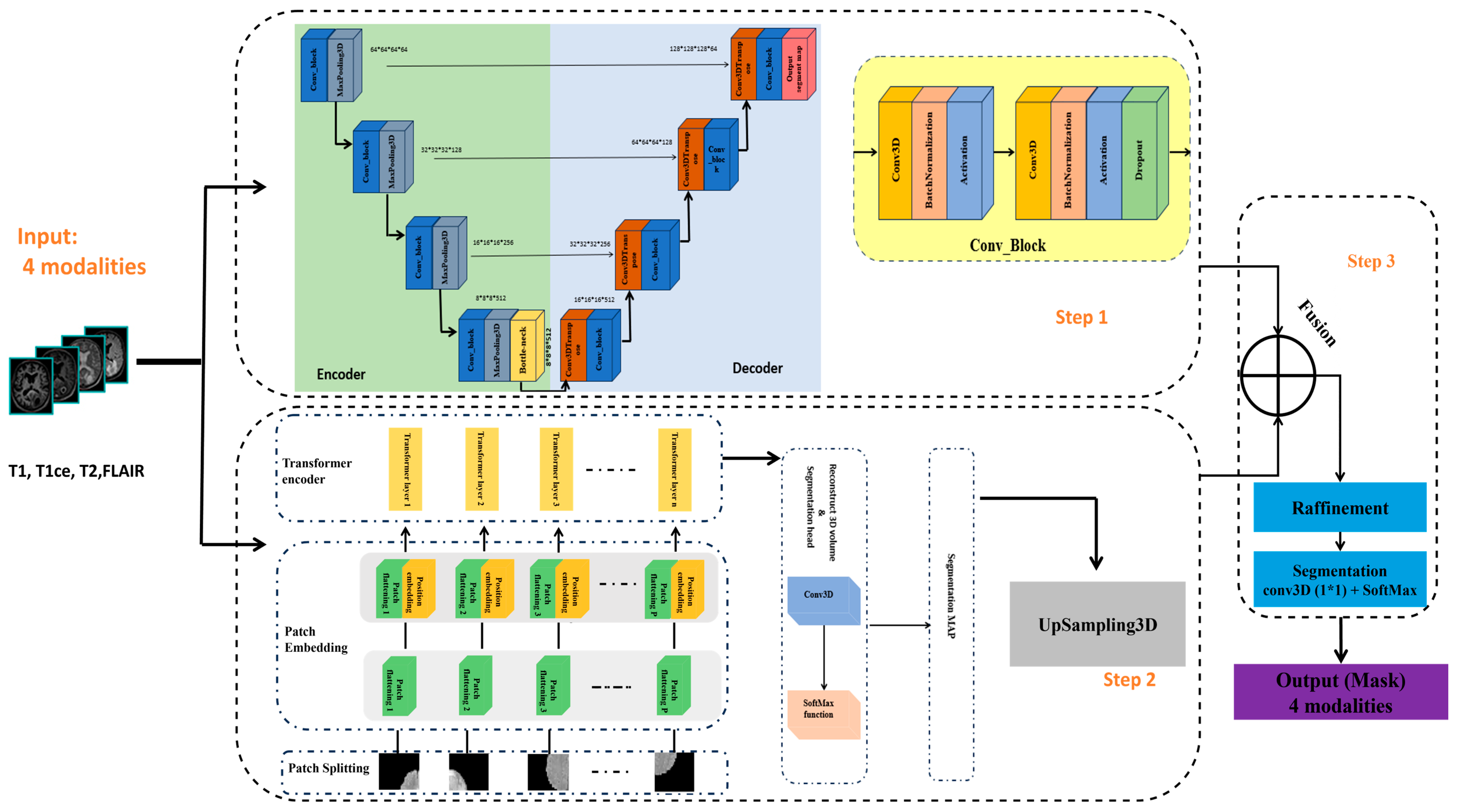
In this study, we propose a 3D brain tumor segmentation architecture that combines a 3D Vision Transformer (ViT) with a 3D U-Net model, as illustrated in Figure 1. The overall architecture of our proposed model is composed of three main components. First, a 3D U-Net encoder–decoder structure is used to extract local features and preserve anatomical details using hierarchical convolutional layers. In parallel, a 3D Vision Transformer component processes the same input volume by partitioning it into 3D patches and employing self-attention mechanisms to capture long-range relationships and global context within the data. Finally, the outputs from both components are fused after aligning their spatial resolutions and are refined using convolutional and normalization layers to improve prediction accuracy. This hybrid approach effectively combines local detail and global context, enhancing the model’s ability to segment complex tumor subregions.

Figure 1. Schematic diagram of the proposed model for brain tumor segmentation.

The model receives 3D MRI volumes of size 128 × 128 × 128 with four channels, each corresponding to a different imaging modality (T1, T1ce, T2, and FLAIR), as provided by the BraTS 2020 v1.2.1 dataset.

In the following, we describe the components of our approach in detail.

3.1.1. Step 1: 3D U-Net Component

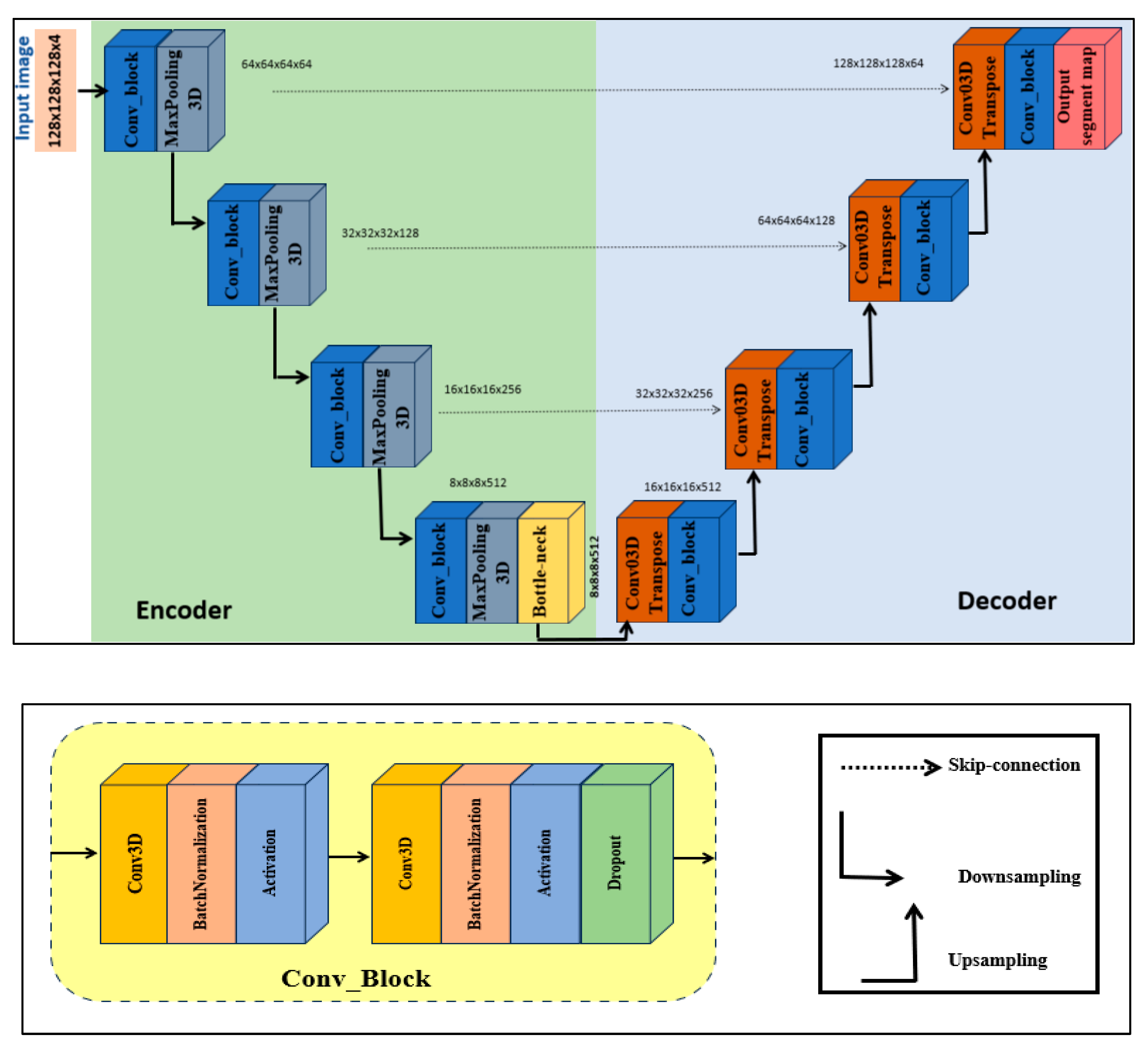
U-Net was introduced by Ronneberger et al. [26] in 2015. It has gained widespread adoption in medical image segmentation tasks, particularly in brain tumor segmentation. Inspired by the U-Net structure and its ability to capture rich local features and maintain spatial details through skip connections, we were motivated to adopt a 3D extension of the U-Net as one of the core components of our proposed model. To facilitate the understanding of the 3D U-Net block within our model, the network structure table is given in Table 2. Figure 2 illustrates the specific architecture of the 3D U-Net. The design consists of three parts, namely the encoder, bottleneck, and decoder.

Table 2. Three-dimensional U-Net network structure table.

Stage	Encoder	Output Size	Decoder	Output Size
0	Input	128 × 128 × 128 × 4	Conv3D [output Layer] [1 × 1]	128 × 128 × 128 × 4
1	(Conv3D [3 × 3 × 3, BatchNorm, Relu] Dropout [dropout_rate = 0.1]) × 2 MaxPooling3D [2 × 2 × 2]	64 × 64 × 64 × 64	Conv3DTranspose [64] (Conv3D [3 × 3 × 3, BatchNorm, Relu] Dropout [ dropout_rate = 0.1]) × 2	128 × 128 × 128 × 64
2	(Conv3D [3 × 3 × 3, BatchNorm, Relu] Dropout [dropout_rate = 0.1]) × 2 MaxPooling3D [2 × 2 × 2]	32 × 32 × 32 × 128	Conv3DTranspose [128] (Conv3D [3 × 3 × 3, BatchNorm, Relu] Dropout [ dropout_rate = 0.1]) × 2	64 × 64 × 64 × 128
3	(Conv3D [3 × 3 × 3, BatchNorm, Relu] Dropout [dropout_rate = 0.1]) × 2 MaxPooling3D [2 × 2 × 2]	16 × 16 × 16 × 256	Conv3DTranspose [256] (Conv3D [3 × 3 × 3, BatchNorm, Relu] Dropout [ dropout_rate = 0.1]) × 2	32 × 32 × 32 × 256
4	(Conv3D [3 × 3 × 3, BatchNorm, Relu] Dropout [ dropout_rate = 0.1]) × 2 MaxPooling3D [2 × 2 × 2]	8 × 8 × 8 × 512	Conv3DTranspose [512] (Conv3D [3 × 3 × 3, BatchNorm, Relu] Dropout [ dropout_rate = 0.1]) × 2	16 × 16 × 16 × 512
5	(Conv3D [3 × 3 × 3, BatchNorm, Relu] Dropout [ dropout_rate = 0.1]) × 2	8 × 8 × 8 × 1024	_	_

Figure 2. Three-dimensional U-Net block.

• Encoder. The input volume has dimensions 128 × 128 × 128 and is initially fed into the encoder. The encoder systematically reduces spatial resolution using a series of specialized blocks while preserving spatial features. Each block contains two 3D convolutional layers. To achieve stable and robust learning, batch normalization and a ReLU activation function are applied, together with a dropout rate of 0.1 to prevent overfitting. The number of filters doubles at each level, increasing from 64 to 128, then to 256, and finally to 512. After each level, a 3D max-pooling operation with stride 2 reduces spatial dimensions while retaining semantic information (downsampling).
• Bottleneck. The bottleneck, situated between the encoder and decoder, uses 1024 filters to capture the most abstract and high-level features from the input.
• Decoder. The decoder mirrors the encoder. Each upsampling stage employs a 3D transposed convolution layer with stride 2, followed by two 3D convolutional layers with batch normalization and ReLU activations. After each upsampling operation, the decoder concatenates detailed features from the corresponding encoder stage via skip connections.

Finally, the output layer is a 3D convolutional layer with kernel size 1 and softmax activation function. The output of the 3D U-Net is concatenated with the output of the 3D ViT block to produce the final volumetric segmentation.

3.1.2. Step 2: 3D ViT Component

In this section, we present a detailed overview of the 3D ViT component of our model as summarized in Table 3. The Vision Transformer 3D (ViT3D) module is designed to capture global contextual information from volumetric data by leveraging the self-attention mechanism of transformers. Given its efficiency and strong performance in capturing global features, we include this module in our proposed architecture. It works in parallel with the 3D U-Net. The 3D ViT block, as shown in Figure 3, mainly consists of three steps: patch embedding, transformer encoder, and segmentation head.

Table 3. Details of setting layers in the 3D ViT block.

Stage	Operation	Output Size
1	Input (4 channels (T1, T1ce, T2, FLAIR))	128 × 128 × 128 × 4
	Patch Splitting and embedding	16 × 16 × 16 × 128 → 4096 tokens of size 128
	Conv3D [filters = 128, kernel = 8, strides = 8]
	Flatten to tokens: reshape (batch, 4096, 128)
2	Add positional embedding Learnable pos_emb of shape (1, 4096, 128) added to each token	(batch, 4096, 128)
3	Bloc Transformer encoder (∗4)	(batch, 4096, 128)
	LayerNormalization []
	MultiHeadAttention []
	Dropout [dropout_rate = 0.1]
	Residual connections
	LayerNormalization []
	FFN [Dense 512 → Dropout → Dense 128 → Dropout]
	Residual connections
4	Reconstruct 3D volume                          Reshape tokens back: reshape (batch, 16, 16, 16, 128)	16 × 16 × 16 × 128
5	Segmentation head                       Conv3D (filters = 4, kernel_size = 1, activation = ‘softmax’)	16 × 16 × 16 × 4

Figure 3. Three-dimensional ViT block.

Patch embedding. Given an input 3D MRI volume from the BraTS2020 dataset, denoted as $X \in {IR}^{D\times H\times W\times C}$ with the spatial resolution H×W, depth D, and C channels (modalities), we first partition the 3D volume into non-overlapping patches using a 3D convolutional layer with kernel size and stride equal to the patch size P. This process converts each patch into a fixed-dimensional embedding vector, which effectively captures both spatial and depth information. The output tensor $F \in {IR}^{D^{\prime }\times H^{\prime }\times W^{\prime }\times d}$ with $D^{\prime } = D/P$, $H^{\prime } = H/P$ and $W^{\prime } = W/P$ is then reshaped into a sequence of tokens, where each token represents a patch, as presented in Equation (1).

$$f=reshape(F)\in {IR}^{\mathit{N}\times \mathit{d}} \mathrm{with} N=D^{\prime }.H^{\prime }.W^{\prime }$$

(1)

After that, a trainable Positional Embedding (PE) is added to the feature map f to restore spatial relationships lost during the flattening process and is computed as shown in Equation (2).

$$Z=f+PE$$

(2)

Finally, the resulting sequence of tokens Z, enriched with positional information, is fed into the Transformer encoder block to model long-range dependencies across the entire volumetric space.

Transformer encoder. This block is composed of L layers, each of which has two main components: the Multi-Head Attention mechanism (MHA) and a Feed-Forward Network (FFN). To obtain the output of the transformer’s Lth layer, use the following calculations in Equations (3) and (4):

$$Z^{\mathit{l}}=\mathrm{M}\mathrm{H}\mathrm{A}(\mathrm{L}\mathrm{N}(Z^{\{\mathit{l}-1\}}))+Z^{\{\mathit{l}-1\}}$$

(3)

$$Z^{\mathit{l}}=\mathrm{F}\mathrm{F}\mathrm{N}(\mathrm{L}\mathrm{N}(Z^{\mathrm{l}})+Z^{\mathrm{l}}$$

(4)

where LN(·) denotes the layer normalization operator and $Z^{\mathit{l}}$ is the output of the Lth transformer layer. In practice, each block begins with a layer normalization, then applies an MHA to capture diverse relationships in the data, and is followed by a dropout layer to reduce overfitting. A second layer normalization prepares the output for the FFN module, which consists of a two-layer multi-layer perceptron (MLP) with the GELU activation function and an intermediate expansion factor of four, with dropout applied between layers.

Segmentation head. At the end of the network stage, a pointwise $(1\times 1\times 1)$ 3D convolution layer is applied, which converts the deep 3D feature map into a prediction for each voxel, indicating its class. Then, a softmax activation is used to convert these outputs into probabilities for each voxel, ensuring that each voxel is assigned to exactly one class. Finally, a UpSampling3D layer is applied to upsample the ViT3D output to match the spatial dimensions of the final decoder output.

3.1.3. Step 3: Feature Fusion and Segmentation Output

In the last stage of our hybrid model, the decoder output from the 3D U-Net (Step 1) is combined with the upsampled output from the 3D ViT (Step 2) along the channel dimension, immediately after the final decoder layer of the 3D U-Net, effectively integrating local structural features extracted by the convolutional U-Net with global contextual features captured by the transformer-based ViT pathway.

To ensure proper spatial alignment, the ViT output is upsampled using 3D upsampling in the segmentation head before concatenation. This concatenation enables the model to integrate local and global features effectively. Specifically, the subsequent 3D convolutional layers, followed by normalization and activation functions, refine the concatenated features by integrating local and global information, effectively reducing redundancy and harmonizing feature scales. The fused feature volume is then passed through a sequence of 3D convolutional layers, each followed by normalization and activation functions to enhance the combined representation. These methods help enhance feature interactions and mitigate any redundancy or scale mismatch introduced during the fusion process.

Finally, to generate the final segmentation output, we employ a 3D convolutional layer with a $1\times 1\times 1$ kernel followed by a softmax activation function. This crucial last step assigns a class label to each voxel. This results in precise instance segmentation masks that reflect both detailed spatial boundaries and broader anatomical context.

4. Experiments

4.1. Implementation Details

The proposed model was conducted on the Kaggle platform using a GPU accelerator (NVIDIA Tesla T4, 16 GB) of the NVIDIA Corporation manufactured in Taiwan. It was implemented with the TensorFlow deep learning framework and the functional Keras API to ensure flexible and easy development. The Nibabel v5.3.0 library was also used in the preprocessing pipeline, particularly for handling medical image input and output in the NIfTI format for MRI data. These tool choices were made to facilitate simplicity of implementation, promote reproducibility, and support a smooth learning curve for engineers or clinicians aiming to adapt or deploy the method. The model was trained for 50 epochs using the Adam optimizer applied to both the U-Net and ViT branches. We tested up to 200 epochs and observed that after 50 epochs, improvements in validation performance (Dice score and accuracy) became marginal, while additional epochs increased training time without significant gains. An early stopping criterion was applied to prevent overfitting. The same categorical cross-entropy loss, described in Section 4.5, was applied to the outputs of both the U-Net and ViT branches to ensure consistent supervision across the hybrid model. A batch size of four and an appropriate learning rate were used to avoid out-of-memory (OOM) issues. Early stopping and learning rate scheduling help the network converge efficiently and achieve the training objectives.

4.2. Dataset Description

In our study, we conducted experiments on the publicly available BraTS 2020 benchmark dataset v.1.2.1 to verify the effectiveness of the proposed model. BraTS 2020 comprises an annotated training set with 369 patients and a validation set of 125 patients. It includes multimodal scans of 293 high-grade gliomas and 79 low-grade gliomas. For each patient, the data include four MRI modalities: native T1-weighted (T1), contrast-enhanced T1-weighted (T1ce), T2-weighted (T2), and FLAIR (FLuid-Attenuated Inversion Recovery). There are three nested regions in the labeled tumors: (i) the enhanced tumor region (ET), (ii) the region composed of enhanced tumor and necrosis (TC), and (ii) the complete region composed of all tumor tissues (WT). Figure 4 shows an example image from the BraTS 2020 dataset.

Figure 4. Examples of MRI images in BraTS 2020 dataset: (a) t1; (b) t1ce; (c) t2; (d) flair.

4.3. Data Preparation

Given that the BraTS 2020 dataset includes four MRI modalities per patient (T1, T1CE, T2, and FLAIR), we started by listing and categorizing the data paths for each subject. Each case contains a segmentation mask identifying the tumor subregions, which was also extracted. For model training, the 3D volumes and masks were preprocessed using intensity normalization to standardize voxel intensity distributions and bias field correction to reduce scanner-induced intensity inhomogeneities. The preprocessed volumes were then divided into smaller, overlapping patches of 32 × 64 × 64 using a sliding window method. This patch size was determined based on the original volume dimensions and validated empirically: it captures sufficient local contextual information while respecting GPU memory constraints. Smaller patches reduced context and degraded performance, whereas larger patches required excessive memory without improving results. This method allowed our model to focus on localized features while preserving sufficient contextual information. The stride of the sliding window was adjustable to control the degree of overlap and promote patch diversity.

To improve the model’s generalization and reduce overfitting, we applied data augmentation to the extracted patches. In particular, we used random flipping along the three spatial axes (axial, coronal, and sagittal) with a probability of 0.5 per axis. This ensured invariance to orientation changes while preserving the structural integrity of brain tissues and tumor boundaries. All preprocessing procedures, including both patch extraction and augmentation, were executed in a way that preserved the spatial correspondence between input volumes and ground truth masks.

The dataset was divided into training, validation, and test sets, with a 90/10 patient split for training/validation, and the test set held out according to the standard BraTS split.

4.4. Evaluation Metrics

For evaluation, we used the Dice Similarity Coefficient (DSC), Intersection over Union (IoU), and accuracy as our primary metrics to comprehensively assess the effectiveness of our model. We also used standard deviation (STD) to assess the robustness and consistency of our model.

DSC is used to quantify the degree of similarity between the predicted segmentation mask and ground truth. It is defined as follows:

$$DSC= {\displaystyle \frac{2\times T_p}{2\times T_p+ F_p+ F_n}}$$

(5)

IoU, also known as the Jaccard Index, calculates the overlap between predicted and ground-truth regions. It is defined as follows:

$$IoU= {\displaystyle \frac{T_p}{T_p+ F_p+ F_n}}$$

(6)

Accuracy measures the proportion of correctly predicted elements (both positives and negatives) out of the total number of predictions. It is defined as follows:

$$Accuracy= {\displaystyle \frac{T_p+ T_n}{T_p+ T_n+ F_p+ F_n}}$$

(7)

where $T_p$ is True Positive, $T_n$ is True Negative, $F_p$ is False Positive, and $F_n$ is False Negative.

Standard Deviation (STD) measures the variability of the model performance across different cases. It indicates how much the metric values (Dice, IoU, Accuracy) vary around their average. STD is defined as follows:

$$STD= \sqrt{ {\displaystyle \frac{1}{N }} {\displaystyle {\sum }_1^N}{(x_i-\overline{x})}^2}$$

(8)

4.5. Loss Function

The categorical cross-entropy loss is a common loss function used in multi-class segmentation tasks where the ground-truth masks are represented in a one-hot format. This loss function enables our model to produce high-confidence predictions for the correct class at each voxel location. Mathematically, it is defined in Equation (9):

$$L\left(y, \widehat{y}\right)= -{\sum }_{i=1}^C{y}_i\mathrm{l}\mathrm{o}\mathrm{g}({\widehat{y}}_i)$$

(9)

where

• C refers to the total number of classes, $y_i\in \{ 0, 1\}$ refer to the true label for class i, and ${\widehat{y}}_i \in [0, 1]$.

5. Results

In this section, we provide and analyze the experimental results of our proposed approach. The result section is organized into five subsections: Section 5.1 presents the training analysis; Section 5.2 evaluates the model’s quantitative performance; Section 5.3 provides qualitative visualizations of the segmentation results; Section 5.4 compares our method with recent state-of-the-art approaches; and Section 5.5 discusses the impact of the various MRI modalities used in our multimodal framework.

5.1. Training Analysis

This subsection discusses the training process and segmentation performance of our proposed hybrid model designed for multimodal brain tumor segmentation. We trained our method using 3D patches of shape (32, 64, 64, 4) extracted from multimodal MRI data (T1, T1ce, T2, FLAIR) provided by the BraTS 2020 dataset. The use of patches allowed us to preserve spatial context while keeping computations tractable. Each patch was designed to maintain a balance between memory efficiency and the retention of sufficient spatial and contextual information. A small batch size of four was used to further prevent out-of-memory (OOM) issues during training. In addition, we applied mixed precision training, a key innovation of our approach, by leveraging TensorFlow’s mixed_float16 policy. This technique significantly reduced GPU memory usage by up to 50% while accelerating matrix operations, allowing for more training epochs or increased batch sizes without causing OOM errors. These benefits are particularly critical when working on GPUs with limited VRAM, such as the Kaggle platform. This combination of memory efficiency and computational speed improved the robustness and scalability of our proposed architecture. To improve training efficiency and model generalization, we used two popular training callbacks: EarlyStopping and ReduceLROnPlateau. EarlyStopping was configured to monitor the training loss and stop the training process when no significant improvement was observed after a set number of epochs, helping to prevent overfitting and conserve computational resources. At the same time, ReduceLROnPlateau automatically decreased the learning rate when the loss plateaued, helping the model converge more effectively. These methods contributed to a more stable and efficient training process.

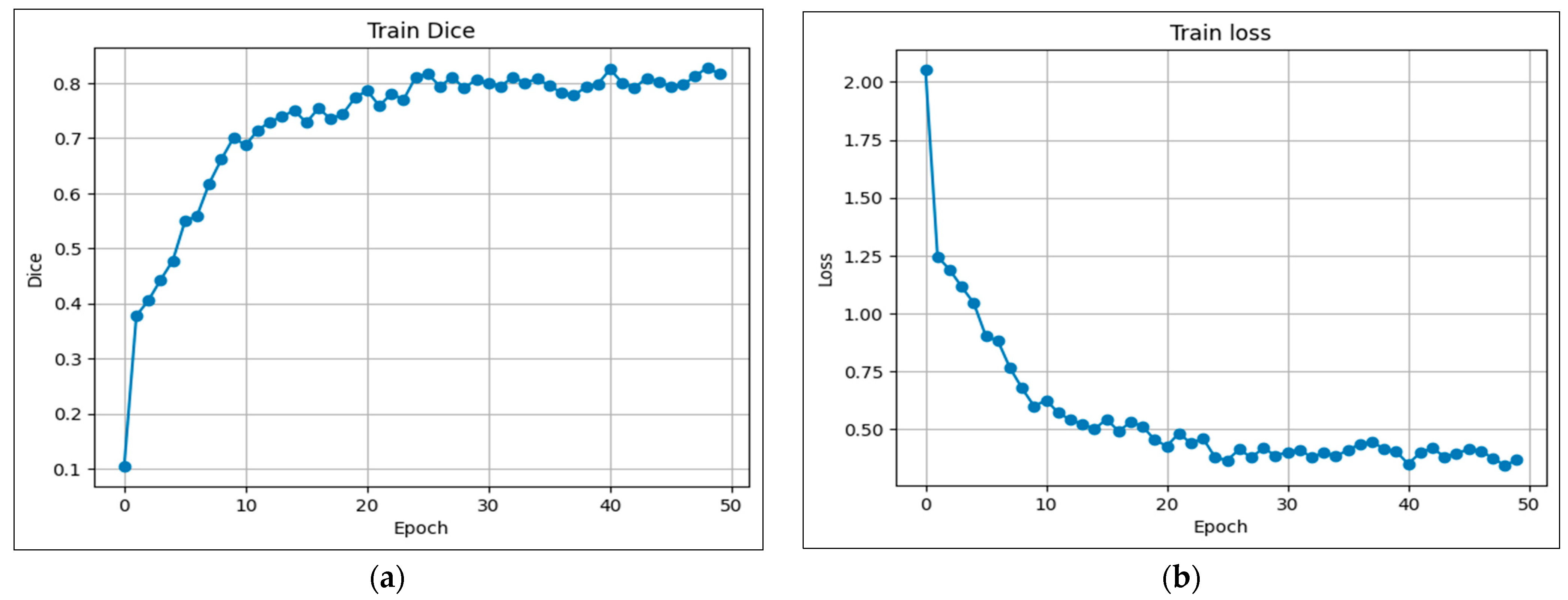
Following these procedures, our model was trained on the BraTS 2020 dataset. As described in Section 4.2, this dataset includes annotations for three distinct regions: class 1 denotes the enhancing tumor (ET), class 2 corresponds to the tumor core (TC), and class 3 indicates the whole tumor (WT). The evolution of the training performance is illustrated in Figure 5a,b over 50 training epochs. As shown in Figure 5b, the training loss decreased steadily from approximately 2.06 at epoch 0 to around 0.36 at epoch 50, indicating effective optimization of the model parameters and convergence of the learning process. Concurrently, the training Dice coefficient shown in Figure 5a rose from around 0.10 to 0.83, demonstrating improved segmentation performance as training progresses. This significant increase indicates the model’s ability to progressively learn to distinguish the complex tumor regions from the background. The steady training performance indicates that our proposed architecture is robust and effective at capturing crucial spatial and contextual features in MRI scans, which is essential for precise brain tumor segmentation.

Figure 5. Evolution of coefficients during training: (a) Dice; (b) Loss.

5.2. Performance Evaluation

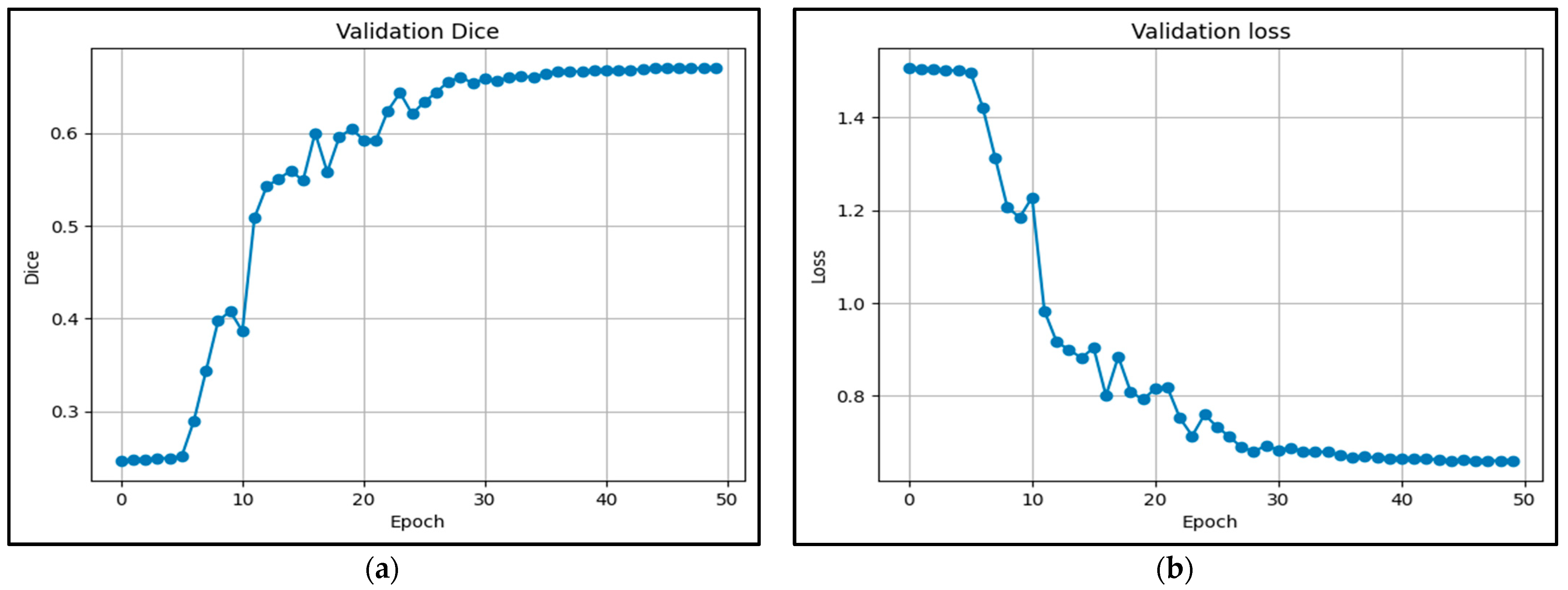
This section presents a detailed evaluation of the segmentation performance of our proposed hybrid model on the BraTS 2020 dataset using multiple metrics and region-specific analysis. We first present the validation dynamics and the evolution of loss and the Dice coefficient. Figure 6 shows the validation curves over 50 epochs, which reveal stable convergence and favorable learning behavior. The validation loss decreased from approximately 1.4 to below 0.5 (Figure 6b), while the validation Dice coefficient increased from 0.25 to above 0.7 (Figure 6a), indicating effective generalization with no signs of overfitting.

Figure 6. Evolution of coefficients during validation: (a) Dice; (b) Loss.

To further evaluate the segmentation results, we focused on three tumor subregions: enhancing tumor (ET), tumor core (TC), and whole tumor (WT) using confusion matrices, providing insights into the model’s segmentation capabilities for each region. As described in Figure 7a, the model correctly identified 7601 enhancing tumor voxels out of 7934 total, resulting in an accuracy of 99.89%, which indicates it was highly effective at detecting these tumors. Similarly, for the TC region, the model achieved 99.91% accuracy with 19,437 true positives, demonstrating a strong ability to identify core tumor tissues, as shown in Figure 7b. For the WT region, the WT was effectively segmented with 99.66% accuracy, supported by 60,825 true positives and moderate rates of false positives and negatives, as reported in Figure 7c. To complement this region-specific analysis, we computed the global confusion matrix in a four-class setting, which confirmed the model’s capacity to distinguish between different tumor tissues and healthy voxels. The results in Table 4 show that the model achieved a perfect accuracy of 99.56%, with an average Dice coefficient of 77.43% (STD = 0.0757) and a mean Intersection over Union (IoU) of 71.69% (STD = 0.0727). These standard deviation values indicate that the model performance is not only high on average but also consistent and robust across different cases. Overall, these results indicate that the proposed hybrid model effectively generalizes to unseen data while maintaining reliable segmentation precision across tumor subregions, even in complex cases.

Figure 7. Confusion matrices (TN, FP, FN, TP) for each subregion: (a) WT, (b) TC, (c) WT.

Table 4. Global confusion matrix (4 classes, 0–3).

Actual Predicted	Background (0)	ET (1)	TC (2)	WT (3)
Background (0)	7,776,535	35	15,250	1176
ET (1)	1458	7494	1361	3033
TC (2)	8014	91	38,175	793
WT (3)	1027	1309	968	7601
Global Accuracy	99.56%
Average DSC	77.43%
STD DSC	0.0727
Average IoU	71.69%
STD IoU	0.0757

5.3. Qualitative Visualization

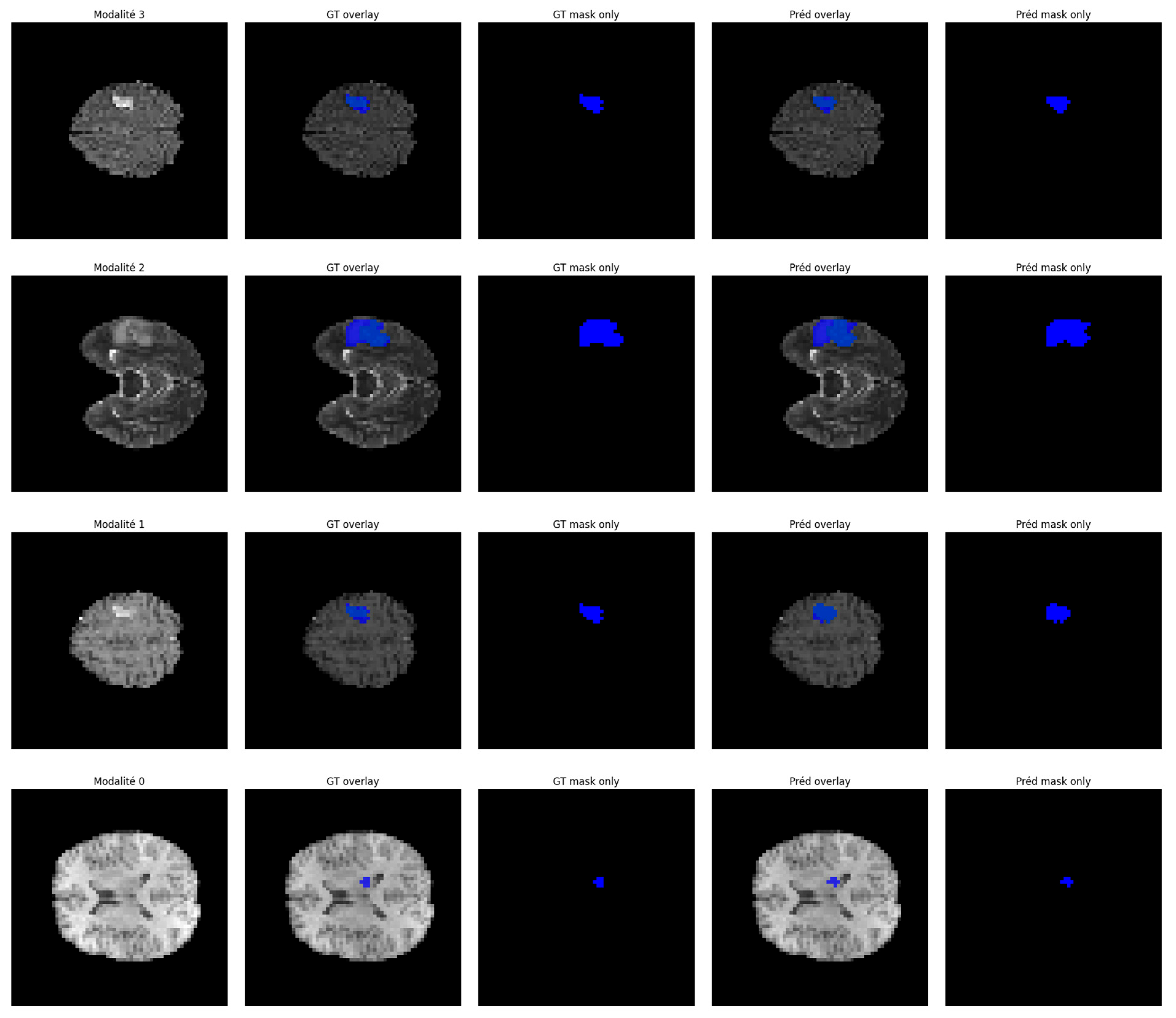
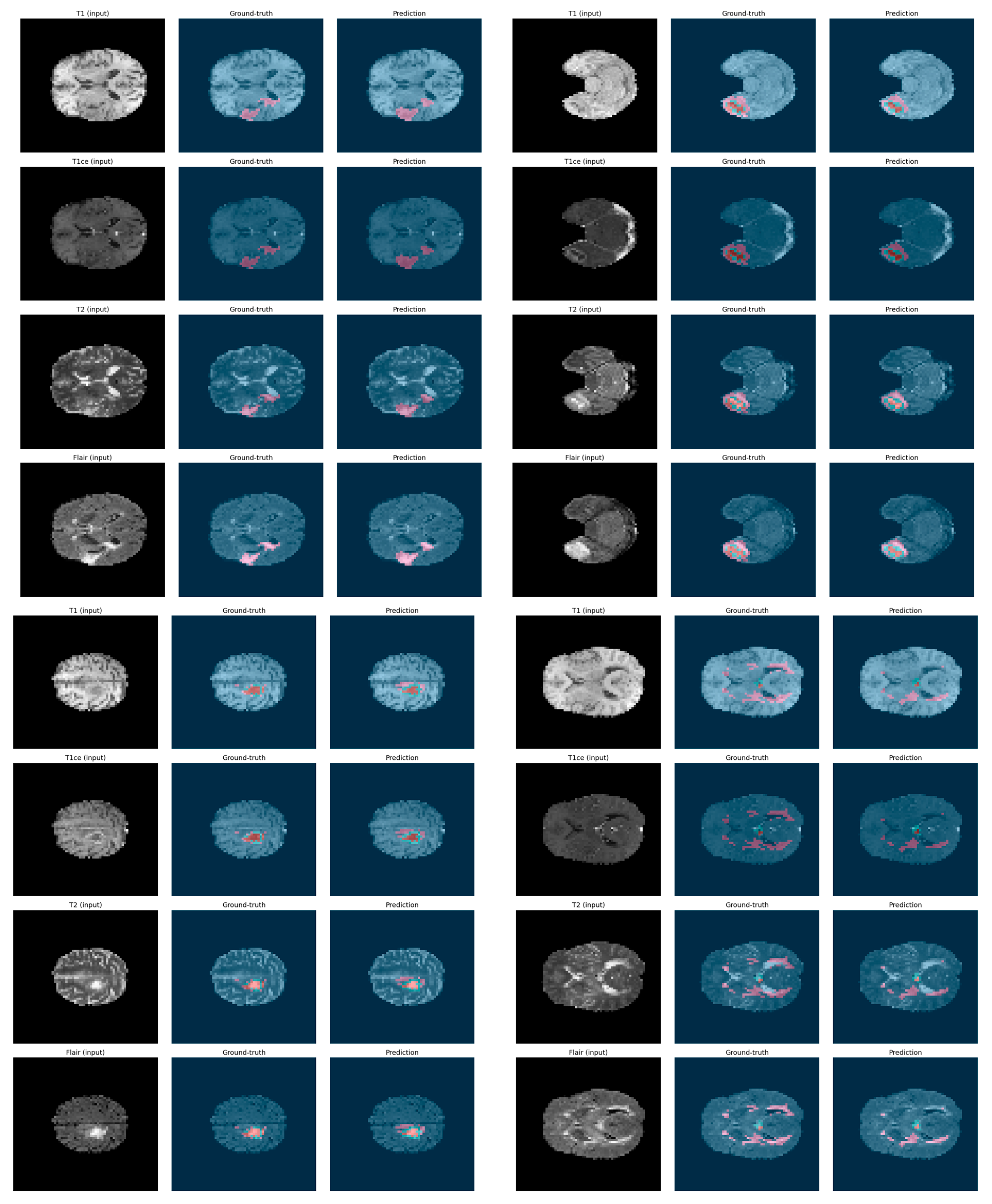
To further demonstrate the effectiveness of our proposed segmentation approach, we present a qualitative visualization of the results in Figure 8 and Figure 9. Figure 8 shows the segmentation results on 3D patches extracted from the four MRI modalities: T1, T1ce, T2, and FLAIR, which are encoded as 0, 1, 2, and 3, respectively. From left to right, the figure displays each modality, followed by the ground truth mask and the predicted segmentation mask. As can be observed, in several instances, the predicted segmentation closely matches the ground truth, confirming the model’s robustness and generalization across diverse cases. In Figure 9, we present examples of segmentation output on four modalities. Each row corresponds to a specific MRI modality, with the corresponding ground truth and the segmentation output generated by our model. The segmentation masks highlight tumor subregions using distinct colors: pink indicates enhancing tumor areas, while blue represents other subregions (such as edema or necrotic core, depending on the ground truth). The figure provides an intuitive understanding of the model’s consistency across modalities. It can be observed that the predicted masks closely follow the anatomical and pathological boundaries visible in each modality, demonstrating the model’s ability to effectively leverage multimodal information through fusion.

Figure 8. Segmentation results on multimodal MRI patches (T1, T1ce, T2, FLAIR).

Figure 9. Examples of segmentation output on 4 modalities: ground truth vs. prediction.

To sum up, both figures show that our model achieves a high level of visual alignment with the ground truth, which supports the quantitative results and demonstrates its robustness in handling complex tumor shapes and varying image contrast.

5.4. Comparison with State-of-the-Art

In this work, we compared our hybrid model with a selection of state-of-the-art methods, including various U-Net variants and Vision transformer-based models. The comparative experiments are presented in the following Table 5.

Table 5. Comparison of segmentation results with state-of-the art methods.

Methods	DSC (%)				IoU (%)
	ET	TC	WT	Average	ET	TC	WT	Average
U-Net [26]	60.0	62.0	80.0	67.33	42.0	52.0	67.0	53.66
VGG-19 + Decoder [22]	81.32	75.13	61.66	72.70	44.57	60.17	68.53	57.75
SwinUnet [46]	65.1	66.1	77.0	69.4	46.4	51.9	65.2	54.5
UNETR [38]	58.5	76.1	78.9	71.16	41.33	61.42	65.13	55.96
M-Unet [29]	66.00	72.00	87.00	75.00	49.25	56.25	76.99	60.83
TranBTS [37]	57.40	73.50	77.90	69.6	40.25	58.10	63.80	54.04
TransUnet [47]	54.20	68.40	70.60	64.4	37.17	52.01	54.55	47.91
Our Method	66.97	80.97	84.35	77.43	60.93	74.45	79.69	71.69

To demonstrate the superiority of our model over similar methods, we first compared it with U-Net-based models, such as U-Net [30], VGG-19 + Decoder [22], and M-Unet [29]. Our model achieved the highest average DSC score of 77.43% (STD = 0.0757), outperforming U-Net (67.33%) by approximately 10%, M-Unet (75.00%) by +2.43%, and VGG-19+Decoder (72.70%) by 4.73%. In terms of Intersection over Union (IoU), our model achieves an average of 71.69% (STD = 0.0727), surpassing U-Net, M-Unet, and VGG-19+Decoder, which obtained 60.83%, 54.5%, and 55.96%, with improvements of +10.86%, +17.19%, and +15.73%, respectively. These standard deviation values indicate that the model’s performance is not only high on average but also consistent across different cases.

Additionally, relative to Transformer-based architectures like SwinUnet, UNETR, and TranBTS, our model remains highly competitive. Compared to SwinUnet, which achieves 69.4% (DSC) and 54.5% (IoU), our model improves by +8.03% and +17.19%, respectively. Similarly, over UNETR (71.16% DSC, 55.96% IoU), our model achieves +6.27% and +15.73% improvement. Moreover, when compared to TransBTS introduced by Wang et al. [37], the proposed model obtains higher DSC scores across the WT, ET, and TC regions, further confirming its effectiveness and competitiveness. TranBTS reported an average DSC of 69.6% and IoU of 54.04%, which are notably lower than those obtained by our method. Finally, compared to TransUNet, another well-known Transformer-based segmentation architecture, our model demonstrates substantial improvements as well. TransUNet reports an average DSC of 64.4% and IoU of 47.91%, resulting in relative gains of +13.03% and +23.78%, respectively. These comparative results clearly highlight the superior performance and robustness of our proposed model across various benchmarks and segmentation regions. Note that all the underlined IoU values in Table 5, particularly those for the WT, TC, and ET regions, were manually calculated by us using the standard formula derived from the Dice Similarity Coefficient, as these values were not directly reported in the original studies.

5.5. Impact of the Multimodalities

The proposed model benefits significantly from the integration of multimodal MRI data, which provides a more detailed and complementary representation of brain tumor features. This integration enables the network to access a more comprehensive pathological overview, improving its ability to identify and distinguish between tumor subregions. For this purpose, our model adopts a hybrid fusion strategy. Initially, all four modalities are normalized and stacked along the channel axis, enabling early fusion, where the network can learn spatial and cross-modal correlations from the input. Later in the architecture, we applied a hybrid late fusion method by concatenating local (U-Net) and global (ViT) features to improve the detection of fine tumor boundaries and diffuse tumor structures. Additionally, the transformer-based attention mechanism in the 3D-ViT module enhances this multimodal analysis by capturing interactions across different modalities. For instance, an abnormal intensity in a FLAIR patch can be reinforced by matching enhancement observed in T1ce. This cross-modal interaction improves the model’s ability to differentiate tumor tissue from surrounding edema.

Quantitative and qualitative segmentation results demonstrate the concrete advantages of this multimodal design. Compared to a single modality 3D U-Net baseline, our model improves the Dice score by +4% for enhancing tumor (ET) and +3% for whole tumor (WT) (edema) detection. These benefits demonstrate that multimodality is a powerful tool for enhancing practical performance, not just a theoretical concept. Finally, the proposed architecture is modular and flexible, allowing for future integration of additional imaging modalities, such as PET or CT. The transformer block can also be replaced or deepened independently, without altering the U-Net backbone. This flexibility opens the door to broader clinical applications and adaptation to diverse multimodal scenarios beyond MRI.

6. Conclusions

In conclusion, we have proposed a novel hybrid framework for brain tumor segmentation in MRI scans, combining the strengths of 3D U-Net and 3D ViT. The proposed model integrates local spatial features from a 3D U-Net and global contextual information from 3D ViT through a dedicated fusion strategy based on upsampling and convolutional refinement to enhance accurate and robust segmentation of complex tumor structures.

Evaluated on the BraTS 2020 dataset, it achieved a Dice score of 84.35% for Whole Tumor, 80.97% for Tumor Core, and 66.97% for Enhancing Tumor. The corresponding IoU values were 79.69%, 74.45%, and 60.93%. The overall accuracy reached 99.56%. In addition, the model obtained an average Dice of 77.43% (STD of 0.0727) and an average IoU of 71.69% (STD of 0.0757), indicating not only strong segmentation performance but also stable behavior across different cases.

Despite these promising outcomes, several limitations should be noted. Our model, validated only on BraTS 2020, requires substantial computational resources and is sensitive to preprocessing choices. In the future, we plan to extend evaluation to additional datasets, improve efficiency, and release a detailed implementation to support reproducibility.

References

1. Litjens, G.; Kooi, T.; Bejnordi, B.E.; Setio, A.A.A. A survey on deep learning in medical image analysis. Med. Image Anal. 2017, 42, 60–88. [Google Scholar] [CrossRef] [PubMed]
2. Shen, D.; Wu, G.; Suk, H.-I. Deep Learning in Medical Image Analysis. Annu. Rev. Biomed. Eng. 2017, 19, 221–248. [Google Scholar] [CrossRef] [PubMed]
3. Rayed, M.E.; Islam, S.S.; Niha, S.I.; Jim, J.R.; Kabir, M.M.; Mridha, M. Deep learning for medical image segmentation: State-of-the-art advancements and challenges. Inform. Med. Unlocked 2024, 47, 101504. [Google Scholar] [CrossRef]
4. Sun, W.; Song, C.; Tang, C.; Pan, C.; Xue, P.; Fan, J.; Qiao, Y. Performance of deep learning algorithms to distinguish high-grade glioma from low-grade glioma: A systematic review and meta-analysis. iScience 2023, 26, 106815. [Google Scholar] [CrossRef]
5. Hamdaoui, F.; Sakly, A. Automatic diagnostic system for segmentation of 3D/2D brain MRI images based on a hardware architecture. Microprocess. Microsyst. 2023, 98, 104814. [Google Scholar] [CrossRef]
6. Ghribi, F.; Hamdaoui, F. Innovative Deep Learning Architectures for Medical Image Diagnosis: A Comprehensive Review of Convolutional, Recurrent, and Transformer Models. Vis. Comput. 2025, 1–26. [Google Scholar] [CrossRef]
7. Xiao, H.; Li, L.; Liu, Q.; Zhu, X.; Zhang, Q. Transformers in medical image segmentation: A review. Biomed. Signal Process. Control 2023, 84, 104791. [Google Scholar] [CrossRef]
8. El-Taraboulsi, J.; Cabrera, C.P.; Roney, C.; Aung, N. Deep neural network architectures for cardiac image segmentation. Artif. Intell. Life Sci. 2023, 4, 100083. [Google Scholar] [CrossRef]
9. Anand, V.; Gupta, S.; Koundal, D.; Nayak, S.R.; Barsocchi, P.; Bhoi, A.K. Modified U-NET Architecture for Segmentation of Skin Lesion. Sensors 2022, 22, 867. [Google Scholar] [CrossRef]
10. Dong, X.; Lei, Y.; Wang, T.; Thomas, M.; Tang, L.; Curran, W.J.; Liu, T.; Yang, X. Automatic multiorgan segmentation in thorax CT images using U-net-GAN. Med. Phys. 2019, 46, 2157–2168. [Google Scholar] [CrossRef]
11. Azad, R.; Kazerouni, A.; Heidari, M.; Aghdam, E.K.; Molaei, A.; Jia, Y.; Jose, A.; Roy, R.; Merhof, D. Advances in medical image analysis with vision Transformers: A comprehensive review. Med. Image Anal. 2024, 91, 103000. [Google Scholar] [CrossRef]
12. Jiang, Y.; Dong, J.; Cheng, T.; Zhang, Y.; Lin, X.; Liang, J. iU-Net: A hybrid structured network with a novel feature fusion approach for medical image segmentation. BioData Min. 2023, 16, 5. [Google Scholar] [CrossRef]
13. Bayoudh, K.; Hamdaoui, F.; Mtibaa, A. An Attention-based Hybrid 2D/3D CNN-LSTM for Human Action Recognition. In Proceedings of the 2022 2nd International Conference on Computing and Information Technology, ICCIT, Tabuk, Saudi Arabia, 25–27 January 2022; pp. 97–103. [Google Scholar]
14. Zhang, J.; Li, F.; Zhang, X.; Wang, H.; Hei, X. Automatic Medical Image Segmentation with Vision Transformer. Appl. Sci. 2024, 14, 2741. [Google Scholar] [CrossRef]
15. Al-hammuri, K.; Gebali, F.; Kanan, A.; Chelvan, I.E.T. Vision transformer architecture and applications in digital health: A tutorial and survey. Vis. Comput. Ind. Biomed. Art 2023, 6, 14. [Google Scholar] [CrossRef] [PubMed]
16. Azad, R.; Heidari, M.; Wu, Y.; Merhof, D. Contextual Attention Network: Transformer Meets U-Net. In Proceedings of the 13th International Workshop, MLMI 2022, Singapore, 18 September 2022. [Google Scholar]
17. Chen, B.; He, T.; Wang, W.; Han, Y.; Zhang, J.; Bobek, S.; Zabukovsek, S.S. MRI Brain Tumour Segmentation Using Multiscale Attention U-Net. Informatica 2024, 35, 751–774. [Google Scholar] [CrossRef]
18. Tan, M.; Le, Q.V. MixConv: Mixed Depthwise Convolutional Kernels. arXiv 2019, arXiv:1907.09595. [Google Scholar] [CrossRef]
19. Feng, S.; Zhao, H.; Shi, F.; Cheng, X.; Wang, M.; Ma, Y.; Xiang, D.; Zhu, W.; Chen, X. CPFNet: Context Pyramid Fusion Network for Medical Image Segmentation. IEEE Trans. Med. Imaging 2020, 39, 3008–3018. [Google Scholar] [CrossRef]
20. Bousselham, W.; Thibault, G.; Pagano, L.; Machireddy, A.; Gray, J.; Chang, Y.H.; Song, X. Efficient Self-Ensemble for Semantic Segmentation. arXiv 2022, arXiv:2111.13280. [Google Scholar] [CrossRef]
21. Aboussaleh, I.; Riffi, J.; El Fazazy, K.; Mahraz, M.A.; Tairi, H. Efficient U-Net Architecture with Multiple Encoders and Attention Mechanism Decoders for Brain Tumor Segmentation. Diagnostics 2023, 13, 872. [Google Scholar] [CrossRef]
22. Rehman, M.U.; Cho, S.; Kim, J.H.; Chong, K.T. BU-Net: Brain Tumor Segmentation Using Modified U-Net Architecture. Electronics 2020, 9, 2203. [Google Scholar] [CrossRef]
23. Bakas, S.; Reyes, M.; Jakab, A.; Bauer, S.; Rempfler, M. Identifying the Best Machine Learning Algorithms for Brain Tumor Segmentation, Progression Assessment, and Overall Survival Prediction in the BRATS Challenge. arXiv 2018, arXiv:1811.02629. [Google Scholar] [CrossRef]
24. Menze, B.H.; Jakab, A.; Bauer, S.; Kalpathy-Cramer, J.; Farahani, K.; Kirby, J. The Multimodal Brain Tumor Image Segmentation Benchmark (BRATS). IEEE Trans. Med. Imaging 2014, 34, 1993–2024. [Google Scholar] [CrossRef]
25. Ghosh, S.; Chaki, A.; Santosh, K. Improved U-Net architecture with VGG-16 for brain tumor. Phys. Eng. Sci. Med. 2021, 44, 703–712. [Google Scholar] [CrossRef]
26. Mazurowski, M.A.; Clark, K.; Czarnek, N.M.; Shamsesfandabadi, P.; Peters, K.B.; Saha, A. Radiogenomics of lower-grade glioma: Algorithmically-assessed tumor shape is associated with tumor genomic subtypes and patient outcomes in a multi-institutional study with The Cancer Genome Atlas data. J. Neurooncol. 2017, 133, 27–35. [Google Scholar] [CrossRef]
27. Nizamani, A.H.; Chen, Z.; Nizamani, A.A.; Bhatti, U.A. Advance brain tumor segmentation using feature fusion methods with deep U-Net model with CNN for MRI data. J. King Saud Univ.-Comput. Inf. Sci. 2023, 35, 101793. [Google Scholar] [CrossRef]
28. Zhao, L.; Ma, J.; Shao, Y.; Jia, C.; Zhao, J.; Yuan, H. MM-UNet: A multimodality brain tumor segmentation network in MRI images. Front. Oncol. 2022, 12, 950706. [Google Scholar] [CrossRef]
29. Ronneberger, O.; Fischer, P.; Brox, T. U-Net: Convolutional Networks for Biomedical. In Proceedings of the 18th International Conference on Medical Image Computing and Computer—Assisted Intervention, Munich, Germany, 5–9 October 2015; pp. 234–241. [Google Scholar]
30. Oktay, O.; Schlemper, J.; Le Folgoc, L.; Lee, M.; Heinrich, M.; Misawa, K.; Mori, K.; McDonagh, S.; Hammerla, N.Y.; Kainz, B.; et al. Attention U-Net: Learning Where to Look for the Pancreas. arXiv 2018, arXiv:1804.03999. [Google Scholar] [CrossRef]
31. Kaur, A.; Singh, Y.; Chinagundi, B. ResUNet + +: A comprehensive improved UNet + + framework for volumetric semantic segmentation of brain tumor MR image. Envol. Syst. 2024, 15, 1567–1585. [Google Scholar] [CrossRef]
32. Butt, M.A.; Jabbar, A.U. Hybrid Multihead Attentive Unet-3D for Brain Tumor Segmentation. arXiv 2024, arXiv:2405.13304. [Google Scholar] [CrossRef]
33. Badrinarayanan, V.; Kendall, A.; Cipolla, R. SegNet: A Deep Convolutional Encoder-Decoder Architecture for Image Segmentation. IEEE Trans. Pattern Anal. Mach. Intell. 2017, 39, 2481–2495. [Google Scholar] [CrossRef] [PubMed]
34. Long, J.; Shelhamer, E.; Darrell, T. Fully convolutional networks for semantic segmentation. In Proceedings of the 2015 IEEE Conference on Computer Vision and Pattern Recognition (CVPR), Boston, MA, USA, 7–12 June 2015; pp. 3431–3440. [Google Scholar]
35. Huang, G.; Liu, Z.; Van Der Maaten, L.; Weinberger, K.Q. Densely Connected Convolutional Networks. In Proceedings of the 2017 IEEE Conference on Computer Vision and Pattern Recognition (CVPR), Honolulu, HI, USA, 21–26 July 2017; pp. 2261–2269. [Google Scholar]
36. Wang, W.; Chen, C.; Ding, M.; Yu, H.; Zha, S.; Li, J. TransBTS: Multimodal Brain Tumor Segmentation Using Transformer. In Proceedings of the Medical Image Computing and Computer Assisted Intervention—MICCAI 2021: 24th International Conference, Strasbourg, France, 27 September–1 October 2021. [Google Scholar]
37. Hatamizadeh, A.; Tang, Y.; Nath, V.; Yang, D. UNETR: Transformers for 3D Medical Image Segmentation. In Proceedings of the 2022 IEEE/CVF Winter Conference on Application of Computer Vision, Waikoloa, HI, USA, 3–8 January 2022; pp. 574–584. [Google Scholar]
38. Landman, B.; Xu, Z.; Igelsias, J.; Styner, M.; Langerak, T.; Klein, A. Multi-Atlas Labeling Beyond the Cranial Vault—Workshop and Challenge. In Proceedings of the MICCAI, Munich, Germany, 5–9 October 2015. [Google Scholar] [CrossRef]
39. Simpson, A.L.; Antonelli, M.; Bakas, S.; Bilello, M.; Farahani, K.; van Ginneken, B.; Kopp-Schneider, A.; Landman, B.A.; Litjens, G.; Menze, B.; et al. A large annotated medical image dataset for the development and evaluation of segmentation algorithms. arXiv 2017, arXiv:1902.09063. [Google Scholar]
40. Liu, H.; Dowdell, B.; Engelder, T.; Pulmano, Z.; Osa, N.; Barman, A. Glioblastoma Tumor Segmentation using an Ensemble of Vision Transformers. In Proceedings of the MICAD 2023, Cambridge, UK, 9–10 December 2023. [Google Scholar]
41. Bakas, S.; Sako, C.; Akbari, H.; Bilello, M.; Sotiras, A.; Shukla, G.; Rudie, J.D.; Santamaría, N.F.; Kazerooni, A.F.; Pati, S.; et al. The university of pennsylvania glioblastoma (upenn-gbm) cohort: Advanced mri, clinical, genomics, & radiomics. Sci. Data 2022, 9, 453. [Google Scholar] [CrossRef]
42. Nian, R.; Zhang, G.; Sui, Y.; Qian, Y.; Li, Q.; Zhao, M.; Li, J.; Gholipour, A.; Warfield, S.K. 3D Brainformer: 3D Fusion Transformer for Brain Tumor Segmentation. arXiv 2023, arXiv:2304.14508. [Google Scholar] [CrossRef]
43. Zhou, H.-Y.; Guo, J.; Zhang, Y.; Han, X.; Wang, L.; Yu, Y. nnFormer: Volumetric Medical Image Segmentation via a 3D Transformer. IEEE Trans. Image Process. 2023, 32, 4036–4045. [Google Scholar] [CrossRef] [PubMed]
44. Perera, S.; Navard, P.; Yilmaz, A. SegFormer3D: An Efficient Transformer for 3D Medical Image Segmentation. In Proceedings of the 2024 IEEE/CVF Conference on Computer Vision and Pattern Recognition Workshops (CVPRW), Seattle, WA, USA, 17–18 June 2024. [Google Scholar]
45. Liu, C.; Kiryu, H. 3D Medical Axial Transformer: A Lightweight Transformer Model for 3D Brain Tumor Segmentation. In Proceedings of the Medical Imaging with Deep Learning 2023, Nashville, TN, USA, 10–12 July 2023; Volume 227, pp. 799–813. [Google Scholar]
46. Cao, H.; Wang, Y.; Chen, J.; Jiang, D.; Zhang, X.; Tian, Q.; Wang, M. Swin-Unet: Unet-like Pure Transformer for Medical Image Segmentation. arXiv 2021, arXiv:2105.05537v1. [Google Scholar]
47. Chen, J.; Lu, Y.; Yu, Q.; Luo, X.; Adeli, E.; Wang, Y.; Lu, L.; Yuille, A.L.; Zhou, Y. TransUNet: Transformers Make Strong Encoders for Medical Image Segmentation. arXiv 2021, arXiv:2102.04306. [Google Scholar] [CrossRef]
Disclaimer/Publisher’s Note: The statements, opinions and data contained in all publications are solely those of the individual author(s) and contributor(s) and not of MDPI and/or the editor(s). MDPI and/or the editor(s) disclaim responsibility for any injury to people or property resulting from any ideas, methods, instructions or products referred to in the content.
Article Metrics
Citations
Article Access Statistics
Multiple requests from the same IP address are counted as one view.