Spatially Adaptive and Distillation-Enhanced Mini-Patch Attacks for Remote Sensing Image Object Detection

Abstract

Despite the remarkable success of Deep Neural Networks (DNNs) in Remote Sensing Image (RSI) object detection, they remain vulnerable to adversarial attacks. Numerous adversarial attack methods have been proposed for RSI; however, adding a single large-scale adversarial patch to certain high-value targets, which are typically large in physical scale and irregular in shape, is both costly and inflexible. To address this issue, we propose a strategy of using multiple compact patches. This approach introduces two fundamental challenges: (1) how to optimize patch placement for a synergistic attack effect, and (2) how to retain strong adversarial potency within size-constrained mini-patches. To overcome these challenges, we introduce the Spatially Adaptive and Distillation-Enhanced Mini-Patch Attack (SDMPA) framework, which consists of two key modules: (1) an Adaptive Sensitivity-Aware Positioning (ASAP) module, which resolves the placement challenge by fusing the model’s attention maps from both an explainable and an adversarial perspective to identify optimal patch locations, and (2) a Distillation-based Mini-Patch Generation (DMPG) module, which tackles the potency challenge by leveraging knowledge distillation to transfer adversarial information from large teacher patches to small student patches. Extensive experiments on the RSOD and MAR20 datasets demonstrate that SDMPA significantly outperforms existing patch-based attack methods. For example, against YOLOv5n on the RSOD dataset, SDMPA achieves an Attack Success Rate (ASR) of 88.3% using only three small patches, surpassing other patch attack methods.

1. Introduction

Remote sensing image (RSI) object detection plays a critical role in numerous real-world applications, including land resource monitoring, urban planning, environmental change detection, precision agriculture, and military surveillance. Deep learning techniques have significantly advanced in accuracy and robustness of object detection models in remote sensing scenes. Models such as YOLO, R-CNN, RetinaNet, DETR, and Swin Transformer have been widely applied to extract semantic information from high-resolution RSI, enabling accurate identification and localization of small, sparse, and densely distributed objects such as aircraft, vehicles, ships, and buildings.

Despite these advances, recent studies have shown that DNN-based object detectors are inherently vulnerable to adversarial attacks [1]. Among these, adversarial patch attacks have emerged as a particularly alarming threat. Unlike traditional pixel-level [2] attacks that introduce subtle perturbations across the entire image, adversarial patches are localized, designed to deceive a neural network’s prediction [3,4].

An adversarial patch attack typically involves crafting a region of noise or texture that, when overlaid onto an image [5,6], can mislead the detector into ignoring objects, as illustrated in Figure 1, misclassifying them, or detecting false positives. Compared to noise-based attacks, patch-based attacks are highly efficient and deployment-friendly, especially when full-image perturbation is infeasible.

Compared to general object detection scenarios, RSIs exhibit a significant span in target scales, which not only poses certain difficulties for conventional object detection but also introduces unique challenges for adversarial attacks—targets of different scales often lead to specific issues. Dong et al. [7] defined the target scales in RSI scenes as large, medium, and small, and conducted relevant statistical analyses. According to their research, small targets can account for approximately 60% in RSI. Although small targets dominate in RSI scenes, high-value large-scale targets (such as aircraft, oil tanks, and ships) are typically larger in physical dimensions. These large-scale targets are equally worthy of in-depth investigation, as deploying a single large-scale patch attack on them is often costly, conspicuous, and operationally inflexible, thereby limiting practical applications.

A straightforward solution is to reduce the patch size. However, simply downsizing the patch leads to weakened attack strength because the limited perturbation region may not inject sufficient adversarial signals into the network’s high-level feature representations.

To overcome the limitations of single, large patches, a promising direction is to employ multiple compact patches. To the best of our knowledge, our work is the first to systematically investigate this multi-mini-patch strategy for the complex task of object detection. This pioneering approach, however, introduces two fundamental challenges: optimizing patch placement for synergistic effects, and retaining adversarial potency within size-constrained patches.

In light of these issues, we propose the Spatially Adaptive and Distillation-Enhanced Mini-Patch Attack (SDMPA) framework. To solve the placement problem, we design the Adaptive Sensitivity-Aware Positioning (ASAP) module, which leverages a novel fusion of explainable and adversarial signals. To solve the potency problem, we use knowledge distillation for adversarial content generation, realized through our Distillation-based Mini-Patch Generation (DMPG) module. This is, to our knowledge, the first work to repurpose knowledge distillation as an offensive tool to enhance the attack strength of compact patches. The contributions of our work can be summarized as follows:

-

We propose a novel attack framework SDMPA for RSI object detection. To overcomes the impracticality of deploying a single, large-scale patch, we propose to generate multiple patches for adversarial attack.

-

We design the Adaptive Sensitivity-Aware Positioning (ASAP) module, which intelligently selects optimal patch locations by fusing the model’s explainable attention map with an adversarial gradient map. This synergistic approach ensures both effective placement and high attack potency.

-

We develop the Distillation-based Mini-Patch Generation (DMPG) module, which utilizes knowledge distillation to transfer adversarial knowledge from large teacher patches to smaller student patches. This mechanism effectively enhances the adversarial potency of the compact patches.

-

We conducted extensive experiments on the RSOD and MAR20 datasets. The results demonstrate that our SDMPA framework significantly outperforms existing patch-based attack methods by achieving a higher Attack Success Rate (ASR) with smaller adversarial patches.

2. Related Work

2.1. Adversarial Attack for Remote Sensing Image

Adversarial attacks have become a widely studied topic in the field of deep learning security [8]. Broadly speaking, these attacks can be categorized into two main types: pixel-level attacks [9], which apply imperceptible perturbations across an image to mislead the model’s prediction, and patch-level attacks [10], which introduce a localized and visually perceptible adversarial patch designed to disrupt object detection or classification [11]. In particular, patch-level attacks such as DPatch [12] and Natural Patch [13] have demonstrated significant effectiveness in general computer vision scenarios, posing realistic threats even in physical-world settings [14]. These approaches typically aim to craft universal or targeted patches that can be deployed without requiring image-specific tuning, thereby offering high flexibility and practicality [15].

However, most of these patch-based methods [16,17,18] are developed for natural image benchmarks such as COCO or Pascal VOC. When transferred to RSI, they exhibit substantial limitations. Unlike natural images, RSIs feature densely distributed small objects, complex background textures, high viewpoint variability, and varying spatial resolutions. These characteristics pose unique challenges to adversarial attack design [19]. As a result, there has been a growing body of research that focuses specifically on adversarial attacks tailored to remote sensing applications.

To address the specific demands of RSIs, a range of specialized attack strategies have been proposed [20]. These include noise-based attacks that introduce pixel-level perturbations optimized for satellite or aerial imagery, background-based attacks such as the Contextual Background Attack (CBA) [21], which manipulate the semantic surroundings of target objects, and patch-based methods like the Adversarial Patch Positioning Attack (APPA) [22]. Additionally, the Environmental Masking Attack (EMA) [23] integrates scene priors and environmental factors to boost patch stealth and robustness under remote sensing conditions. Li [24] proposed a physical adversarial patch attack against fine grained aircraft recognition.

Although these works have greatly advanced the study of adversarial attacks in remote sensing, they predominantly focus on a single-patch paradigm, which is often costly and inflexible for physical deployment [25,26]. However, early attempts revealed that effectively coordinating multiple patches in object detection is a non-trivial challenge. For instance, Tang et al. [27] explored multi-patch attacks in RSI object detection scenarios but failed to achieve stronger attack effectiveness compared to a single patch. This limitation was mainly due to their use of a random strategy for patch placement, which did not exploit the potential synergistic effects among patches.

A notable exception is the work by Huang et al. [28], who proposed a multi-mini-patch adversarial attack framework designed for remote sensing imagery. Their study represents an early and valuable attempt to move beyond single-patch strategies. Building upon their foundational work, we identify two key areas for further advancement.

First, their approach primarily focuses on image classification models, while the more complex and broadly applicable task of object detection remains an open challenge. Unlike classification, object detection involves both localization and classification, demanding more precise feature manipulation. Second, the methodology for generating adversarial content within compact patches was not the central focus of their study; while they introduced the concept of using multiple small patches, the challenge of retaining strong adversarial effects when downsizing the patch warrants deeper investigation. Our work aims to address these specific challenges by proposing a systematic approach to jointly optimize patch content and placement.

2.2. Knowledge Distillation

Since Hinton et al. [29] first proposed Knowledge distillation (KD), KD has emerged as a powerful paradigm for model compression and knowledge transfer. In recent years, KD has demonstrated remarkable success in a variety of computer vision tasks. For example, it has been used to compress large language–vision models [30], improve the precision of object detectors [31,32], and enhance performance in dense prediction tasks such as semantic segmentation [33].

More recently, researchers have begun to explore the integration of knowledge distillation into adversarial learning frameworks. In most of these efforts, KD is adopted as a defense mechanism. Specifically, robust teacher models—often trained on adversarial examples—are used to guide student models toward improved adversarial robustness [34]. By mimicking the teacher’s resilient behavior under attack, the student model can inherit resistance to various adversarial perturbations, thereby enhancing the system’s overall security. These methods have demonstrated significant gains in adversarial defense, especially in classification tasks.

However, the use of knowledge distillation in the context of adversarial attacks has only recently begun to be explored. Liu [35] leveraged KD to generate adversarial patches with enhanced visual concealment, aiming to make the perturbations less perceptible to human observers.

While they focus on improving patch stealth, our work addresses a different yet equally critical challenge: retaining strong adversarial potency within a severely limited pixel budget. To the best of our knowledge, our work is the first to systematically exploit knowledge distillation as a tool for generating multiple compact mini-patches that bridge the gap between deployability and attack strength, particularly for the complex task of remote sensing object detection. This strategic repurposing of KD not only enables improved attack efficiency but also opens up new possibilities for research in adversarial patch attacks.

3. Proposed Method

3.1. Overview

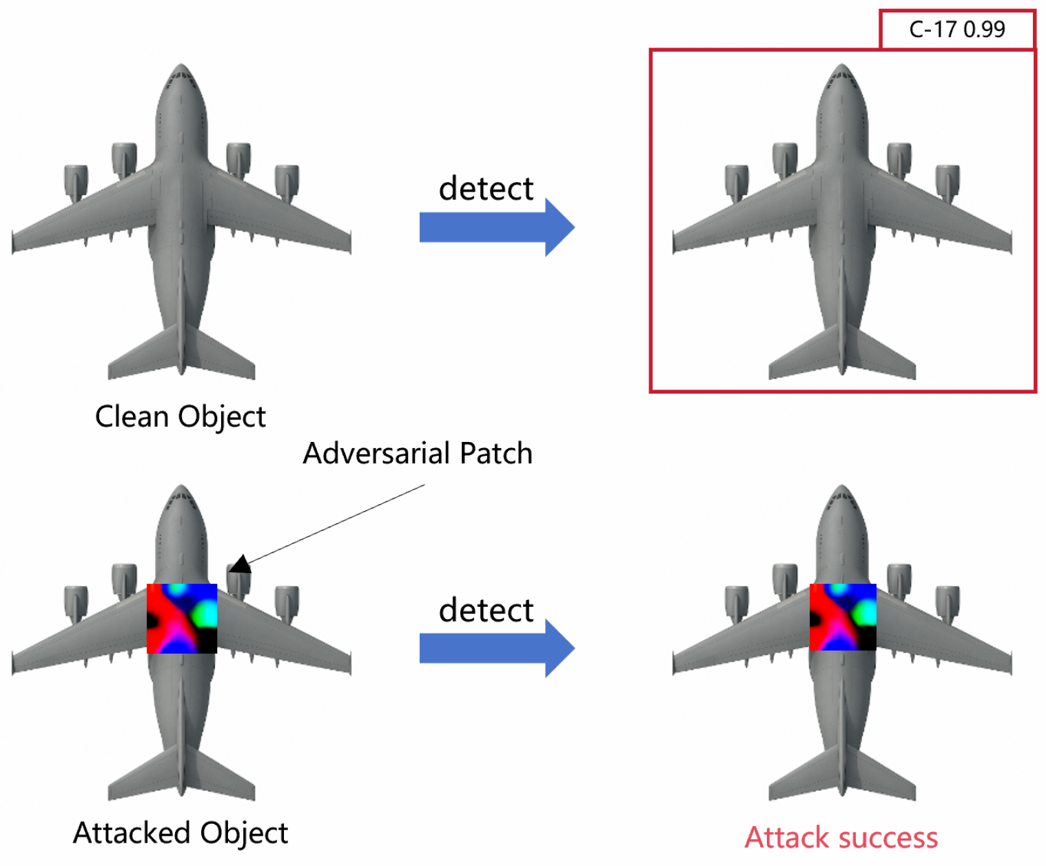
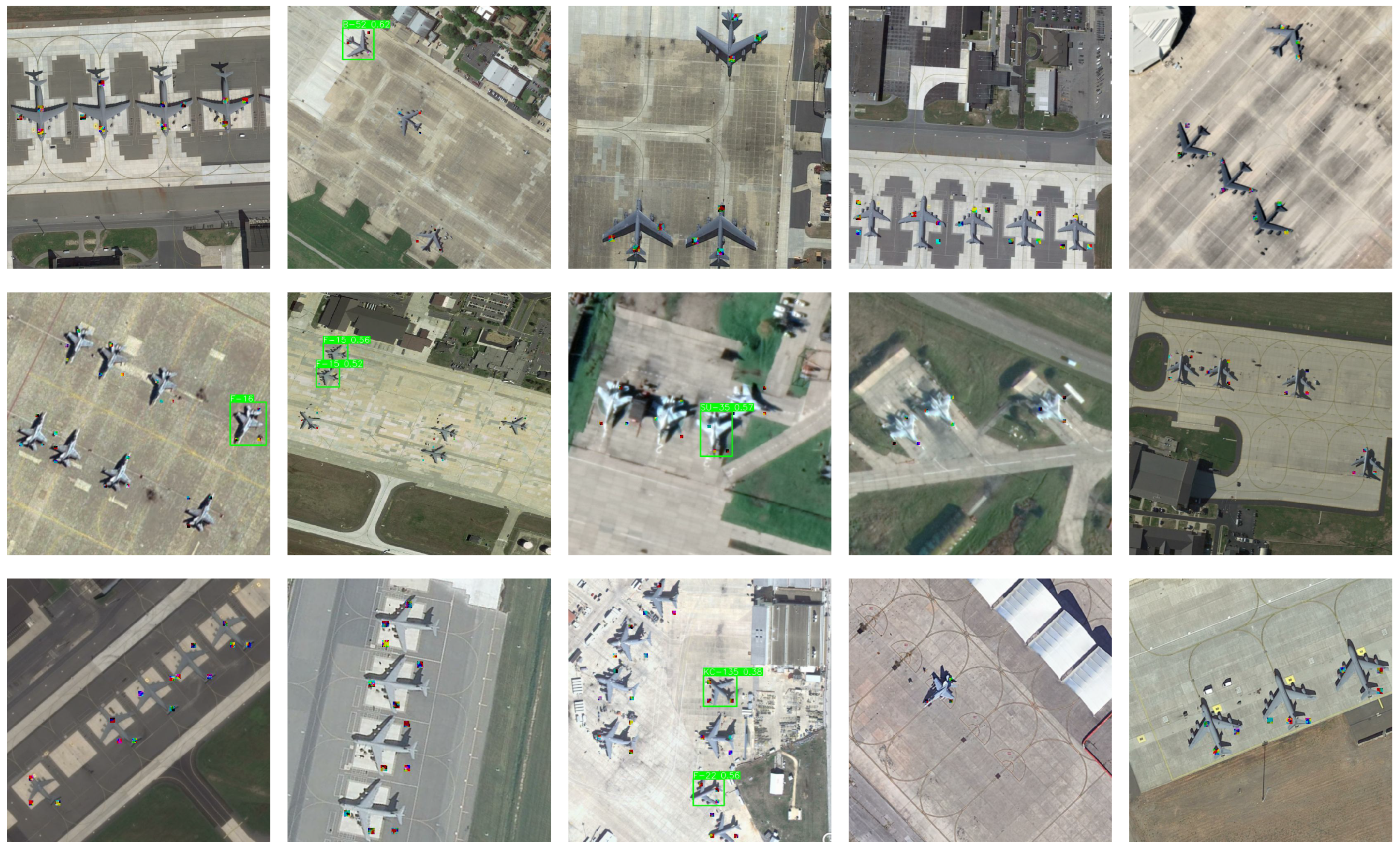
The Spatially Adaptive and Distillation-Enhanced Mini-Patch Attack (SDMPA) framework is designed to address the impracticality of deploying single, large adversarial patches against large-scale physical targets in RSI. As illustrated in Figure 2, our framework overcomes this by strategically using multiple compact patches, tackling the dual challenges of optimal patch placement and adversarial strength retention through two core components.

First, the ASAP module solves the collaborative positioning problem. Rather than selecting vulnerable points individually, ASAP identifies a complementary set of locations that produce a synergistic attack effect. It achieves this by fusing two sources of information: a inner model attention map ($M_i$) for explainable view guidance and a adversarial view gradient map ($M_a$) for pinpointing adversarial weak spots within those regions. This fusion ensures that patch locations possess both global importance and local attack efficiency.

Second, after ASAP determines the optimal locations, the Distillation-based Mini-Patch Generation (DMPG) module addresses the challenge of retaining attack potency in small patches. It employs a knowledge distillation strategy where a larger, more powerful “teacher” patch is first optimized at each designated location. This teacher’s adversarial knowledge is then transferred to a compact “student” patch via a specialized distillation loss function, guiding it to inherit potent attack characteristics despite its limited spatial budget. This combination of intelligent placement and guided generation allows SDMPA to achieve high attack success rates, making it a highly practical approach for real-world applications.

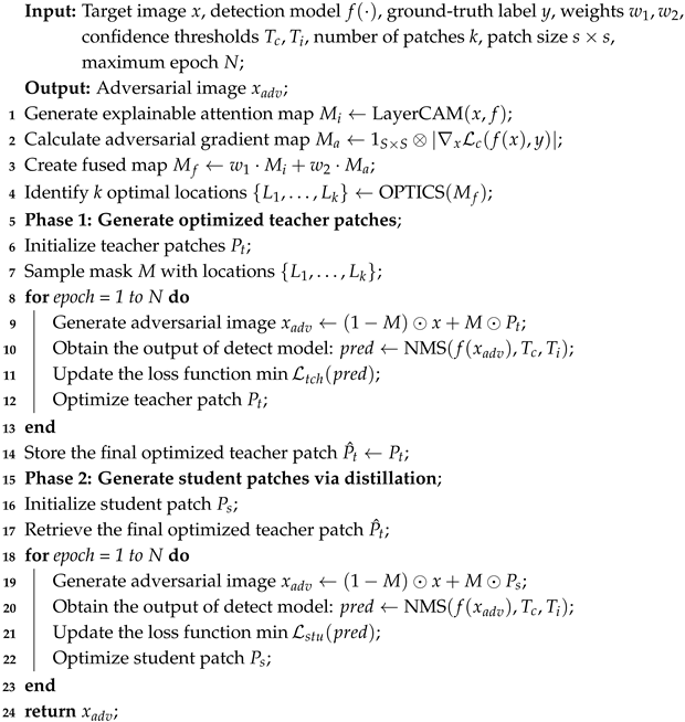
We provide a detailed description of the optimization procedures of the SDMPA approach in Algorithm 1. Specifically, given initial patch parameters, we first generate the explainable attention map $M_i$ using LayerCAM and compute the adversarial gradient map $M_a$, fusing them into $M_f$ to identify k optimal patch locations $\{L_1,\dots ,L_k\}$. Next, in Phase 1, we initialize the teacher patches $P_t$ and sample mask M, placing the patches on the clean image x to form the adversarial image $x_{adv}$. Subsequently, we feed the adversarial image into the target detection model f, extract predictions $pred$ via NMS, and use it as part of the teacher loss ${\mathcal{L}}_{tch}$. Then, we perform backpropagation to update the teacher patches $P_t$. Finally, we repeat the above steps until the end of the training process. In Phase 2, we use the distillation mechanism to transfer adversarial knowledge from the teacher patches to the student patches $P_s$, similarly generating $x_{adv}$, computing the student loss ${\mathcal{L}}_{stu}$ (including distillation loss), optimizing $P_s$, and repeating iterations to output the final adversarial image $x_{adv}$.

Algorithm 1: SDMPA.

3.2. Adaptive Sensitivity-Aware Positioning (ASAP) Module

The Adaptive Sensitivity-Aware Positioning (ASAP) module is designed to precisely identify multiple, high-value locations on a target for our novel multi-mini-patch attack strategy. Its core idea is that the optimal attack points should simultaneously possess both semantic importance, reflecting the model’s focus during normal recognition, and adversarial sensitivity, representing its vulnerabilities under attack. To this end, the ASAP module employs a dual-perspective fusion strategy to locate these critical regions.

First, we analyze the model’s focus from a standard perspective by examining its behavior on unperturbed inputs. We use the LayerCAM [36] method to generate the model’s internal attention map, denoted as $M_i$, while this map is rich in semantic information, highlighting the key regions the model relies on, it also has a low resolution and coarse granularity. Intuitively, perturbing these highly attended areas can most directly impact the model’s decision-making process.

However, as shown by Wu et al. [37], a model’s high-attention regions are not always equivalent to its adversarially vulnerable regions. Our multi-patch approach allows us to explore more complex attack patterns beyond targeting a single high-attention area. Adversarial perturbations can cause significant shifts in the model’s attention, and these shifted feature points represent the model’s sensitive areas from an adversarial perspective.

To capture these vulnerabilities from the adversarial perspective [38], we first generate an adversarial example by iteratively applying a small, imperceptible perturbation to the original sample. The number of iterations is empirically set to 10, with a step size $\alpha$ 0.001. The process for generating this adversarial example is defined as follows:

$$x_a^{(t+1)}={\mathrm{Clip}}_{x_a,ϵ}\left(x_a^{\left(t\right)}+\alpha ·\mathrm{sign}\left({\nabla }_{x_a^{\left(t\right)}}J(x_a^{\left(t\right)},y)\right)\right)$$

(1)

Next, we obtain the model’s attention map under adversarial conditions, which we define as the Adversarial Attention Map $M_a$. This map reveals the new, sensitive regions to which the model’s attention shifts when under attack. To obtain a more fine-grained attention map, it is generated as follows:

$$M_a=1_{S\times S}\otimes \left|{\nabla }_{x_a}{\mathcal{L}}_c(f\left(x_a\right),y)\right|$$

(2)

where ${\nabla }_{x_a}$ denotes the gradient of the loss function ${\mathcal{L}}_c$ with respect to the input image $x_a$, $1_{S\times S}$ is an all-one convolution kernel of size $S\times S$, and ⊗ represents the convolution operation. The kernel’s side length, S, is equal to the patch’s side length.

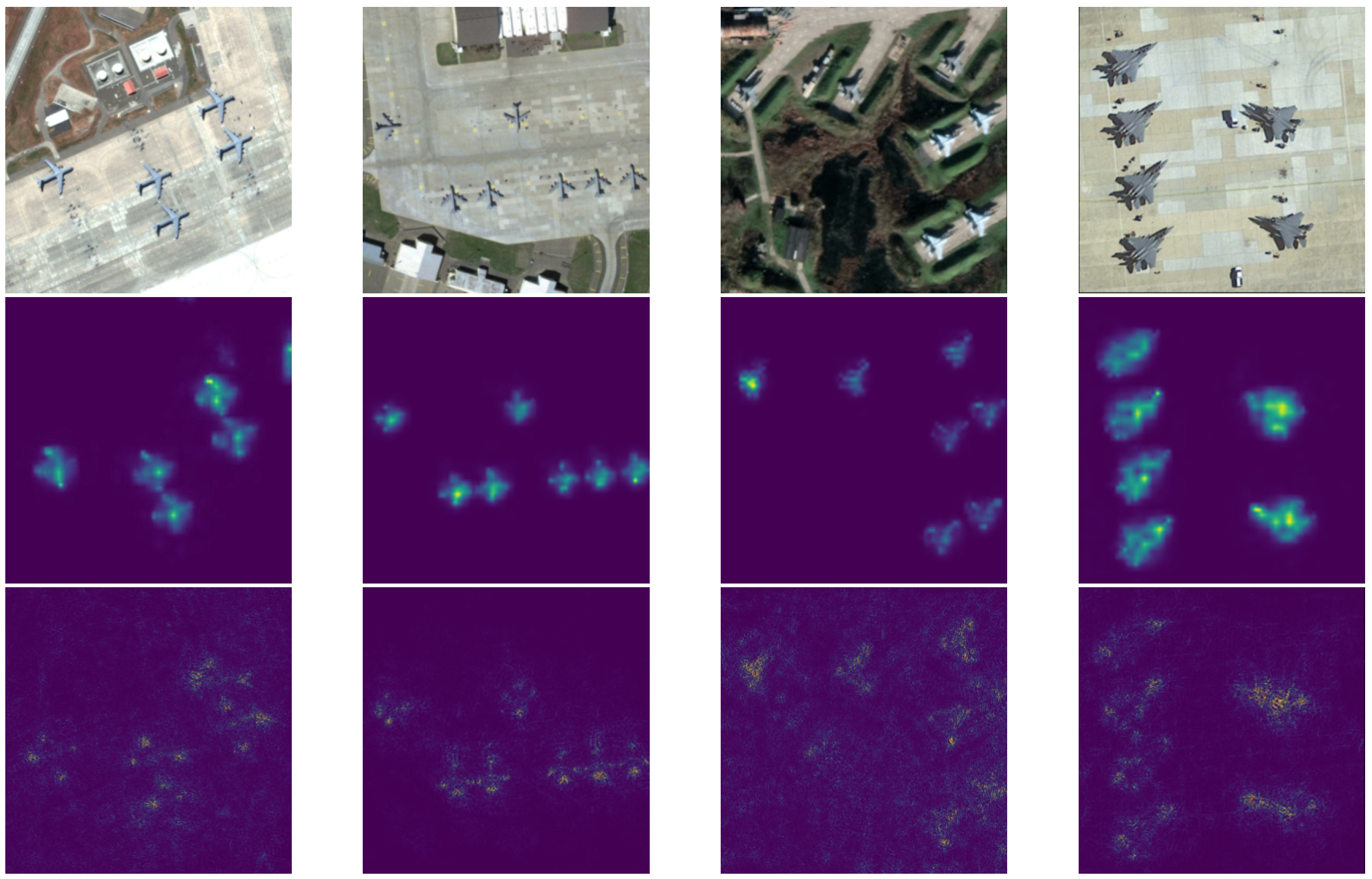
With these steps, we obtain two guidance maps that describe the model’s behavior from complementary perspectives: $M_i$ represents semantic importance, while $M_a$ reveals adversarial vulnerability. The illustration of $M_i$ and $M_a$ is shown in Figure 3. To find optimal locations that possess both attributes, we combine them through a weighted fusion:

$$M_f=w_1·M_i+w_2·M_a$$

(3)

Here, $w_1$ and $w_2$ are hyperparameters that balance the contribution of the two perspectives. Through preliminary experiments, we determined that a weighting of $w_1=0.6$ and $w_2=0.4$ provides an effective balance between the model’s standard attention and its adversarial sensitivities.

Finally, to extract k discrete and spatially distinct attack points from the continuous fused map $M_f$, we employ the Ordering Points To Identify the Clustering Structure (OPTICS) algorithm. This approach is adept at identifying high-density core regions, which we designate as the final patch locations to maximize synergistic effects. Before applying the algorithm, we convert the map into a weighted point set, where each pixel’s intensity determines its importance. To accommodate targets of varying scales, the algorithm’s key parameter max_eps are dynamically adjusted based on the pixel count within the target area.

Specifically, we first construct weighted coordinate data based on pixel intensity values. The pixel intensities are normalized to the range of 1–5 and used as repetition counts, so that high-intensity pixels are assigned higher importance weights during clustering. Then, the key parameters of the OPTICS algorithm are dynamically adjusted according to the number of valid pixels within the target region: when the number of pixels is fewer than 50, we set max_eps = 30; when the number of pixels is between 50 and 200, we set max_eps = 40; and when the number of pixels exceeds 200, we set max_eps = 50.

For cluster identification, we utilize the xi-steep extraction method with $xi=0.02$, a technique designed to automatically detect clusters by analyzing steep upward and downward shifts in the OPTICS reachability plot. Since this process yields cluster assignments rather than explicit centers, we then compute the weighted centroid $C_i$ for each valid cluster i:

$$C_i={\displaystyle \frac{{\sum }_{p\in {\mathrm{Cluster}}_i}I\left(p\right)·p}{{\sum }_{p\in {\mathrm{Cluster}}_i}I\left(p\right)}}$$

(4)

where p represents the pixel coordinates and $I\left(p\right)$ is its intensity. To select the most potent locations, we score each centroid based on its cluster’s total intensity and spatial compactness. In cases where the number of identified clusters is less than the required k, a supplementary strategy is activated. This strategy selects additional high-activation points from the remaining target area, ensuring that a sufficient number of spatially independent and optimally placed attack locations are always generated.

3.3. Distillation-Based Mini Patch Generation (DMPG) Module

Knowledge distillation is a well-known technique where a lightweight student model is trained by a more complex teacher model. Traditionally used for model compression, KD has been successfully applied in adversarial learning to enhance the robustness of models against adversarial perturbations. In the context of adversarial patch generation, we extend this concept to guide the optimization of compact patches. Instead of learning classification predictions, our goal is to offer a better training patch to compact patches by build the connection of strong adversarial patches. This allows the student patch to inherit the ability to perturb the model effectively while maintaining a small size, making it more deployable and harder to detect.

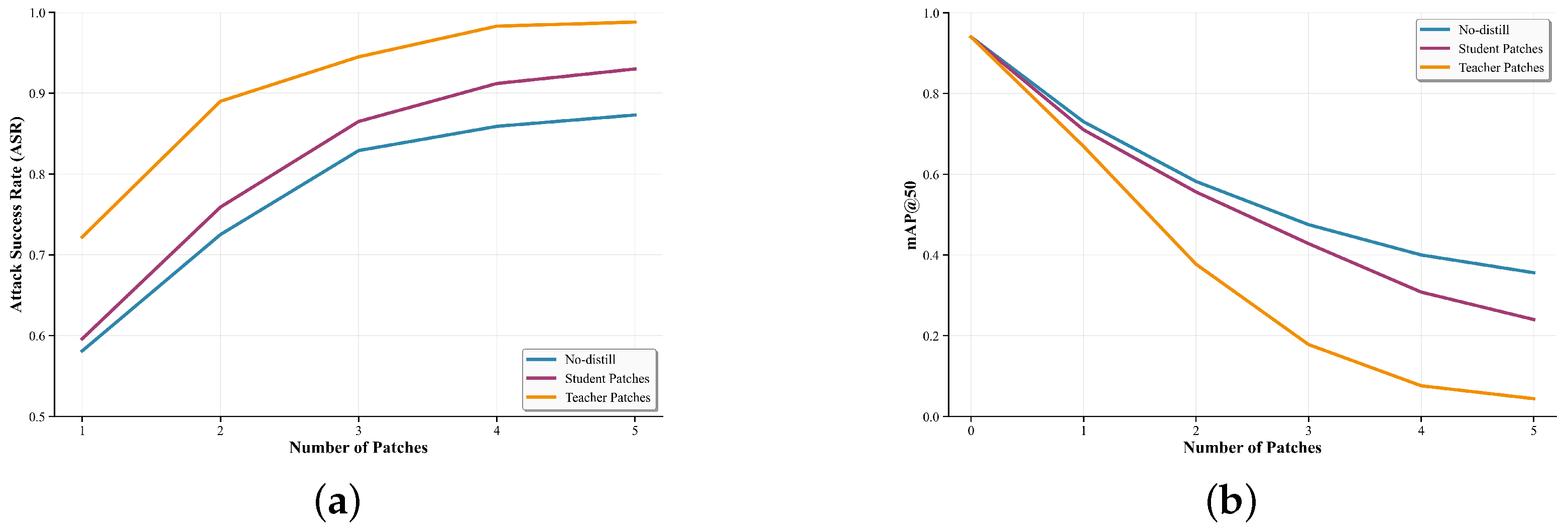
Figure 2 illustrates the core intuition behind the DMPG module: by leveraging a strong teacher patch as guidance, the student patch can obtain better attack information in the feature space, bridging the gap between weak and strong attacks while preserving compactness.

To implement this idea, we first generate larger teacher patches by optimization the teacher patch training loss ${\mathcal{L}}_{\mathrm{tch}}$. These teacher patches serve as high-capacity ability of adversarial knowledge. We then distill the adversarial knowledge from teacher patches into smaller student patches through loss function ${\mathcal{L}}_{\mathrm{distill}}$.

3.3.1. Teacher Patch Generation

The teacher patches, denoted as $P_t$, serve as a powerful knowledge source for the distillation process. Unlike the highly compact student patches, the teacher patches are generated with a larger size. The larger patch size not only means the bigger information capacity but also means it will be farther away from the ground truth in the high-dimensional space.

If the teacher patch is significantly larger than the student patch, the guidance effect may be weakened due to the substantial distribution gap between their feature representations in the high-dimensional space. The precise impact of the teacher–student size ratio will receive a detailed analysis in Section 4.4.3. The placement of these teacher patches follows the same spatial guidance as the student patches. Specifically, for each of the optimal locations identified by the ASAP module, we concurrently optimize a larger teacher patch and a smaller student patch. The optimization of the teacher patch is driven by three loss functions, each targeting a specific aspect of its performance:

• Detection Loss ${\mathcal{L}}_d$: This loss is designed to suppress the objectness confidence of predicted bounding boxes that correspond to ground-truth objects. To isolate relevant predictions from background noise that could hinder the optimization process, we first apply non-maximum suppression (NMS) to the detector’s raw output. Specifically, we configure the NMS with a confidence threshold of 0.001 and an IoU threshold of 0.1. This pre-processing step ensures that the loss function focuses squarely on suppressing the most salient object predictions, thereby training the patch to diminish the detector’s belief that a target is present.

  $${\mathcal{L}}_d={\displaystyle \frac{1}{N}}\sum _{i=1}^N\mathrm{obj}\left(i\right)$$

  (5)
  Here, $\mathrm{obj}\left(i\right)$ denotes the objectness score of the i-th predicted bounding box. Our goal is to directly minimize the detector’s objectness confidence for true objects. Other scoring components (e.g., classification confidence) are not considered in this loss, since reducing objectness alone often suffices for successful suppression.
• Total Variation Loss ${\mathcal{L}}_{tv}$: This loss promotes spatial smoothness within the patch, reducing pixel-level artifacts that could make the patch detectable by human observers. This smoothness ensures that the perturbation remains subtle and stealthy, as described by:

  $${\mathcal{L}}_{tv}=\sum _{i,j}\left[{(p_{i+1,j}-p_{i,j})}^2+{(p_{i,j+1}-p_{i,j})}^2\right]$$

  (6)
• Saliency Loss ${\mathcal{L}}_{sal}$: The saliency loss reduces the perceptibility of the perturbation by discouraging overly bright or saturated colors. By controlling the color differences between the patch and surrounding pixels, this loss helps avoid detection by visual inspection, as defined by:

  $$\begin{array}{c}\mathrm{rg}=R-G,\mathrm{yb}=0.5·(R+G)-B\\ {\mathcal{L}}_{\mathrm{sal}}=\sqrt{{\delta }_{rg}^2+{\delta }_{yb}^2}+0.3·\sqrt{{\mu }_{rg}^2+{\mu }_{yb}^2}\end{array}$$

  (7)

The total loss for optimizing the teacher patch is the weighted sum of the three individual losses:

$${\mathcal{L}}_{tch}=\alpha {\mathcal{L}}_d+\beta {\mathcal{L}}_{tv}+\eta {\mathcal{L}}_{sal}$$

(8)

3.3.2. Student Patch Generation

Once the high-capacity teacher patches $P_t$ are optimized, the primary challenge shifts to generating the compact student patches $P_s$. In order to combine the information between student patches and teacher patches, we use the detection model’s output layer to achieve this purpose.

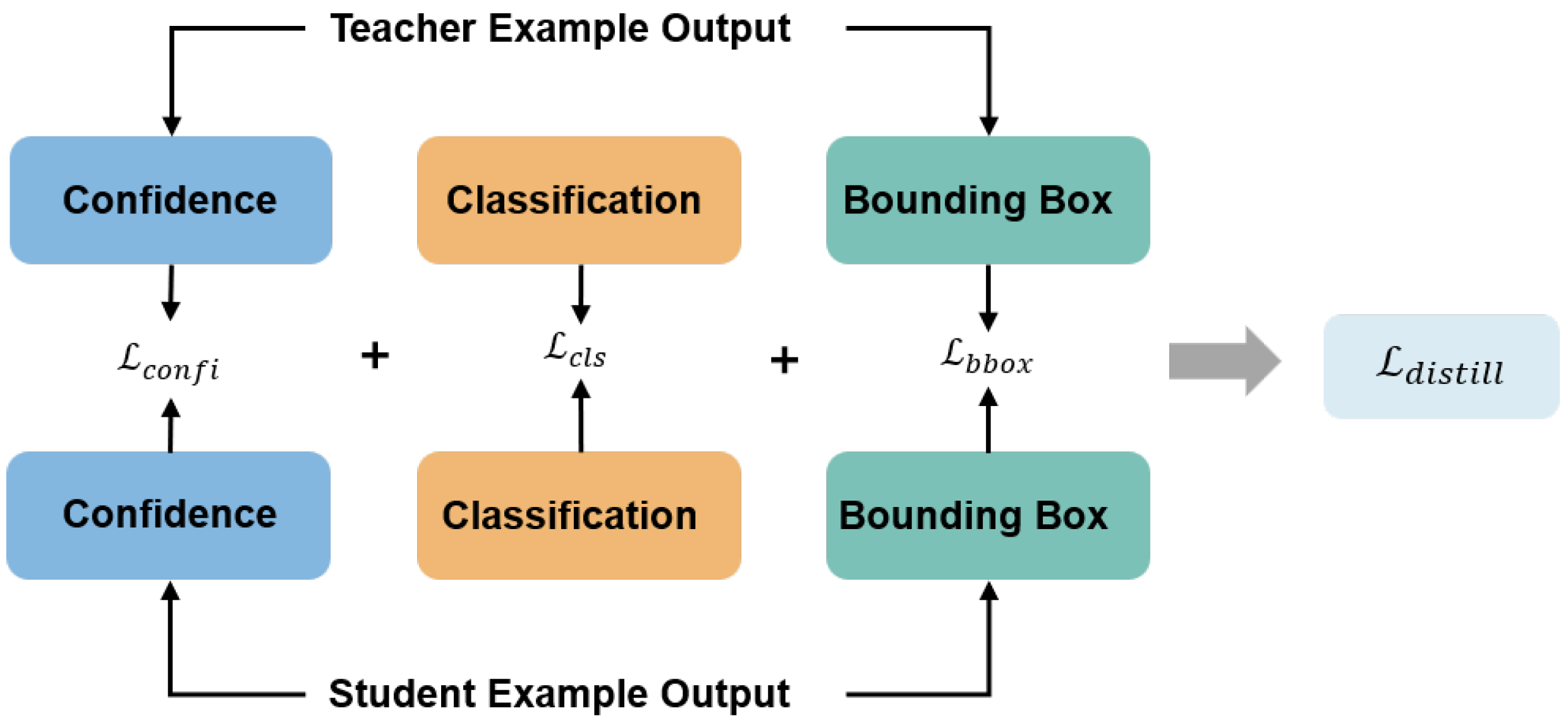
The detection model provides three types of information: confidence scores, classification probabilities, and bounding box predictions. In the standard training phase, each type of information serves a distinct optimization objective. Similarly, during the adversarial distillation phase, these three types of information play complementary roles in guiding the optimization of student patches. The components of the distillation loss are illustrated in Figure 4.

Specifically, the distillation of bounding box predictions helps student patches learn the optimal spatial directions for perturbation, ensuring maximal disruption to object localization. The distillation of classification probabilities informs the student patches which categories are more susceptible to attack, enabling more targeted adversarial effects. Finally, the distillation of confidence scores indicates which targets are easier to suppress, guiding the student patches to focus on the most vulnerable objects. The distillation loss ${\mathcal{L}}_{\mathrm{distill}}$ can be formulated as follows:

$${\mathcal{L}}_{\mathrm{distill}}={\lambda }_{\mathrm{conf}}·{\mathcal{L}}_{\mathrm{conf}}+{\lambda }_{\mathrm{cls}}·{\mathcal{L}}_{\mathrm{cls}}+{\lambda }_{\mathrm{bbox}}·{\mathcal{L}}_{\mathrm{bbox}}$$

(9)

Confidence Alignment Loss (${\mathcal{L}}_{\mathrm{conf}}$): The primary goal of the attack is to suppress object detections. This loss function is designed to efficiently transfer this capability from the teacher to the student:

$${\mathcal{L}}_{\mathrm{conf}}={\displaystyle \frac{1}{K}}\sum _{k=1}^K\left|\sqrt{c_k^T}-\sqrt{c_k^S}\right|+{\displaystyle \frac{1}{\left|\mathcal{U}\right|}}\sum _{j\in \mathcal{U}}{c}_j^S$$

(10)

The design of this loss is principled, efficiently handling both matched and unmatched detections—where a pair is considered matched if their IoU exceeds 0.2.

• For matched detection pairs (indexed by k), we innovatively minimize the L1 distance of the square root of the confidence scores. The core objective is to amplify the otherwise faint discrepancies between the teacher and student models in the low-confidence regime (e.g., 0.1 vs. 0.05). This “amplification effect” provides a clearer, more potent guidance signal for the student’s optimization.
• For unmatched boxes produced by the student patch ($\mathcal{U}$, indexed by j), where the teacher model detects nothing, the teacher provides an implicit “zero-confidence” target. In other words, the teacher’s silence is itself a form of guidance, indicating these detections should not exist. Therefore, the term ${\displaystyle \frac{1}{\left|\mathcal{U}\right|}}{\sum }_{j\in \mathcal{U}}{c}_j^S$ is not a simple regularization penalty, but a direct distillation loss against this implicit zero-target, essentially minimizing $|c_j^S-0|$.

Classification Alignment Loss (${\mathcal{L}}_{\mathrm{cls}}$): To ensure the student patch can induce the same misclassifications as the teacher, we align their probability distributions. Following standard practice in knowledge distillation, we employ the Kullback–Leibler (KL) divergence with a temperature scaling parameter $\tau =2.0$:

$${\mathcal{L}}_{\mathrm{cls}}={\tau }^2·\mathrm{KL}\left(\mathrm{softmax}\left({\displaystyle \frac{s^T}{\tau }}\right)\parallel \mathrm{softmax}\left({\displaystyle \frac{s^S}{\tau }}\right)\right)$$

(11)

The temperature $\tau$ softens the probability distributions, allowing the student model to learn from the nuanced class relationships captured by the teacher’s logits ($s_k^T$).

Bounding Box Alignment Loss (${\mathcal{L}}_{\mathrm{bbox}}$): The purpose of this loss is to extend the possible attack path. A bounding box predicted after the teacher’s attack represents a successful adversarial state, where the model’s internal features are likely severely corrupted. Thus, the true objective of ${\mathcal{L}}_{\mathrm{bbox}}$ is to guide the student’s predicted box locations toward the more adversarially potent directions established by the teacher, forcing it to predict in the most disruptive spatial state to study a more efficient attack knowledge. We employ the Generalized Intersection-over-Union (GIoU) loss to achieve this goal:

$${\mathcal{L}}_{\mathrm{bbox}}={\displaystyle \frac{1}{K}}\sum _{k=1}^K\left(1-\mathrm{GIoU}(b_k^T,b_k^S)\right)$$

(12)

Here, K is the number of matched bounding box pairs between the teacher and student outputs. For the k-th matched pair, $c^T,c^S$ are confidence scores, $s^T,s^S$ are classification logits, and $b^T,b^S$ are bounding box coordinates.

The final loss used to train the student patch integrates this distillation guidance with the fundamental attack objectives:

$${\mathcal{L}}_{\mathrm{stu}}=\alpha {\mathcal{L}}_d+\beta {\mathcal{L}}_{tv}+\eta {\mathcal{L}}_{sal}+\gamma {\mathcal{L}}_{\mathrm{distill}}$$

(13)

where $\alpha$, $\beta$, $\eta$, and $\gamma$ are weighting coefficients. By jointly optimizing these components, the student patch is guided to inherit a rich and multi-faceted adversarial capability from its teacher, thereby achieving high attack efficacy despite its compact size.

4. Experiment

4.1. Experimental Settings

4.1.1. Dataset

We evaluate the effectiveness of our proposed method on two remote sensing object detection datasets: the Military Aircraft Recognition 20 dataset (MAR20) [39] and the Remote Sensing Object Detection dataset (RSOD) [40]. The MAR20 dataset comprises 3842 high-resolution remote sensing images collected from 60 military airports worldwide via Google Earth. It includes 22,341 annotated instances across 20 distinct military aircraft models. The RSOD dataset, released by Wuhan University, contains 976 images annotated for four object categories: aircraft, oil tanks, playgrounds, and overpasses. Specifically, it includes 446 images with 4993 aircraft instances, 165 images with 1586 oil tanks, 189 images with 191 playgrounds, and 176 images with 180 overpasses. In our experiments, we focus primarily on attacking the aircraft class. All images are resized to a uniform resolution of $640\times 640$ pixels. Each dataset is split into training and validation sets using a 7:3 ratio. The object detection models are trained solely on the training set. During the adversarial attack phase, only the validation set is used for evaluation, ensuring no data leakage and a fair assessment of attack performance.

4.1.2. Evaluation Metrics

We evaluate attack performance using two complementary metrics: Attack Success Rate (ASR) and mean Average Precision (mAP). ASR measures the percentage of ground-truth objects that the detector fails to detect after the attack. It is defined as:

$$\mathrm{ASR}={\displaystyle \frac{N_{\mathrm{GT}}-N_{\mathrm{TP}}}{N_{\mathrm{GT}}}}\times 100\%$$

(14)

where $N_{\mathrm{GT}}$ is the total number of ground-truth objects and $N_{\mathrm{TP}}$ is the number of true positives detected on the attacked images. A higher ASR signifies a more effective attack.

mAP is the standard metric for evaluating object detection performance, calculated as the mean of Average Precision (AP) over all object categories. In our context, a lower mAP indicates a more significant degradation of the detector’s performance.

Together, these metrics provide a comprehensive assessment: ASR quantifies the attack’s success in making objects disappear, while mAP reflects the performance degradation on the objects that remain detectable.

4.1.3. Implementation Details

All experiments are conducted on a workstation equipped with an Intel i5-14600KF CPU, 32 GB of RAM, and an NVIDIA RTX 4080 GPU. The implementation is based on PyTorch 2.4.1 and CUDA 12.4. For training adversarial patches, the learning rate is set to $0.1$, and the maximum number of training epochs is fixed at 100. We use the Adam optimizer for gradient updates.

To enhance the visual naturalness and stealthiness of the generated adversarial patches, we incorporate the TV Loss and Sal Loss into the training objective. To enhance the robustness of adversarial patches under real-world lighting conditions, we apply a brightness adjustment during testing. During optimization, both the teacher and student patches are assigned identical weights for the TV and Sal losses to ensure appearance consistency and stable convergence. Meanwhile, the weights of other loss components are selectively adjusted according to different training objectives, such as detection suppression or knowledge distillation. The detailed parameter settings are provided in

Table 1. Loss function parameters configuration.

Parameters	Teacher Patches	Student Patches
Detect loss	1.0	0.3
TV loss	0.001	0.001
Sal loss	0.002	0.002
Distill loss	–	0.7

. A comprehensive summary of hyperparameters is provided in Appendix A.

During the training phase, the confidence threshold is set to 0.001 to ensure sufficient gradient feedback from low-confidence predictions. In the validation (attack) phase, we adopt a confidence threshold of 0.4 and an IoU threshold of 0.45 to determine true positive matches. These settings are consistent with common object detection protocols.

4.2. Comparisons to SOTA Methods

To evaluate the effectiveness of our proposed method, we conduct comprehensive comparative experiments between SDMPA, APPA, NAP, and the method proposed by Thys et al. The baseline adversarial attack methods, APPA and Thys et al., are selected based on the recent survey by Mei et al. [41], which summarizes the state-of-the-art adversarial patch attacks in RSI object detection. Furthermore, NAP is a representative of natural patch attacks. To obtain a fair comparison in the experiment, we constrained the total perturbation area at 9% of the target bounding box area.

For SDMPA, we deploy three perturbation patches per target object, with each patch occupying approximately 3% of the target area. For the baseline methods, APPA, NAP, and Thys et al., we configured them according to their original design to generate a single, larger patch that covers the same total perturbation area of 9% of the target. This setup allows us to evaluate the effectiveness of our method. The attack results are visualized in Figure 5.

The evaluations are performed on two widely used remote sensing object detection datasets, MAR20 and RSOD. Results are summarized in

Table 2. Performance Comparison of Patch Attack Methods on ASR and mAP for Five Detection Models.

Evaluation			Detection Models
Datasets	Metrics	Methods	YOLOv3	YOLOv5n	YOLOv5m	YOLOv5l	YOLOv8	Faster R-CNN
MAR20	ASR (%) ↑	Thys et al.	91.64	77.71	76.92	74.69	68.15	88.22
		APPA	88.94	82.29	83.58	72.31	74.55	91.95
		NAP	83.65	74.66	75.12	69.59	68.21	84.96
		SDMPA *	98.92	94.61	89.78	93.89	85.34	96.20
	mAP ↓	Thys et al.	0.494	0.473	0.681	0.594	0.641	0.273
		APPA	0.558	0.534	0.494	0.678	0.623	0.304
		NAP	0.578	0.584	0.523	0.629	0.682	0.382
		SDMPA *	0.232	0.269	0.273	0.318	0.404	0.151
RSOD	ASR (%) ↑	Thys et al.	78.32	66.09	68.07	73.24	63.38	78.80
		APPA	72.01	71.34	76.74	82.23	69.43	87.54
		NAP	74.46	63.21	73.89	78.34	67.66	76.65
		SDMPA *	93.23	88.30	85.40	82.37	79.83	93.32
	mAP ↓	Thys et al.	0.588	0.665	0.636	0.616	0.685	0.314
		APPA	0.553	0.531	0.504	0.609	0.749	0.373
		NAP	0.549	0.623	0.677	0.586	0.701	0.494
		SDMPA *	0.297	0.360	0.393	0.409	0.464	0.236

* Proposed methods; ↑: Higher is better; ↓: Lower is better.

.

As shown in Table 2, SDMPA consistently outperforms all baseline methods in terms of Attack Success Rate (ASR) across all models and datasets. For instance, on the MAR20 dataset, SDMPA achieves an ASR of 98.92% on YOLOv3, significantly higher than Thys et al. (91.64%), APPA (88.94%), and NAP (83.65%). The superiority is also evident against the more recent YOLOv8 model, where SDMPA achieves 85.34% ASR, far surpassing APPA (74.55%), NAP (68.21%), and Thys et al. (68.15%). Notably, when attacking the lightweight YOLOv5n model, SDMPA attains 94.61% ASR, demonstrating its robustness even on compact architectures. Similar trends are observed on other models, such as YOLOv5l and Faster R-CNN, where SDMPA maintains an ASR of above 93%, significantly outperforming prior approaches.

On the RSOD dataset, which contains smaller and more scattered objects, SDMPA remains superior. It achieves 93.23% ASR on YOLOv3 and 93.32% on Faster R-CNN, whereas APPA, Thys et al., and NAP show markedly lower performance, with ASRs often dropping below 80%. Against YOLOv8, SDMPA also shows a distinct advantage with an ASR of 79.83%, compared to baseline methods which fail to exceed 70%. This highlights SDMPA’s advantage in handling fine-grained, real-world scenarios, where object distributions are more complex.

In terms of detection quality degradation, SDMPA also achieves the lowest mean Average Precision (mAP) across nearly all settings, indicating its strong ability to suppress correct detections. For example, on the MAR20 dataset, SDMPA reduces the mAP on YOLOv5l to 0.318, a sharp decline compared to APPA (0.678), NAP (0.629), and Thys et al. (0.594). Similarly, on RSOD, the mAP on YOLOv5n drops to 0.360 under SDMPA, significantly lower than APPA (0.531), NAP (0.623), and Thys et al. (0.665). The degradation effect is consistent on the YOLOv8 model, where SDMPA records the lowest mAP on both MAR20 (0.404) and RSOD (0.464) datasets.

The experimental results demonstrate the effectiveness of SDMPA, which achieves a favorable balance between attack performance and patch size. This improvement is primarily attributed to its adaptive patch placement strategy and distillation-based generation mechanism. The individual contribution of each of these components will be analyzed in the following sections.

To assess the generalization ability of SDMPA, we evaluate its transferability across different detection models. Patches are generated on a source detector (e.g., YOLOv5l) and applied directly to other target models. In order to obtain fair results, we constrained the perturbation rate to 8%, and each target received 4 mini patches.

As shown in Table 3, SDMPA achieves strong black-box performance. For example, patches trained on YOLOv5l yield an ASR of 92.8% on YOLOv3 and 97.7% on Faster R-CNN, indicating effective cross-model transfer. Even lightweight models like YOLOv5n produce transferable patches, reaching 89.3% ASR on YOLOv5m.These results demonstrate that SDMPA generates compact patches with strong transferability, benefiting from its distillation-based optimization strategy.

4.3. Ablation Study

To further validate the contributions of the proposed modules, this study conducted an ablation experiment, and the results are summarized in Table 4. The target model is YOLOv5L, and the dataset used is the MAR20 military aircraft remote sensing image dataset. The experiments in Table 2 are designed to evaluate the effectiveness of the ASAP and DMPG modules.

Table 3. Cross-model transferability of SDMPA. Diagonal entries (in bold) are white-box attacks.

Source	Metrics	YOLOv3	YOLOv5n	YOLOv5m	YOLOv5l	YOLOv8	Faster R-CNN
YOLOv3	ASR (%)	91.41	88.16	91.63	89.75	82.50	91.98
	mAP	0.270	0.290	0.261	0.358	0.380	0.213
YOLOv5n	ASR (%)	94.61	90.76	89.38	85.68	78.20	91.53
	mAP	0.233	0.338	0.208	0.326	0.420	0.220
YOLOv5m	ASR (%)	91.67	90.42	93.24	80.54	81.60	95.87
	mAP	0.204	0.320	0.250	0.294	0.390	0.215
YOLOv5l	ASR (%)	92.85	91.87	93.68	89.23	84.70	97.78
	mAP	0.161	0.318	0.254	0.278	0.360	0.213
YOLOv8	ASR (%)	86.40	82.30	85.50	81.20	82.34	92.60
	mAP	0.280	0.350	0.290	0.320	0.434	0.240
Faster R-CNN	ASR (%)	83.52	86.88	83.54	76.05	72.80	95.83
	mAP	0.269	0.471	0.349	0.424	0.480	0.279

Table 3. Cross-model transferability of SDMPA. Diagonal entries (in bold) are white-box attacks.

Source	Metrics	YOLOv3	YOLOv5n	YOLOv5m	YOLOv5l	YOLOv8	Faster R-CNN
YOLOv3	ASR (%)	91.41	88.16	91.63	89.75	82.50	91.98
	mAP	0.270	0.290	0.261	0.358	0.380	0.213
YOLOv5n	ASR (%)	94.61	90.76	89.38	85.68	78.20	91.53
	mAP	0.233	0.338	0.208	0.326	0.420	0.220
YOLOv5m	ASR (%)	91.67	90.42	93.24	80.54	81.60	95.87
	mAP	0.204	0.320	0.250	0.294	0.390	0.215
YOLOv5l	ASR (%)	92.85	91.87	93.68	89.23	84.70	97.78
	mAP	0.161	0.318	0.254	0.278	0.360	0.213
YOLOv8	ASR (%)	86.40	82.30	85.50	81.20	82.34	92.60
	mAP	0.280	0.350	0.290	0.320	0.434	0.240
Faster R-CNN	ASR (%)	83.52	86.88	83.54	76.05	72.80	95.83
	mAP	0.269	0.471	0.349	0.424	0.480	0.279

Table 4. Ablation Study Results for ASAP and DMPG Modules.

ASAP	DMPG	Metric	Patch Number per Target
			1	2	3	4	5
0	0	ASR (%)	61.0	65.9	63.5	60.9	65.0
		mAP	0.768	0.709	0.741	0.750	0.751
0	1	ASR (%)	63.6	67.5	70.1	64.6	67.3
		mAP	0.742	0.693	0.679	0.735	0.757
1	0	ASR (%)	72.1	78.6	80.1	77.9	78.4
		mAP	0.681	0.608	0.550	0.568	0.579
1	1	ASR (%)	74.5	83.3	82.5	86.5	83.7
		mAP	0.662	0.517	0.507	0.494	0.528

Table 4. Ablation Study Results for ASAP and DMPG Modules.

ASAP	DMPG	Metric	Patch Number per Target
			1	2	3	4	5
0	0	ASR (%)	61.0	65.9	63.5	60.9	65.0
		mAP	0.768	0.709	0.741	0.750	0.751
0	1	ASR (%)	63.6	67.5	70.1	64.6	67.3
		mAP	0.742	0.693	0.679	0.735	0.757
1	0	ASR (%)	72.1	78.6	80.1	77.9	78.4
		mAP	0.681	0.608	0.550	0.568	0.579
1	1	ASR (%)	74.5	83.3	82.5	86.5	83.7
		mAP	0.662	0.517	0.507	0.494	0.528

In addition, to assess the effectiveness of using multiple patches, we constrained the total perturbation rate to 5% per target and compared the attack results with different numbers of patches. For example, when the number of patches is one, the patch size is 5%; when the number of patches is five, each patch size is 1% of the target.

Table 4 summarizes the ablation results for the proposed ASAP and DMPG modules under varying patch counts. Several insights can be drawn from the results:

• Effect of Multi-Patch Strategy: As observed in the baseline setting (ASAP = 0, DMPG = 0), increasing the number of patches from one to five leads a rise in ASR from 61.0% to 65.0%. When both ASAP and DMPG are enabled (bottom row), ASR increases more significantly—from 74.5% with a single patch to 86.5% with four patches. This demonstrates the effectiveness of the multi-patch strategy when guided by adaptive placement and learning mechanisms.
• Effect of the ASAP Module: When comparing settings with ASAP = 0 and ASAP = 1 (with DMPG fixed), notable improvements are observed. For instance, under three patches, ASR increases from 63.5% to 80.1%, and mAP decreases from 0.741 to 0.550. This indicates that adaptive patch placement, guided by attention and gradient information, substantially enhances attack performance.
• Effect of the DMPG Module: Comparing the rows with and without DMPG under the same ASAP setting reveals the positive impact of DMPG. For example, with ASAP enabled and three patches applied, incorporating DMPG boosts ASR from 80.1% to 82.5%, while further reducing mAP from 0.550 to 0.507. These results confirm that DMPG improves attack strength by distilling patch effectiveness from a larger teacher patch.

An interesting phenomenon was observed in the configuration without the DMPG module, while the ASR generally increased when moving from one to three patches, it unexpectedly decreased when the patch count was raised to four.

A plausible explanation for this degradation is that as the number of patches increases, the dimensionality of the optimization space grows substantially. We hypothesize that without the regularizing guidance provided by a teacher model, the optimization process becomes easier to get stuck in a local best optimization. This phenomenon highlights the challenge of naive multi-patch attack strategies.

In stark contrast, the full SDMPA framework (with DMPG enabled) demonstrated improvement in performance as more patches were added. This suggests that the knowledge distillation mechanism serves as an effective guide for the optimization process, helping to navigate the complex search space and mitigate the instability observed in the baseline, thereby ensuring that additional patches contribute positively to the overall attack efficacy.

4.4. Discussions

4.4.1. Effectiveness of Multi-Patch Strategy

To further analyze the effectiveness of the multi-patch strategy in adversarial attacks, we investigated the impact of different placement strategies on attack performance. For this experiment, the DMPG module was disabled for all methods except for the final one (the full SDMPA framework). To isolate the effect of placement, we used identical base patches created by directly scaling a single APPA patch and only varied their spatial locations.

We established a comprehensive set of comparative experiments. First, we set a single-patch baseline using a conventional attack method. For the multi-patch attacks, we tested four distinct placement strategies: random placement, placement guided only by the Explainable Map (EM), placement guided only by the Adversarial Map (AM), and placement guided by the complete ASAP module, which fuses both EM and AM. Finally, to demonstrate the superiority of our complete attack framework, we included the performance of the full SDMPA for comparison. The experiment results are illustrated in Figure 6.

At a 9% total perturbation rate, the random placement strategy achieved an Attack Success Rate (ASR) of only 67.61%, which is significantly lower than the single-patch baseline’s 82.29%. This indicates that blindly increasing the number of patches does not improve the attack success rate. On the contrary, guiding the placement using feature maps that represent the model’s attention under different conditions enhances attack performance, demonstrating that the effectiveness of distributed perturbations relies on a valid placement strategy.

At the same 9% perturbation rate, using only EM or AM yielded ASRs of 86.1% and 79.3%, respectively. When fused, the complete ASAP module (EM+AM) further boosted the ASR to 88.2%. This clearly shows that the model’s explainable features (EM) and adversarial sensitivities (AM) contain complementary information. Their fusion allows for a more precise localization of the target’s vulnerable regions, leading to a stronger attack than either strategy alone.

The complete SDMPA framework achieves optimal attack performance. Under all tested perturbation levels, the full SDMPA method consistently demonstrated the best results. This confirms that our proposed framework, by combining the multi-patch strategy with knowledge distillation, effectively enhances overall attack performance.

4.4.2. Effect of Distillation

We designed an experiment to explore the contribution of each patch. In this experiment, we fixed the size of each individual adversarial patch to 2% of the target object size and varied the total number of patches, thereby controlling the overall perturbation range from 2% to 10%. The corresponding Attack Success Rate (ASR) and mean Average Precision (mAP) are shown in Figure 7.

As illustrated in Figure 7, the ASR and mAP curves exhibit that the attack performance does not increase linearly with the number of patches. Instead, as the search space for adversarial perturbations expands, the improvement in adversarial effectiveness follows a diminishing return pattern. This phenomenon suggests that simply increasing the number of patches leads to less significant performance gains after a certain threshold, likely due to overlapping perturbations and redundant interference.

Furthermore, by introducing Knowledge Distillation (KD) into the multi-patch strategy, the curves for both ASR and mAP show a more gradual decline compared to the non-distilled baseline. This indicates that knowledge distillation plays a crucial role in guiding the optimization process, helping the model focus on more effective regions and preventing performance degradation as additional patches are added. The distillation mechanism reduces the adverse effects caused by excessive patching, thus improving the overall attack success and preserving detection accuracy better than without distillation.

Additionally, we explored the impact of teacher patch size on the distillation performance of student patches. The size of the teacher patch directly influences the amount of adversarial information transferred to the student model. As shown in Figure 8, the perturbation introduced by the teacher patch varies based on its size, which in turn affects the student model’s ability to learn adversarial patterns effectively.

The optimal teacher patch size balances the extent of perturbation with the specificity needed in the attack. In this study, we found that a teacher-to-student patch size ratio in the range of 1.75 to 2.75 yielded the best results in guiding the student model. Specifically, the highest mAP was observed at a ratio of 2.0, while the highest ASR was achieved at 2.25. These findings suggest that for multi-patch adversarial attacks, both the number of patches and the teacher patch size are critical factors for optimizing the distillation performance. This indicates that not only the number of patches but also the teacher patch size, plays a crucial role in determining the effectiveness of the distillation process.

When the teacher patch size is too small, the adversarial strength is insufficient, resulting in limited guidance for the student model. Conversely, when the teacher patch size is too large, the dimensional disparity between the teacher patch’s high-dimensional space and the student patch’s space becomes too significant, causing the guidance to lose its effectiveness. Therefore, to achieve optimal distillation performance, it is essential to control the ratio between the teacher patch and the student patch sizes.

To investigate the performance of each component within our proposed distillation loss, we conducted a comprehensive ablation study by testing all possible combinations of the three loss terms. The results are summarized in

Table 5. Ablation study on the components of the distillation loss.

Method	ASR (%)	mAP	Method	ASR (%)	mAP
Non-distill (base)	81.8	0.477	Bbox	83.5	0.458
Confidence	84.8	0.448	Bbox + Confi	84.6	0.437
Confidence + Cls	88.0	0.428	Bbox + Confi + Cls	84.8	0.453
Cls	87.5	0.436	Bbox +Cls	86.8	0.438

, from which we draw several key observations.

First, the introduction of any single distillation component significantly outperforms the non-distillation baseline (ASR 81.8%, mAP 0.477). Specifically, the Classification Loss (cls) alone provides the most substantial improvement among the individual components, achieving an ASR of 87.5% and reducing the mAP to 0.436. This indicates that aligning the classification probability distributions is a powerful mechanism for transferring adversarial knowledge, which may also be attributed to the superior effectiveness of knowledge transfer through the classification loss.

Second, when combining two components, the confi+cls configuration demonstrates superior performance, achieving the highest ASR of 88.0% and the lowest mAP of 0.428. This synergistic effect highlights that guiding the student patch to simultaneously suppress object confidence and mimic the teacher’s misclassification behavior is the most effective strategy.

Interestingly, the inclusion of the bounding box loss (bbox) does not consistently enhance attack performance and, in some cases, even degrades it. For instance, the combination of bbox+confi+cls yields a lower ASR (84.8%) compared to the confi+cls combination. This phenomenon suggests that while aligning bounding box predictions is intuitively plausible, it may introduce conflicting optimization objectives or noisy gradients within our framework, ultimately failing to effectively enhance the distillation process for attack generation.

The inclusion of the bounding box loss ($L_{bbox}$) does not consistently enhance attack performance, primarily due to a fundamental conflict in its optimization objective. The ultimate goal of the attack is detection suppression—eliminating the bounding box entirely. However, $L_{bbox}$ inherently guides the student patch toward a suboptimal state of mimicking a teacher’s damaged detection, an unstable and noisy signal. Unlike the classification loss ($L_{cls}$), which provides a clear, semantic-level directive for feature disruption, $L_{bbox}$ only offers a vague spatial assessment without a clear optimization path. Consequently, the combination of confidence ($L_{conf}$) and classification ($L_{cls}$) alignment is more effective, as both synergistically target the core task with potent and unambiguous guidance.

4.4.3. Physical Experiment

To evaluate the deployability and physical-world effectiveness of the SDMPA framework, we conducted a set of real-world experiments involving printed adversarial patches. The objective was to assess whether adversarial patches generated digitally could retain their attack efficacy when physically printed, attached to remote sensing images, and re-captured via camera for inference by an object detector.

The experimental setup was as follows. Our test target was a 1:200 scale model of a C-17 transport aircraft (real-world dimensions: 53.04 m length, 51.81 m wingspan), featuring a length of 26.5 cm and a wingspan of 25.9 cm. The adversarial patches were printed at a resolution of 600 DPI to ensure high fidelity. The large single patch used for baseline comparison measured 7 cm × 7 cm, while the SDMPA mini-patches were 3 cm × 3 cm. To translate the digitally optimized patterns to their physical print dimensions, bilinear interpolation was employed for scaling. For the recapture process, a Redmi K70 Ultra with Sony IMX906 camera was used at a fixed distance of 3 m from the model.

The attack results against the YOLOv5L detector are presented in Figure 9. We evaluated six scenarios to benchmark our method against baselines and assess its rotational robustness. The results demonstrate that SDMPA-generated mini-patches exhibit superior real-world adversarial performance. In contrast, both the traditional large-patch method and a naive resizing of this patch placed at ASAP-identified locations failed to suppress detection, yielding confidence scores of 0.52 and 0.32, respectively. Notably, the SDMPA patches not only successfully evaded detection but also maintained their effectiveness under a $-{45}^{\circ }$ rotation, showcasing a degree of robustness to viewpoint variations.

Furthermore, this experiment highlights the significant practical advantages of the multi-patch strategy for deployment on large-scale or irregularly shaped targets. Using the C-17 as an example, a proportionally scaled single large patch would require an impractically massive 14 m × 14 m pattern on a real aircraft. In contrast, our method utilizes multiple, far more manageable 6 m × 6 m patches. This size reduction offers two key benefits: enhanced convenience of physical application and greater flexibility in deployment. A vast 14 m × 14 m area might offer only a single placement option on the aircraft’s fuselage—if any. Conversely, multiple smaller patches can be flexibly adapted to various surfaces like the wings, tail, and fuselage, conforming better to the target’s complex geometry.

In summary, the physical experiment confirms that the SDMPA framework not only achieves success in the digital domain but also possesses tangible physical-world applicability. Its robustness to rotation suggests strong potential for real-world deployment in aerial scenarios involving varying angles. Future work could integrate additional physical constraints, such as lighting variations and motion blur, to further enhance its generalization and reliability.

5. Conclusions

In this paper, we propose SDMPA, a novel framework for multi-mini-patch attacks for remote sensing object detection. Unlike traditional adversarial patch methods that rely on a single large patch, our approach strategically places multiple compact patches using the Adaptive Sensitivity-Aware Positioning (ASAP) module and enhances their adversarial potency through knowledge distillation in the Distillation-based Mini-Patch Generation (DMPG) module. Extensive experiments on the MAR20 and RSOD datasets demonstrate that SDMPA significantly improves the attack success rate (ASR) and reduces detection performance (mAP) while maintaining minimal patch size, while these results are promising, future work could further enhance the framework. Key directions include improving the keypoint localization accuracy in ASAP and exploring stronger feature associations among student patches within DMPG.