Radio Propagation Characteristics in Several Application Scenarios at 285 GHz Terahertz Band

Abstract

In this paper, we have derived R.M.S. delay spread characteristics and models according to the influence of antenna beam width in the mobile kiosk data download environment, the inter-rack communication environment in the data center, the intra-device communication environment, and the experimental laboratory measurement environment scenario in the 275 GHz to 295 GHz bands. The measurement system used in this paper used a vector network analyzer and a frequency expander to derive the statistical characteristics of terahertz frequency band signals, and used antennas with different beamwidths for measurement. It is confirmed that the distribution of delay spread varies depending on the beam width of the antenna used for measurement and the type of measurement scenario.

1. Introduction

The rapid proliferation of data-centric services and the emergence of sixth-generation (6G) networks are driving unprecedented demand for ultra-high-speed wireless communication. According to Shannon’s capacity theorem, data rates can be improved by either increasing the signal-to-noise ratio (SNR) or expanding the available bandwidth. Given the practical limitations in enhancing signal quality, exploiting higher frequency bands has become a pivotal strategy for next-generation wireless systems. The terahertz (THz) band, spanning 275 GHz to 3 THz, offers immense bandwidth potential, enabling multi-gigabit-per-second data rates over short distances.

THz waves exhibit unique physical properties, including high directivity, low diffraction, and partial penetration through dielectric materials. These characteristics position the THz band as a promising candidate for applications such as kiosk-based data services, inter-chip and intra-device communication, and high-speed data center interconnects [1].

Historically, the practical deployment of THz systems has been hindered by hardware limitations and severe propagation losses. However, recent advancements in THz sources and detectors have reignited research interest. Several studies have highlighted the significance of accurate channel characterization and delay spread modeling in this frequency range. For instance, Rappaport et al. [2] and Han et al. [3] emphasized the role of multipath effects in short-range THz links, while Jornet and Akyildiz [4] proposed foundational channel models. Further contributions by Sarieddeen et al. [5] and Samimi and Rappaport [6] explored signal processing and statistical modeling techniques for THz propagation. Complementary surveys, such as that by Abbasi et al. [1], also summarized application domains and standardization progress for THz communication systems.

Standardization efforts have also progressed. The ITU-R extended the upper frequency limit of its indoor channel model to 450 GHz in Recommendation P.1238-11 [7], and WRC-19 formally allocated the 275–450 GHz band for active services. Regulatory and modeling perspectives have been discussed by Kürner and Priebe [8], while a recent study by Tekbıyık and Uysal [9] provided detailed insights into indoor THz measurement methodologies and modeling directions. From a broader perspective, millimeter-wave (mmWave) systems, which serve as a precursor to THz communication, have also demonstrated the viability of high-frequency mobile broadband, as noted by Pi and Khan [10].

This paper contributes to this evolving field by presenting a comprehensive analysis of R.M.S. delay spread in the 275–295 GHz band across four practical deployment scenarios: kiosk-based data downloading, inter-rack communication in data centers, intra-device communication, and controlled laboratory experiments. Measurements were conducted using a vector network analyzer with frequency extenders and horn antennas of 10°, 30°, and 60° beamwidths to evaluate the effect of antenna directivity. From the resulting power delay profiles (PDPs), statistical models of R.M.S. delay spread were derived as functions of received power. The findings provide valuable insights into channel behavior and offer design guidelines for future low-THz wireless systems.

2. Measurement Campaign

2.1. Measurement Setup

Channel measurements were conducted in the 275–295 GHz frequency band using a Keysight N5227B vector network analyzer (VNA) combined with VDI’s WR 3.4 frequency extenders. The measurement system supports a total bandwidth of 20 GHz with a frequency step size of 16.67 MHz, resulting in 1201 frequency points per sweep. The intermediate frequency (IF) filter bandwidth was set to 10 kHz. This configuration provides a time-domain resolution of 0.05 ns and a maximum delay range of 30 ns. Figure 1 illustrates the overall measurement setup, including the transmitter and receiver devices used in the experiment. The VNA and frequency extender modules are mounted on height-adjustable frames to allow flexible antenna positioning. The transmitter can be manually rotated both horizontally and vertically, while the receiver is placed on a motorized linear stage for precise spatial scanning. The transmitter system consists of a horizontally fixed VNA and frequency extender mounted on a mechanical structure that allows vertical height adjustment and manual rotation in both horizontal (0° to 180°) and vertical (−70° to 0° down-tilt) directions. The transmitting antenna can be positioned at heights between 0.8 m and 2.0 m. The receiver system is configured similarly, with a VNA and extender installed on a vertically adjustable mount. The receiver is mounted on a motorized linear stage with a movement range of 1 m and a resolution of 0.5 mm to 1 mm. Additionally, a vertical translation device (range: 800 mm to 1300 mm) and a 360° azimuth rotator with 1° resolution are controlled by custom software to ensure precise positioning. Horn antennas with three different beamwidths—10° (22 dBi gain), 30° (14 dBi), and 60° (7 dBi)—were used for both transmission and reception. All antennas are linearly polarized in the vertical direction and employed in matched pairs (i.e., the same beamwidth at both Tx and Rx). The key measurement parameters are summarized in Table 1.

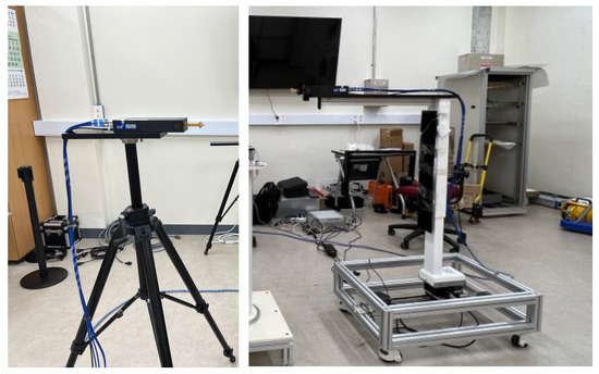
Figure 1. Transmitter and receiver device. (left: transmitter, right: receiver).

Table 1. Measurement parameters.

Parameters	Value	Remark
Frequency	275~295 GHz	Center: 285 GHz
Bandwidth	20 GHz
IF Filter Bandwidth	10 kHz
Frequency Points	1201
Frequency Step Size	16.67 MHz
Time Domain Resolution	0.05 ns	1/20 GHz
Time Domain Range	30 ns	1200 × 0.05/2

2.2. Kiosk Measurement Scenario

The kiosk data downloading scenario was designed to emulate a mobile service environment where users interact with a polyethylene terephthalate (PET) panel, typically 2.3 mm thick. In this experiment, the distance between the transmitter and the panel was fixed, while the distance between the panel and the receiver was varied. Three horn antennas with beamwidths of 10°, 30°, and 60° were used for both transmission and reception, maintaining matched polarization and gain characteristics. To minimize internal reflections, radio wave absorbers were attached inside the kiosk enclosure. The overall measurement configuration for this scenario is shown in Figure 2. Three specific sub-scenarios were examined to analyze delay spread characteristics under different geometric conditions.

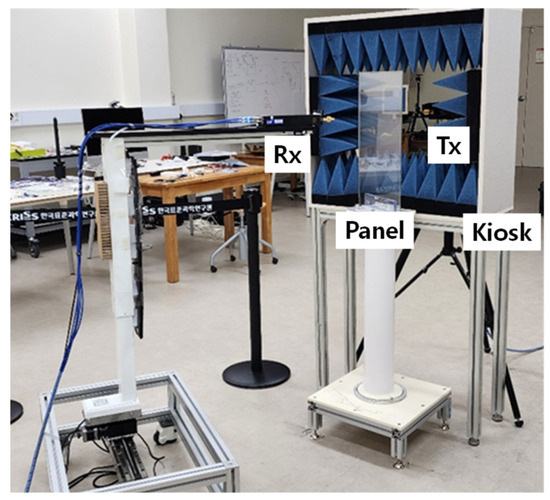
Figure 2. Measurement environment for the kiosk data downloading system.

Scenario 1 (Figure 3): The transmitter, receiver, and kiosk panel are arranged in parallel. The transmitter is fixed, while the receiver moves along two predefined paths:

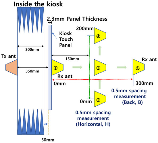
Figure 3. Top view of measurement Scenario #1.

Path A (①→②→③)—movement away from the panel in the backward direction, up to 300 mm;

Path B (⑤→②→④)—vertical movement of ±100 mm around a position 150 mm from the panel.

Measurements were taken at 5 mm intervals along both paths.

Scenario 2 (Figure 4): The transmitter and receiver remain parallel, but the kiosk panel is tilted forward by 30°, increasing the transmitter-to-panel distance to 365 mm. The receiver movement and measurement intervals are identical to those in Scenario 1.

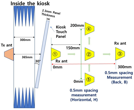
Figure 4. Top view of measurement Scenario #2.

Scenario 3 (Figure 5): Both the kiosk panel and the receiver are tilted forward by 30°, maintaining the 365 mm distance between the panel and transmitter as in Scenario 2. The receiver movement patterns and sampling intervals are the same as in the previous scenarios. These three configurations enable a comprehensive analysis of R.M.S. delay spread variations as a function of the antenna beamwidth and geometric alignment in realistic kiosk service environments.

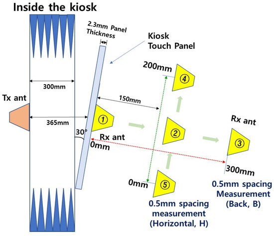
Figure 5. Top view of measurement Scenario #3.

2.3. Rack Measurement Scenario

Experimental measurements were carried out to evaluate inter-rack communication performance in a representative data center environment. In this scenario, the transmitter was fixed at a constant distance from a small wired mesh panel with a thickness of 0.3 mm, while the distance between the panel and the receiver was systematically varied. Horn antennas with beamwidths of 30° and 60° were employed at both the transmitter and receiver sides, and matched antenna pairs were used to ensure consistent measurement conditions. The measurement setup is illustrated in Figure 6 and Figure 7. To analyze spatial variations in received signal characteristics within the rack, the receiver antenna was translated along two orthogonal directions inside the rack structure, denoted as the “back” and “horizontal” directions. Figure 8 provides a top-down view of the setup shown in Figure 6, offering a planar representation of the receiver’s motion path relative to the fixed transmitter. Along each direction, measurements were acquired at 3 mm intervals over a linear track. After completing a measurement sweep at one vertical level, the receiver was repositioned vertically, and the same process was repeated at the new height, as depicted in Figure 8. To replicate realistic inter-rack deployment conditions, common obstructions such as LAN cables and small wired mesh panels were deliberately introduced inside the rack. These obstructions emulate the impact of practical environmental clutter on propagation characteristics and are critical in understanding delay spread behavior in data center scenarios.

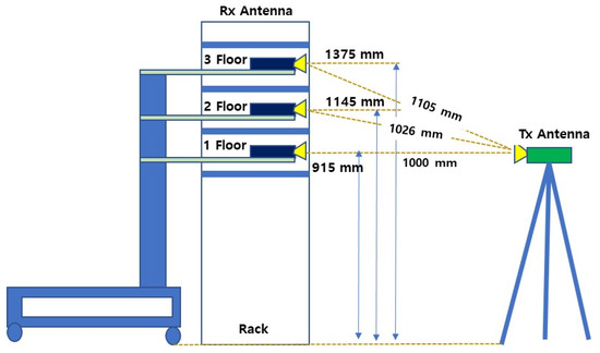
Figure 6. Rack measurement system configuration.

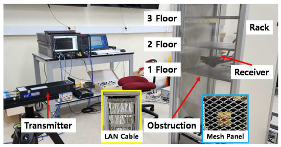
Figure 7. Rack measurement environment.

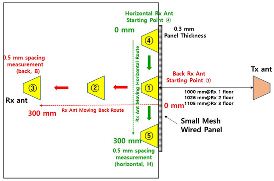
Figure 8. Rack measurement system plain figure.

2.4. Inter-Device Measurement Scenario

To construct the intra-device measurement environment, two types of desktop computer cases—one large and one small—were selected, with certain internal components intentionally left intact to emulate realistic internal structures. Line-of-sight (LoS) propagation was maintained between the transmitter and receiver antennas to ensure consistency in the measurement conditions. Figure 9a,b depict the exterior of the large and small PC cases, respectively, while Figure 9c presents the dimensional specifications of each case. The specific port holes used for antenna placement, including their relative positions and exact circuit board locations, are illustrated in Figure 9d. Multiple propagation paths within each case were defined and are shown in Figure 10. Among them, Figure 10a,c represent straight-line paths, while Figure 10b shows a 90-degree bent path and Figure 10d depicts a slanted path. The separation distances between the transmitter and receiver antennas for all paths of the big case and small case are summarized in Table 2. For each measurement, only one antenna port was opened at a time, while all remaining ports were sealed using metallic tape to minimize unwanted signal leakage, as illustrated in Figure 11 and Figure 12. After performing vector network analyzer (VNA) calibration, reference power levels were established to normalize the received signal power. Delay spread characteristics were then extracted from the measured power delay profiles (PDPs), and the distances used for these analyses of the tiny case are listed in Table 3.

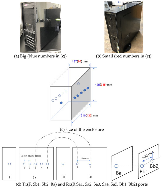
Figure 9. Intra-device environment.

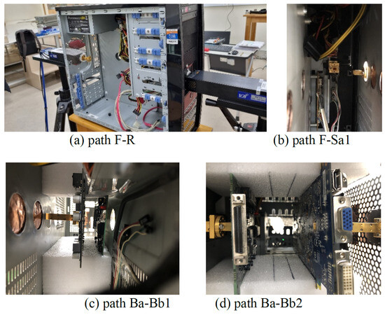
Figure 10. Photos of radio paths.

Table 2. The shortest distances of all radio paths.

Tx-Rx Path (mm)	F-R	F-Sa1	F-Sa2	F-Sa3	F-Sa4	F-Sa5	Sb1-Sa1	-
Big	375	110	158	207	256	303	125	-
Small	310	65	111	158	208	257	123	-
Tx-Rx Path (mm)	Sb1-Sa2	Sb1-Sa3	Sb2-Sa1	Sb2-Sa2	Sb2-Sa3	Sb2-Sa4	Sb2-Sa5	-
Big	90	75	214	168	125	90	75	-
Small	87	65	212	166	123	87	71	-
Tx-Rx Path (mm)	Ba-Bb1				Ba-Bb2
Big	68	88	108	128	121	133	147	162
Small	28	48	68	-	104	111	121	-

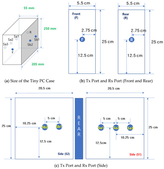
Figure 11. Tiny case size.

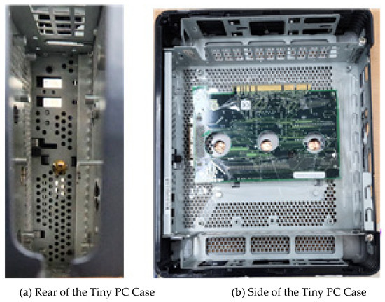
Figure 12. Intra-device measurement photo.

Table 3. The shortest distances (mm) between Tx and Rx inside the PC case (tiny). Unit: mm.

Tx-Rx Path (mm)	F-R	F-Sa1	F-Sa2	F-Sa3	Sb1-Sa1
Tiny Case	195	107	91.6	81.1	45
Tx-Rx Path (mm)	Sb1-Sa2	Sb1-Sa3	Sb2-Sa1	Sb2-Sa2	Sb2-Sa3
Tiny Case	60.4	74.5	60.4	45	60.4

2.5. Experiment Laboratory Measurement Scenario

Experimental measurements were carried out in a confined laboratory space measuring 11 m × 17 m to investigate delay characteristics under controlled indoor conditions. All transmit antennas were installed at a height of 2 m and tilted downward by 30°, while receive antennas were positioned at a height of 1.5 m. The distance between the transmitter and receiver was varied from 1.5 m to 4.5 m in 0.5 m increments, resulting in corresponding spatial separations ranging from 1.7 m to 5.0 m due to the angular tilt. For all measurements in this scenario, both the transmitting and receiving antennas were configured with a beamwidth of 60°. To capture the angular diversity of incoming signals, the receiver antenna was rotated in 5° steps through a full 360° azimuthal sweep at each position. Figure 13 illustrates the side and top views of the antenna arrangements and movement trajectories. Among the measured links, the shortest separation occurred between transmitter location 1 and receiver location 1, while the longest was observed between transmitter location 2 and receiver location 7. Figure 14 shows photographs of the actual measurement setup, including equipment placement at the designated transmitter locations within the laboratory environment.

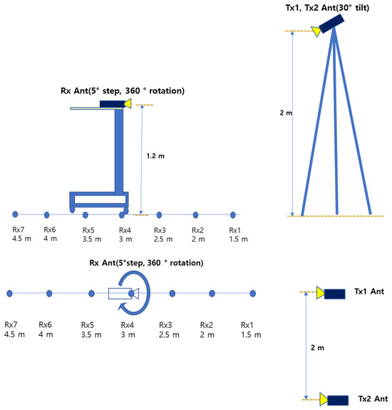
Figure 13. Laboratory measurement side and top views.

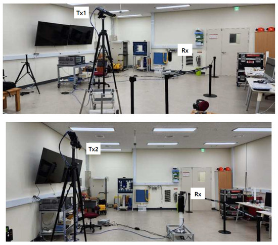
Figure 14. Picture of measurements at transmitter locations 1 (upper) and 2 (lower).

2.6. Technical Requirements and Applications of Scenarios

The four measurement scenarios investigated in this study represent practical deployment cases envisioned for future low-THz wireless communication systems. Each scenario is associated with specific technical requirements and application targets, as summarized below.

Kiosk Data Downloading: Intended for high-speed, short-range access services such as interactive content delivery and AR/VR applications. The technical requirements emphasize ultra-high throughput (>10 Gbps) with stable connectivity over distances of a few tens of centimeters, while accounting for user–panel interactions.

Inter-rack Communication in Data Centers: Targeted for low-latency (<1 μs) and high-reliability interconnections between racks. This scenario supports applications such as cable-free data center interconnects and rack backplane replacement, where environmental clutter from cables and panels must be carefully considered.

Intra-device Communication: Designed for chip-to-chip and board-to-board communication within electronic devices. The key requirement is compact integration with minimal delay spread to avoid inter-symbol interference (ISI), enabling multi-Gbps wireless bus replacement inside confined device enclosures.

Experimental Laboratory Environment: Provides a controlled reference scenario for evaluating THz propagation fundamentals, such as path loss exponents and multipath dispersion. This environment supports the development of baseline models and serves as a benchmark for validating measurements in real-world deployment cases.

2.7. Comparative Summary of Environmental Characteristics

To improve clarity, Table 4 summarizes the common and distinct features of the four measurement scenarios. The table highlights the intended applications, geometric conditions, antenna configurations, and environmental characteristics of each scenario, thereby enhancing the comprehensiveness of the experimental setup.

Table 4. Comparative summary table of the measurement scenarios.

Scenario	Measurement Distance	Obstructions	Antenna Beamwidths	Environment Type	Key Features
Kiosk-based data downloading	0.1–0.3 m	PET panel (2.3 mm thick), with/without tilt	10°, 30°, 60°	Semi-enclosed	Short-range, panel penetration/reflection effects
Inter-rack communication (data center)	~0.3–1.0 m	LAN cables, small mesh panel, none	30°, 60°	Semi-enclosed rack space	Multipath from in-rack obstructions
Intra-device communication	0.03–0.38 m (varies by path)	Internal components, PCB structures	5°, 60°	Fully enclosed	Strong multipath in confined space
Experimental laboratory environment	1.5–4.5 m	None (controlled environment)	60°	Open indoor lab	Reference channel for model validation

3. Measurement Results

3.1. Kiosk

In this section, the measurement results for all scenarios conducted in the kiosk data downloading environment are analyzed in terms of the root-mean-square (R.M.S.) delay spread. Figure 15 illustrates the variation in relative received power as a function of the distance between the transmitting and receiving antennas. While the absolute values along the y-axis differ depending on the specific measurement scenario, a general trend of decreasing received power with increasing distance is observed on a large-scale basis. However, on a finer scale, localized increases in received power are also detected at certain distances, indicating the presence of small-scale fading phenomena. These fluctuations are likely caused by multipath reflections and constructive interference, which become more pronounced as the distance between the antennas increases. The superposition of these effects highlights the importance of accounting for both large- and small-scale propagation characteristics in analyzing R.M.S. delay spread within the kiosk-based service environment.

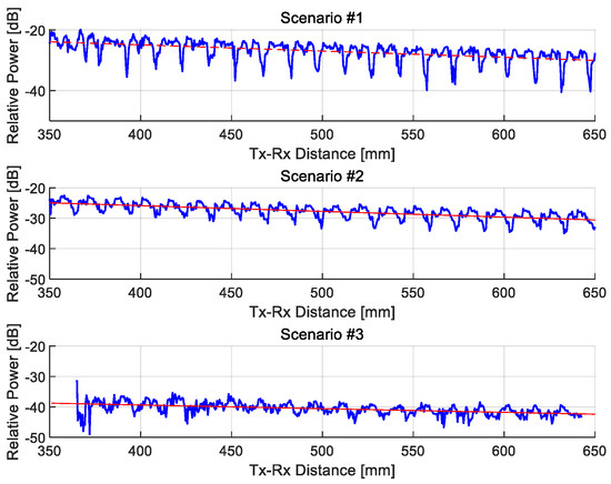
Figure 15. Relative received power according to the Tx-Rx distance in Scenarios #1, 2, and 3. (blue line: actual measurements, red line: trend line).

Figure 16 presents the cumulative distribution function (CDF) of the relative received power for all three kiosk scenarios. The graph illustrates the power levels corresponding to the 10%, 50%, and 90% percentiles, offering a comparative view of power distribution trends across different geometric configurations. These results are derived with a consideration of the antenna beamwidths—10°, 30°, and 60°—as implemented in each scenario. Figure 17 shows the CDF of the R.M.S. delay spread obtained using measurement data collected from all kiosk scenarios (Scenarios #1 to #3), including both back and horizontal movement directions. The analysis reflects the combined impacts of varying antenna beamwidths and measurement geometries on delay spread behavior.

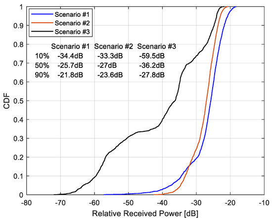
Figure 16. CDF of the relative received power.

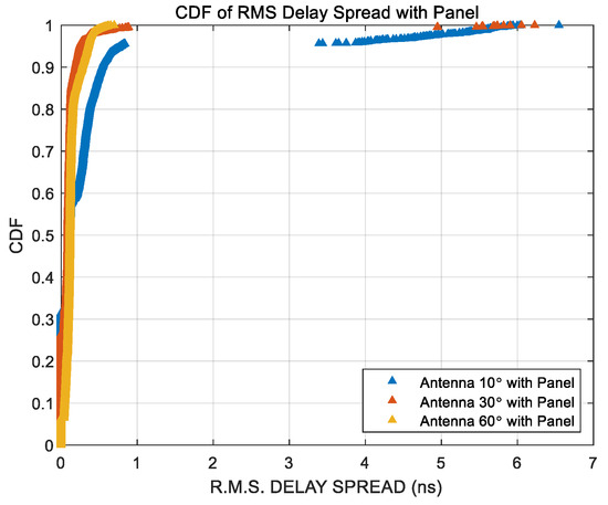
Figure 17. CDF of the R.M.S. delay results for Scenarios #1 to #3.

It is observed that the CDF exhibits relatively larger R.M.S. delay spread values for antenna beamwidths of 10° and 30° compared to 60°. To investigate the underlying cause of this tendency, the R.M.S. delay spread CDFs for each individual scenario are examined in Figure 18, Figure 19 and Figure 20. Among them, Scenario #3 clearly demonstrates a wider distribution of the delay spread, indicating more significant multipath effects. The statistical summary of the R.M.S. delay spread for Scenarios #1 through #3 is presented in Table 5.

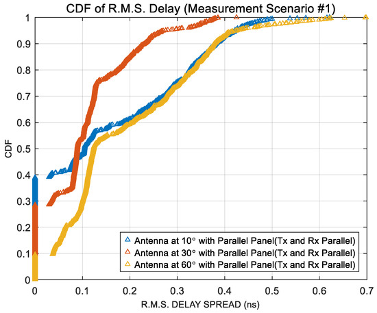
Figure 18. CDF of the R.M.S. delay spread in Scenario #1.

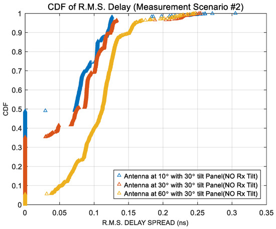
Figure 19. CDF of the R.M.S. delay spread in Scenario #2.

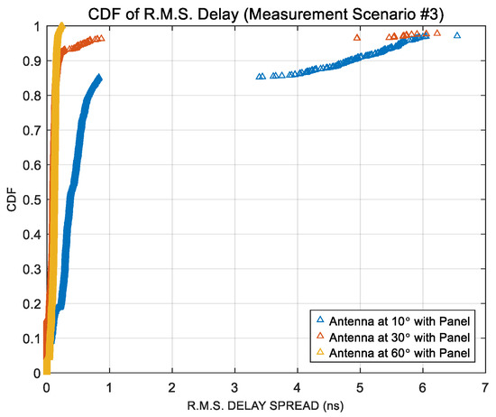
Figure 20. CDF of the R.M.S. delay spread in Scenario #3.

Table 5. Cumulative distribution function values at 10%, 50%, and 90% according to the antenna beamwidth for each measurement scenario.

Scenario	Antenna Beamwidth	10%	50%	90%
#1	10°	0 ns	0.104 ns	0.382 ns
	30°	0 ns	0.089 ns	0.231 ns
	60°	0.038 ns	0.124 ns	0.379 ns
#2	10°	0 ns	0.072 ns	0.120 ns
	30°	0 ns	0.075 ns	0.123 ns
	60°	0.052 ns	0.1112 ns	0.150 ns
#3	10°	0.068 ns	0.369 ns	4.840 ns
	30°	0 ns	0.097 ns	0.178 ns
	60°	0.051 ns	0.118 ns	0.151 ns

In the experimental measurement Scenario #3, as illustrated in Figure 5, the proportion of R.M.S. delay spread values exceeding 1 nanosecond was analyzed based on the antenna beamwidth. The corresponding results are summarized in Table 6. It is evident from the table that narrower beamwidths, particularly 10°, result in a higher percentage of excessive delay spread, indicating increased multipath effects due to refraction or scattering caused by the kiosk panel. Figure 21 presents the cumulative distribution function (CDF) of the R.M.S. delay spread under the condition where the receiver antenna is tilted by 30°, but the kiosk panel is removed. When compared to the CDF of Scenario #3, where the panel is present, it becomes clear that the removal of the panel significantly reduces the distribution range of delay spread. This finding confirms that the presence of the kiosk panel plays a critical role in extending delay times due to signal refraction and internal reflections.

Table 6. Percentage of delay spread greater than 1 nanosecond in measurement Scenario #3.

Antenna Beamwidth	10°	30°	60°
R.M.S Delay Spread > 1 ns (%)	13.2%	1.5%	0%

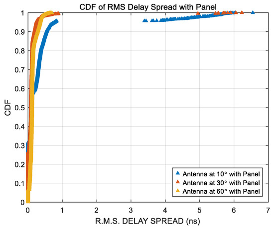
Figure 21. CDF of the R.M.S. delay results in measurement Scenario #3 except for the panel.

Figure 22 shows the CDF of relative received power with and without the kiosk panel for each antenna beamwidth. The relative received power was calculated as the ratio between the measured power and the reference power, which corresponds to the received power at a distance of 10 cm for each beamwidth. The results indicate that received power increases as the antenna beamwidth widens. When averaged across all beamwidths, the total received power was −32.17 dB with the panel and −23.97 dB without it, indicating an average attenuation of approximately 8.2 dB due to the panel. Detailed values of received power for each beamwidth and panel condition are presented in Table 7.

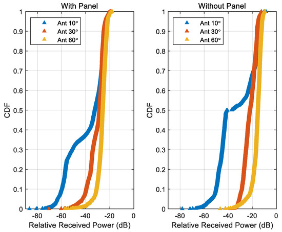
Figure 22. CDF of the relative received power with and without the panel.

Table 7. Relative received power according to antenna beam width and kiosk panel.

Antenna Beamwidth	10°	30°	60°
With the Kiosk Panel	−38.89 dB	−30.99 dB	−26.63 dB
Without the Kiosk Panel	−33.23 dB	−22.24 dB	−16.44 dB

Based on the results shown in Figure 19, Figure 20 and Figure 21, it is confirmed that the variation in the R.M.S. delay spread is more significantly influenced by the presence or absence of the kiosk panel than by the tilt angle of the receiving antenna when using narrow beamwidths of 10° and 30°. In particular, for Scenario #3, which includes a forward-tilted receiver and kiosk panel, the use of narrow beamwidth antennas tends to increase the occurrence of delayed signal components. This is attributed to the fact that signals transmitted from the antenna are more likely to be refracted or reflected by the inclined panel surface before reaching the receiver. Furthermore, narrow beamwidth antennas typically offer higher gain and exhibit lower loss when penetrating the panel material, resulting in a greater likelihood of detecting multipath components that are attenuated by up to 20 dB relative to the strongest impulse in the power delay profile (PDP). This increased probability of capturing delayed signal energy contributes to the broader distribution of R.M.S. delay spread observed under these conditions.

Figure 23 illustrates the impulse response level as a function of delay time, categorized by antenna beamwidth and measurement scenario. The first graph in Figure 23 corresponds to Scenario #2 using a 10° antenna beamwidth. In this plot, the star symbol denotes the peak value of the channel impulse response (CIR), while the red dotted line represents the threshold level, defined as 20 dB below the peak. As per the methodology adopted in this study, only signal components below this threshold are regarded as contributing to delay spread. Accordingly, no delayed signals are observed beyond 5 ns on the time axis in this scenario. The second graph shows the CIR under Scenario #3 with the same 10° beamwidth. Similar to Scenario #2, delayed signal components are not present beyond the 5 ns mark, indicating limited multipath spread under these specific conditions. In contrast, the third graph depicts the results for Scenario #3 using a 60° antenna beamwidth. In this case, additional delayed signals—attenuated below the 20 dB threshold—are observed within the 20 to 25 ns range. The presence of these late-arriving components implies a broader temporal dispersion and, consequently, a larger R.M.S. delay spread. This outcome highlights that, particularly in Scenario #3, both narrow (10°) and wide (60°) beamwidth configurations can yield extended delay profiles due to differing interactions with the kiosk panel and propagation environment.

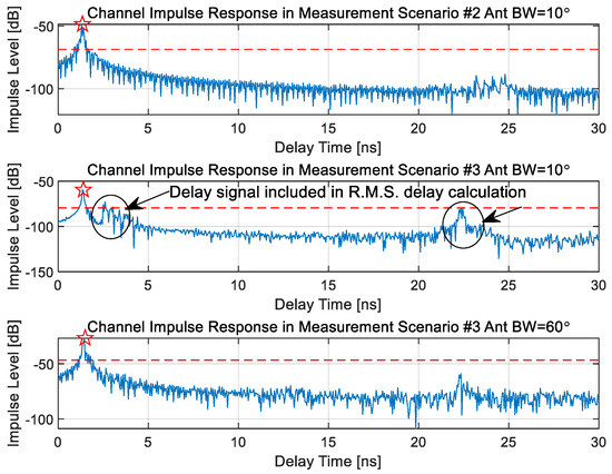
Figure 23. Channel impulse response according to the measurement scenario and antenna beamwidth.

In this study, an R.M.S. delay spread model is derived based on the measurement results obtained from the kiosk data downloading scenario using antennas with varying beamwidths. Figure 24 presents the relationship between the R.M.S. delay spread and relative received power for each beamwidth configuration: 10°, 30°, and 60°. The black dotted line in the figure represents the fitting curve that encompasses all measured data, regardless of beamwidth. The results indicate that when narrow beamwidth antennas (e.g., 10°) are used, the probability of observing larger R.M.S. delay spread values tends to increase, particularly in scenarios where multipath components are more pronounced. This suggests a strong correlation between antenna directivity and delay spread behavior, mediated by the effects of signal focusing and interaction with surrounding materials. In accordance with ITU-R Recommendation P.1238-11, the R.M.S. delay spread can be modeled as a function of path loss, expressed as Equation (1), where A and B are empirical fitting coefficients, and L denotes the path loss. This model enables the prediction of delay characteristics under different propagation conditions and antenna configurations within indoor terahertz systems.

$$Delay Spread=e^{(A\times L+B)}$$

(1)

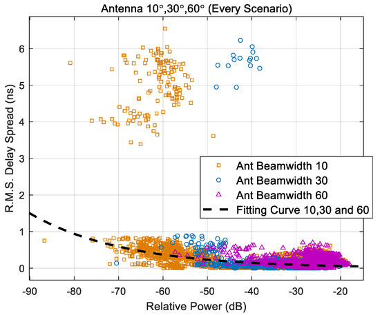
Figure 24. R.M.S. delay spread with relative received power.

The path loss value L in Equation (1) can be equivalently represented by a negative-valued received power, allowing the model to be reformulated as Equation (2). To determine the coefficients A and B for this path loss-based delay spread model, a curve fitting procedure was applied to the measurement data presented in this study. The resulting coefficient values for each antenna beamwidth are summarized in Table 8. Curve fitting was carried out using the Curve Fitting Toolbox in MATLAB R2022b. Specifically, a robust least squares regression method with bi-square weighting was employed to minimize the influence of outliers and enhance the reliability of the model. This approach ensures a more accurate representation of the empirical relationship between received power and R.M.S. delay spread across different antenna configurations.

Table 8. The coefficients of the delay spread model with different values of antenna beamwidth.

\	A	B	${\mathit{R}}^2$
Ant Beamwidth 10	0.05306	−4.156	0.9752
Ant Beamwidth 30	0.02873	−3.46	0.9739
Ant Beamwidth 60	0.0269	−2.694	0.7596
Total	0.04671	−3.801	0.9785

3.2. Rack

Figure 25 presents the cumulative distribution function (CDF) of the relative received power for antenna beamwidths of 30° and 60°, categorized according to the types of obstructions placed between the transmitter and receiver. The relative received power is calculated as the ratio between the measured power and the reference power, where the reference power corresponds to the signal strength measured at a distance of 10 cm for each beamwidth configuration. As expected, the relative received power increases with the widening of the antenna beamwidth due to the broader angular coverage. Figure 26 shows the CDF of the R.M.S. delay spread for each obstruction type—namely, a small mesh panel, a LAN cable, and the case with no obstruction (denoted as “Nothing”)—under 30° and 60° antenna beamwidth conditions. The results indicate that the absence of obstructions results in a narrower delay spread distribution, whereas the presence of obstacles such as mesh panels or LAN cables introduces additional multipath components, thereby increasing the delay spread. This observation confirms that environmental clutter significantly impacts temporal dispersion characteristics, especially when wider beamwidth antennas are employed. The specific values corresponding to the 10%, 50%, and 90% CDF percentiles of R.M.S. delay spread under each configuration are summarized in Table 9.

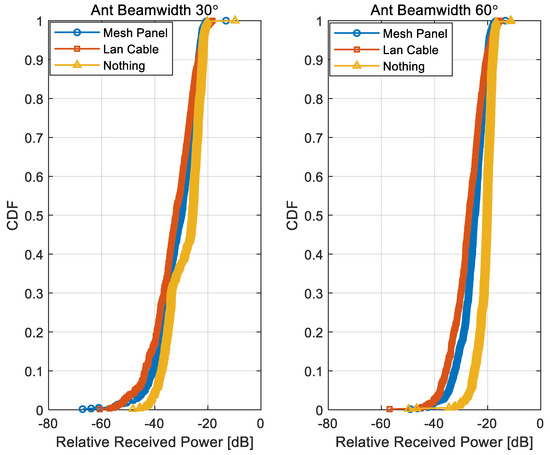
Figure 25. CDF of relative power according to the obstructions.

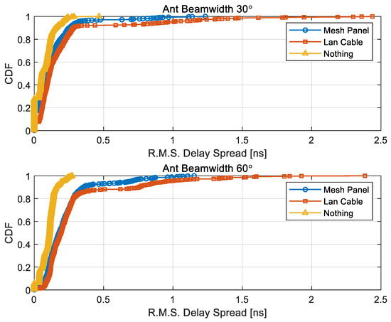
Figure 26. CDF of the R.M.S delay spread according to the obstructions.

Table 9. Cumulative distribution function values at 10%, 50%, and 90% according to the antenna beamwidth for each obstruction and antenna beamwidth.

	Antenna Beamwidth	R.M.S. Delay Spread Coefficient (ns)
		10%	50%	90%
Lan Cable	30°	0.04	0.111	0.281
	60°	0.1	0.194	0.754
Mesh Panel	30°	0	0.098	0.252
	60°	0.08	0.179	0.355
Nothing	30°	0	0.056	0.154
	60°	0.037	0.11	0.157

3.3. Intra-Device

Figure 27 illustrates representative examples of the channel impulse responses for the F–R and F–Sa1 paths in the intra-device measurement scenario. In the figure, the orange line corresponds to the response measured using a 5° beamwidth antenna, while the blue line indicates the result for a 60° beamwidth antenna. The x-axis represents the R.M.S. delay spread in nanoseconds, and the y-axis shows the relative received power level in decibels (dB). Table 10 summarizes the measured values of relative received power and R.M.S. delay spread for all defined propagation paths within the device. The relative received power values were obtained by summing the magnitudes of phase-resolved channel impulse responses, referenced to the calibration level of the transmitter and receiver antennas. Based on these results, R.M.S. delay spread models were developed as a function of the relative received power. To account for structural differences, the delay spread models were categorized according to the physical size of the device enclosure (e.g., large vs. small case). Figure 28 presents the R.M.S. delay spread as a function of relative received power, using the data compiled in Table 11. The resulting trends reveal a clear distinction based on device size; however, no significant correlation is observed with respect to antenna beamwidth. Therefore, for intra-device environments, the R.M.S. delay spread can be more accurately modeled by considering the combination of received power and case size, rather than antenna directivity. One such model follows the general form of Equation (1), where A and B are empirically derived coefficients and L denotes path loss.

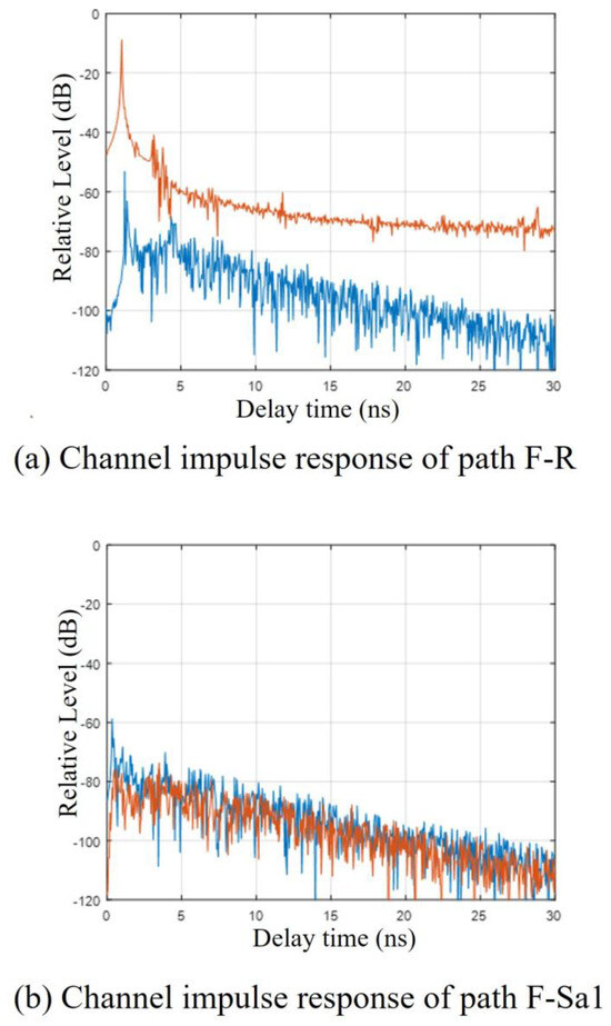
Figure 27. Examples of the channel impulse response. (Orange line: 5 deg beamwidth, Blue line: 60 deg beamwidth).

Table 10. Received level and R.M.S. delay spread in the intra-device scenario.

Radio Path			F_R	F_Sa1	F_Sa2	F_Sa3	F_Sa4	F_Sa5	Sb1_Sa1
Relative received level (dB)	Big	5°	−7.58	−69.78	−57.64	−52.12	−55.47	−56.27	−73.08
		10°	−21.99	−73.84	−56.92	−61.64	−64.17	−57.04	−42.36
		60°	−51.87	−57.52	−56.55	−64.54	−60.46	−68.83	−61.98
	Small	5°	−9.41	−73.87	−57.12	−51.67	−62.17	−58.21	−59.57
		10°	−21.23	−65.07	−56.56	−63.80	−60.81	−54.69	−51.74
		60°	−53.43	−48.21	−57.65	−52.84	−50.57	−62.56	−51.15
Radio Path			Sb1_Sa2	Sb1_Sa3	Sb2_Sa1	Sb2_Sa2	Sb2_Sa3	Sb2_Sa4	Sb2_Sa5
Relative received level (dB)	Big	5°	−59.48	−0.44	−66.5	−57.75	−52.6	−54.65	−0.13
		10°	−39.60	−10.93	−60.07	−59.74	−54.99	−43.2	−11.43
		60°	−52.82	−49.95	−67.99	−58.03	−57.57	−50.14	−39.82
	Small	5°	−52.88	−0.83	−60.83	−61.96	−46.10	−60.28	−1.60
		10°	−44.45	−7.22	−63.54	−60.33	−47.92	−52.72	−7.08
		60°	−43.15	−38.69	−61.01	−54.98	−49.58	−42.50	−38.24
Radio Path			F_R	F_Sa1	F_Sa2	F_Sa3	F_Sa4	F_Sa5	Sb1_Sa1
R.M.S. delay spread (ns)	Big	5°	0.099	5.396	4.326	5.091	3.51	3.401	3.978
		10°	0.586	5.43	4.824	5.517	5.757	4.659	3.363
		60°	2.450	4.023	4.374	5.112	4.924	4.927	4.177
	Small	5°	0.334	2.436	2.729	2.455	2.707	2.750	2.749
		10°	1.069	3.259	2.7	2.768	2.898	2.435	2.226
		60°	1.707	1.904	2.128	2.386	2.119	2.536	1.746
Radio Path			Sb1_Sa2	Sb1_Sa3	Sb2_Sa1	Sb2_Sa2	Sb2_Sa3	Sb2_Sa4	Sb2_Sa5
R.M.S. delay spread (ns)	Big	5°	3.824	0.001	4.854	5.238	5.144	4.186	0.116
		10°	3.127	0.224	4.893	5.625	3.316	2.553	0.218
		60°	2.789	1.855	4.354	4.571	3.166	1.967	0.652
	Small	5°	2.424	0.177	2.523	2.579	1.443	1.502	0.197
		10°	2.128	0.177	2.593	2.984	1.866	1.763	0.211
		60°	1.558	1.019	1.992	1.957	1.564	1.264	0.846
Board distance (mm)			70		90		110		130
Radio Path			Ba_Bb1	Ba_Bb2	Ba_Bb1	Ba_Bb2	Ba_Bb1	Ba_Bb2	Ba_Bb1	Ba_Bb2
Relative received level (dB)	Big	5°	−7.86	−70.25	−12.01	−69.36	−14.85	−71.39	−17.10	−66.00
		10°	−12.32	−63.87	−11.81	−66.59	−12.13	−61.41	−16.00	−61.98
		60°			−45.99	−54.94	−41.54	−65.26	−42.34	−52.49
	Small	5°	−4.34	−77.98	−3.13	−69.49	−5.04	−63.73
		10°	−4.43	−74.03	−6.69	−69.09	−9.6	−63.83
		60°	−31.78	−63.62	−40.40	−56.21	−41.74	−62.28
R.M.S. delay spread (ns)	Big	5°	0.358	3.328	0.416	3.064	0.347	3.074	0.413	3.712
		10°	0.21	3.508	0.266	3.335	0.326	2.589	0.296	2.446
		60°			0.591	2.38	1.252	2.927	1.447	2.396
	Small	5°	0.222	1.395	0.334	1.356	0.442	1.178
		10°	0.076	1.442	0.128	1.394	0.11	1.494
		60°	0.193	1.302	0.253	1.448	0.618	1.269
Board distance (mm)			30		50		70

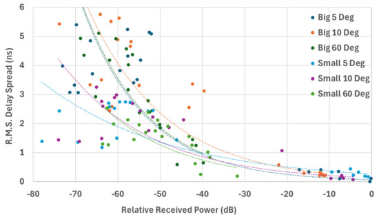
Figure 28. R.M.S. delay spread with relative received power. (The colored lines represent the respective trend lines).

Table 11. The coefficients of delay spread.

	$\alpha$	$\beta$	$R^2$
Big	−0.03	−0.5	0.653
Small	−0.02	−0.5	0.514

The path loss can be changed to relative received power, P with a negative value, then it becomes Equation (2).

$$Delay Spread=e^{(-\alpha \times P+\beta )}$$

(2)

The coefficients of the delay spread model are shown in Figure 27 and Equation (2) is shown in Table 11, and their coefficients of determination, R2, are shown.

The R.M.S. delay spread values were calculated from the measured channel impulse responses, with a threshold level set to 20 dB below the first peak of the power delay profile (PDP). Figure 29 presents the PDPs for various device sizes, showing the temporal distribution of multipath components in the intra-device environment. Figure 30 summarizes the cumulative distribution function (CDF) of the R.M.S. delay spread values. Specifically, the 10th, 50th, and 90th percentile values are 0.273 ns, 0.927 ns, and 2.374 ns, respectively. These results reflect significant temporal dispersion, which can degrade system performance through inter-symbol interference (ISI). To estimate the upper bound on data transmission rate while avoiding ISI, the relationship R < 1/(2τd)R < 1/(2τ_d)R < 1/(2τd) was applied, where τdτ_dτd is the R.M.S. delay spread. Based on the average delay spread of 1.3039 ns, the maximum achievable transmission rate is approximately 0.38 Gbps, assuming no equalization or diversity techniques are used. For the worst-case delay spread of 4.409 ns, the rate drops to 0.113 Gbps. Even under the best-case scenario with a delay spread of 0.01 ns, the theoretical upper bound reaches 50 Gbps. Nonetheless, due to the inherent multipath effects observed in intra-device propagation, achieving multi-gigabit rates remains challenging without advanced mitigation techniques. The statistical parameters of the R.M.S. delay spread for intra-device environments are detailed in Table 12. Additionally, Figure 31 displays the fitted R.M.S. delay spread model for various device sizes when using antennas with a beamwidth of 60°, further emphasizing the impact of physical dimensions on channel temporal dispersion. Figure 32 presents the relationship between R.M.S. delay spread and relative received power for intra-device environments. The red line represents the curve fitted across all measured data points, encompassing various device sizes, with the antenna beamwidth fixed at 60°. The trend indicates a clear dependence of delay spread on received power, which reflects the impacts of multipath components and the device structure. In accordance with ITU-R Recommendation P.1238-11, the R.M.S. delay spread can be modeled as a function of path loss, as expressed in Equation (1). Since path loss can be represented as a negative value of received power, the model can be equivalently reformulated into Equation (2) using the relative received power as the input variable. To determine the model coefficients A and B, curve fitting was conducted based on the measurement data obtained in this study. The fitting process was applied specifically to intra-device scenarios involving all case sizes and a 60° antenna beamwidth configuration. The resulting delay spread model parameters are presented in Equation (3), which characterizes the statistical behavior of delay spread in response to signal attenuation within the intra-device environment.

$$Delay Spread=e^{(-0.017\times P-0.272)}$$

(3)

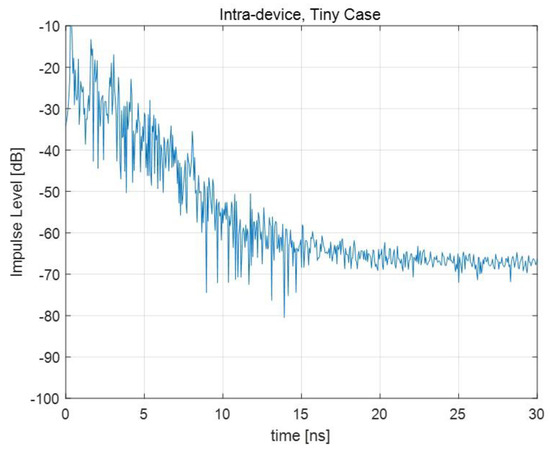
Figure 29. Measured PDP for the intra-device environment (tiny).

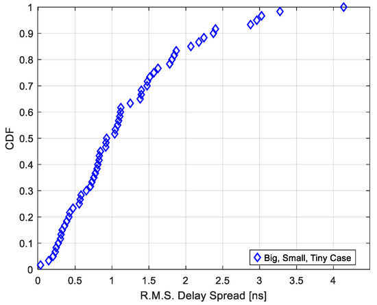
Figure 30. CDF for the intra-device environment.

Table 12. Statistics of the R.M.S. delay spread for intra-device environments.

Statistics	Max	Min	Average	Median	STD
R.M.S. delay spread (ns)	4.139	0.032	1.197	0.982	0.875

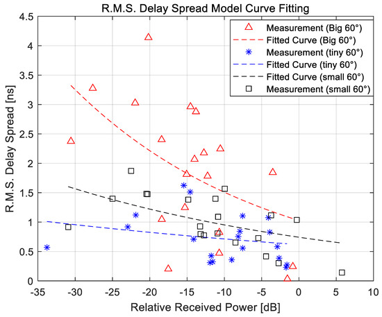
Figure 31. R.M.S. delay spread model for the intra-device environment according to the device size (antenna beamwidth of 60°).

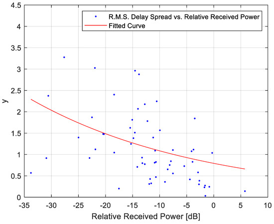
Figure 32. R.M.S. delay spread model for all device cases and beamwidths.

3.4. Experimental Laboratory Environment

Figure 33 presents the measurement results of selected receiver positions in the experimental laboratory environment, visualized as a three-dimensional plot and its corresponding contour map. The graphs depict relative received power versus delay time across different spatial links. At the link between transmitter location 1 and receiver location 1, the first peak appears over a wide azimuth range due to the broad beamwidth of the measurement antenna. For the link between transmitter location 1 and receiver location 7, a second peak emerges following the first, and a third peak is observed when the receiver is oriented at ±180°, which is presumed to result from reflection off the entrance door wall. In contrast, the links from transmitter location 2 exhibit a more complex multipath behavior than those from transmitter location 1. Specifically, for the link between transmitter location 2 and receiver location 1, the primary peak is observed off-center, likely due to the off-axis placement of the transmitter. Additionally, for links between transmitter location 2 and receiver locations 4 and 7, a greater number of reflected components are observed compared to the corresponding links from transmitter location 1. This increase is attributed to additional reflections not only from the end wall but also from the side walls of the measurement space. Based on the measurement data across all receiver positions, the strongest received power levels were extracted and used to estimate path loss as a function of distance. The results are shown in Figure 34, where the blue dotted line represents the curve fitted to the strongest measured values, and the red line denotes the theoretical free-space path loss model. The extracted path loss exponent is approximately 1.95, which is closely aligned with the ideal free-space attenuation coefficient of 2.0, indicating a predominantly line-of-sight propagation condition within the measurement environment.

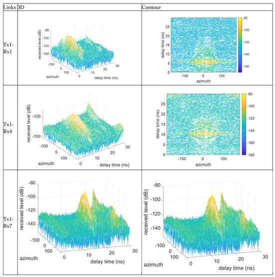
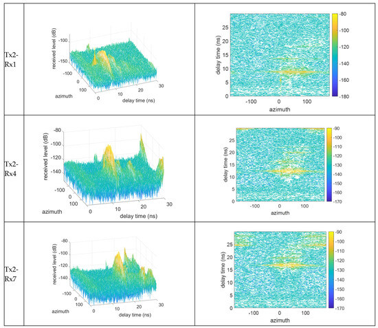
Figure 33. Results at some links and 3D and contour plots.

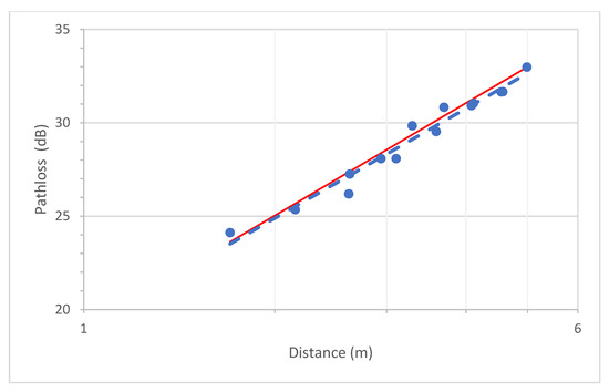
Figure 34. Path loss of selected the strongest levels. (The dots are actual measurements, the dotted lines are trend lines).

Figure 35 presents the relationship between the R.M.S. delay spread and path loss, as derived from the experimental measurement results in the laboratory environment. The delay spread values were calculated from multipath components extracted from the power delay profiles (PDPs), applying a threshold level set at 20 dB below the peak signal amplitude. The observed trend demonstrates that the R.M.S. delay spread increases with greater path loss, indicating more significant temporal dispersion under weaker received signal conditions. This relationship can be effectively characterized by an exponential function, capturing the nonlinear growth of delay spread with increasing signal attenuation.

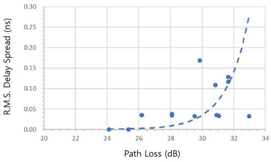
Figure 35. Picture of measurements at Tx1 and Tx2. (The dots are actual measurements, the dotted lines are trend lines).

4. Conclusions

In this study, power delay profiles (PDPs) were obtained using a vector network analyzer (VNA) and frequency extenders across four representative scenarios: the kiosk data downloading environment, the inter-rack communication environment in a data center, the intra-device communication environment, and the controlled experimental laboratory setting. Based on the extracted PDPs, R.M.S. delay spread values were analyzed to quantify multipath propagation effects in the 275–295 GHz terahertz band.

For each scenario, cumulative distribution functions (CDFs) and statistical coefficients of R.M.S. delay spread were derived. In the kiosk environment, a delay spread model was established as a function of the antenna beamwidth, highlighting the impact of directivity on temporal dispersion. In the inter-rack scenario, the 10%, 50%, and 90% delay spread percentiles were quantified for varying antenna beamwidths and the presence of obstructions such as LAN cables and mesh panels. For intra-device communication, the delay spread model was developed based on the device enclosure size and antenna beamwidth, emphasizing the structural influence on delay characteristics. In the laboratory environment, the relationship between R.M.S. delay spread and path loss was investigated, and the trend was successfully modeled using an exponential fitting function.

The findings presented in this paper provide key insights into the propagation behavior and system design considerations for future short-range wireless communication systems operating in the 285 GHz band. These results contribute to the foundation for deploying terahertz systems in practical environments. Future work will extend this analysis to the 400 GHz band using similar experimental scenarios to further enhance the understanding of propagation mechanisms in the low-THz spectrum.

References

- Abbasi, A.; Kishk, M.A.; Alouini, M.-S. A survey on terahertz communications: Applications, research challenges, and standardization activities. IEEE Open J. Commun. Soc. 2021, 2, 1266–1292. [Google Scholar]
- Rappaport, T.S.; Xing, Y.; MacCartney, G.R., Jr.; Molisch, A.F.; Mellios, E.; Zhang, J. Wireless communications and applications above 100 GHz: Opportunities and challenges. IEEE Access. 2019, 7, 78729–78757. [Google Scholar] [CrossRef]
- Han, C.; Wu, Y.; Chen, Z.; Wang, X. Terahertz channel modeling for wireless communications—A survey. IEEE Commun. Surveys Tuts. 2021, 23, 2174–2214. [Google Scholar]
- Jornet, J.M.; Akyildiz, I.F. Channel modeling and capacity analysis for electromagnetic wireless nanosensor networks in the terahertz band. IEEE Trans. Wireless Commun. 2011, 10, 3211–3221. [Google Scholar] [CrossRef]
- Sarieddeen, H.; Alouini, M.-S.; Al-Naffouri, T.Y. An overview of signal processing techniques for terahertz communications. Proc. IEEE 2021, 109, 1628–1665. [Google Scholar] [CrossRef]
- Samimi, M.K.; Rappaport, T.S. 3-D millimeter-wave statistical channel model for 5G wireless system design. IEEE Trans. Microw. Theory Techn. 2016, 64, 2207–2225. [Google Scholar] [CrossRef]
- ITU. ITU-R Recommendation P.1238-11, Propagation Data and Prediction Methods for the Planning of Indoor Radiocommunication Systems and Radio Local Area Networks in the Frequency Range 300 MHz to 450 GHz; International Telecommunication Union: Geneva, Switzerland, 2021. [Google Scholar]
- Kürner, T.; Priebe, S. Towards THz communications—Status in research, standardization and regulation. J. Infrared Millim. Terahertz Waves 2014, 35, 53–62. [Google Scholar] [CrossRef]
- Tekbıyık, K.; Uysal, M. Indoor terahertz wireless communications: Measurement, modeling and future directions. IEEE Access 2022, 10, 114567–114582. [Google Scholar]
- Pi, Z.; Khan, F. An introduction to millimeter-wave mobile broadband systems. IEEE Commun. Mag. 2011, 49, 101–107. [Google Scholar] [CrossRef]
Disclaimer/Publisher’s Note: The statements, opinions and data contained in all publications are solely those of the individual author(s) and contributor(s) and not of MDPI and/or the editor(s). MDPI and/or the editor(s) disclaim responsibility for any injury to people or property resulting from any ideas, methods, instructions or products referred to in the content. |
© 2025 by the authors. Licensee MDPI, Basel, Switzerland. This article is an open access article distributed under the terms and conditions of the Creative Commons Attribution (CC BY) license (https://creativecommons.org/licenses/by/4.0/).