Article

An Ensemble Learning Approach for Facial Emotion Recognition Based on Deep Learning Techniques

by
Manal Almubarak
and
Fawaz A. Alsulaiman
*
Department of Computer Science, College of Computer and Information Sciences, King Saud University, Riyadh 11543, Saudi Arabia
*
Author to whom correspondence should be addressed.
Electronics 2025, 14(17), 3415; https://doi.org/10.3390/electronics14173415
Submission received: 29 June 2025 / Revised: 17 August 2025 / Accepted: 24 August 2025 / Published: 27 August 2025

Abstract

Facial emotion recognition (FER) is an evolving sub-field of computer vision and affective computing. It entails the development of algorithms and models to detect, analyze, and interpret facial expressions, thereby determining individuals’ emotional states. This paper explores the effectiveness of transfer learning using the EfficientNet-B0 convolutional neural network for FER, alongside the utilization of stacking techniques. The pretrained EfficientNet-B0 model is employed to train on a dataset comprising a diverse range of natural human face images for emotion recognition. This dataset consists of grayscale images categorized into eight distinct emotion classes. Our approach involves fine-tuning the pretrained EfficientNet-B0 model, adapting its weights and layers to capture subtle facial expressions. Moreover, this study utilizes ensemble learning by integrating transfer learning from pretrained models, a strategic tuning approach, binary classifiers, and a meta-classifier. Our approach achieves superior performance in accurately identifying and classifying emotions within facial images. Experimental results for the meta-classifier demonstrate 100% accuracy on the test set. For further assessment, we also train our meta-classifier on a Cohn–Kanade (CK+) dataset, achieving 92% accuracy on the test set. These findings highlight the effectiveness and potential of employing transfer learning and stacking techniques with EfficientNet-B0 for FER tasks.

1. Introduction

Facial emotion recognition (FER) technology represents a considerable breakthrough in recognizing human emotions and intentions. In the evolving field of FER, deep learning (DL) is a crucial development, using the computational power of neural networks for the detection and interpretation of a wide range of facial emotional expressions. In human communication, information is transferred from one person to another using two levels of communication: verbal communication and non-verbal communication. Some studies have suggested that 60–80% of our communication is non-verbal [1]. Facial emotions are categorized as a form of non-verbal communication that augments verbal communication and plays a vital role in our communication and connection with others.
Nowadays, many businesses rely on feedback questionnaires, which many customers either ignore or fill in without paying sufficient attention to the questions. Some businesses offer incentives for writing feedback, but this method is generally ineffective because there is no mechanism to ensure that customer-provided feedback is sincere. In this context, FER technology has value across several sub-domains of human–computer interaction, including psychological analysis, healthcare, working environments, tendency towards crime, etc. By leveraging advancements in computer vision and machine learning (ML) techniques, we contribute to the evolution of FER systems by enhancing the detection and interpretation of a wide range of facial expressions across diverse populations in real time, with low latency and high efficiency. Our motivation is to provide an accurate system that can automatically capture the underlying emotional cues expressed when we communicate, interact, and empathize with each other. FER involves technology that analyzes human facial features and detects and interprets emotions based on facial expressions. Several existing studies [2,3,4,5,6,7,8,9,10,11,12,13,14,15] have attempted to address a variety of issues related to FER, utilizing classical ML techniques such as support vector machine (SVM), random forest, and k-nearest neighbors (k-NN) or DL techniques such as convolutional neural networks (CNNs) and recurrent neural networks (RNNs).
The EfficientNet-B0 model is used in this study due to its effectiveness in image classification tasks, particularly when trained on diverse datasets [16]. Attaining high accuracy across diverse datasets is crucial in ensuring the model’s robustness and generalizability, particularly in real-world FER applications such as online learning, healthcare, and human–computer interaction systems. The goal of this paper is to determine and classify individuals’ emotions by leveraging the DL EfficientNet-B0 model and to explore its efficacy. The initialization, training, and evaluation of the model were conducted via Google Colaboratory notebooks, commonly referred to as “Colab”, which is a cloud-based service provided by Google [17] that permits access to computing units for code execution, access to GPUs, and the utilization of high-memory machines. The dataset used in this paper consists of image data. However, it is important to note that the EfficientNet-B0 model requires fixed-sized input images, typically set at 224 × 224 pixels, which can consume a significant amount of memory during the model training phase.
One important factor that significantly impacts the performance of EfficientNet-B0 is the quality of the collected dataset and the quantity of the training data. Although EfficientNet-B0 is renowned for its efficiency in terms of parameters and computational resources, it still possesses a certain level of complexity that necessitates thorough training, fine-tuning, and significant computational resources. DL models, especially when dealing with small datasets, are prone to overfitting. Overfitting arises when the model converges to a solution that fits the training data excessively, i.e., by capturing misleading details such as noise and outliers. This reduces its generalization capability, which is crucial when the model is applied to unseen data [18]. Techniques such as data augmentation, regularization, and dropout can help to mitigate overfitting, but they may not completely eliminate it. Furthermore, from an ethical standpoint, FER technology raises concerns related to privacy, consent, bias, and potential misuse. Careful consideration of these ethical aspects is crucial component of our analysis throughout this paper, i.e., from data collection and model development to deployment and usage.
This paper is structured as follows: Section 2 presents the general background information about CNNs and the selected CNN algorithm (EfficientNet-B0); Section 3 reviews the existing literature related to different types of ML and deep CNN approaches in the field of FER; Section 4 explains the methodology employed to classify a person’s dominant emotion based on their facial expression; Section 5 details the experiment, including a description of the dataset, the tools used to conduct the experiment, and the metrics used to measure the performance. Finally, Section 6 presents the conclusions and suggests directions for future research.

2. Background

This section first provides background information on the concept of facial emotion recognition, followed by an overview of machine learning techniques, starting with traditional approaches such as decision trees (DTs) and support vector machine (SVM) and then proceeding to more advanced deep learning methods, including CNNs and the EfficientNet architecture. Finally, ensemble learning approaches such as bagging, boosting, and stacking are examined.

2.1. FER

Facial expression recognition (FER) is a fascinating and rapidly evolving area within the broader field of computer vision, and it plays an important role in enabling the automated capture of human emotional information, which is a key aspect of affective computing. It involves the development of algorithms and models to detect, analyze, and interpret facial expressions to infer a person’s emotional states. The ability to recognize emotions from facial cues is crucial for various applications, including human–computer interaction, virtual reality, healthcare, and social robotics. Paul Ekman and Wallace V. [19] laid the groundwork for research on facial emotion recognition in the 1970s by identifying a set of universally recognized facial expressions corresponding to basic emotions, namely happiness, sadness, anger, fear, surprise, and disgust. With the advent of powerful computing and advancements in computer vision, researchers began to leverage ML and DL techniques to automate the process of emotion recognition from facial features.

2.2. ML and DL Techniques

With the integration of ML and DL techniques, FER has achieved significant advancements. The intersection of computer vision and affective computing aims to automate the identification and interpretation of emotional states through facial expressions, offering widespread applications in human–computer interaction.

2.2.1. Traditional Approaches

Early approaches in FER relied on handcrafted features and rule-based systems [20]. As the field evolved, researchers sought more sophisticated solutions to enhance the accuracy and generalization. Below are some examples of traditional approaches.
Facial Action Coding System (FACS): Developed by Ekman and Friesen in 1978, the FACS investigates facial expressions through the observation of specific facial muscles’ activity, which is described using action units (AUs). Each AU corresponds to the movement of one or more facial muscles, and combinations of AUs represent distinct facial expressions. Ekman and Friesen found that a single facial expression can be represented by up to 46 action units [21]. There are several numerical codes for each AU to specify the muscle or muscle groups being moved in the expression [22]. Moreover, many studies have proposed methods of detecting AU occurrence and AU intensity [23,24,25,26,27,28].
Gabor Wavelets: Named after the Hungarian-born electrical engineer Dennis Gabor, who proposed them in the 1946 [29], Gabor wavelets are practical in face recognition and have been applied to capture facial texture information by convolving images with Gabor filters at different scales and orientations [30].
Local Binary Patterns (LBPs): An LBP is a texture descriptor that measures local patterns in an image [31]. It has been used to encode facial texture by comparing the intensity of pixels in a local neighborhood [32]. Facial expressions often involve specific patterns of texture changes, such as wrinkles around the eyes or mouth. LBP features are typically represented using histograms to statistically describe image characteristics [31].

2.2.2. ML Paradigms

ML techniques marked a paradigm shift in FER. Classifiers were employed to discern patterns within facial feature representations. Feature extraction played a crucial role, with methods like LBPs aiding in the identification of discriminative facial features. In ML, the process of learning is performed by classifiers. Below are some examples of traditional approaches [33].
Support Vector Machine (SVM): SVM is a supervised machine learning algorithm commonly employed for classification and regression tasks. Rather than performing classification in the original feature space, SVM transforms the data into a higher-dimensional space, where a linear hyperplane can be identified to separate the classes, while maximizing the margin between the support vectors, as shown in Figure 1. When mapped back to the original feature space, this hyperplane becomes non-linear and serves as a decision boundary that separates the classes [34]. SVM was originally designed for binary classification tasks to separate data points into two classes, but it can be extended to handle multiple classes through a variety of approaches. There are two main techniques to adapting SVM for multiclass classification.
  • One-to-one approach, where a binary SVM classifier is trained for each pair of classes. If there are m classes, this results in the following [35]:
    m × ( m 1 ) 2 S V M s
  • One-to-rest approach, where a binary SVM classifier is trained for each class. If there are m classes, one class is selected and designated as the positive class, while all other classes are treated as the negative class. By iteratively considering each of the m classes as the positive class, the original multiclass classification problem is transformed into m separate binary classification problems. Each classifier then determines whether a given instance belongs to its respective positive class or not [35].
Decision Tree (DT): A DT is a supervised machine learning algorithm commonly utilized for classification and regression tasks. It is considered an interpretable model, as it reveals the decision-making logic rather than operating as a black-box classifier. Its structure resembles a tree that expands into decision branches and leaf nodes. Each internal node evaluates a condition that directs the flow toward subsequent branches or leaf nodes. Each leaf node represents a final decision, typically denoted as a class label. The construction of a DT involves recursively partitioning the training data into subsets based on the most informative features, aiming to maximize the homogeneity of the resulting subsets [36].
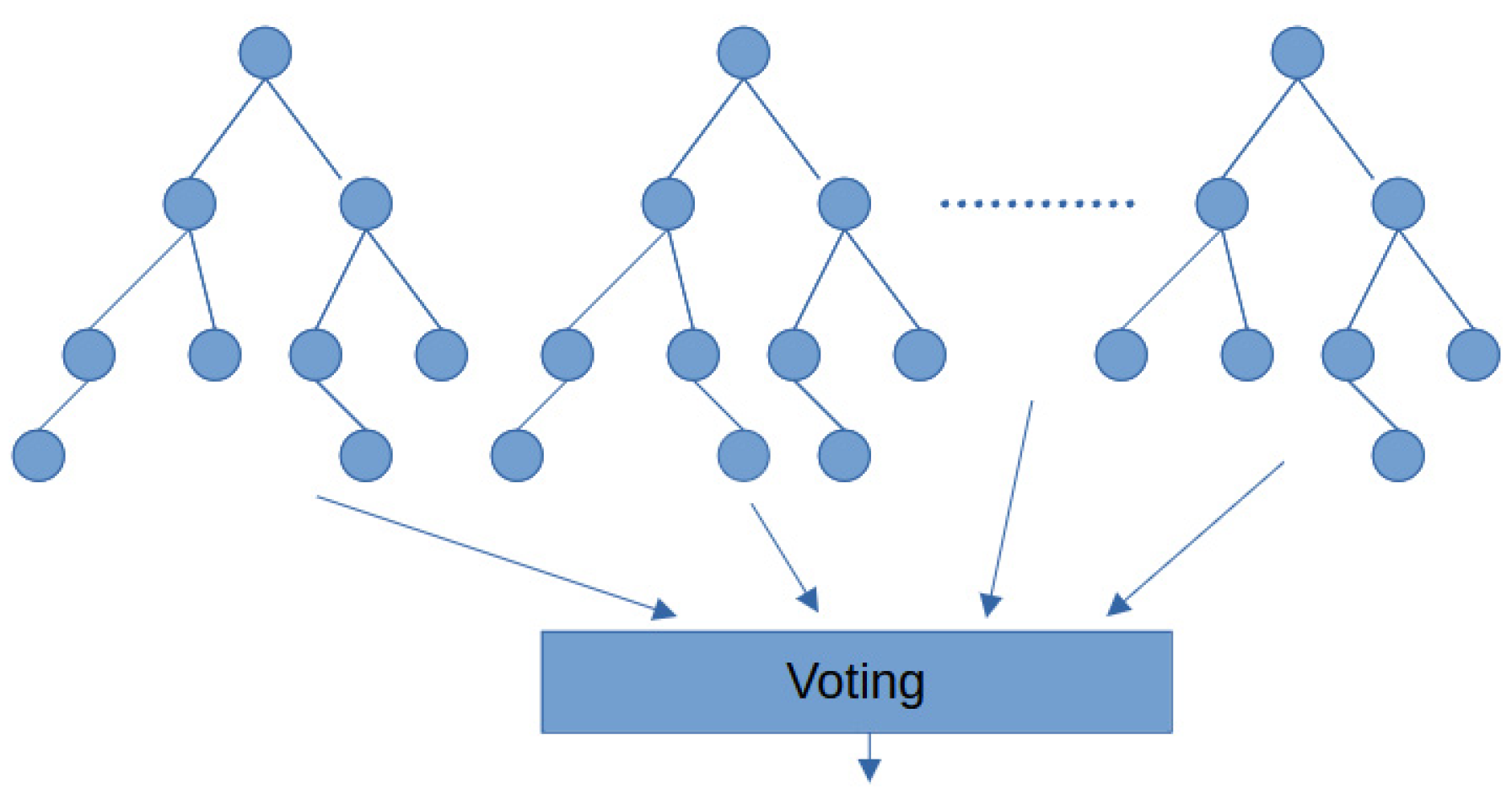
Random Forest (RF): RF is a powerful learning method in ML that is used to address both classification and regression problems. It contains the output of a collection of DTs to predict a single result that is more accurate, reducing the risk of overfitting, as shown in Figure 2. RF provides flexibility, but it is a time-consuming process since it handles large datasets, which require more resources and higher computational complexity [37].
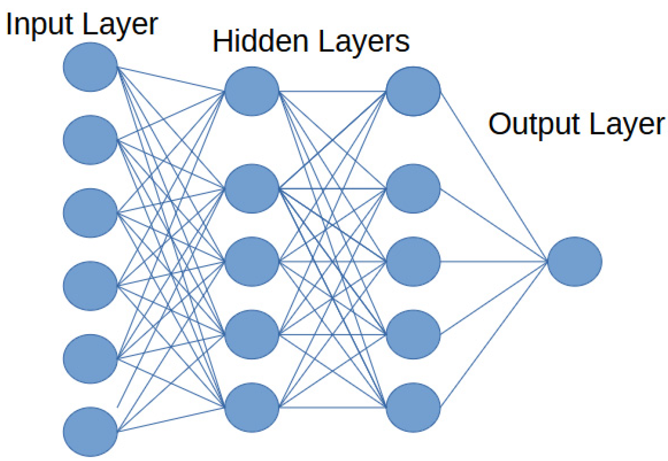
Multilayer Perceptron (MLP): MLP is a neural network architecture in machine learning, composed of three main types of layers: an input layer, which receives the feature vectors; one or more hidden layers, consisting of neurons with connection weights and activation functions; and an output layer, which produces the final prediction. The hidden and output layers of the nodes utilize forward propagation and non-linear activation functions to classify data that are not linearly separated. Figure 3 shows an example of an MLP architecture. The process of training involves the backward propagation of errors to adjust the weights using optimization techniques [33].

2.2.3. Rise of DL

The emergence of DL, and particularly CNNs, revolutionized FER and led to remarkable breakthroughs in its accuracy. CNN and RNN algorithms have been utilized for the purpose of feature extraction, classification, and recognition tasks. CNN is one of the most widely used network models among the various deep learning models. A CNN consists of three types of heterogeneous layers [38].
  • Convolution layers: These perform convolution operations on the input data using a collection of filters to produce feature maps that reflect and represent the spatial characteristics of the facial image.
  • Max pooling layers: In these layers, a form of dimensionality reduction is performed by reducing the spatial resolution of the feature maps. This operation helps to focus on the most relevant features while discarding less significant details.
  • Fully connected layers: These layers are typically found at the end of a CNN and are often followed by activation functions. Fully connected layers utilize the high-level features extracted by the preceding layers to perform predictions or classifications. Figure 4 shows a CNN architecture that consists of convolution layers, pooling layers, and fully connected layer.

2.3. EfficientNet

EfficientNet is a CNN architecture designed for image classification tasks, representing a significant milestone in the growth of CNN architectures to improve their performance. The EfficientNet model was developed by Mingxing Tan and Quoc V. Le at Google Research [16]. They proposed a method known as compound scaling to quantify the relationship between all three network dimensions, namely the depth, width, and resolution. They used a neural architecture search to propose a method that scales these three dimensions simultaneously, with a constant ratio on the new baseline network, in order to achieve better accuracy and efficiency. The model is scaled using the following three parameters [16].
Depth (d)—increasing the number of layers. This is a method used commonly by many convolutional networks to extract more complex features. It is used with a number of techniques to reduce and moderate the gradient problems that pertain to training, such as skip connection [39] and batch normalization [40].
Width (w)—increasing the number of channels to extract more fine-grained features. This method is used widely with small-sized models.
Resolution (r)—increasing the number of pixels for the input images to extract more fine-grained patterns at a high resolution. This started from 224 × 224 r in early CNNs, followed by 229 × 229 or 331 × 331 r to attain better accuracy and then GPipe with a 480 × 480 resolution; finally, some other CNNs work with a 600 × 600 resolution.
Tan and Quoc V. Le [16] noted that larger networks, with a larger w, d, or r (employing single-dimension scaling), achieve better accuracy, but this accuracy will deteriorate after reaching 80% for larger models. During CNN scaling, they recommend balancing all network dimensions to achieve higher accuracy and efficiency. They applied a compound coefficient, ϕ, to balance the scaling of the three dimensions as follows:
D e p t h : d = α ϕ W i d t h : w = β ϕ R e s o l u t i o n : r = γ ϕ s . t .   α .   β 2 .   γ 2 2 α 1 ,   β 1 ,   γ 1
The scaling coefficients α, β, and γ are constants that determine the extent to which the d, w, and r should be scaled, respectively. The coefficient ϕ is a user-defined scaling factor that regulates the resources allocated for model scaling. Moreover, they proposed a constraint on the scaling coefficients such that α, β 2 . γ 2 is a constant to balance between the three dimensions and maximize the performance of the model. Consequently, with each increase in the scaling coefficient, ϕ, the total FLOPS scales proportionally to 2 ϕ . The demonstration of the scaling method in [16], where the EfficientNet model was proposed, was based on the existing MobileNet [41,42] and ResNet [43] models. Recent neural networks have achieved high accuracy by tuning architectural parameters such as the network width, depth, convolution types, and sizes. However, a significant gap remains, particularly when applied to larger datasets: these models often require extensive and computationally expensive hyperparameter tuning. In this context, the EfficientNet architecture was designed with compound scaling to bridge this gap, achieving better accuracy with larger datasets. The EfficientNet architecture consists of a baseline network, referred to as EfficientNet-B0, and variants such as B1, B2, …, B7, which denote different scaling factors. The baseline architecture includes mobile inverted bottlenecks like MobileNetV2, but with additional enhancements. The baseline network EfficientNet-B0 was developed using the same search space as in [44], with the use of the objective function ACC(m) × [FLOPS(m)/T]w, where ACC(m) refers to the accuracy of model m, FLOPS(m) refers to the FLOPS of model m, T refers to the target FLOPS, and w = 0.07, which is a hyperparameter employed to balance accuracy and FLOPS. After establishing the baseline network, scaling is performed by applying the following two steps.
Step 1: The compound coefficient is fixed at ϕ = 1; then, the optimal scaling factors for EfficientNet-B0 are empirically determined as α = 1.2, β = 1.1, and γ = 1.15 under the constraint of α. β 2 . γ 2   2 .
Step 2: To obtain EfficientNet-B1 to -B7, the constants α, β, and γ are fixed and the baseline network is scaled up using various values of ϕ via Equation (2).
The experiment of Tan and Quoc V. [16] started with the application of their scaling method to the MobileNet and ResNet models; they found that the accuracy improved in all these models. They then applied the EfficientNet models to the ImageNet dataset. It is important to note that the dropout ratio increased linearly from 0.2 for EfficientNet-B0 to 0.5 for EfficientNet-B7, as larger models require additional regularization. They determined that all EfficientNet models achieved better accuracy, with fewer parameters and FLOPS, than other CNNs, which makes EfficientNet the favorable and optimal choice in terms of accuracy, performance, and efficiency. Moreover, after running many experiments on real CPUs to validate the latency, the authors determined that EfficientNets are fast on real hardware. EfficientNet has demonstrated excellent performance compared to other network architectures, achieving high accuracy with fewer parameters and a lower computational cost. It should be noted that the compound scaling method achieved up to 2.5% higher accuracy than the best of the other single-dimension scaling methods. EfficientNets performed well on the ImageNet dataset, and they were tested on eight widely used datasets, achieving high accuracy on five out of these eight datasets, with a smaller number of parameters—by up to 21 times compared to the previous CNNs. The EfficientNet architecture has found application in diverse domains, including image classification, object detection, and FER [16].

2.4. Ensemble Learning

Ensemble learning is an effective machine learning paradigm in which, rather than relying on the decision of a single model, multiple models are combined to address the same problem, which improves the overall performance and reduces the risk of overfitting due to the diversity among the base models. There are various types of ensemble learning techniques, including, but not limited to, bagging, boosting, and stacking [45].
Bagging (Bootstrap Aggregating): This technique is based on training each base model in the ensemble using a randomly drawn subset of the initial training set, sampled with replacement [46]. The RF algorithm is a popular bagging ensemble of decision trees. Bagging reduces variance and helps to eliminate overfitting [45].
Boosting: In boosting, models are trained sequentially; each model attempts to correct its predecessor. The process follows algorithms that convert weak learners into strong learners. Most boosting methods assign higher weights to previously misclassified observations [46]. There are three types of boost algorithms: adaptive boosting (AdaBoost), stochastic gradient boosting (SGB), and extreme gradient boosting (XGBoost). Boosting reduces variance and bias and builds strong predictive models [45]. Bagging and boosting can be used for regression and classification problems [45].
Stacking: Stacking is a technique that involves training a new model (meta-learner/second learner) to combine the predictions of several other models (base learner/first level learner). It typically uses a meta-regressor or meta-classifier to learn the best way to combine the predictions from the base models [46]. R.O. Odegua [46] reached this conclusion after extensively evaluating the aforementioned ensemble techniques on nine datasets. Moreover, they concluded that ensemble models achieve higher accuracy than single base models. Boosting ensembles are preferable in comparison to bagging. Stacking (meta-learning) produces models with higher accuracy than both boosting and bagging.

3. Literature Review

In this section, we review the relevant studies within the FER field, commencing with an overview of the basics of FER systems, introduced in 1967. Subsequently, we delve into the evolution of this technology, propelled by advancements in artificial intelligence, ML, DL, and neural networks, which have revolutionized the classification of facial emotions, leading to increasingly accurate recognition. Following this, we catalog the majority of the relevant studies pertaining to FER systems that have utilized the proposed DL methods for precise facial emotion classification. In the search process, preference was given to studies from widely used scientific publishers such as IEEE, ACM, Springer, and Elsevier, among others, covering the period from 2018 to 2025. Boolean operators such as “AND” and “OR” were used during the search process, along with keywords including “FER”, “face emotion recognition”, “deep learning”, “CNN”, and “EfficientNet”. In addition, we searched commonly used databases such as Scopus, DBLP, and Google Scholar. The retrieved studies were then examined to elaborate on their findings and the challenges that they encountered.
In 1967, studies conducted by Albert Mehrabian [47] led to the formulation of the 7%–38%–55% rule, which suggests that 55% of emotional information is perceived visually, 38% through vocal tone, and only 7% through verbal content. Facial emotions are categorized as non-verbal communication that strengthens the meaning of verbal communication. Currently, technology is advancing in all fields due to the assistance of artificial intelligence, ML, DL, and neural networks. AI is the most general field, of which ML is a subset, and DL is a subfield of ML, while DL is a branch of neural network algorithms. In general, algorithms for FER systems typically comprise three main stages [2,23,48]: face registration, feature extraction, and classification. In the face registration step, faces are detected in the image using a set of landmark points. This is followed by the feature extraction step, during which several facial feature vectors are generated. These may include geometric and texture features, such as local binary patterns (LBP), local directional patterns (LDP), facial action units (FAUs), and Gabor wavelets [21], as well as appearance-based features, such as pixel intensities and the Histogram of Oriented Gradients (HOG) [3]. However, when a neural network is utilized, the feature extraction step is sometimes omitted based on the assumption that neural networks can automatically learn relevant features as part of the classification process [3]. In the classification step, the facial emotion will be classified according to categories in the system using ML techniques. Some studies adopt the six universal facial expressions proposed by Ekman: fear, disgust, anger, sadness, happiness, and surprise [49]. It is worth noting that there are several factors that affect the recognition of facial expression features, such as the movement of the face, eyebrows, mouth, nose, and eyes [50].
The approaches of neural networks are different from those of traditional ML approaches: in ML, the features are defined manually; in neural networks, undefined features are selected and extracted using visual processing tasks on the training database, which allows the network to generalize and correctly classify seen and unseen input data [3].
FER systems are evaluated using one of two approaches: subject-independent or cross-database evaluation. In subject-independent evaluation, a subset of images from a dataset is selected to form the training set, which is used to train the classifier, while the validation and test sets consist of images from the same dataset that are not included in the training set. In cross-database evaluation, the classifier is trained using all images from one dataset, and the model is evaluated on an entirely different dataset containing new images that the classifier has never been exposed to.
Mollahosseini et al. [3] proposed a deep CNN architecture for the purpose of facial expression recognition (FER). They evaluated the model on multiple well-known standard facial expression datasets. Their design was inspired by the architectures of GoogLeNet [51] and AlexNet [52], and their proposed network includes two traditional CNN modules, each consisting of a convolutional layer followed by a max pooling layer. In addition, their architecture incorporates two inception-style modules containing convolutional layers with kernel sizes of 1 × 1, 3 × 3, and 5 × 5. Both types of modules utilize rectified linear units (ReLU) as the activation functions, defined as follows:
f ( x ) = m a x ( 0 , x )
where x respresents the input to the neuron. As a first step, facial images in each dataset are registered using the bidirectional warping of the active appearance model (AAM) and supervised descent method (SDM via IntraFace) to extract 49 landmarks. Subsequently, a fixed rectangle around the average face is defined as the face region. For analysis purposes, all images are then resized to 48 × 48 pixels. The use of the network-in-network technique resulted in an increase in local performance due to the convolution layers, and this helped to reduce the overfitting problem. The proposed method was evaluated on well-known, publicly available facial expression databases, namely CMU Multi-PIE [53], MMI [54], Denver Intensity of Spontaneous Facial Actions (DISFA) [55], the extended Cohn–Kanade (CK+) dataset [56], the GEMEP-FERA database [57], SFEW [58], and FER2013 [59]. As part of the evaluation process, two different experiments were conducted: subject-independent and cross-database evaluations.
Table 1 presents the average accuracies for both the subject-independent and cross-database experiments, where images were classified into the six basic facial expressions, in addition to a neutral expression.
In Table 1, we can observe that, of the two distinct experiments conducted, the most successful was the subject-independent experiment, employing K-fold cross-validation. It was also observed that the Multi-PIE and CK+ datasets yielded notably high accuracy. The Multi-PIE dataset comprises images across three classes, in contrast to other datasets that contain seven classes. Conversely, the CK+ dataset contains images across six classes. Furthermore, it contains fewer instances in each class, with the largest class containing only 83 instances, compared to the hundreds or thousands of instances presented in the other datasets.
Liliana, Dewi Yanti [2] contributed a DL approach with a dropout mechanism and designed automatic feature extraction using a DL CNN to detect the occurrence of AUs. Liliana employed the Extended CK+ dataset [2], which has already been validated by experts and is one of the databases that includes comprehensive data accompanied by ground truth annotations for facial expressions and action units. This study recognized eight different classes of emotion (happy, sad, surprise, fear, disgust, anger, contempt, and neutral). The dataset was preprocessed by reshaping the images to 100 × 100 pixels. The images were then passed to the proposed CNN architecture, which had two convolutional layers, two subsampling layers, and a fully connected layer that performed classification. Then, the dataset was divided into training and testing datasets. As a result, Liliana found that there was a correlation between the mean squared error and the size of the training data, observing that there was a significant decrease in the mean square error as the amount of training data increased. Consequently, the size of the testing data was smaller. This experiment yielded average accuracy of 92.81%. In their experiment, there was no specific proportion allocated for validation; rather, the dataset was divided into training and testing sets.
Paweł et al. [4] presented results for seven emotional expressions (neutral, joy, sadness, surprise, anger, fear, and disgust) based on facial features.
The aforementioned features were extracted from a three-dimensional facial model. These features were then used as input to k-nearest neighbors (k-NN) classifiers and a multilayer perceptron (MLP) neural network. The study observed that lighting conditions and variations in head position have a significant effect on the performance of camera-based emotion recognition systems [60]. Microsoft Kinect was used for 3D face modeling. The model relied on 121 specific facial points, which were captured using the Kinect device. Six AUs are provided by the Kinect device from the FACS system [4]. The experiment relied on a dataset for six men aged 26–50 from the KDEF database [61], and every participant, mimicking various expressions, was positioned at a distance of two meters from the Kinect device. In the classification process, the features generated by the Kinect device consisted of six AUs. They utilized a 3-NN classifier and two-layer neural network classifier (MLP) [62]. The neural network used included a hidden layer with seven neurons. The classifier was expected to predict one of the seven emotional states. The emotion recognition evaluation was performed using two methods: subject-dependent evaluation and subject-independent evaluation. The subject-independent approach achieved accuracy of 95.5% for the 3-NN classifier and accuracy of 75.9% for the MLP classifier. Moreover, confusion matrices were generated to distinguish between the easiest and the most difficult emotions to predict. Paweł et al. [4] observed that sadness and fear were the most difficult facial expressions to distinguish. Moreover, they noticed that most misclassifications occurred between the following pairs of emotions: sadness–neutral and surprise–fear. This can be attributed to the similarity between the facial expressions of fear and surprise—both exhibiting an open mouth and raised eyebrows. Additionally, the study observed that the ways in which individuals express emotions significantly impacts the classification accuracy. In their experiment, for the 3-NN classifier, the data were randomly divided into two parts: 70% for training and 30% for testing. Meanwhile, for the MLP, the data were divided into three parts: 70% for training, 15% for testing, and 15% for validation.
Mehendale [5] proposed a novel technique known as facial emotion recognition using convolutional neural networks (FERC), which relies on a two-part convolutional neural network (CNN) architecture. In the first part, a skin tone detection algorithm is utilized to remove the background, while the second part is dedicated to extracting the facial feature vector. The dataset used for this work was the Extended CK+ dataset. They reached accuracy of up to 45%, which implies low-efficiency results. Then, the same methods were applied on different datasets (Caltech faces, CMU, and NIST, which had a greater number of images) [5] to overcome the problem of low efficiency. Mehendale maintained the same number of layers and filters in both the background removal CNN and the facial feature extraction CNN. As a result, in this work, it was possible to classify emotions based on facial expressions with accuracy of 96%, using an expression vector with a length of 24 values. The experiment conducted involved allocating 70% of the dataset for training and the remaining 30% for testing, indicating the division of the dataset into two parts.
Agrawal and Mittal [6] conducted a study on the effects of CNN parameters (kernel size and number of filters) on the recognition rate using the FER2013 database.
The proposed method utilized images with a resolution of 64 × 64 pixels, and they experimented with various kernel sizes and numbers of filters. The authors evaluated multiple optimizers (Adam, stochastic gradient descent (SGD), and Adadelta) on a simple CNN architecture consisting of two successive convolutional layers, where the second layer also performed max pooling. A SoftMax function was applied for classification. As a result, the two CNN models achieved average accuracies of 65.23% and 65.77%, respectively, without incorporating fully connected layers. Furthermore, the dropout and filter size values were consistently fixed in the network.
T.U. Ahmed et al. [7] developed a facial emotion recognition (FER) system based on a convolutional neural network (CNN) that utilized data augmentation. Their system classifies seven basic emotions (anger, disgust, fear, happiness, neutral, sadness, and surprise) using images collected from a repertoire of datasets, namely CK and CK+ [56], FER2013 [63], the MUG Facial Expression Database [64], KDEF and AKDEF [65], and KinFaceW-I and -II [66]. The images are retrieved from the datasets; then, the faces in the images are detected by the Cascade classifier. The preprocessing steps are as follows: first, faces are detected and cropped, followed by grayscale conversion and image normalization. After this, they applied image augmentation via the ImageDataGenerator function to generate more data. The augmented images were then fed into a convolutional neural network (CNN) for the purpose of facial expression prediction. The CNN model employed consisted of three convolutional layers with 32, 64, and 128 filters, respectively, and used a kernel size of 3 × 3. The ReLU activation function was used in the convolutional layer. The input size for the images in the model was 48 x 48, and a pooling layer of size 2 × 2 was chosen, given that max pooling had been selected. Moreover, the architecture included four fully connected layers, with ReLU being applied in the hidden layers. A dropout layer was added after each hidden layer. Lastly, the output layer utilized the SoftMax activation function. SGD was used as the model optimizer [67], with a learning rate of 0.01. Moreover, some callbacks were included in the model. T.U. Ahmed et al. [7] reported validation accuracy of 96.24%.
Kusuma Negara et al. [8] proposed a standalone-based modified CNN approach (SBNN) that utilized the Visual Geometry Group-16 (VGG-16) classification model. VGG-16 was pretrained on the ImageNet dataset and fine-tuned using the FER2013 dataset for the purpose of emotion classification. VGG-16 was employed as the base model, with global average pooling (GAP) [68] utilized as the final pooling layer before the fully connected layer. The experiments were implemented while considering different configurations of factors, including data distribution, batch normalization, the use of GAP, optimizer selection, and layer freezing strategies. Kusuma Negara et al. [8] divided the dataset into 80% for training, 10% for validation, and 10% for testing. Their study highlighted various factors influencing the experiments, ultimately leading to the highest accuracy of 69.40%, when including an imbalanced dataset and using the GAP technique, non-frozen layers, and the SGD optimizer.
Rajesh Singh et al. [9] proposed an FER model based on the EfficientNet-B0 architecture and using the transfer learning technique. They found that the EfficientNet model exhibited outstanding performance compared to other CNN models in terms of accuracy, efficiency, and model size. They used various versions of EfficientNet in their experiments and concluded that EfficientNet-B0 had superior performance. They trained and evaluated their proposed model on three available datasets: FER2013, Cohn–Kanade, and Real-world Affective Faces (RAF-DB) [69]. The accuracies achieved in the experiment were 81.68% on RAF-DB and 71.02% on FER2013. Regarding the results of the cross-data comparison experiment, when the model was trained on RAF-DB and tested on CK+, it achieved accuracy of 78.59%, and, when it was trained on RAF-DB and tested on FER2013, it achieved accuracy of 56.10%.
Rit Lawpanom et al. [10] proposed an FER system tailored to online learning environments. They introduced an approach to FER using a homogeneous ensemble convolutional neural network, known as HoE-CNN, where a combination of DL models was used to improve the emotion recognition accuracy. The FER2013 dataset was used to evaluate the system. The proposed method achieved recognition accuracy of 75.51%, outperforming single DL model and demonstrating improved reliability in emotion detection.
Milind Talele et al. [11] conducted a comparative study on FER by analyzing the performance of two DL models, a custom-built CNN and the pretrained ResNet-50 architecture, based on several comparative factors. The system was evaluated using the FER2013 dataset, which includes seven basic emotion classes. Their results showed that the custom CNN achieved recognition accuracy of 74%, while the ResNet-50 model significantly outperformed it with accuracy of 85.75%, demonstrating the superior capabilities of deeper architectures in extracting emotional features from facial expressions.
Sun et al. [12] proposed a novel FER network known as the Attention-Rectified and Texture-Enhanced Cross-Attention Transformer Feature Fusion Network (AR-TE-CATFFNet). The proposed method addresses several challenges in FER, such as the imbalance problem in datasets and the failure to capture critical facial regions. The network utilized an attention-rectified convolution block to focus on important areas of the face and improve the generalization, a texture enhancement block to capture detailed facial textures, and a cross-attention Transformer feature fusion block to globally integrate both RGB and texture features. The proposed method was evaluated on three public datasets: the Real-World Affective Faces Database (RAF-DB), AffectNet, and FER2013. The results showed superior classification performance, with accuracy of 89.50% on RAF-DB, 65.66% on AffectNet, and 74.84% on FER2013, demonstrating the effectiveness of the proposed method compared to existing approaches.
Similarly, Wasi et al. [13] addressed the issues of bias, the imbalanced dataset problem in FER, inter-class similarities, and intra-class dispersity. They proposed ARBEx, which utilized a Window-Based Cross-Attention Vision Transformer (W-BCSA-Vit) for feature extraction, and proposed a reliability balancing approach that generates anchor points that are placed on the embeddings as a means to measure the similarity of each embedding to a particular class. The proposed method was evaluated on five datasets, namely AffWild2, RAF-DB, JAFFE, FERG-DB, and FER+, and exhibited strong performance, achieving accuracies of 72.48%, 92.47%, 96.67%, 93.09%, and 98.18%, respectively.
The use of the steerable pyramid wavelet transform for feature extraction in face recognition has been explored in prior research [14,15]. In this technique, images are divided into blocks, resulting in multiple sub-bands that vary in orientation and scale. These sub-bands enable the capture of diverse statistical information from the different spatial and frequency components of the image. The experimental results demonstrated superior performance compared to principal component analysis (PCA), linear discriminant analysis (LDA), and PCA applied to wavelet sub-bands [70]. While the aforementioned studies applied this technique primarily for user authentication, we consider it promising to investigate its application to facial emotion recognition in future work.
After reviewing these prior studies, we made the decision to utilize the EfficientNet-B0 model for FER, since EfficientNet-B0 is one of the latest CNN models and is renowned for its strong performance compared to other versions of the EfficientNet model [16]. Table 2 summarizes the relevant works included in this literature review, detailing the datasets employed, the architectures, and the recognition accuracies achieved in each study.
As can be observed from the reviewed literature, most of the previous studies achieved accuracy levels below 85%, such as those reported in [3,6,8,9,10]. Although some works attained accuracy above 90% [2,4,5], these results were based on a two-part dataset split. Notably, the work in [9], which also employed the EfficientNet-B0 model, attained lower accuracy compared to our proposed approach. In contrast, our method integrates EfficientNet-B0 with ensemble learning and transfer learning, achieving superior testing accuracy of 100%, which demonstrates the effectiveness of our proposed strategy.

4. Methodology

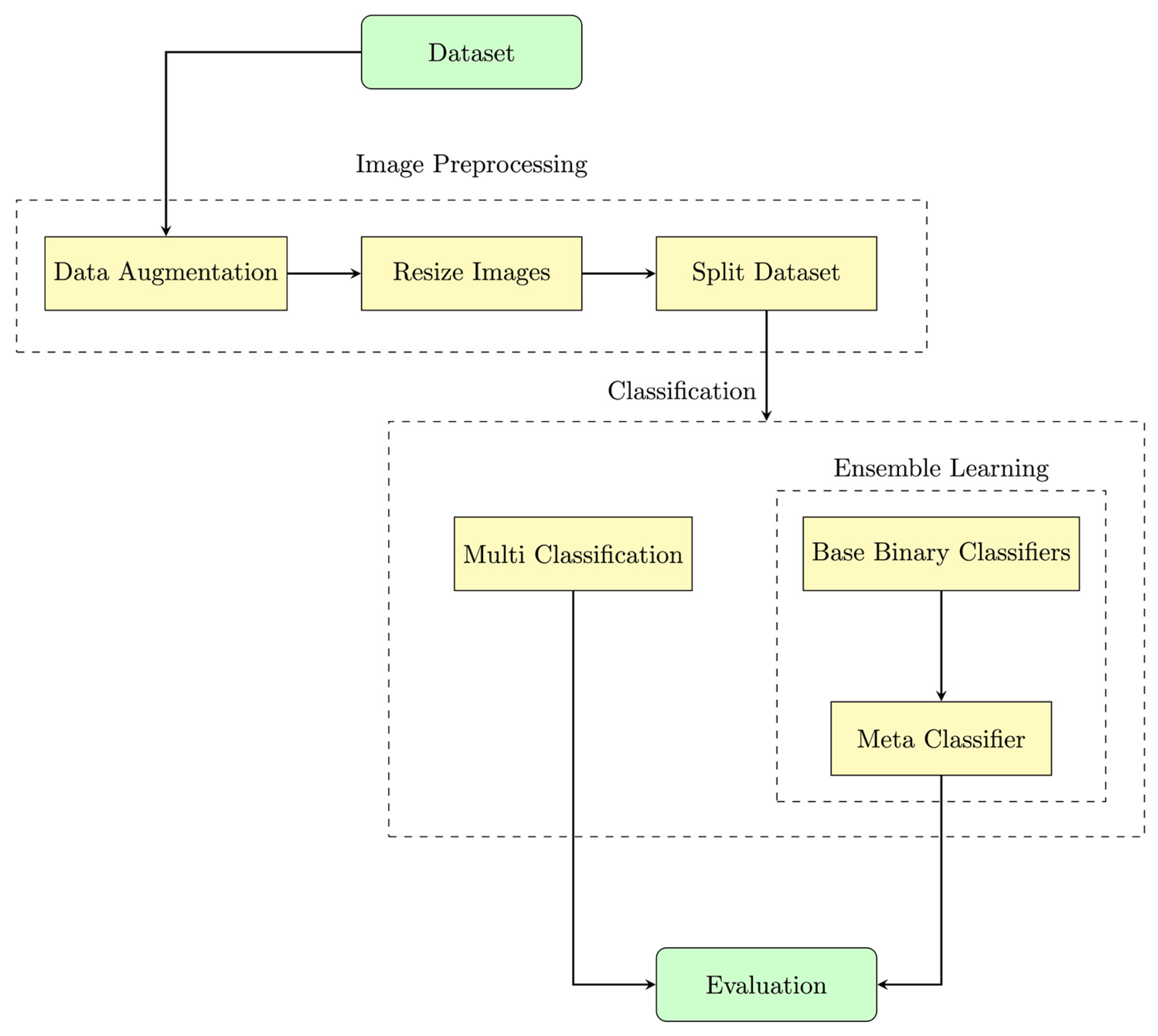
The primary goal of this paper is to advance FER by classifying facial images based on emotions, utilizing the high-performing EfficientNet model. This choice is motivated by its strong predictive performance and high computational efficiency [16,77,78,79,80,81,82] on small datasets, in addition to the relatively low number of parameters, which reduces the risk of overfitting. Our methodology endeavors to achieve highly accurate and efficient emotion classification from facial expressions, thereby making significant contributions to the fields of computer vision and affective computing. The sequential steps of the proposed solution are illustrated in Figure 5. The methodology comprises three main steps: data preprocessing; classification, conducted as two distinct experiments (multiclass classification and ensemble learning); and the final evaluation.
The results in this paper were derived from a series of experiments, which we summarize in terms of two experiments. The first experiment was conducted as a multiclass classification problem, employing the EfficientNet-B0 model with data augmentation. In the second experiment, we adopted the one-versus-rest (OvR) classification strategy, employing binary classifiers, and incorporated a stacking technique, also referred to as stacked generalization or stacked ensembles, to enhance the performance (the meta-classifier). We will start by explaining the aforementioned techniques in general; then, we will delve into the methodology in more detail.
Multiclass Classification: This is a technique that aims to classify instances into one of multiple classes. Each new instance point can be assigned only to one class [83]. Models designed for multiclass classification can handle multiple classes directly—for example, random forests, SVM, and neural networks such as CNN models like EfficientNet-B0. The output of a multiclass classifier is a single prediction indicating the most likely class for a given instance.
OvR Classification Strategy: This is a technique used to extend binary classification algorithms to handle multiclass problems. For each class, a binary classifier is trained to distinguish instances of that class from instances of all other classes combined [83]. Thus, the number of binary classifiers is equal to the number of classes in the dataset. The benefit of OvR classification is that it effectively decomposes the multiclass problem into multiple binary classification sub-problems.
Stacking: This is an ensemble learning strategy in machine learning (ML) that combines the predictions of multiple base models to achieve improved overall performance in the final prediction. The main goal of stacking is to obtain better performance based on various predictions with high accuracy, rather than relying on a single model [84].
Meta-Classifier Model: Meta-learning is an ML method that utilizes the predictions of other ML algorithms as part of the learning process [85]. The meta-classifier is based on the ensemble method, i.e., stacking [86]. The concept of stacking ensemble learning is implemented in three stages: first, the base classifiers are trained on binary datasets from the initial training set; second, predictions are generated on the validation set by each binary classifier (base classifiers); third, the final prediction of the meta-classifier is performed based on the predictions of the base classifiers on the validation set. The meta-classifier is trained and tested based on these validation sets from the binary classifiers [87]. The advantages of stacking include the following [84]:
  • Improved Predictive Performance: This is achieved by combining the strengths of multiple models.
  • Model Diversity: This is achieved by using various base models at the same time and then combining their predictions.
  • Reduced Overfitting: It generalizes better to unseen data.
  • Flexibility: It can accommodate various types of models and algorithms.
  • Ensemble Learning: Ensemble methods often outperform individual models.
  • Adaptability: It can be adapted to different types of ML tasks, including classification, regression, and clustering. It can also be extended to handle more complex scenarios, such as multiclass classification.

4.1. Dataset

We utilized a dataset containing a diverse range of natural human facial images for emotion recognition, sourced from the internet and manually annotated on Kaggle.com [88]. This dataset was titled “Natural Human Face Images for Emotion Recognition” (NHFIER) [89,90]. It contains over 5500 images sorted into eight different facial expression classes: 890 for anger, 208 for contempt, 439 for disgust, 570 for fear, 1406 for happiness, 524 for neutrality, 746 for sadness, and 775 for surprise. All images are represented as grayscale human faces (or sketches) with a resolution of 224 × 224 pixels, stored in PNG format [89,90].

4.2. Data Preprocessing

This section describes the preprocessing steps prior to the classification process, i.e., where images were ensured to be of a specific size. Moreover, it discusses the data augmentation process, where variation in the images was ensured to mitigate the problem of dataset imbalance. Furthermore, it explains the dataset splitting process.

4.2.1. Image Resizing

In this step, the images of the dataset were resized to the input size expected by the EfficientNet-B0 model. EfficientNet-B0 requires input images of size (224, 224, 3) [91].

4.2.2. Data Augmentation

Data augmentation refers to a set of techniques used in ML models to increase the diversity and size of the training data by creating slightly modified copies of the existing data or generating new versions of the data [92]. Data augmentation includes techniques such as random rotation, flipping, and shifts. It aims to enhance model generalization and reduce overfitting [92]. We applied this augmentation step on the dataset to augment it with additional instances for both experiments. We limited the augmentation process on our dataset to the following techniques, which we believed would not adversely affect the recognition of facial emotions: rotation between −10° and +10°; grayscale applied to 15% of the images; and brightness between −15% and +15%. A slight rotation between −10° and +10° simulates natural head tilts, brightness adjustments between −15% and +15% simulate lighting variations, and converting 15% of the images to grayscale introduces additional variability by reducing the reliance on color cues. We avoided using other techniques, such as rotation with large angles, flips, and shifting, because these techniques might affect important facial features and the positions of the facial landmarks (i.e., eyes, mouth, etc.). The transformation process was implemented with the use of Roboflow [93]. The total number of instances in the dataset after augmentation was 11,112 across the eight classes.

4.2.3. Balancing the Dataset

Balancing a dataset refers to the process of ensuring that each class in the dataset has approximately the same number of instances. Balancing the dataset is important in ML tasks, especially for classification problems, as it helps to avoid biases towards a particular class. Consequently, a positive effect on the model performance might be observed. We applied the oversampling technique to a obtain balanced dataset in the second experiment. Further details are discussed later in Section 5.3.

4.2.4. Splitting the Dataset

Data splitting is a compulsory and essential step in ML and DL research. Usually, the splitting process involves creating two or three distinct subsets of the main dataset to perform different functions during model development [94]. The typical splits in supervised ML tasks include three randomly partitioned sets, as follows [94]:
Training Set: This subset is the largest part of the dataset and is used to train the model on the patterns and relationships within the data.
Validation Set: This is an independent dataset for the fine-tuning of the model’s parameters and its evaluation after training to assess the performance of the model and prevent overfitting.
Test Set: This last set contains unseen data by the model and is used to check the final accuracy. It provides an unbiased evaluation of the model’s performance on new, unseen data.
As we conducted two experiments, we employed one data split for both experiments: 70% for training data, 15% for validation data, and 15% for test data. The details of this split are summarized in Table 3. The second experiment involved multiple classifiers, namely eight binary classifiers and one meta-classifier, all of which used the same data split, i.e., 70% for training, 15% for validation, and 15% for testing, as shown in Table 3.

4.3. Model Architecture

In both the multiclass classification and ensemble learning experiments, we utilized EfficientNet-B0 as the foundational model. Initializing the model with pretrained weights from ImageNet facilitated the capture of high-level features. Subsequently, we applied a fine-tuning process, which was as follows.
We generated the model with num_neurons = 16. The input layer was defined with a shape of (224, 224, 3), which corresponded to the dimensions of the input images. The parameter include_top was set to False to exclude the final fully connected layers, as well as weights = ‘imagenet’. The output of the base EfficientNet-B0 model was propagated through a GAP layer to reduce the spatial dimensions of the feature maps. A dropout layer with a dropout rate of 0.5 was applied to reduce overfitting. Then, a fully connected dense layer with ReLU activation and a number of neurons = 16 was added. After this, batch normalization was applied to normalize the activations of the previous layer. Then, another dropout layer with a dropout rate of 0.5 was added for additional regularization. Then, for multiclass classification, a final output layer with eight neurons was added with SoftMax to produce a probability distribution over the classes; meanwhile, for binary classifiers in the ensemble learning experiments, a dense layer with a single neuron and sigmoid activation was added to produce the model’s output for binary classification. We also unfroze the last 20 layers of the base EfficientNet-B0 to allow fine-tuning, while the earlier layers remained frozen to retain general ImageNet features.
The parameters used for model configuration in both experiments are summarized in Table 4, which presents a side-by-side comparison of the configurations used in the multiclass and binary classification models. Both models are based on EfficientNet-B0 as the base architecture but differ in terms of their specific configurations, being tailored to either multiclass or binary outputs. As shown in Table 4, the differences between the two models lie in the number of output-dense units and the activation function, as detailed in Table 4.

4.4. Model Training

After initializing the model with pretrained ImageNet weights, the model was compiled as follows. In the multiclass classification experiment, an appropriate loss function was selected (sparse_categorical_crossentropy), which was used for integer labels; the Adam optimizer was used; and the learning rate was set to 1 × 10⁻³. An accuracy metric was used for evaluation. On the other hand, in the ensemble learning approach, an appropriate loss function was selected (binary_crossentropy), which was suitable for binary classification; the Adam optimizer was employed; and the learning rate was set to 1 × 10⁻³. An accuracy metric was used for evaluation.

4.5. Model Evaluation

In both experiments, we conducted evaluations on the test set to assess the model’s performance. Subsequently, we analyzed the performance metrics, including the accuracy, confusion matrices, precision, recall, and F1-score. In both experiments, during model generation, hyperparameter tuning was performed with different values for parameters such as the learning rate, batch size, number of epochs, dropout layers, and dropout rate, seeking to select the best combination of hyperparameters and maximize the model’s performance on the validation set.

5. Experiment

The main aim of this work was to classify facial images based on emotions to advance FER by leveraging the high-performing EfficientNet model and stacking techniques. This section provides detailed insights into the two experiments conducted to classify emotions based on the facial images in the dataset.

5.1. Tools

A variety of tools and libraries were utilized as a part of this study, including python [95], the scikit-learn library (version 1.7.1) [96], TensorFlow (version 2.19.0) [97], Keras [98,99], NumPy (version 2.3.2) [100], Matplotlib (version 3.10.5) [101], seaborn (version 0.13.2) [102], and Google Colab [17].

5.2. Performance Measures

Performance measures are crucial in evaluating the effectiveness of developed models. The following are some common performance measures that were used in our experiments.
Average Accuracy for Multiclass Classification: The accuracy measure calculates the overall correctness across multiple classes. The formula for calculating the accuracy is as follows:
A v e r a g e   A c c u r a c y = 1 N i = 1 N t p i + t n i t p i + f n i + f p i + t n i
where N refers to the number of classes; t p i , or true positives, refers to the number of instances correctly predicted as class i; t n i , or true negatives, refers to the number of instances correctly predicted as not class i; f p i , or false positives, refers to the number of instances incorrectly assigned to class i; and f n i , or false negatives, represents the number of instances that are not recognized as class instances. Similarly, for binary classification, accuracy reflects the overall effectiveness of a classifier [103]:
A c c u r a c y = t p + t n t p + f n + f p + t n
Confusion Matrix: A confusion matrix is a table that provides a detailed summary of a model’s performance, including the number of true positive (TP), true negative (TN), false positive (FP), and false negative (FN) predictions for each class. For multiclass classification, the confusion matrix extends to multiple classes, with each row and column corresponding to a specific class. The rows in the confusion matrix represent the original class distribution, while the columns represent the predicted distribution by the classifier [104,105].
F1-Score: This is the harmonic mean of the precision and recall for a specific class. It provides a balanced measure that considers both precision and recall [106]. The formula used to calculate the F1-score is included below.
P r e c i s i o n = T P ( T P + F P )
R e c a l l = T P ( T P + F N )
F 1 = 2 × P r e c i s i o n × R e c a l l ( P r e c i s i o n + R e c a l l )

5.3. Experimental Settings

This section details the experimental setup and parameters, explaining how the experiments were conducted.

5.3.1. Multiclass Classification Experiment

Initially, the dataset contained varying instances across classes: 890 in anger, 208 in contempt, 439 in disgust, 570 in fear, 1406 in happiness, 524 in neutrality, 746 in sadness, and 775 in surprise. We augmented the dataset by creating synthetic variations of the images, as discussed in Section 4.2.2; then, the total number of instances after augmentation in the dataset was 11,112 across the eight classes. Subsequently, we preprocessed the dataset by resizing the images and transforming the categorical labels into integer labels. We applied EfficientNet normalization. Then, the preprocessed image and its corresponding label were added to the lists and converted into NumPy arrays, which were required for training.
Data shuffling was performed to randomize both the images and their corresponding labels before splitting the dataset. The dataset was divided into training, validation, and test subsets, with 70% allocated for training, 15% for validation, and 15% for testing. The initial learning rate was set to 0.001, with 100 epochs and a batch size of 32. During the training process, we monitored the progress using three callback classes from Keras: ModelCheckpoint, EarlyStopping, and ReduceLROnPlateau. These standard techniques are employed in DL to save model weights, halt training if performance stagnates, and adjust the learning rates during training, respectively [107,108,109]. ModelCheckpoint saves the models weights to a file when the validation accuracy improves. EarlyStopping stops the training when the validation accuracy does not improve for a specified number of epochs. ReduceLROnPlateau adjusts the learning rate when the validation accuracy plateaus, reducing the learning rate by a factor of 0.2 if no improvement is observed for a specified number of epochs, min_lr = 1 × 10⁻¹⁵.

5.3.2. Ensemble Learning Approach

The idea for the second experiment arose as we sought to divide the main and complex problems into smaller and simpler sub-problems. Finding solutions for each sub-problem was expected to lead to finding a solution for the main, complex problem. Therefore, we started by dividing the augmented dataset into eight binary datasets that corresponded to the eight facial emotions. Then, we generated eight binary classifiers, where each binary classifier was tasked with predicting a specific facial emotion; for example, the “happy” binary classifier predicts whether the facial emotion can be classified as a happy emotion or not. Finally, we used the technique of stacking to generate a meta-classifier that combined the aforementioned eight binary classifiers in order to predict the correct facial emotion.
We used the augmented dataset that contained 11,112 instances across eight categories. Then, we converted this dataset into eight binary datasets using the OvR strategy. Each binary dataset consisted of two classes: a negative class, which included all instances from the other emotion categories, and a positive class, which comprised instances belonging to the target emotion. The positive class was constructed by selecting the same number of original instances as in the target class from the augmented dataset. To address class imbalance, we applied random oversampling to the positive class, increasing its size to match that of the negative class. The final class distributions for each binary classifier are presented in Table 5. We preprocessed the datasets following the same procedure as in the multiclass classification experiment. Data shuffling was performed to shuffle both the images and their corresponding labels to ensure that the data were randomly ordered before splitting. The dataset was divided into training, validation, and test sets (70% for the training set, 15% for the validation set, and 15% for testing set). The initial learning rate was 0.001. The number of epochs was 100, and the batch size was 32. During the training process, we monitored the progress using three callback classes from Keras: ModelCheckpoint, EarlyStopping, and ReduceLROnPlateau [107,108,109]. ModelCheckpoint saves the models weights to a file when the validation accuracy improves. EarlyStopping stops the training when the validation accuracy does not improve for a specified number of epochs (patience = 5). ReduceLROnPlateau adjusts the learning rate when the validation accuracy plateaus, reducing the learning rate by a factor of 0.2 if no improvement is observed for a specified number of epochs (min_lr = 1 × 10⁻¹⁵).

5.3.3. Implementation of the Meta-Classifier

The meta-classifier was employed using the RF classifier as follows. We generated eight binary models, where each model corresponded to a specific facial emotion. Then, the meta-classifier aggregated the predications of the binary classifiers. In order to train the meta-classifier, the entire test datasets of the binary classifiers were utilized as the test set, comprising unseen images, to train, validate, and test the meta-classifier. We shuffled the test datasets to ensure randomness in the split. The shuffled test datasets were split into 70% for training, 15% for validation, and 15% for testing. Next, a stacking approach was implemented. We utilized the pretrained binary classifiers to extract features from the training set. The RF classifier was initialized and trained on the extracted features from the eight binary classifiers to combine the binary outputs into a final multiclass prediction. The meta-classifier was validated on the validation set using the trained meta-classifier. Finally, we tested the meta-classifier on the test set to measure its generalization performance. For the RF classifier, we utilized two parameters, namely n_estimators = 100 decision trees and random_state = 42, which proved to be the optimal choices for our experiment.

6. Results and Analysis

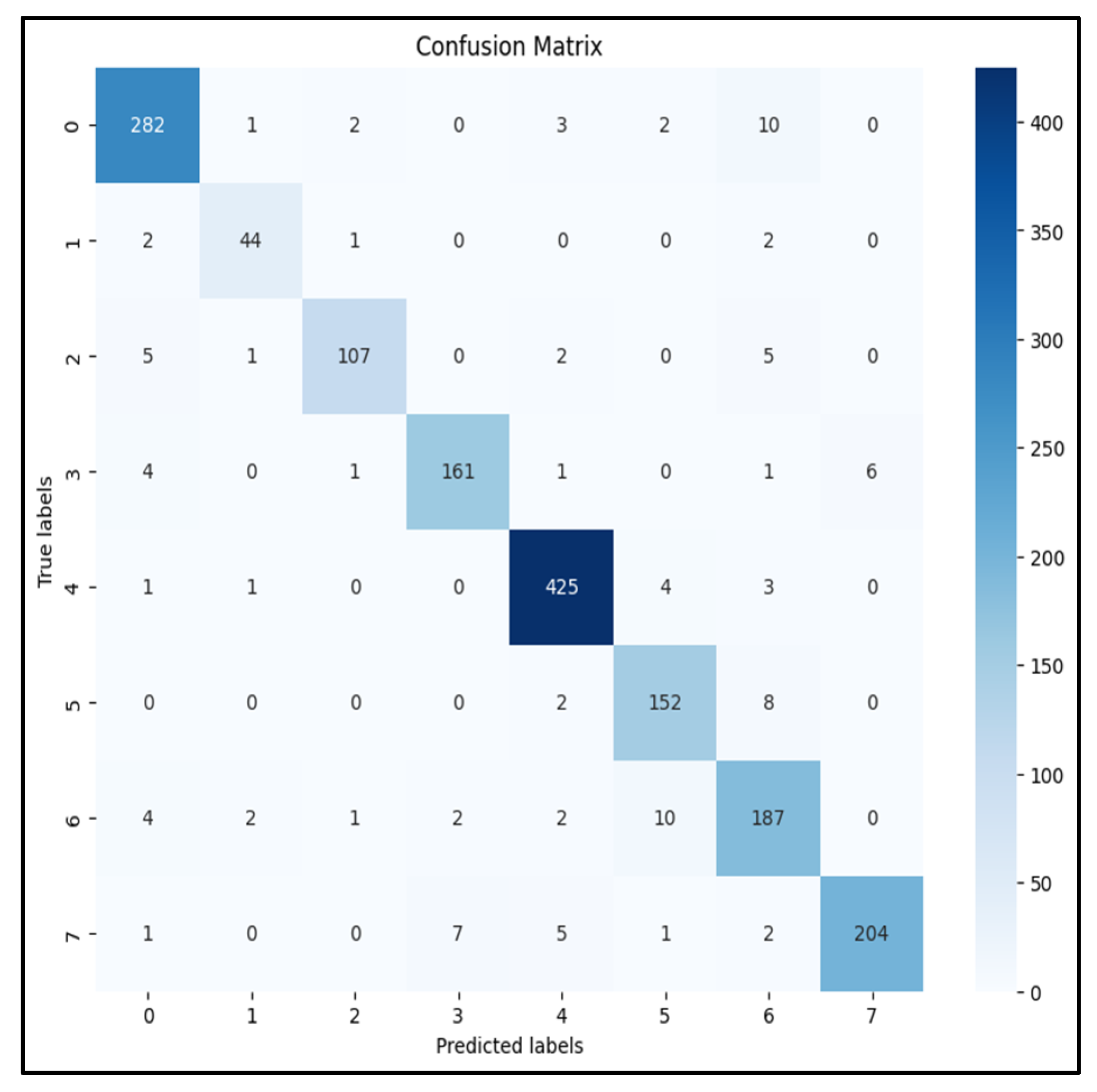
Multiclass Classification Experiment: We achieved training accuracy of 99%, with validation accuracy of 94%, while the test accuracy was 94%. Figure 6 illustrates the confusion matrix for the first experiment, where darker colors indicate higher accuracy. Numeric labels were assigned as follows: 0 = anger class; 1= contempt class; 2= disgust class; 3 = fear class; 4 = happy class; 5 = neutral class; 6 = sad class; and 7 = surprise class.
The confusion matrix from Figure 6 reveals varying levels of classification performance across the emotion classes. Class 0 (anger) had the highest number of misclassifications, with 10 instances mislabeled as sad. Moreover, Class 6 (sad) had 10 instances mislabeled as neutral. The remaining classes were classified well. Overall, the most frequent misclassifications occurred between semantically or visually similar expressions, such as anger–sad and sad–neutral, which have overlapping facial features—this makes these pairs particularly challenging for the model to distinguish.
To enhance the results, in the second experiment, we explored another strategy as an alternative approach to address the complexity of the model and the unique characteristics of the dataset.
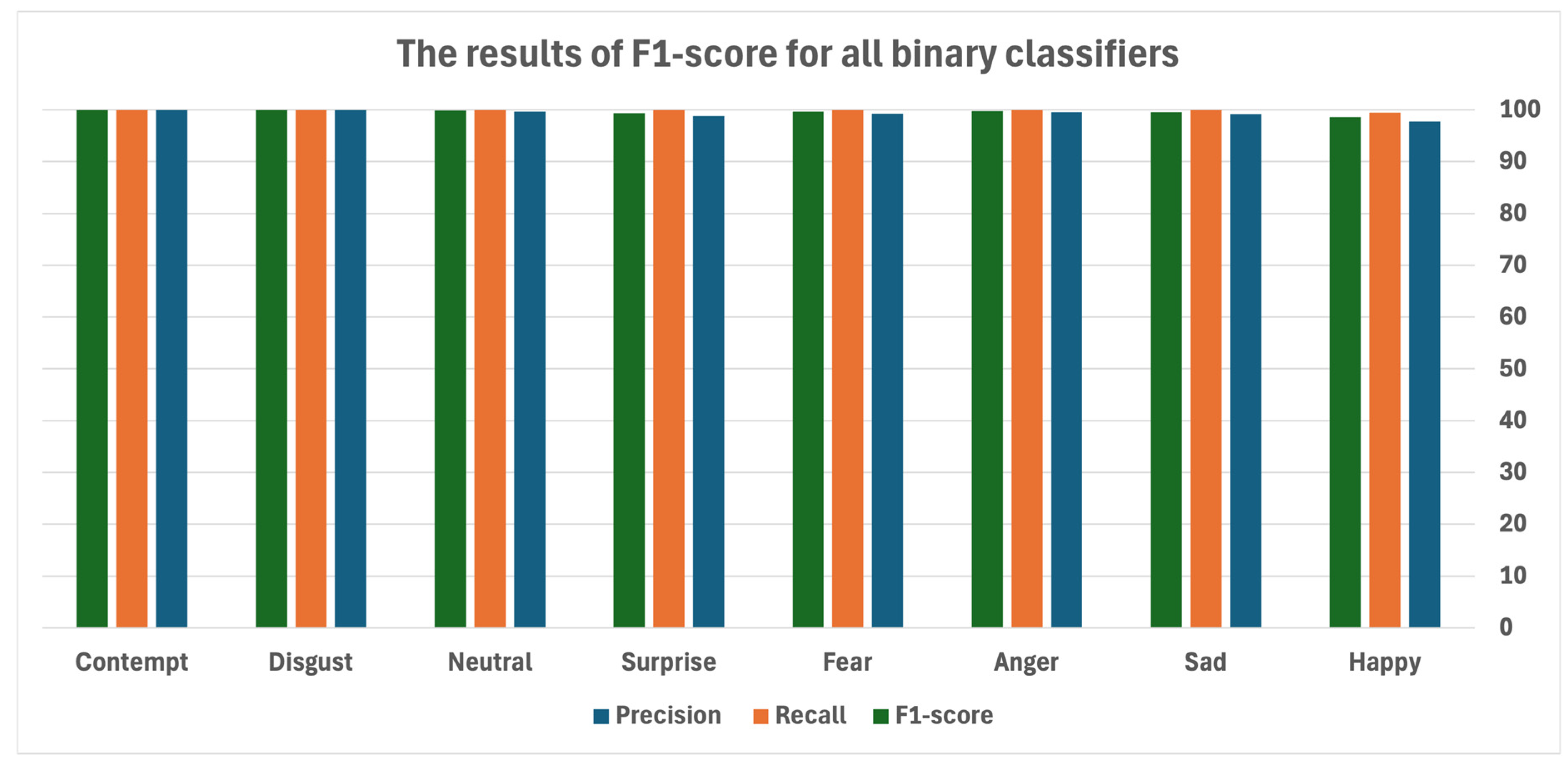
Ensemble Learning Experiment: After conducting the second experiment, we achieved high accuracies for training, validation, and testing—all around 99% across all binary classifiers, as indicated in Table 6 and Figure 7. This marked the initial step towards enhancing our results.
Most of the binary classifiers stopped at epochs 19–20 due to the early stopping mechanism implemented using the EarlyStopping callback, since there was no improvement observed in the validation accuracy metric within the specified patience period. Table 7 summarizes the F1-score results for all binary classifiers, derived from their respective test sets. The F1-score exceeds 98% for all binary classifiers, as shown in Figure 8, signifying a remarkable level of accuracy and completeness in their predictions. This suggests a commendable balance between the precision and recall values within the binary models.
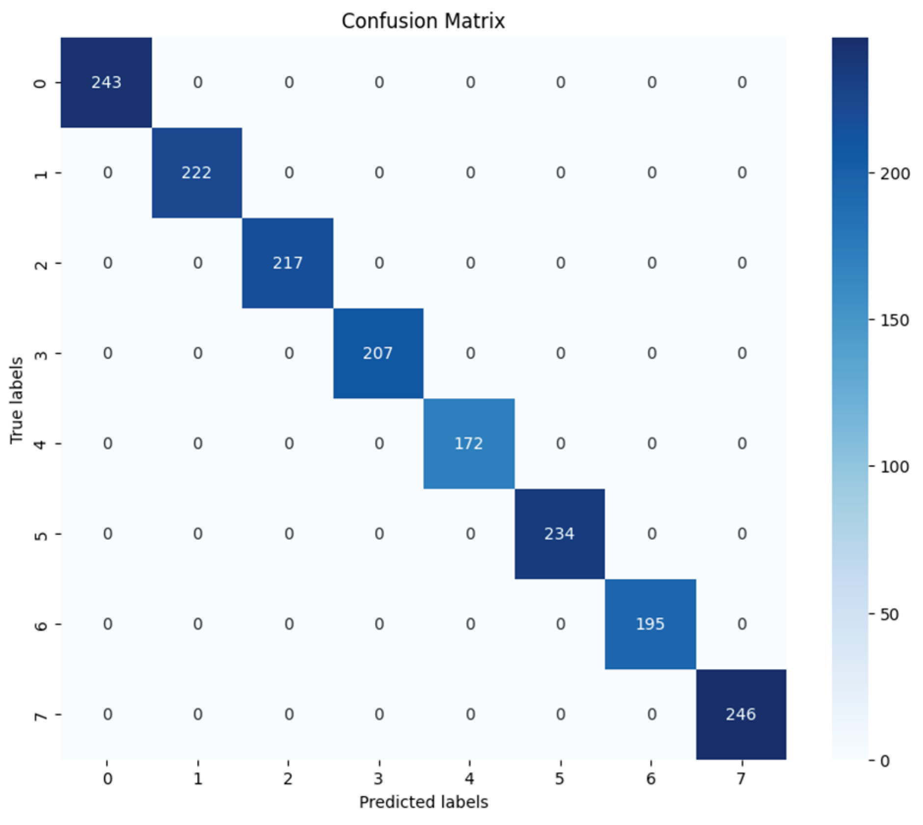
When the meta-classifier was utilized following the ensemble learning approach, accuracy of 100% was achieved on both the validation and test sets, which represents a significant improvement compared to the first experiment. This indicates that both the binary classifiers and meta-classifiers were highly effective in classifying facial emotions. Figure 9 illustrates the confusion matrix for the second experiment, where darker colors represent higher accuracy. Numeric labels were assigned as follows: 0 = anger class; 1 = contempt class; 2 = disgust class; 3 = fear class; 4 = happy class; 5 = neutral class; 6 = sad class; and 7 = surprise class. The meta-classifier model also achieved 100% precision, 100% recall, and an F1-score of 100%. Figure 7 demonstrates its strong classification performance across all eight emotion classes, which contrasts with the confusion matrix shown in Figure 6. This comparison highlights a significant improvement in classification accuracy and superior performance when using an ensemble learning approach as opposed to relying on a single, complex, multiclass classifier.
The proposed solution overcomes the problems of inaccurate detections and predictions of diverse facial emotions. It must be noted that various obstacles in facial expression detection, such as variations in lighting conditions, occlusion, random brightness, non-frontal faces, glasses, hats, and diversity in facial features among individuals, might have a negative impact on the model performance. We also noticed similarities between some classes—for example, the contempt and anger classes. Additionally, most of the FER datasets employed in related studies contain only seven classes, excluding the contempt class. Therefore, including the contempt class added an additional challenge in terms of the number of classes under consideration and in terms of balancing, as the contempt class was the only class with fewer instances in the original dataset.
Additional Testing of the Meta-Classifier
We further tested our meta-classifier under the same settings. As for the second experiment, we used the RF ML classifier based on the predictions of the eight binary models to train, validate, and test the meta-classifier on a new dataset that was not seen by the eight binary classifiers. We utilized the Extended CK+ dataset [110], which contains a total of 981 images in PNG format. This dataset includes seven classes of emotions: anger, contempt, disgust, fear, happiness, sadness, and surprise. We preprocessed the dataset following the same procedure as that undertaken for the binary classifiers. Subsequently, we shuffled it to ensure a random split. The initial split was 70% for the training set and 30% for the evaluation set; then, we further divided the evaluation set into 15% for the validation set and 15% for the testing set. Then, a stacking approach was deployed, following the same approach as used in the second experiment with ensemble learning. We utilized the pretrained binary classifiers to extract features from the training set and to obtain predictions on the training, validation, and testing sets. The meta-classifier was an RF classifier tuned with two parameters: n_estimators = 100 decision trees and random_state = 42. It was evaluated on the validation and testing sets. The results of this evaluation indicated accuracy of 90% on the validation set and 92% on the test set. A precision score of 93 was achieved, along with recall of 92% and an F1-score of 92%. These results demonstrate the effectiveness of applying transfer learning and stacking techniques with EfficientNet-B0 for FER tasks.

7. Conclusions and Future Work

In conclusion, this paper delineates a promising avenue to advance the field of FER through the utilization of the EfficientNet-B0 architecture and the concept of stacking. Eight classes of facial emotions were predicted in this study. The present work combined transfer learning from a pretrained model on the ImageNet dataset, tuning strategies, and binary and meta-classifiers. The experiment decomposed the multiclass problem into multiple binary classification sub-problems through the OvR classification strategy; then, the stacking technique was utilized to create a meta-classifier to predict facial emotions based on natural face images. By harnessing the efficiency and effectiveness of the EfficientNet-B0 model, we effectively addressed the issue of inaccurate detections and predictions across diverse facial emotions. The proposed approach has significant potential to enhance the accuracy and generalization capabilities of FER models, thereby contributing to more reliable and applicable solutions in real-world scenarios. The proposed approach achieved 100% and 92% classification accuracy in facial emotion recognition on the test sets obtained from the meta-classifiers. The experimental results underscore the strength of EfficientNet-B0, achieved via the meticulous exploration of its capabilities, and we expect this study to make a notable contribution to the broader landscape of emotion recognition research. In the future, this work will be extended with larger datasets encompassing more diverse, multi-modal data—for example, classifying facial emotions while considering both facial expressions and voice tune. Furthermore, a variety of DL techniques will be utilized for FER, and their performance will be evaluated.

Author Contributions

Conceptualization, M.A. and F.A.A.; Data curation, M.A.; Formal analysis, M.A. and F.A.A.; Investigation, M.A.; Methodology, M.A. and F.A.A.; Project administration, F.A.A.; Resources, M.A. and F.A.A.; Software, M.A.; Supervision, F.A.A.; Validation, M.A. and F.A.A.; Visualization, M.A.; Writing—original draft, M.A.; Writing—review and editing, M.A. and F.A.A. All authors have read and agreed to the published version of the manuscript.

Funding

This research was funded by King Saud University, Riyadh, Saudi Arabia, through the Ongoing Research Funding Program, (ORFFT-2025-033-1), King Saud University, Riyadh, Saudi Arabia.

Data Availability Statement

The authors utilized publicly available datasets from https://www.kaggle.com/datasets/sudarshanvaidya/random-images-for-face-emotion-recognition (accessed on 7 July 2024) and https://www.kaggle.com/datasets/shuvoalok/ck-dataset/data (accessed on 7 July 2024). The original contributions presented in this study are included in the article. Further inquiries can be directed to the corresponding author.

Acknowledgments

The authors would like to thank Ongoing Research Funding Program, (ORFFT-2025-033-1), King Saud University, Riyadh, Saudi Arabia for financial support.

Conflicts of Interest

The authors declare that they have no known competing financial interests or personal relationships that could have appeared to influence the work reported in this paper.

Abbreviations

The following abbreviations are used in this manuscript:
FERFacial Emotion Recognition
NHFIERNatural Human Face Images for Emotion Recognition
CK+Cohn–Kanade
DLDeep Learning
MLMachine Learning
SVMSupport Vector Machine
k-NNk-Nearest Neighbors
CNNsConvolutional Neural Networks
RNNsRecurrent Neural Networks
FACSFacial Action Coding System
AUsAction Units
LBPLocal Binary Pattern
DTDecision Tree
RFRandom Forest
MLPMultilayer Perceptron
dDepth
wWidth
rResolution
AdaBoostAdaptive Boosting
SGBStochastic Gradient Boosting
XGBoostExtreme Gradient Boosting
AIArtificial Intelligence
FACFacial Action Unit
LDPLocal Directional Pattern
HoGHistogram of Oriented Gradients
ReLURectified Linear Unit
AAMActive Appearance Model
SDMSupervised Descent Method
DISFADenver Intensity of Spontaneous Facial Actions
FERCFacial Emotion Recognition Using Convolutional Neural Networks
SGDStochastic Gradient Descent
VGG-16Visual Geometry Group-16
GAPGlobal Average Pooling
RAF-DBReal-World Affective Faces
AR-TE-CATFFNetAttention-Rectified and Texture-Enhanced Cross-Attention Transformer Feature Fusion Network
PCAPrincipal Component Analysis
LDALinear Discriminant Analysis
OvROne-versus-Rest
TPTrue Positive
TNTrue Negative
FPFalse Positive
FNFalse Negative

References

  1. Mehrabian, A. Nonverbal Communication; Aldine Transaction: New Brunswick, NJ, USA, 2007. [Google Scholar]
  2. Liliana, D.Y. Emotion recognition from facial expression using deep convolutional neural network. J. Phys. Conf. Ser. 2019, 1193, 012004. [Google Scholar] [CrossRef]
  3. Mollahosseini, A.; Chan, D.; Mahoor, M.H. Going deeper in facial expression recognition using deep neural networks. In Proceedings of the IEEE Winter Conference on Applications of Computer Vision (WACV), Lake Placid, NY, USA, 7–10 March 2016; pp. 1–10. [Google Scholar] [CrossRef]
  4. Paweł, T.; Marcin, K.; Andrzej, M.; Remigiusz, R. Emotion recognition using facial expressions. Procedia Comput. Sci. 2017, 108, 1175–1184. [Google Scholar] [CrossRef]
  5. Mehendale, N. Facial emotion recognition using convolutional neural networks (FERC). SN Appl. Sci. 2020, 2, 446. [Google Scholar] [CrossRef]
  6. Agrawal, A.; Mittal, N. Using CNN for facial expression recognition: A study of the effects of kernel size and number of filters on accuracy. Vis. Comput. 2020, 36, 405–412. [Google Scholar] [CrossRef]
  7. Ahmed, T.U.; Hossain, S.; Hossain, M.S.; ul islam, R.; Andersson, K. Facial Expression Recognition using Convolutional Neural Network with Data Augmentation. In Proceedings of the Joint 8th International Conference on Informatics, Electronics & Vision (ICIEV) and 2019 3rd International Conference on Imaging, Vision & Pattern Recognition (icIVPR), Spokane, WA, USA, 30 May–2 June 2019; pp. 336–341. [Google Scholar] [CrossRef]
  8. Kusuma, G.P.; Jonathan, J.; Andreas, L. Emotion Recognition on FER-2013 Face Images Using Fine-Tuned VGG-16. Adv. Sci. Technol. Eng. Syst. J. 2020, 5, 315–322. [Google Scholar] [CrossRef]
  9. Singh, R.; Sharma, H.; Mehta, N.K.; Vohra, A.; Singh, S. EfficientNet For Human Fer Using Transfer Learning. ICTACT J. Soft Comput. 2022, 13, 2792–2797. [Google Scholar] [CrossRef]
  10. Lawpanom, R.; Songpan, W.; Kaewyotha, J. Advancing Facial Expression Recognition in Online Learning Education Using a Homogeneous Ensemble CNN Approach. Appl. Sci. 2024, 14, 1156. [Google Scholar] [CrossRef]
  11. Talele, M.; Jain, R. A Comparative Analysis of CNNs and ResNet50 for Facial Emotion Recognition. Eng. Technol. Appl. Sci. Res. 2025, 15, 20693–20701. [Google Scholar] [CrossRef]
  12. Sun, M.; Cui, W.; Zhang, Y.; Yu, S.; Liao, X.; Hu, B.; Li, Y. Attention-Rectified and Texture-Enhanced Cross-Attention Transformer Feature Fusion Network for Facial Expression Recognition. IEEE Trans. Ind. Inform. 2023, 19, 11823–11832. [Google Scholar] [CrossRef]
  13. Wasi, A.T.; Šerbetar, K.; Islam, R.; Rafi, T.; Chae, D.-K. ARBEx: Attentive feature extraction with reliability balancing for robust facial expression learning. arXiv 2023. [Google Scholar] [CrossRef]
  14. El Aroussi, M.; El Hassouni, M.; Ghouzali, S.; Rziza, M.; Aboutajdine, D. Local appearance-based face recognition method using block-based steerable pyramid transform. Signal Process. 2011, 91, 38–50. [Google Scholar] [CrossRef]
  15. Fakhar, K.; El Aroussi, M.; Saadane, R.; Wahbi, M.; Aboutajdine, D. Fusion of face and iris features extraction based on steerable pyramid representation for multimodal biometrics. In Proceedings of the 2011 International Conference on Multimedia Computing and Systems, Ouarzazate, Morocco, 7–9 April 2011; pp. 1–4. [Google Scholar] [CrossRef]
  16. Tan, M.; Le, Q.V. EfficientNet: Rethinking Model Scaling for Convolutional Neural Networks. arXiv 2019, arXiv:1905.11946. [Google Scholar]
  17. “Google Colaboratory”, Google. Available online: https://colab.google/ (accessed on 7 May 2024).
  18. Safonova, A.; Ghazaryan, G.; Stiller, S.; Main-Knorn, M.; Nendel, C.; Ryo, M. Ten deep learning techniques to address small data problems with remote sensing. Int. J. Appl. Earth Obs. Geoinf. 2023, 125, 2023. [Google Scholar]
  19. Ekman, P.; Friesen, W.V. Constants across cultures in the face and emotion. J. Personal. Soc. Psychol. 1971, 17, 124–129. [Google Scholar] [CrossRef]
  20. Helkar, Y.; Sayyad, A.; Patil, P.G. Facial Emotion Recognition System (FERS) Using Machine Learning. Int. J. Innov. Res. Sci. Eng. Technol. 2023, 12, 7781–7786. [Google Scholar]
  21. Mellouk, W.; Wahida, H. Facial emotion recognition using deep learning: Review and insights. Procedia Comput. Sci. 2020, 175, 689–694. [Google Scholar] [CrossRef]
  22. EIA Group. Facial Action Coding System (FACS). 2022. Available online: https://www.eiagroup.com/resources/facial-expressions/facial-action-coding-system-facs/ (accessed on 7 May 2024).
  23. Ming, Z.; Bugeau, A.; Rouas, J.; Shochi, T. Facial Action Units intensity estimation by the fusion of features with multi-kernel Support Vector Machine. In Proceedings of the 2015 11th IEEE International Conference and Workshops on Automatic Face and Gesture Recognition (FG), Ljubljana, Slovenia, 4–8 May 2015; Volume 6, pp. 1–6. [Google Scholar]
  24. Gudi, A.; Tasli, H.E.; Den Uyl, T.M.; Maroulis, A. Deep Learning based FACS Action Unit Occurrence and Intensity Estimation. In Proceedings of the 2015 11th IEEE International Conference and Workshops on Automatic Face and Gesture Recognition (FG), Ljubljana, Slovenia, 4–8 May 2015; pp. 1–5. [Google Scholar] [CrossRef]
  25. Smith, R.S.; Windeatt, T. Facial action unit recognition using multi-class classification. Neurocomputing 2015, 150, 440–448. [Google Scholar] [CrossRef]
  26. Taheri, S.; Qiu, Q.; Chellappa, R. Structure-preserving sparse decomposition for facial expression analysis. IEEE Trans. Image Process. Publ. IEEE Signal Process. Soc. 2014, 23, 3590–3603. [Google Scholar] [CrossRef]
  27. Valstar, M.F.; Almaev, T.; Girard, J.M.; McKeown, G.; Mehu, M.; Yin, L.; Pantic, M.; Cohn, J.F. FERA 2015—Second Facial Expression Recognition and Analysis Challenge. In Proceedings of the 11th IEEE International Conference and Workshops on Automatic Face and Gesture Recognition (FG), Ljubljana, Slovenia, 4–8 May 2015; Volume 6, pp. 1–8. [Google Scholar]
  28. Chu, W.S.; De la Torre, F.; Cohn, J.F. Learning Facial Action Units with Spatiotemporal Cues and Multi-label Sampling. Image Vis. Comput. 2019, 81, 1–14. [Google Scholar] [CrossRef] [PubMed] [PubMed Central]
  29. Bařina, D. Gabor Wavelets in Image Processing. In Proceedings of the 17th Conference STUDENT EEICT 2011, Brno, Czech Republic, 2011. [Google Scholar]
  30. Choi, W.P.; Tse, S.H.; Wong, K.W.; Lam, K.M. Simplified Gabor wavelets for human face recognition. Pattern Recognit. 2007, 41, 1186–1199. [Google Scholar] [CrossRef]
  31. Shan, C.; Gong, S.; Mcowan, P.W. Facial expression recognition based on Local Binary Patterns: A comprehensive study. Image Vis. Comput. 2009, 27, 803–816. [Google Scholar] [CrossRef]
  32. Niu, B.; Gao, Z.; Guo, B. Facial Expression Recognition with LBP and ORB Features. Comput. Intell. Neurosci. 2021, 2021, 8828245. [Google Scholar] [CrossRef] [PubMed] [PubMed Central]
  33. Sisquella Andrés, J. Machine Learning and Deep Learning for Emotion Recognition. Available online: https://upcommons.upc.edu/bitstream/handle/2117/184076/tfm-joan-sisquella.pdf?sequence=1 (accessed on 19 November 2023).
  34. Jain, V.; Aggarwal, P.; Kumar, T.; Taneja, V. Emotion Detection from Facial Expression using Support Vector Machine. Int. J. Comput. Appl. 2017, 167, 25–28. [Google Scholar] [CrossRef]
  35. Baeldung. Multiclass Classification Using Support Vector Machines. Baeldung on Computer Science. 2024. Available online: https://www.baeldung.com/cs/svm-multiclass-classification (accessed on 7 May 2024).
  36. Decision Tree. GeeksforGeeks. 2023. Available online: https://www.geeksforgeeks.org/decision-tree/ (accessed on 7 May 2024).
  37. What Is Random Forest? IBM. 2024. Available online: https://www.ibm.com/topics/random-forest (accessed on 7 May 2024).
  38. Ko, B.C. A Brief Review of Facial Emotion Recognition Based on Visual Information. Sensors 2018, 18, 401. [Google Scholar] [CrossRef] [PubMed]
  39. Kumar, D. Skip Connections & Resnet50. Medium. 2024. Available online: https://medium.com/@danushidk507/skip-connections-ab515d634e6d (accessed on 21 July 2024).
  40. Ioffe, S.; Szegedy, C. Batch normalization: Accelerating deep network training by reducing internal covariate shift. In Proceedings of the 32nd International Conference on International Conference on Machine Learning, Lille, France, 6–11 July 2015; pp. 448–456. [Google Scholar]
  41. Howard, A.G.; Zhu, M.; Chen, B.; Kalenichenko, D.; Wang, W.; Weyand, T.; Andreetto, M.; Adam, H. Mobilenets: Efficient convolutional neural networks for mobile vision applications. arXiv 2017, arXiv:1704.04861. [Google Scholar] [CrossRef]
  42. Sandler, M.; Howard, A.; Zhu, M.; Zhmoginov, A.; Chen, L.C. Mobilenetv2: Inverted residuals and linear bottlenecks. In Proceedings of the IEEE Conference on Computer Vision and Pattern Recognition, Salt Lake City, UT, USA, 18–23 June 2018. [Google Scholar]
  43. He, K.; Zhang, X.; Ren, S.; Sun, J. Deep residual learning for image recognition. In Proceedings of the IEEE Conference on Computer Vision and Pattern Recognition (CVPR), Las Vegas, NV, USA, 27–30 June 2016; pp. 770–778. [Google Scholar]
  44. Tan, M.; Chen, B.; Pang, R.; Vasudevan, V.; Sandler, M.; Howard, A.; Le, Q.V. MnasNet: Platform-aware neural architecture search for mobile. In Proceedings of the IEEE/CVF Conference on Computer Vision and Pattern Recognition (CVPR), Long Beach, CA, USA, 15–20 June 2019. [Google Scholar]
  45. Mohammed, A.; Kora, R. A comprehensive review on ensemble deep learning: Opportunities and challenges. J. King Saud Univ. Comput. Inf. Sci. 2023, 35, 757–774. [Google Scholar] [CrossRef]
  46. Odegua, R. An Empirical Study of Ensemble Techniques (Bagging, Boosting and Stacking). 2019. Available online: https://www.researchgate.net/publication/338681876_An_Empirical_Study_of_Ensemble_Techniques_Bagging_Boosting_and_Stacking (accessed on 7 May 2024).
  47. Mehrabian, A.; Ferris, S.R. Inference of attitudes from nonverbal communication in two channels. J. Consult. Psychol. 1967, 31, 248. [Google Scholar] [CrossRef]
  48. Samadiani, N.; Huang, G.; Cai, B.; Luo, W.; Chi, C.-H.; Xiang, Y.; He, J. A Review on Automatic Facial Expression Recognition Systems Assisted by Multimodal Sensor Data. Sensors 2019, 19, 1863. [Google Scholar] [CrossRef]
  49. Luma, A. Artificial Intelligence Tools for Facial Expression Analysis. 2021. Available online: https://www.researchgate.net/publication/354172772_Artificial_Intelligence_Tools_for_Facial_Expression_Analysis (accessed on 1 September 2024).
  50. Bhushan, S.C.; Babu, S.; Pushpendra, Y. Facial Expression Recognition. 2021. Available online: https://ssrn.com/abstract=3852666 (accessed on 7 May 2025). [CrossRef]
  51. Szegedy, C.; Liu, W.; Jia, Y.; Sermanet, P.; Reed, S.; Anguelov, D.; Erhan, D.; Vanhoucke, V.; Rabinovich, A. Going deeper with convolutions. In Proceedings of the 2015 IEEE Conference on Computer Vision and Pattern Recognition (CVPR), Boston, MA, USA, 7–12 June 2015; pp. 1–9. [Google Scholar]
  52. Pedraza, A.; Gallego, J.; Lopez, S.; Gonzalez, L.; Laurinavicius, A.; Bueno, G. Glomerulus Classification with Convolutional Neural Networks. In Medical Image Understanding and Analysis. MIUA 2017. Communications in Computer and Information Science; Valdés Hernández, M., González-Castro, V., Eds.; Springer: Cham, Switzerland, 2017; Volume 723. [Google Scholar] [CrossRef]
  53. Gross, R.; Matthews, I.; Cohn, J.; Kanade, T.; Baker, S. Multi-pie. Image Vis. Comput. 2010, 28, 807–813. [Google Scholar] [CrossRef]
  54. Pantic, M.; Valstar, M.; Rademaker, R.; Maat, L. Web-based database for facial expression analysis. In Proceedings of the IEEE International Conference on Multimedia and Expo, Amsterdam, The Netherlands, 6 July 2005; p. 5. [Google Scholar]
  55. Mavadati, S.M.; Mahoor, M.H.; Bartlett, K.; Trinh, P.; Cohn, J.F. Disfa: A spontaneous facial action intensity database. Affect. Comput. IEEE Trans. 2013, 4, 151–160. [Google Scholar] [CrossRef]
  56. Lucey, P.; Cohn, J.F.; Kanade, T.; Saragih, J.; Ambadar, Z.; Matthews, I. The extended cohn-kanade dataset (ck+): A complete dataset for action unit and emotion-specified expression. In Proceedings of the 2010 IEEE Computer Society Conference on Computer Vision and Pattern Recognition Workshops (CVPRW), San Francisco, CA, USA, 13–18 June 2010; pp. 94–101. [Google Scholar]
  57. Bänziger, T.; Scherer, K.R. Introducing the geneva multimodal emotion portrayal (gemep) corpus. In Blueprint for Affective Computing: A Sourcebook; Oxford University Press: Oxford, UK, 2010; pp. 271–294. [Google Scholar]
  58. Dhall, A.; Goecke, R.; Lucey, S.; Gedeon, T. Static facial expression analysis in tough conditions: Data, evaluation protocol and benchmark. In Proceedings of the 2011 IEEE International Conference on Computer Vision Workshops (ICCV Workshops), Barcelona, Spain, 6–13 November 2011; pp. 2106–2112. [Google Scholar]
  59. Dumitru; Goodfellow, I.; Cukierski, W.; Bengio, Y. Challenges in Representation Learning: Facial Expression Recognition Challenge. 2013. Available online: https://www.kaggle.com/c/challenges-in-representation-learning-facial-expression-recognition-challenge (accessed on 21 July 2024).
  60. Li, B.Y.L.; Mian, A.S.; Liu, W.; Krishna, A. Using Kinect for face recognition under varying poses, expressions, illumination, and disguise. In Proceedings of the 2013 IEEE Workshop on Applications of Computer Vision (WACV), Clearwater Beach, FL, USA, 15–17 January 2013; pp. 186–192. [Google Scholar]
  61. Lundqvist, D.; Flykt, A.; Öhman, A. The Karolinska Directed Emotional Faces—KDEF. CD ROM from Department of Clinical Neuroscience, Psychology section, Karolinska Institutet, No. 1998. 1998. Available online: https://psycnet.apa.org/doiLanding?doi=10.1037%2Ft27732-000 (accessed on 24 August 2024).
  62. Ogiela, M.R.; Tadeusiewicz, R. Pattern recognition, clustering and classification applied to selected medical images. Stud. Comput. Intell. 2008, 84, 117–151. [Google Scholar]
  63. Giannopoulos, P.; Perikos, I.; Hatzilygeroudis, I. Deep learning approaches for facial emotion recognition: A case study on fer-2013. In Advances in Hybridization of Intelligent Methods; Springer: Cham, Switzerland, 2018; pp. 1–16. [Google Scholar]
  64. Aifanti, N.; Papachristou, C.; Delopoulos, A. The mug facial expression database. In Proceedings of the 11th International Workshop on Image Analysis for Multimedia Interactive Services WIAMIS 10, Desenzano del Garda, Italy, 12–14 April 2010; pp. 1–4. [Google Scholar]
  65. Calvo, M.G.; Lundqvist, D. Facial expressions of emotion (kdef): Identification under different display-duration conditions. Behav. Res. Methods 2008, 40, 109–115. [Google Scholar] [CrossRef] [PubMed]
  66. Shao, M.; Xia, S.; Fu, Y. Genealogical face recognition based on ub kinface database. In Proceedings of the CVPR 2011 WORKSHOPS, Colorado Springs, CO, USA, 20–25 June 2011; pp. 60–65. [Google Scholar]
  67. Bottou, L. Large-scale machine learning with stochastic gradient descent. In Proceedings of COMPSTAT 2010; Springer: Berlin/Heidelberg, Germany, 2010; pp. 177–186. [Google Scholar]
  68. Lin, M.; Chen, Q.; Yan, S. Network in network. In Proceedings of the 2nd International Conference on Learning Representations—ICLR 2014, Banff, AB, Canada, 14–16 April 2014; pp. 1–10. [Google Scholar]
  69. Li, S.; Deng, W. Reliable Crowdsourcing and Deep Locality-Preserving Learning for Unconstrained Facial Expression Recognition. IEEE Trans. Image Process. 2018, 28, 356–370. [Google Scholar] [CrossRef]
  70. Feng, G.C.; Yuen, P.C.; Dai, D.Q. Human face recognition using PCA on wavelet subband. J. Electron. Imaging 2000, 9, 226–233. [Google Scholar] [CrossRef]
  71. Li, S.; Deng, W.; Du, J. Reliable crowdsourcing and deep locality-preserving learning for expression recognition in the wild. In Proceedings of the IEEE Conference on Computer Vision and Pattern Recognition, Honolulu, HI, USA, 21–26 July 2017; pp. 2584–2593. [Google Scholar] [CrossRef]
  72. Mollahosseini, A.; Hasani, B.; Mahoor, M.H. AffectNet: A database for facial expression, valence, and arousal computing in the wild. IEEE Trans. Affect. Comput. 2019, 10, 18–31. [Google Scholar] [CrossRef]
  73. Kollias, D.; Tzirakis, P.; Baird, A.; Cowen, A.; Zafeiriou, S. ABAW: Valence-arousal estimation, expression recognition, action unit detection, and emotional reaction intensity estimation challenges. In Proceedings of the 2023 IEEE/CVF Conference on Computer Vision and Pattern Recognition Workshops (CVPRW), Vancouver, BC, Canada, 17–24 June 2023; pp. 5889–5898. [Google Scholar] [CrossRef]
  74. Lyons, M.J. Excavating AI re-excavated: Debunking a fallacious account of the Jaffe dataset. arXiv 2021, arXiv:2107.13998. [Google Scholar] [CrossRef]
  75. Aneja, D.; Colburn, A.; Faigin, G.; Shapiro, L.; Mones, B. Modeling stylized character expressions via deep learning. In The Asian Conference on Computer Vision (ACCV); Springer: Cham, Switzerland, 2016; pp. 136–153. [Google Scholar]
  76. Barsoum, E.; Zhang, C.; Canton Ferrer, C.; Zhang, Z. Training deep networks for facial expression recognition with crowd-sourced label distribution. In Proceedings of the 18th ACM International Conference on Multimodal Interaction (ICMI’16), Tokyo, Japan, 12–16 November 2016; Association for Computing Machinery: New York, NY, USA, 2016; pp. 279–283. [Google Scholar] [CrossRef]
  77. Liu, Y.; Xue, J.; Li, D.; Zhang, W.; Chiew, T.K.; Xu, Z. Image recognition based on lightweight convolutional neural network: Recent advances. Image Vis. Comput. 2024, 146, 105037. [Google Scholar] [CrossRef]
  78. Kansal, K.; Chandra, T.B.; Singh, A. ResNet-50 vs. EfficientNet-B0: Multi-centric classification of various lung abnormalities using deep learning. Procedia Comput. Sci. 2024, 235, 70–80. [Google Scholar] [CrossRef]
  79. Herman, A.P.P.; Megat Mohamed Noor, M.N.; Darwis, H.; Hayati, L.N.; Irawati; As’ad, I. A comparative study on efficacy of CNN VGG-16, DenseNet121, ResNet50V2, and EfficientNetB0 in Toraja carving classification. Indones. J. Data Sci. 2025, 6, 122–131. [Google Scholar] [CrossRef]
  80. Yunidar, R.; Yusni, N.; Nasaruddin; FitriArnia. CNN performances for stunting face image classification. In Proceedings of the 2024 International Conference on Electrical Engineering and Computer Science (ICECOS), Palembang, Indonesia, 25–26 September 2024; pp. 89–94. [Google Scholar] [CrossRef]
  81. Yang, Y.; Zhang, L.; Du, M.; Bo, J.; Liu, H.; Ren, L.; Li, X.; Deen, M.J. A comparative analysis of eleven neural network architectures for small datasets of lung images of COVID-19 patients toward improved clinical decisions. Comput. Biol. Med. 2021, 139, 104887. [Google Scholar] [CrossRef] [PubMed]
  82. Yi, S.-L.; Yang, X.-L.; Wang, T.-W.; She, F.-R.; Xiong, X.; He, J.-F. Diabetic retinopathy diagnosis based on RA-EfficientNet. Appl. Sci. 2021, 11, 11035. [Google Scholar] [CrossRef]
  83. Agrawal, S. Multiclass Classification: OneVsRest and OneVsOne Classification Strategy. Medium. 2023. Available online: https://medium.com/@agrawalsam1997/multiclass-classification-onevsrest-and-onevsone-classification-strategy-2c293a91571a (accessed on 9 May 2024).
  84. Soni, B. Stacking to Improve Model Performance: A Comprehensive Guide on Ensemble Learning in Python. Medium. 2023. Available online: https://medium.com/@brijesh_soni/stacking-to-improve-model-performance-a-comprehensive-guide-on-ensemble-learning-in-python-9ed53c93ce28 (accessed on 9 May 2024).
  85. Brownlee, J. What Is Meta-Learning in Machine Learning? MachineLearningMastery.Com. 2021. Available online: https://machinelearningmastery.com/meta-learning-in-machine-learning/ (accessed on 9 May 2024).
  86. Wolpert, D.H. Stacked Generalization. Neural Networks; Pergamon Press: Oxford, UK, 1992; Volume 5, pp. 241–259. [Google Scholar]
  87. Chanamarn, N.; Tamee, K.; Sittidech, P. Stacking Technique for Academic Achievement Prediction. In Proceedings of the 2016 International Workshop on Smart Info-Media Systems in Asia, Ayutthaya, Thailand, 14–17 September 2016. [Google Scholar]
  88. Your Machine Learning and Data Science Community. Kaggle. Available online: https://www.kaggle.com/ (accessed on 22 November 2023).
  89. Vaidya, S. Natural Human Face Images for Emotion Recognition. Kaggle. 2020. Available online: https://www.kaggle.com/datasets/sudarshanvaidya/random-images-for-face-emotion-recognition (accessed on 7 July 2024).
  90. Vaidya, S. Detecting Human Facial Emotions—Multistage Transfer Learning Approach. Medium. 2020. Available online: https://sudarshanvaidya.medium.com/detecting-human-emotions-facial-expression-recognition-ebf98fdf87a1 (accessed on 20 August 2024).
  91. lys620. EfficientNet with Keras. Kaggle. 2021. Available online: https://www.kaggle.com/code/lys620/efficientnet-with-keras (accessed on 22 November 2023).
  92. Ray, S. What Is Data Augmentation? Medium. 2021. Available online: https://medium.com/lansaar/what-is-data-augmentation-3da1373e3fa1 (accessed on 22 November 2023).
  93. Dwyer, B.; Nelson, J.; Hansen, T.; et al. Roboflow, Version 1.0. 2024. Available online: https://roboflow.com (accessed on 8 August 2025).
  94. Wizards. A Guide to Data Splitting in Machine Learning. Medium. 2022. Available online: https://medium.com/@datasciencewizards/a-guide-to-data-splitting-in-machine-learning-49a959c95fa1 (accessed on 9 May 2024).
  95. Python Software Foundation. Python, Version 3.11.0. 2022. Available online: https://www.python.org (accessed on 22 November 2023).
  96. Pedregosa, F.; Varoquaux, G.; Gramfort, A.; Michel, V.; Thirion, B.; Grisel, O.; Blondel, M.; Prettenhofer, P.; Weiss, R.; Dubourg, V.; et al. Scikit-learn: Machine Learning in Python. J. Mach. Learn. Res. 2011, 12, 2825–2830. [Google Scholar]
  97. Abadi, M.; Agarwal, A.; Barham, P.; Brevdo, E.; Chen, Z.; Citro, C.; Corrado, G.S.; Davis, A.; Dean, J.; Devin, M.; et al. TensorFlow: Large-Scale Machine Learning on Heterogeneous Systems. 2015. Available online: https://www.tensorflow.org (accessed on 8 August 2025).
  98. Team, K. Keras Documentation: About Keras. Keras. Available online: https://keras.io/about/ (accessed on 22 November 2023).
  99. Keras: The High-Level API for Tensorflow: Tensorflow Core. TensorFlow. Available online: https://www.tensorflow.org/guide/keras (accessed on 22 November 2023).
  100. Harris, C.R.; Millman, K.J.; van der Walt, S.J.; Gommers, R.; Virtanen, P.; Cournapeau, D.; Wieser, E.; Taylor, J.; Berg, S.; Smith, N.J.; et al. Array programming with NumPy. Nature 2020, 585, 357–362. [Google Scholar] [CrossRef] [PubMed]
  101. Hunter, J.D. Matplotlib: A 2D Graphics Environment. Comput. Sci. Eng. 2007, 9, 90–95. [Google Scholar] [CrossRef]
  102. Waskom, M.L. seaborn: Statistical data visualization. J. Open Source Softw. 2021, 6, 3021. [Google Scholar] [CrossRef]
  103. Sokolova, M.; Lapalme, G. A systematic analysis of performance measures for classification tasks. Inf. Process. Manag. 2009, 45, 427–437. [Google Scholar] [CrossRef]
  104. Müller, A.C.; Guido, S. Introduction to Machine Learning with Python: A Guide for Data Scientists; O’Reilly: Sebastopol, CA, USA, 2016. [Google Scholar]
  105. Powers, D.M. Evaluation: From Precision, Recall and F-Measure to ROC, Informedness, Markedness & Correlation. J. Mach. Learn. Technol. 2011, 2, 37–63. [Google Scholar]
  106. Logunova, I. A Guide to F1 Score. F1 Score in Machine Learning. Serokell. 2023. Available online: https://serokell.io/blog/a-guide-to-f1-score (accessed on 22 November 2023).
  107. Modelcheckpoint. Keras. 2024. Available online: https://keras.io/api/callbacks/model_checkpoint/ (accessed on 9 May 2024).
  108. Earlystopping. Keras. 2024. Available online: https://keras.io/api/callbacks/early_stopping/ (accessed on 9 May 2024).
  109. Reducelronplateau. Keras. 2024. Available online: https://keras.io/api/callbacks/reduce_lr_on_plateau/ (accessed on 9 May 2024).
  110. Cohn, J.F.; Kanade, T. CK+ Dataset. Kaggle. 2023. Available online: https://www.kaggle.com/datasets/shuvoalok/ck-dataset/data (accessed on 7 July 2024).
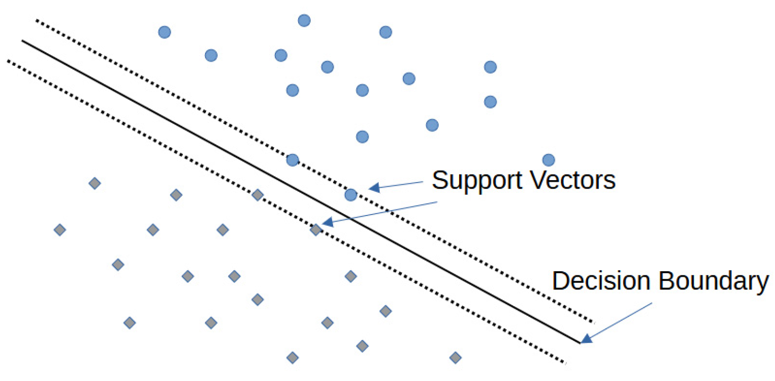
Figure 1. Higher-dimensional feature space via SVM, where a linear hyperplane can be identified to separate the classes, which can be mapped to the original space as a non-linear boundary line.
Electronics 14 03415 g001
Figure 2. Random forest (RF) architecture, where n DTs each consider a unique subset of features, with their predictions combined into a single decision.
Electronics 14 03415 g002
Figure 3. Multilayer perceptron (MLP) architecture example, with one neuron in the output layer used for classification purposes.
Electronics 14 03415 g003
Figure 4. CNN architecture: convolution layers are denoted as C, pooling layers are denoted as P, and fully connected layers are denoted as F.
Electronics 14 03415 g004
Figure 5. Steps of the proposed facial emotion recognition (FER) approach using ensemble learning and EfficientNet-B0 model.
Electronics 14 03415 g005
Figure 6. The confusion matrix for the multiclass classification experiment.
Electronics 14 03415 g006
Figure 7. Accuracy results as bar charts for binary classifiers of facial emotions.
Electronics 14 03415 g007
Figure 8. F1-score results as bar charts for all binary classifiers.
Electronics 14 03415 g008
Figure 9. The confusion matrix for the meta-classifier in the second experiment.
Electronics 14 03415 g009
Table 1. Average accuracies (%) for subject-independent and cross-database evaluations.
DatasetSubject-IndependentCross-Database
Multi-PIE94.745.7
MMI77.655.6
DISFA55.037.7
FERA76.739.4
SFEW47.739.8
CK+93.264.2
FER201366.434.0
Table 2. Relevant previous works on facial emotion recognition (FER).
AuthorsDatasetsArchitectureRecognition Accuracy
Liliana, Dewi Yanti [2]CK+ [2]CNN92.81% (two sets: training and test)
Mollahosseini et al. [3]Multi-PIE [53], MMI [54], DISFA [55], FERA [57], SFEW [58], CK+ [56], FER2013 [59]CNN94.7%, 77.6%, 55.0%, 76.7%, 47.7%, 93.2%, and 66.4%
Paweł et al. [4]KDEF [61]3-NN classifier and MLP neural network classifier95.5% for 3-NN classifier (two sets: training and test) and 75.9% for MLP classifier (three sets: training, validation, and test)
Mehendale [5]Caltech faces, CMU, and NIST [5]CNN96% (two sets: training and test)
Agrawal and Mittal [6]FER2013 [6]CNN65%
T.U. Ahmed et al. [7]CK and CK+ [56], FER2013 [63], MUG [64], KDEF and AKDEF [65], KinFaceW-I and -II [66]CNN96.24% validation accuracy
Kusuma Negara et al. [8]FER2013 [8]VGG-1669.40%
Rajesh Singh et al. [9]RAF-DB [69], FER2013 [9], and Cohn–Kanade [56]EfficientNet-B081.68% for RAF-DB
71.02% for FER2013
Cross-data on RAF-DB and CK+: 78.59%
Cross-data on RAF-DB and on FER2013: 56.10%
Rit Lawpanom et al. [10]FER2013 [10]HoE-CNNAchieved accuracy of 75.51%
Milind Talele et al. [11]FER2013 [11]Custom CNN and ResNet-5074% for custom CNN and 85.75% for ResNet-50 model
Sun et al. [12]RAF-DB [71], AffectNet [72], and FER2013 [12]AR-TE-CATFFNet89.50%, 65.66%, and 74.84%
Wasi [13]AffWild2 [73], RAF-DB [71], JAFFE [74], FERG-DB [75], and FER+ [76]W-BCSA-Vit and reliability balancing72.48%, 92.47%, 96.67%, 93.09%, and 98.18%
Table 3. Data splitting for experiments.
Experiment No.Experiment TypeTraining SplitValidation SplitTest Split
1Multiclass Classification70%15%15%
2Eight Binary Classifiers70%15%15%
Meta-Classifier70%15%15%
Table 4. Model configuration parameters.
ParameterMulticlass ModelBinary Model
Input Shape(224, 224, 3)(224, 224, 3)
Include TopFalseFalse
WeightsImageNetImageNet
Global Average PoolingAppliedApplied
Dropout Rate (1st)0.50.5
Output Dense Units81
Activation Function (Output)SoftMaxSigmoid
Intermediate Dense Layer16 neurons, ReLU16 neurons, ReLU
Batch NormalizationAppliedApplied
Dropout Rate (2nd)0.50.5
Table 5. The final class distributions for the binary classifiers.
Binary ClassifierPositive ClassNegative Class
Happy83468346
Sad96079607
Anger92489248
Fear99949994
Surprise96609660
Neutral10,03410,034
Disgust10,21210,212
Contempt10,70110,701
Table 6. Accuracy results for binary classifiers of facial emotions.
Binary ClassifierTraining AccuracyValidation AccuracyTesting Accuracy
1Happy99.8699.1298.68
2Sad99.9999.9099.61
3Anger99.9999.5099.74
4Fear99.9799.8399.69
5Surprise99.9999.6299.41
6Neutral99.9999.8399.90
7Disgust99.9999.9799.96
8Contempt10010099.90
Table 7. The F1-score results for all binary classifiers.
Binary ClassifierPrecisionRecallF1-Score
1Happy97.7999.4398.60
2Sad99.2199.9299.57
3Anger99.5710099.78
4Fear99.3210099.65
5Surprise98.8210099.40
6Neutral99.6610099.83
7Disgust99.9310099.96
8Contempt99.9310099.96
Disclaimer/Publisher’s Note: The statements, opinions and data contained in all publications are solely those of the individual author(s) and contributor(s) and not of MDPI and/or the editor(s). MDPI and/or the editor(s) disclaim responsibility for any injury to people or property resulting from any ideas, methods, instructions or products referred to in the content.