Wavelet-Based Denoising Strategies for Non-Stationary Signals in Electrical Power Systems: An Optimization Perspective

Abstract

Effective noise elimination is essential for ensuring data reliability in high-accuracy measurement systems. However, selecting the optimal denoising strategy for diverse and non-stationary signal types remains a major challenge. This study presents a wavelet-based denoising optimization framework that systematically identifies and applies the most suitable noise reduction model for each signal segment. By evaluating multiple wavelet types and thresholding strategies, the proposed method enables adaptive and automated selection tailored to the specific characteristics of each signal. The framework was validated using synthetic, open-access, and experimentally acquired signals in both reference-based and reference-free scenarios. Extensive testing covered signals from power quality disturbance (PQD) events, electrocardiogram (ECG) data, and electroencephalogram (EEG) recordings, all of which represent critical applications where signal integrity under noise is essential. The method achieved optimal model selection in 22.15 s (across 4558 iterations) on a standard PC, with an average denoising time of 4.86 ms per signal window. These results highlight its potential for real-time and embedded applications, including smart grid monitoring systems, wearable health devices, and automated biomedical diagnostic platforms, where adaptive, fast, and reliable denoising is vital. The framework’s versatility makes it highly relevant for deployment in smart grid monitoring systems and intelligent energy infrastructures requiring robust signal conditioning.

1. Introduction

It is a proven fact that noise is accountable for introducing irrelevant non-stationary signals, thereby degrading the quality of data analysis. Noise reduction is a critical component of signal processing. Signal quality has a direct impact on the precision and trustworthiness of analyses in all areas of engineering, specifically in high-stakes disciplines, such as structural health monitoring, biomedical signal processing, and fault diagnosis. Machine learning and deep learning (DL) techniques have recently demonstrated great potential for noise cancelation by effectively handling complex noise features and improving signal quality. Among the techniques reported in the literature, the discrete wavelet transform (DWT) is the leading method for noise cancelation. The literature has highlighted the potential of the transform method to maximize the denoising of signals and underlined the contribution of wavelets in noise cancelation [1]. Wavelet approaches have numerous applications in various fields, particularly biomedical signal denoising. For example, studies have presented effective wavelet-denoising algorithms and compared their capacities to provide precise noise elimination [2]. These contributions demonstrate the necessity of employing WT as a general denoising tool. Thorough comparisons of image-denoising algorithms exist, encompassing both heuristic optimization and dictionary learning approaches [3]. This research sheds light on the evolution of denoising methods, showing higher efficiency than other methods combined with WT. Moreover, research on group-sparse signal denoising methods has shown a novel framework for noise reduction with greater efficiency in the treatment of complicated signals [4].

Noise suppression in non-stationary signals has emerged as a critical task in power systems, biomedical monitoring, and industrial control, where signal integrity directly influences decision-making and system reliability. Traditional denoising techniques often fall short in capturing the transient, multiscale, and context-specific characteristics of such signals [5,6,7]. Recent literature has seen a shift toward hybrid and data-driven strategies, where wavelet-based approaches are coupled with empirical methods, optimization algorithms, and deep learning models to improve noise reduction performance across various domains [8,9,10,11,12,13]. Empirical wavelet transforms (EWT) [8], variational mode decomposition (VMD) [9], and adaptive multiscale techniques [10,14] have shown notable promise in extracting useful signal components from noisy measurements.

EWT has proven effective in handling non-stationary signals through adaptive frequency band partitioning, making it highly applicable to Electrocardiography (ECG) and power disturbance signals. Notably, recent work has introduced entropy-guided segment tracking to improve EWT-based ECG denoising performance [15,16,17]. However, EWT methods still face challenges in boundary selection and noise folding during empirical segmentation. VMD offers superior mode separation and has demonstrated effectiveness in power signal analysis [18], yet its performance relies heavily on predefined decomposition parameters, which limit its flexibility. Deep learning approaches, including autoencoders and attention-based models, exhibit state-of-the-art performances in noise suppression across biomedical domains, but they require substantial training data and often lack transparency in how decisions are made [13,19].

In biomedical domains, convolutional neural networks (CNNs) and transformer-based architectures have enhanced denoising performance, especially for ECG and Electroencephalography (EEG) signals under dynamic noise environments [20,21]. Similarly, in power quality disturbance (PQD) analysis, adaptive wavelet thresholding [10], dual-domain filtering [22], and deep residual learning [12] have enabled real-time implementation with improved accuracy. Moreover, entropy-guided filtering [8,23], noise-aware generative learning [24], and cross-domain joint entropy wavelets [25] are increasingly being adopted for robust feature preservation during denoising. Still, a critical bottleneck remains: the automated and optimized selection of the best-fit denoising model based on the type and dynamics of the incoming signal. The importance of denoising has also been demonstrated in practical implementations of signal-based damage detection frameworks, where reliable signal clarity significantly improves machine learning performance, particularly under limited data conditions [26].

In the past several years, there have been important advances in wavelet-based denoising techniques, in which the design of new optimization methods has been crucial for progress in this area. Among the key advances has been the idea of artifact-free wavelet denoising software, which has been effective in inhibiting artifacts in the denoising process and maintaining the integrity of the signal structure [27]. These approaches have utilized nonconvex sparse regularization, a procedure that is useful in this application.

An optimization method based on the Hilbert–Huang transform for signal denoising has been demonstrated to be effective for noise removal [28], indicating the advancement and variety of denoising methods. In the field of biomedical signal processing, extensive research on noise removal methods for ECG signals has been conducted to evaluate the performance of WT, empirical mode decomposition (EMD), and other techniques to establish best practices for noise reduction [29].

The field has also witnessed considerable development with the arrival of DL-based methodologies, including effective empirical mode analysis [30] and deep factor analysis-based methods [31], which have revolutionized ECG signal denoising. These are instrumental in biomedical signal analysis and interpretation. Research investigating the effectiveness of noise removal in phonocardiography signals using wavelet-based decomposition has yielded significant findings [32]. In addition, studies on the denoising of surface electromyography signals have demonstrated improved performance using ensemble EMD with optimized wavelet thresholds [33]. A comprehensive evaluation of wavelet-based denoising methods for neural signal processing indicates the best practices in this field [34]. These reviews indicate that it is necessary to combine other advanced methods with the WT. Structural health monitoring has been promoted by the application of advanced denoising techniques like residual CNNs, which have achieved remarkable vibration signal denoising with the capacity to reduce noise and sustain important features [35].

Noise reduction techniques have universal applications in a variety of disciplines, and technology has further enhanced these techniques. For example, new approaches have been suggested to mitigate noise and improve the detection of defects in natural gas pipelines [36], while denoising algorithms for transient electromagnetic signals have been developed to enhance reliability [37]. Likewise, recent advances in the denoising of underwater acoustic signals have prompted the development of robust algorithms that can withstand various types of noise [38]. An effective noise-removal system has also been developed to improve the reliability of ECG signals [39], and a hybrid method has been applied to EEG signal denoising [40]. In the field of atmospheric data analysis, recurrent NNs have proven helpful in removing atmospheric noise from interferometric synthetic aperture radar time series, despite dealing with missing data, thereby depicting the versatility of DL when it comes to environmental noise control [41].

Various denoising techniques have been explored to enhance signal fidelity for biomedical applications, such as ECG signal processing. A comprehensive review outlined various noise-removal techniques for ECG signals, emphasizing the ongoing improvement and evaluation of effective approaches in this field [42]. Specific techniques, such as conditional Generative Adversarial Networks (GANs), have been employed to denoise ECG signals by leveraging generative modeling to enhance signal clarity [43]. In addition, the application of weighted stationary wavelet total variation approaches has been effective in the processing of nonstationary noise patterns in ECG denoising [44]. Furthermore, the application of variational mode decomposition algorithms has been shown to improve denoising performance by applying adaptive decomposition strategies, which in turn improve signal accuracy [45]. GAN-based approaches are employed in image denoising, where optimization algorithms integrated with GANs effectively reduce image noise, thereby showing the cross-domain applicability of the advanced denoising techniques [46].

This study presents a denoising optimization method using different scenarios with various wavelet types for non-stationary PQD signals. Therefore, the most reliable signals can be obtained for different signal types without any additional requirements. As can be understood from these studies, advances in denoising methods in various applications improve signal quality and reliability. However, most studies have focused on a specific signal type. This causes incompatibility with the methods in the presence of non-stationary signals other than a specific signal type. Hence, a denoising method that is compatible with most signal types is required to simplify the process. Therefore, the methods in this study can be applied to all fields related to signal quality as well as denoising studies in biomedical signals. To address these gaps, the present study proposes a novel optimization-based framework that systematically identifies the optimal wavelet and denoising method for each signal segment. By integrating wavelet-domain decomposition, entropy features, and heuristic optimization, the proposed method delivers adaptive noise suppression across power, biomedical, and synthetic signals. The efficacy of the approach is validated on a diverse set of datasets, including open-access and experimental signals, highlighting its potential for scalable, real-time deployment in critical systems.

The main contributions of this study are as follows.

• This is the first study to consist of a detailed study not only of medical but also of experimental PQD signals, exploring a vast parameter space through 4558 iterations.
• The proposed methodology demonstrates robustness in reference-based and reference-free signal processing scenarios.
• The algorithm was rigorously tested over a wide noise range (1–50 dB) by validating it with synthetically generated signals as well as specific benchmark signals from the literature, demonstrating a reliable performance even in high-noise environments.
• Experimental evaluations using PQD signals further substantiated the effectiveness of the method, highlighting its potential for practical applications.

The structure of this study is as follows: First, details of the wavelet denoising method and power quality are provided. The evaluation metrics for the signal quality are then provided. Subsequently, the proposed denoising optimization method is presented. Subsequently, the proposed method is evaluated using different synthetic and experimental signal types under noisy-level scenarios, and the results are discussed in detail. Finally, the conclusions are presented.

2. Materials and Method

Signals in the field may contain noise, which can lead to errors in measuring and assessing signals for critical events. Another problem is that there are no techniques compatible with all non-stationary signal types, such as fundamental, biomedical, and power system signals. Therefore, noise must be minimized using a technique that provides denoising to most signals as much as possible. Details of this process are provided below.

2.1. Wavelet-Based Denoising Techniques for Signal Processing

Wavelet denoising has become a critical approach in diverse signal processing applications where preserving signal integrity while reducing noise is essential. The selection of an optimal wavelet type, such as orthogonal or biorthogonal, is fundamental because it influences both the localization properties and reconstruction fidelity. The commonly used and orthogonal wavelet families, such as Daubechies (db), Symlets (sym), and Haar (haar) are distinguished from biorthogonal families like Biorthogonal Spline (bior), with each offering unique advantages based on signal characteristics and desired outcome [35,41].

The mathematical model for a noisy signal is represented as follows:

$$x_{noisy}\left(t\right)=x\left(t\right)+\sigma n\left(t\right)$$

(1)

where $x_{noisy}\left(t\right)$ is the observed signal, $x\left(t\right)$ is the original (noise-free) signal, σ represents the noise level, and $n\left(t\right)$ is assumed to be a Gaussian white noise with a mean of zero and unit variance. The objective of denoising is to recover $x\left(t\right)$ by attenuating noise $n\left(t\right)$ as effectively as possible [42].

The denoising process follows a three-stage pipeline as can be seen from Figure 1:

1.

Transform: $X=W\left(x_{noisy}\left(t\right)\right)$ where $W$ denotes the DWT.

2.

Thresholding: $\tilde{X}=T\left(\mathrm{X}\right)$, where $T(\cdot )$ is a thresholding operator (e.g., soft, or hard).

3.

Reconstruction: $\widehat{x}\left(t\right)=W^{-1}\left(\tilde{X}\right)$, yielding the denoised estimate.

Figure 1. Three-stage pipeline of denoising.

This framework abstracts away language-specific implementation differences and ensures that all methods align with a shared mathematical structure.

Various thresholding methods have been employed to adjust wavelet coefficients and minimize noise, each of which is suitable for different data structures. For instance, Bayes leverages an empirical Bayesian thresholding rule, assuming that measurements have prior independent distributions, as part of a mixture model. This is particularly advantageous in applications with larger datasets, where the posterior median can be used to minimize risk [47]. By adaptively optimizing block sizes, BlockJS enhances flexibility at both local and global levels, making it extremely well suited to intricate signal structures [43]. False Discovery Rate (FDR) improves threshold values by managing the rate of false alarms, ultimately yielding an asymptotic minimax estimator that is extremely efficient for sparse data applications [48]. Thresholds are set to reduce the maximum root mean square error (RMSE) to guarantee a conservative denoising procedure in the minimax method [49]. Stein’s Unbiased Risk Estimate (SURE) minimizes the risk function by providing an optimal threshold to minimize the MSE using an unbiased risk estimate [50,51]. Universal Threshold (UT) employs a universal threshold of √(2ln(L)), where L is the signal length. Universal thresholding works extremely well for large datasets and is extensively used in image and biomedical signal processing [52,53]. To implement the proposed algorithm, approximately 1000 lines of code have been prepared and run.

2.2. Basic Denoising Procedure

The denoising process generally consists of three steps: The signal is split into wavelet coefficients at various levels of $Max\_Level$, with segregation between noise and the original signal enabled in the decomposition step. A suitable threshold, usually a soft thresholding approach, is applied at every scale to alter the detail coefficients and eliminate noise in the detail coefficient thresholding. The reconstructed clean signal is obtained by adding the original approximation to the modified detail coefficients in the last step, reconstruction.

By appropriately selecting the thresholding rule, such as soft thresholding for SURE and Universal Thresholding or hard thresholding for FDR, wavelet denoising procedures offer adaptability to different signal types [2,4]. Noise variance estimation, which is a major determinant of denoising performance, can be level-independent (derived from the highest-resolution coefficients) or level-dependent (performed at each resolution level), thereby affecting the sensitivity to local variations in noise.

2.3. Denoising Evaluation Metrics

These denoising methods, measured using evaluation metrics, have demonstrated considerable success in recent studies for applications such as ECG signal noise reduction in [27,28] image denoising via GANs [29], and structural health monitoring using a residual CNN [30]. For example, the integration of recurrent neural networks in denoising atmospheric noise from interferometric synthetic aperture radar time series has shown promise in overcoming the challenges posed by missing values in time series data, thus enhancing the denoising precision for complex datasets [32]. All these methods use evaluation metrics such as RMSE and signal-to-noise ratio (SNR).

As given in [29], the RMSE and ${SNR}_{improvement}$ were computed to evaluate the performance of the denoising method using Equations (2)–(5).

$$RMSE=\sqrt{{\displaystyle \frac{1}{N}}{\sum }_{i=1}^N{[x_{denoised}\left(i\right)-x\left(i\right)]}^2}$$

(2)

$${SNR}_{improvement}={SNR}_{denoised}-{SNR}_{noisy}$$

(3)

$${SNR}_{noisy}=10\times {log}_{10}({\displaystyle \frac{\sum _{i=1}^N{\left[x\left(i\right)\right]}^2}{\sum _{i=1}^N{[x_{noisy}\left(i\right)-x\left(i\right)]}^2}})$$

(4)

$${SNR}_{denoised}=10\times {log}_{10}({\displaystyle \frac{\sum _{i=1}^N{\left[x\left(i\right)\right]}^2}{\sum _{i=1}^N{[x_{denoised}\left(i\right)-x\left(i\right)]}^2}})$$

(5)

Moreover, another performance metric was applied to the denoised signal using Equation (6) [45].

$${Corr}_{coef}={\displaystyle \frac{\sum _{i=1}^N\left(x\left(i\right)-\overline{x}\right)(x_{denoised}\left(i\right)-\overline{x_{denoised}})}{\sqrt{\sum _{i=1}^N{\left(x\left(i\right)-\overline{x}\right)}^2{(x_{denoised}\left(i\right)-\overline{x_{denoised}})}^2}}}$$

(6)

These formulations help distinguish actual performance gain over baseline noisy data. Based on Equation (3), SNR_imp (%), MSE_imp (%), RMSE_imp (%), and Corrcoef_imp (%) are given as the following Equations (7)–(10), respectively. These formulations help distinguish actual performance gain over baseline noisy data.

$${SNR}_{imp}(\%)={\displaystyle \frac{{SNR}_{denoised}-{SNR}_{noisy}}{{SNR}_{noisy}}}$$

(7)

$${MSE}_{imp}(\%)={\displaystyle \frac{{MSE}_{denoised}-{MSE}_{noisy}}{{MSE}_{noisy}}}$$

(8)

$${RMSE}_{imp}(\%)={\displaystyle \frac{{RMSE}_{denoised}-R{MSE}_{noisy}}{{RMSE}_{noisy}}}$$

(9)

$${Corrcoef}_{imp}(\%)={\displaystyle \frac{{Corrcoef}_{denoised}-{Corrcoef}_{noisy}}{{Corrcoef}_{noisy}}}$$

(10)

To better interpret the denoising performance, we calculate four improvement indicators. ${SNR}_{imp}$ (%) gives the percentage result for SNR improvement. ${MSE}_{imp}$ (%) quantifies the relative reduction in squared error energy. ${RMSE}_{imp}$ (%) offers a perceptual error measure with the same physical units as the original signal. Correlation Coefficient Improvement ${Corrcoef}_{imp}$ (%) highlights the degree to which signal morphology is recovered post-denoising. This is particularly valuable in biomedical signals such as ECG or EEG, where waveform fidelity is critical.

2.4. Denoising Evaluation Test Signals

The method proposed in this paper was tested with different signal types, such as a basic signal and a biomedical or power quality signal, as given in Table 1, under different noise SNR ranges.

Table 1. Labels of test signals.

Test Signal	Label	Test Signal	Label
$v_1\left(t\right)$ signal in Table 2 for Equation (1)	L1	Equation (15) signal in [40]	L4
Equation (11) signal in [36]	L2	Experimental PQD signals in Table 2	L5
Arrhythmia data in [54]	L3

First, the basic signal form of the noisy signal in (1) was evaluated, and the results were detailed. This evaluation was true for all the signal types.

The other signal dataset is made up of 50, 200, and 250 Hz components in [36], as in Equation (11).

$$x\left(t\right)=4\sin \left(100\pi t\right)+0.2\sin \left(400\pi t\right)+0.2\cos \left(500\pi t\right)$$

(11)

Another signal dataset based on the Arrhythmia data in [54], an ECG signal, was considered.

The final test signals, comprising components with different frequencies [40], were considered. $x_1\left(t\right)$ in Equation (12) and $x_2\left(t\right)$ in Equation (13), and $x_3\left(t\right)$ in Equation (14), represent amplitude-modulated, harmonic, and exponentially decaying signals, respectively. $x\left(t\right)$ in Equation (15), which is an EEG signal, consists of:

$$x_1\left(t\right)=\left(1+m\times \mathit{sin}\left(2\pi 4t\right)\right)\times (0.5\times \mathit{sin}\left(2\pi 18t\right))$$

(12)

$$x_2\left(t\right)=\mathit{sin}\left(2\pi 30t\right)+2\times \mathit{sin}\left(2\pi 60t\right)$$

(13)

$$x_3\left(t\right)=\mathit{sin}\left(2\pi 60t\right)\times e^{-0.5t}$$

(14)

$${x\left(t\right)=x_1\left(t\right)+x_2\left(t\right)+x}_3\left(t\right)$$

(15)

All the test signals with noise n(t) in Equation (16) are evaluated under different noise ranges for n(t) and the evaluation metrics.

$$v_{test}\left(t\right)=x\left(t\right)+n\left(t\right)$$

(16)

The experimental signals, whose equations are listed in Table 2, were then analyzed. These signals have a natural grid noise, $n_{grid}$, as shown in Equation (17). Hence, they did not require additional noise evaluation. These were obtained from a setup consisting of an adjustable power source and oscilloscope, like in Figure 2:

Table 2. Equations for experimental PQD data.

$$\begin{gathered} \mathbf{Case} \\ \left(\mathit{k}\right) \end{gathered}$$	Definition	Model Equation	Noisy Model	Parameter
1	Pure	$v_1\left(t\right)=\mathrm{s}\mathrm{i}\mathrm{n}\left(2\pi f_{0}t\right)$	$v\left(t\right)=v_k\left(t\right)+n_{grid}\left(t\right)$	${49.5\le f}_0\le 50 \mathrm{Hz}$
2	Sag	$v_2\left(t\right)=[1-{\alpha }_{sag}(u\left(t-t_1\right)-u\left(t-t_2\right)\left)\right]v_1\left(t\right)$		$0.1\le$ ${\alpha }_{sag}\le 0.9$ $T_0\le t_2-t_1\le 9T_0$ $T_0=1/f_0$ $u:\mathrm{u}\mathrm{n}\mathrm{i}\mathrm{t}\hspace{0.17em}\mathrm{s}\mathrm{t}\mathrm{e}\mathrm{p}\hspace{0.17em}\mathrm{f}\mathrm{u}\mathrm{n}\mathrm{c}\mathrm{t}\mathrm{i}\mathrm{o}\mathrm{n}$
3	Swell	$v_3\left(t\right)=[1+{\alpha }_{swell}(u\left(t-t_1\right)-u\left(t-t_2\right)\left)\right]v_1\left(t\right)$		$0.1\le$ ${\alpha }_{swell}\le 0.8$ $T_0\le t_2-t_1\le 9T_0$
4	Flicker	$v_4\left(t\right)=[1+{\alpha }_{flicker}\mathrm{s}\mathrm{i}\mathrm{n}(2\pi f_{flicker}t\left)\right]v_1\left(t\right)$		$0.05\le$ ${\alpha }_{flicker}\le 0.279$ $1 \mathrm{Hz}\le f_{flicker}\le 25 \mathrm{Hz}$
5	Harmonics	$v_5\left(t\right)=v_1\left(t\right)+{\alpha }_3\mathit{sin}\left(2\pi {3f}_{0}t\right)+{\alpha }_5\mathit{sin}\left(2\pi {5f}_{0}t\right)+{\alpha }_7\mathit{sin}\left(2\pi {7f}_{0}t\right)$		$0.05\le$ ${\alpha }_3, {\alpha }_5,{\alpha }_7\le 0.5$
6	Spikes	$$\begin{gathered} v_6\left(t\right)=v_1\left(t\right)+sign\left(v_1\left(t\right)\right)\left\{{\displaystyle \sum _{n=0}^9}{\alpha }_{spikes}⟨\left[u\left(t-{(t}_3+0.02n)\right) \\ \hspace{1em}\hspace{1em}\hspace{1em}\hspace{1em}\hspace{1em}\hspace{1em}\hspace{1em}-u\left(t-{(t}_4+0.02n)\right)\right] \\ \hspace{1em}\hspace{1em}\hspace{1em}\hspace{1em}\hspace{1em}\hspace{1em}\hspace{1em}-\left[u\left(t-{(t}_5+0.02n)\right)-u\left(t-{(t}_6+0.02n)\right)\right]⟩\right\} \end{gathered}$$		$0.2\le$ ${\alpha }_{spike}\le 0.4$ $0\le t_3, t_4\le 0.5T_0$ ${0.01T}_0\le t_4-t_3\le 0.05T_0$ $0.5T_0\le t_5, t_6\le T_0$ ${0.01T}_0\le t_6-t_5\le 0.05T_0$
7	Sag and Harmonics	$v_7\left(t\right)=[1-{\alpha }_{sag}(u\left(t-t_1\right)-u\left(t-t_2\right)\left)\right]v_5\left(t\right)$		$0.1\le$ ${\alpha }_{sag}\le 0.9$ $T_0\le t_2-t_1\le 9T_0$ $T_0=1/f_0$

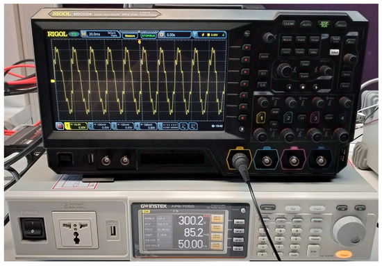
Figure 2. Experimental setup for PQD data acquisition.

Adjustable AC Power Supply: A programmable AC power supply (APS 7050, 500 W) manufactured by GW Instek (Good Will Instrument Co., Ltd., New Taipei City, Taiwan) was used.

Oscilloscope: A mixed-signal oscilloscope (MSO 5204) manufactured by Rigol Technologies, Inc. (Suzhou, China) was utilized.

All measurements were conducted using the specified equipment, and calibration was verified prior to testing.

It provides seven different types of noisy PQD signals.

$$v\left(t\right)=v_k\left(t\right)+n_{grid}\left(t\right)$$

(17)

3. Proposed Denoising Optimization Method

The proposed method is defined hierarchically as follows.

3.1. Defining Variables and Acquisition of Denoised Signals

All the variables are first defined at the beginning of the algorithm, as shown in Figure 3. Table 3 provides the definitions of the variables in detail. Then, the “glp” for the loop is launched to acquire the denoised signals. Each offer starts with a new step for the selection of wavelet types, from “sym” to “coif”. Details of this new step are presented in the next section.

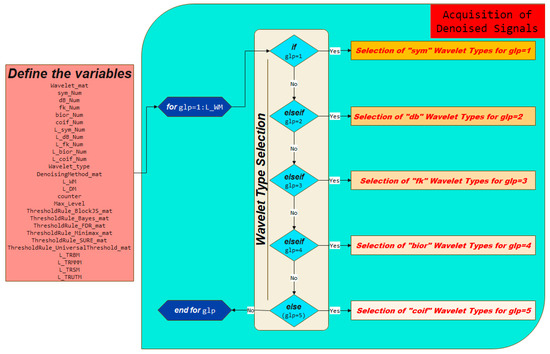
Figure 3. Flowchart for proposed method.

Table 3. Definitions of the variables.

Variable	Definition	Value
Wavelet_mat	Wavelet Types	[“sym”, ”db”, ”fk”, ”bior”, ”coif”]
sym_Num	Number of Sym Wavelet	[2:1:8]
db_Num	Number of db Wavelet	[1:1:10]
fk_Num	Number of fk Wavelet	[4, 6, 8, 14, 18, 22]
bior_Num	Number of bior Wavelet	[1.1, 1.3, 1.5, 2.2, 2.4, 2.6, 2.8, 3.1, 3.3, 3.5, 3.7, 3.9, 4.4, 5.5, 6.8]
coif_Num	Number of coif Wavelet	[1:1:5]
DenoisingMethod_mat	Denoising Method Types	[“BlockJS”, ”Bayes”, ”FDR”, ”Minimax”, ”SURE”, ”UniversalThreshold”]
wavelet_type	Wavelet Type	merge(Wavelet_mat(i),num2str(sym_Num(symlp)))
Max_Level	Maximum Level of Denoising Method	[7, 9]
L_DM	Length of DenoisingMethod_mat	6
L_WM	Length of Wavelet_mat	5
ThresholdRule_BlockJS_mat	ThresholdRules of BlockJS	[“James-Stein”]
ThresholdRule_Bayes_mat	ThresholdRules of Bayes	[“Median”, ”Mean”, ”Soft”, ”Hard”]
ThresholdRule_FDR_mat	ThresholdRules of FDR	[“Hard”]
ThresholdRule_Minimax_mat	ThresholdRules of Minimax	[“Soft”, ”Hard”]
ThresholdRule_SURE_mat	ThresholdRules of SURE	[“Soft”, ”Hard”]
ThresholdRule_UniversalThreshold_mat	ThresholdRules of UniversalThreshold	[“Soft”, ”Hard”]
L_TRBM	Length of ThresholdRule_Bayes_mat	4
L_TRMMM	Length of ThresholdRule_Minimax_mat	2
L_TRSM	Length of ThresholdRule_SURE_mat	2
L_TRUTM	Length of ThresholdRule_UniversalThreshold_mat	2

3.2. Selection of Wavelet Types

Through the launching of the “glp” loop, wavelet types can be selected. For glp = 1, the “sym” wavelet type is selected, as shown in Figure 4. Subsequently, another loop can be initiated for the degree of this wavelet in the range of 2–8. Another subloop with “lp” is run to define the Denoising Method Selection in detail. Details of this loop are provided in the next section. For the case of glp = 2, the “dblp” wavelet was selected, and another loop was run in the range of 1–10. The rest of the process was the same as that for the “symlp” loop. This process is repeated for the other wavelet types for different values of “glp” in the loop correspondence to “fklp”, “biorlp”, and “coiflp”, respectively.

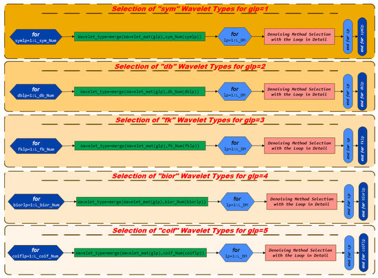
Figure 4. Flowchart of selection of wavelet types for specific parameter subblocks.

3.3. Denoising Model Selection with the Loop in Detail and Saving

This section provides a detailed explanation of the “Denoising Model Selection with the Loop in Detail” layer, as employed in the “Selection of Wavelet Types” phase, concerning the flowchart presented in Figure 5.

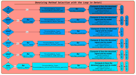
Figure 5. Flowchart of denoising method selection subblock.

In this subsection of the proposed algorithm, one of the denoising methods, “BlockJS”, “Bayes”, “FDR”, “Minimax”, “SURE”, or “UniversalThreshold” is selected. When only a single thresholding technique is applied, as in the case of “lp = 1”, the “James-Stein” method is executed, and the inner “k” loops are directly initiated. In scenarios where different thresholding techniques are considered, like the “Bp” loop, as seen in “lp = 2”, encompassing thresholding strategies such as “Median”, “Mean”, “Soft”, and “Hard” are used to refine the denoising process.

Through the iterative execution of the “k” loops, the algorithm applies the designated denoising method up to the predefined maximum level. The cleaned signal and its corresponding model are stored systematically in each iteration for subsequent evaluation. This structured approach ensures a comprehensive search for the most effective denoising model while maintaining computational efficiency. The procedural framework remained consistent across different selection scenarios with variations in the specifics of the denoising method employed.

The entire architecture has been designed to support modularity, scalability, and adaptability to evolving signal processing methods. As outlined in both the parameter table and flowchart (Figure 3, Figure 4 and Figure 5), wavelet type selection is handled in a loop-based structure where each wavelet family, defined in the Wavelet_mat array, is iteratively processed using the associated subtypes (e.g., sym_Num, db_Num, fk_Num, etc.).

Similarly, the denoising method selection logic is parametrically constructed through the DenoisingMethod_mat variable, where each method is linked to its corresponding thresholding rules via structured matrices such as ThresholdRule_Bayes_mat, ThresholdRule_SURE_mat. The optimization engine then evaluates all combinations of (wavelet type × decomposition level × denoising method × thresholding rule), based on a pre-defined performance metric like SNR, or MSE. If a new wavelet family (for instance “new_wlt”) is to be introduced, the system can incorporate it by simply:

• Appending the new name to the Wavelet_mat array (e.g., Wavelet_mat = [“sym”, …, “new_wlt”]),
• Defining its subtype range in a corresponding vector (like new_wlt_Num = [1,2,3]),
• The glp loop’s conditionals are extended to handle the new branch.
• Similarly, for new denoising methods, such as threshold-free neural filters or transformer-based denoisers, the following changes would suffice:
• Add the new method to DenoisingMethod_mat,
• Define a new threshold rule matrix (if applicable), such as ThresholdRule_DL_mat = [“Soft”, “Hard”, “Learned”],
• Include a maximum decomposition level entry in Max_Level,
• Extend the corresponding loop bounds or switch-case logic if necessary.

Importantly, no changes to the core algorithmic logic or the optimization structure would be needed, as the framework dynamically parses the parameter arrays. The use of indexing (glp, or new_wlt) and matrix-based rule assignment ensures that any number of wavelet families, or methods, can be handled at runtime without any structural re-coding.

Thus, the system’s forward compatibility with emerging denoising technologies is preserved by design. This ensures that the framework is not only robust for current state-of-the-art methods but also readily extensible for future research directions.

3.4. Evaluation of All the Saved Denoised Signals

As illustrated in Figure 6, this layer systematically evaluates the denoised datasets and models obtained upon completion of the iterative process. Various quantitative metrics were used to obtain the most accurate results. The availability of the original reference signal was a critical determinant of this evaluation. In cases where a reference signal was unavailable, all 4558 generated combinations were assessed based on their SNRs to select the time-series signal exhibiting the lowest residual noise. Conversely, when a reference signal was available, the analysis included MSE, RMSE, and Corr metrics across all combinations. The optimal denoised signal was determined based on the RMSE, ensuring consistency among all evaluation criteria.

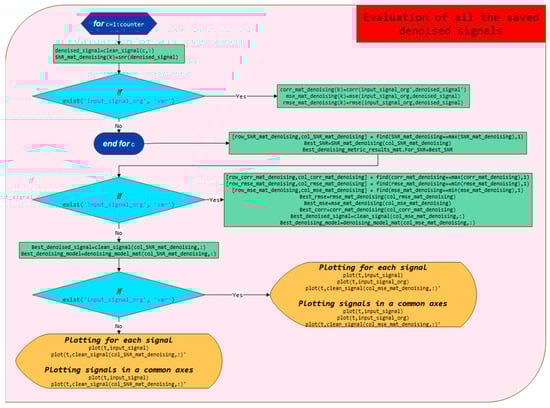
Figure 6. Flowchart of denoised signal evaluation.

For comparative visualization, a three-layered signal representation was generated if a reference signal was present. Otherwise, the visualization consisted of a dual-layer representation that depicts noisy and denoised signals in overlaid and separate formats. The entire evaluation process is encapsulated within a single function, with the parameter specifications detailed in Table 4. The corresponding denoised parameter cloud is illustrated in Figure 7. The exhaustive search across 4558 combinations was completed within 22.15 s, with an average denoising execution time of 4.86 ms. These results confirm the suitability of the algorithm for real-time signal-processing applications.

Table 4. Research parameter space.

Parameter	Count	Parameter	Count	Parameter	Count	Parameter	Count	Parameter	Count	Parameter	Count
1	516	FDR	387	bior1.5	106	bior5.5	106	db4	106	fk8	106
2	516	Hard	1935	bior2.2	106	bior6.8	106	db5	106	sym2	106
3	516	James-Stein	301	bior2.4	106	coif1	106	db6	106	sym3	106
4	516	Mean	387	bior2.6	106	coif2	106	db7	106	sym4	106
5	516	Median	387	bior2.8	106	coif3	106	db8	106	sym5	106
6	516	Minimax	774	bior3.1	106	coif4	106	db9	106	sym6	106
7	516	SURE	774	bior3.3	106	coif5	106	fk14	106	sym7	106
8	473	Soft	1548	bior3.5	106	db1	106	fk18	106	sym8	106
9	473	UniversalThreshold	774	bior3.7	106	db10	106	fk22	106
Bayes	1935	bior1.1	106	bior3.9	106	db2	106	fk4	106
BlockJS	301	bior1.3	106	bior4.4	106	db3	106	fk6	106

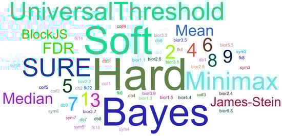
Figure 7. Denoised parameter cloud.

While the proposed adaptive wavelet-based denoising method is based on established techniques, the novelty of the present study lies in its comprehensive optimization strategy that simultaneously explores multiple wavelet families, decomposition levels, denoising methods, and thresholding rules. This framework enables signal-specific tuning, which enhances performance across diverse domains and noise profiles.

4. Results and Discussion

The proposed signal was applied to different signal types, from pure to experimental. The details are as follows:

4.1. Results for the Pure Signal, $L1,$ in the Case of the Original Signal

A pure sinusoidal signal, $v_1\left(t\right)$ with a 100 V amplitude, 50 Hz frequency, and 10 dB SNR noise, is shown in Figure 8. As shown in the figure, the noisy input signal is denoised as much as possible, although it is highly noisy. As is illustrated in Figure 8d, the denoised signal is compatible with the original signal, with some small errors.

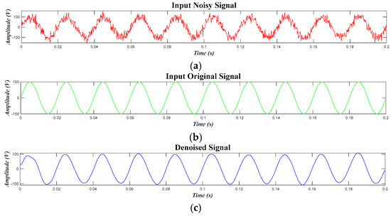
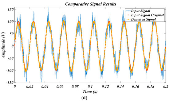
Figure 8. Comparative waveforms of L1 signals in the presence of the original signal: (a) noisy input signal, (b) original input signal, (c) denoised signal, (d) comparative signal results.

Another test of this signal was performed without the original signal. It can be understood from Figure 9c that the denoised signal can be estimated from a highly noisy signal. When the proposed method is compared with the help of this figure and Figure 8 for cases with the presence or absence of the original signal, it is observed that the first case is more compatible with the original signal. Therefore, the original signal option is used in the remainder of the study if the original signal is available.

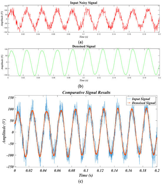
Figure 9. Comparative Waveforms of the signals in the absence of the original signal: (a) input noisy signal, (b) denoised signal, (c) comparative signal results.

4.2. Results of Test Signals

Since test signals yielded the most effective denoising performance under varying wavelet parameters across different SNR levels, the results and corresponding parameters within the range of 1–50 dB are presented and discussed in detail below. In particular, the inclusion of low SNR levels, starting from as low as 1 dB, is critical for demonstrating the algorithm’s ability to achieve substantial improvements under severe noise conditions.

4.2.1. Results for $L2$ for Different SNR Levels

Another signal that needs to be obtained is the $x\left(t\right)$ signal in Equation (11). Noise at different SNR levels was injected into this signal from 1 dB to 50 dB. As can be understood from Figure 10d, the denoised signal at 1 dB SNR is estimated from the highly noisy signal. However, it differs from the original signal because of its high noise level. Another waveform obtained from the same signal at 50 dB SNR, which is an almost noise-free environment, is shown in Figure 11. This is more compatible with the original signal.

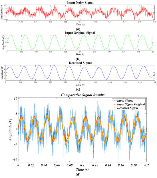
Figure 10. Comparative waveforms of L2 under SNR = 1 dB: (a) noisy input signal (b) original input signal, (c) denoised signal, (d) comparative signal results.

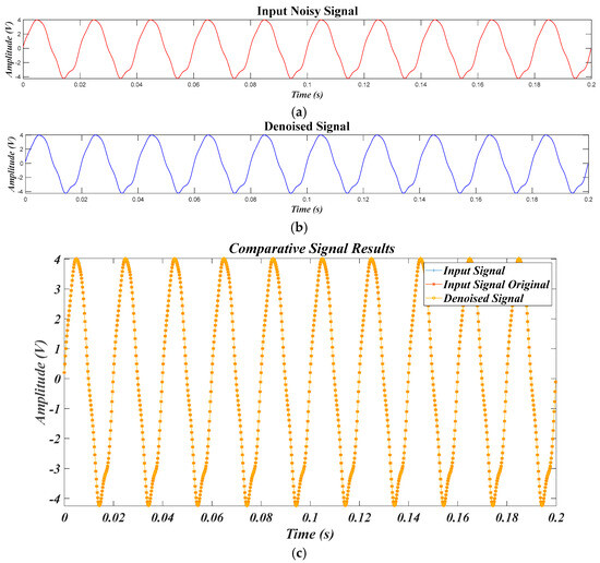
Figure 11. Comparative waveforms of L2 under SNR = 50 dB: (a) noisy input signal, (b) denoised signal, (c) comparative signal results.

These results provide insight into the performance of the proposed method, but not in detail. Therefore, Table 5 was prepared to show different performance metrics, such as SNR, MSE, RMSE, Corr, ${SNR}_{imp}$, ${RMSE}_{imp}$, ${MSE}_{imp}$, and ${Corr}_{imp}$ under different noise levels in the range of 1 dB to 50 dB. The ${SNR}_{denoised}$ results, which increase with the SNR level, bring about the recovery of ${SNR}_{imp}$. This is also true for Corr and ${Corr}_{imp}$, which converge to 1 as desired. Conversely, this table provides decremental MSE and RMSE results that approach zero. Hence, improvements, such as ${RMSE}_{imp}$ and ${MSE}_{imp},$ are preferable.

Table 5. Metric results for L2.

${\mathit{S}\mathit{N}\mathit{R}}_{\mathit{n}\mathit{o}\mathit{i}\mathit{s}\mathit{y}}$	${\mathit{S}\mathit{N}\mathit{R}}_{\mathit{d}\mathit{e}\mathit{n}\mathit{o}\mathit{i}\mathit{s}\mathit{e}\mathit{d}}$	${\mathit{S}\mathit{N}\mathit{R}}_{\mathit{i}\mathit{m}\mathit{p}}$ (%)	${\mathit{R}\mathit{M}\mathit{S}\mathit{E}}_{\mathit{n}\mathit{o}\mathit{i}\mathit{s}\mathit{y}}$	${\mathit{R}\mathit{M}\mathit{S}\mathit{E}}_{\mathit{d}\mathit{e}\mathit{n}\mathit{o}\mathit{i}\mathit{s}\mathit{e}\mathit{d}}$	${\mathit{R}\mathit{M}\mathit{S}\mathit{E}}_{\mathit{i}\mathit{m}\mathit{p}}$ (%)	${\mathit{M}\mathit{S}\mathit{E}}_{\mathit{n}\mathit{o}\mathit{i}\mathit{s}\mathit{y}}$	${\mathit{M}\mathit{S}\mathit{E}}_{\mathit{d}\mathit{e}\mathit{n}\mathit{o}\mathit{i}\mathit{s}\mathit{e}\mathit{d}}$	${\mathit{M}\mathit{S}\mathit{E}}_{\mathit{i}\mathit{m}\mathit{p}}$ (%)	${\mathit{C}\mathit{o}\mathit{r}\mathit{r}}_{\mathit{n}\mathit{o}\mathit{i}\mathit{s}\mathit{y}}$	${\mathit{C}\mathit{o}\mathit{r}\mathit{r}}_{\mathit{d}\mathit{e}\mathit{n}\mathit{o}\mathit{i}\mathit{s}\mathit{e}\mathit{d}}$	${\mathit{C}\mathit{o}\mathit{r}\mathit{r}}_{\mathit{i}\mathit{m}\mathit{p}}$ (%)
1	14.475	1347.535	2.524	0.536	78.779	6.371	0.287	95.497	0.749	0.983	31.233
2	16.869	743.457	2.270	0.407	82.085	5.151	0.165	96.790	0.783	0.990	26.373
3	16.438	447.930	1.992	0.427	78.545	3.967	0.183	95.397	0.808	0.989	22.311
4	17.871	346.775	1.781	0.362	79.660	3.173	0.131	95.863	0.845	0.992	17.354
5	18.255	265.096	1.570	0.347	77.923	2.465	0.120	95.126	0.875	0.993	13.414
10	21.724	117.239	0.900	0.233	74.171	0.810	0.054	93.328	0.954	0.997	4.482
15	23.841	58.942	0.526	0.182	65.361	0.277	0.033	88.002	0.983	0.998	1.518
20	28.743	43.713	0.274	0.104	62.168	0.075	0.011	85.687	0.995	0.999	0.400
25	34.021	36.082	0.157	0.056	64.028	0.025	0.003	87.060	0.998	1.000	0.132
30	38.312	27.708	0.085	0.034	59.702	0.007	0.001	83.761	1.000	1.000	0.038
35	41.704	19.154	0.050	0.023	53.065	0.002	0.001	77.971	1.000	1.000	0.012
40	45.478	13.696	0.029	0.015	47.969	0.001	0.000	72.927	1.000	1.000	0.004
45	50.332	11.849	0.016	0.009	47.193	0.000	0.000	72.115	1.000	1.000	0.001
50	55.821	11.642	0.009	0.005	49.445	0.000	0.000	74.442	1.000	1.000	0.000

As a result, the improvements in the evaluated metrics, particularly in correlation consistency, reach values close to 100% for signals across different SNR levels, and Table 5 reports an SNR increase of at least 11%. The high consistencies between the processed signals and the original reference signals, as presented in Table 5 and illustrated in Figure 10 and Figure 11, confirm that the proposed method is both promising and practically applicable.

The final results of the best denoising models are given in Table 6. Although the models consisting of “fk22, Soft, and Bayes” were the best at most noise levels, they changed significantly after 37 dB. Moreover, the denoising level often decreases with noise level. This indicates that no model ensures the best performance as it changes according to signal type and noise level.

Table 6. Best models per each SNR level for L2.

SNR (dB)	Level	Wavelet Type	Threshold Rule	Denoising Method	SNR (dB)	Level	Wavelet Type	Threshold Rule	Denoising Method	SNR (dB)	Level	Wavelet Type	Threshold Rule	Denoising Method
1	8	fk22	Hard	FDR	10	5	fk18	Mean	Bayes	35	3	fk22	Mean	Bayes
2	7	fk18	Soft	Bayes	15	5	db10	Soft	Bayes	40	6	bior6.8	Hard	Bayes
3	6	fk22	Hard	FDR	20	3	fk18	James-Stein	BlockJS	45	2	bior6.8	Hard	FDR
4	5	fk22	Hard	FDR	25	4	fk22	James-Stein	BlockJS	50	2	coif5	Hard	FDR
5	5	fk22	Soft	Bayes	30	4	fk22	James-Stein	BlockJS

4.2.2. Results for L3 Signal for Different SNR Levels

Another signal to be tested is the signal based on the arrhythmia data in [54]. Noise at different SNR levels was injected into this signal from 1 to 50 dB. This can be observed in Figure 12d that the denoised signal at 1 dB SNR is estimated from the highly noisy signal. However, it differs from the original signal because of its high noise level. Another waveform at the 50 dB SNR level is shown in Figure 13. This is a much better match to the original signal.

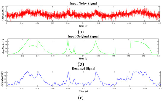
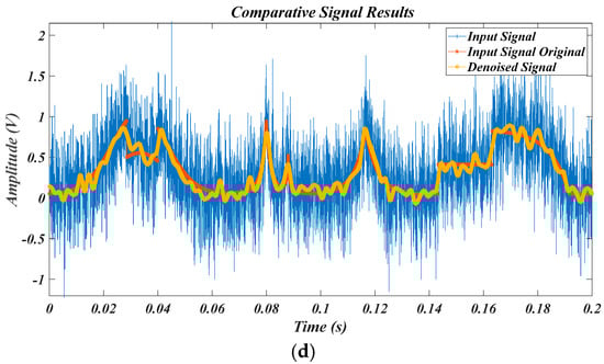
Figure 12. Comparative waveforms of L3 under SNR = 1 dB: (a) noisy input signal, (b) original input signal, (c) denoised signal, (d) comparative signal results.

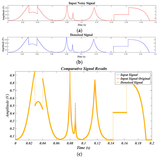
Figure 13. Comparative waveforms of L3 under SNR = 50 dB, (a) input noisy signal, (b) denoised signal, (c) comparative signal results.

Table 7 shows the performances based on SNR, MSE, RMSE, Corr, ${SNR}_{imp}$, ${RMSE}_{imp}$, ${MSE}_{imp}$, and ${Corr}_{imp}$ under different noise levels in the range of 1 dB to 50 dB. The ${SNR}_{denoised}$ results increase with the SNR level, which provides some improvement in ${SNR}_{imp}$. This is also true for Corr and ${Corr}_{imp}$ which converge to one and are superior. In contrast, this table reveals the decremental MSE and RMSE results, which approach zero. Improvements, such as ${RMSE}_{imp}$, and ${MSE}_{imp}$ are preferable. In conclusion, the proposed method exhibits strong potential for practical implementation, as evidenced by the substantial improvements observed across multiple evaluation criteria. Notably, the method achieves correlation levels nearing 100% across a broad range of SNR values, ensures a minimum SNR gain of 21% as given in Table 7, and delivers denoised signals that closely resemble the original waveforms, an outcome clearly illustrated in Figure 12 and Figure 13. These results validate the robustness and effectiveness of the approach under varying noise conditions.

Table 7. Metric results for L3.

${\mathit{S}\mathit{N}\mathit{R}}_{\mathit{n}\mathit{o}\mathit{i}\mathit{s}\mathit{y}}$	${\mathit{S}\mathit{N}\mathit{R}}_{\mathit{d}\mathit{e}\mathit{n}\mathit{o}\mathit{i}\mathit{s}\mathit{e}\mathit{d}}$	${\mathit{S}\mathit{N}\mathit{R}}_{\mathit{i}\mathit{m}\mathit{p}}$ (%)	${\mathit{R}\mathit{M}\mathit{S}\mathit{E}}_{\mathit{n}\mathit{o}\mathit{i}\mathit{s}\mathit{y}}$	${\mathit{R}\mathit{M}\mathit{S}\mathit{E}}_{\mathit{d}\mathit{e}\mathit{n}\mathit{o}\mathit{i}\mathit{s}\mathit{e}\mathit{d}}$	${\mathit{R}\mathit{M}\mathit{S}\mathit{E}}_{\mathit{i}\mathit{m}\mathit{p}}$ (%)	${\mathit{M}\mathit{S}\mathit{E}}_{\mathit{n}\mathit{o}\mathit{i}\mathit{s}\mathit{y}}$	${\mathit{M}\mathit{S}\mathit{E}}_{\mathit{d}\mathit{e}\mathit{n}\mathit{o}\mathit{i}\mathit{s}\mathit{e}\mathit{d}}$	${\mathit{M}\mathit{S}\mathit{E}}_{\mathit{i}\mathit{m}\mathit{p}}$ (%)	${\mathit{C}\mathit{o}\mathit{r}\mathit{r}}_{\mathit{n}\mathit{o}\mathit{i}\mathit{s}\mathit{y}}$	${\mathit{C}\mathit{o}\mathit{r}\mathit{r}}_{\mathit{d}\mathit{e}\mathit{n}\mathit{o}\mathit{i}\mathit{s}\mathit{e}\mathit{d}}$	${\mathit{C}\mathit{o}\mathit{r}\mathit{r}}_{\mathit{i}\mathit{m}\mathit{p}}$ (%)
1	18.173	1773.480	0.368	0.051	86.159	0.136	0.003	98.084	0.587	0.981	66.961
2	18.662	1766.208	0.335	0.048	85.605	0.112	0.002	97.928	0.613	0.983	60.218
3	18.531	826.528	0.296	0.049	83.482	0.088	0.002	97.272	0.656	0.982	49.815
4	19.407	546.912	0.259	0.044	82.914	0.067	0.002	97.081	0.710	0.985	38.822
5	20.357	408.930	0.231	0.040	82.823	0.053	0.002	97.049	0.737	0.988	34.124
10	23.596	162.177	0.132	0.027	79.280	0.017	0.001	95.707	0.893	0.995	11.422
15	27.245	94.608	0.074	0.018	75.704	0.005	0.000	94.097	0.961	0.998	3.849
20	31.507	65.828	0.041	0.011	73.167	0.002	0.000	92.800	0.988	0.999	1.155
25	36.902	53.756	0.023	0.006	74.653	0.001	0.000	93.575	0.996	1.000	0.381
30	40.810	40.723	0.013	0.004	71.768	0.000	0.000	92.030	0.999	1.000	0.123
35	45.436	33.636	0.007	0.002	69.718	0.000	0.000	90.830	1.000	1.000	0.036
40	49.799	27.690	0.004	0.001	68.381	0.000	0.000	90.002	1.000	1.000	0.012
45	54.955	24.899	0.002	0.001	68.024	0.000	0.000	89.775	1.000	1.000	0.004
50	59.126	20.666	0.001	0.000	65.128	0.000	0.000	87.839	1.000	1.000	0.001

The final results for this signal, obtained using the best-performing denoising models, are presented in Table 8. The level of denoising is mostly higher than “5” for all noise levels, and is distinct from the signal in $x\left(t\right)$ signal in Equation (11). Although the models incorporate a threshold rule, denoising methods based on Mean and Bayes parameters perform the best across most noise levels, while the optimal wavelet type varies depending on the noise level. This indicates that the wavelet type does not ensure the best performance, and the other deterministic parameters are more effective. These results differ from the other results for the signal in Equation (11).

Table 8. Best models per each SNR level for L3.

SNR (dB)	Level	Wavelet Type	Threshold Rule	Denoising Method	SNR (dB)	Level	Wavelet Type	Threshold Rule	Denoising Method	SNR (dB)	Level	Wavelet Type	Threshold Rule	Denoising Method
1	8	db4	Mean	Bayes	10	7	sym7	Mean	Bayes	35	6	bior4.4	Median	Bayes
2	7	db5	Mean	Bayes	15	7	sym6	Mean	Bayes	40	6	coif2	Median	Bayes
3	8	sym3	Soft	SURE	20	8	coif1	Mean	Bayes	45	9	bior4.4	Median	Bayes
4	7	sym3	Mean	Bayes	25	6	coif2	Mean	Bayes	50	8	sym4	Median	Bayes
5	8	fk18	Soft	SURE	30	6	bior4.4	Median	Bayes

As seen in Figure 14, for normal ECG signals, the models performed well under high-SNR noise levels (e.g., 30 and 50 dB), and also yielded quite consistent results at low SNR levels like 1 dB. Figure 15 shows that while the performance was quite good at SNR levels of 30–50 dB, it was observed that it made oscillatory predictions of abnormal points under very low SNR levels of 1 dB, i.e., high, intense noise. The low amplitude and duration changes in the high noise environment contributed to this error.

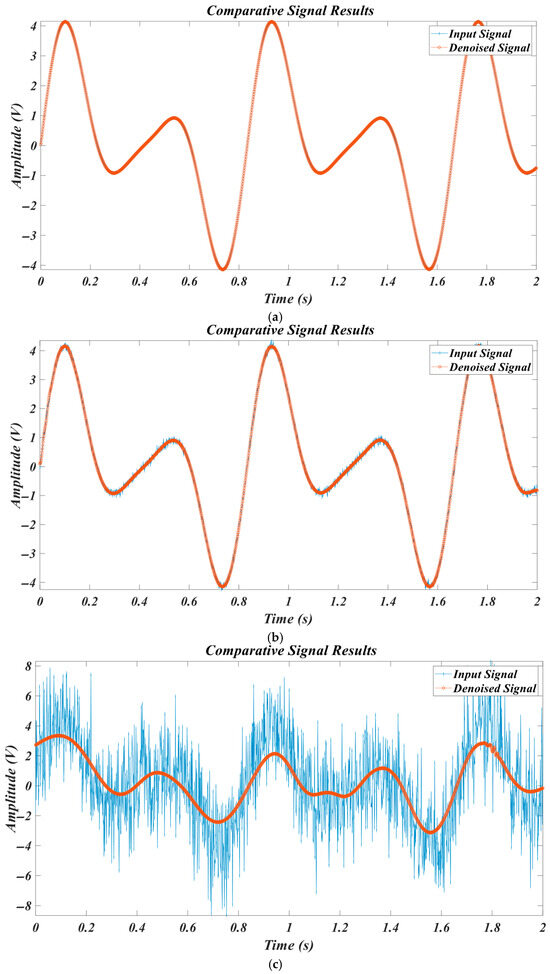
Figure 14. Results for normal ECG signals under (a) 50 dB, (b) 30 dB, (c) 1 dB.

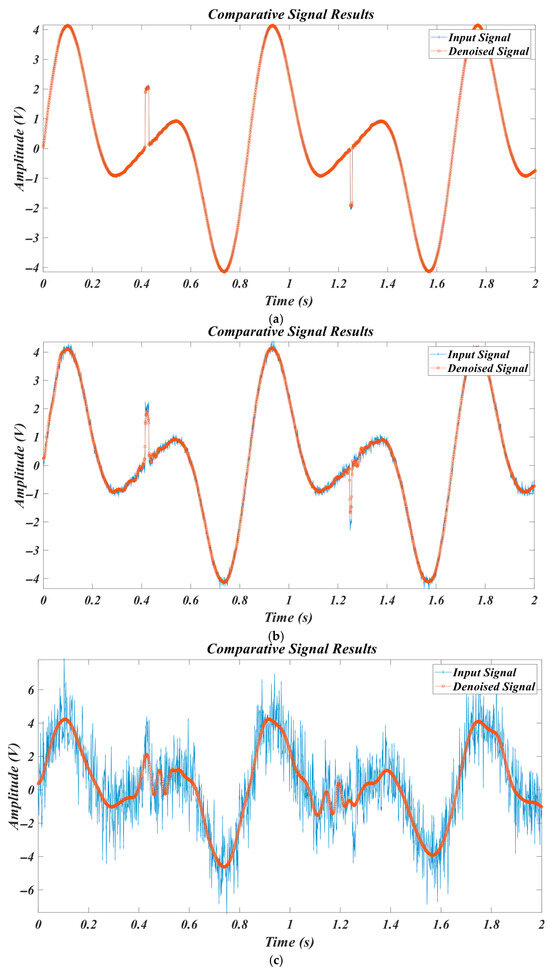
Figure 15. Results for abnormal ECG signals under (a) 50 dB, (b) 30 dB, (c) 1 dB.

As seen in Table 9, the proposed method yields successful results for both normal and abnormal ECG signals. Due to the inherent temporary effects of an abnormal ECG, it can be said that it yields relatively lower results than a normal ECG. However, overall, the proposed method yielded successful results.

Table 9. Comparative results for normal vs. abnormal.

	Normal ECG		Abnormal ECG
${\mathit{S}\mathit{N}\mathit{R}}_{\mathit{n}\mathit{o}\mathit{i}\mathit{s}\mathit{y}}$ (dB)	${\mathit{S}\mathit{N}\mathit{R}}_{\mathit{d}\mathit{e}\mathit{n}\mathit{o}\mathit{i}\mathit{s}\mathit{e}\mathit{d}}$ (dB)	${\mathit{S}\mathit{N}\mathit{R}}_{\mathit{i}\mathit{m}\mathit{p}}$ (%)	${\mathit{S}\mathit{N}\mathit{R}}_{\mathit{d}\mathit{e}\mathit{n}\mathit{o}\mathit{i}\mathit{s}\mathit{e}\mathit{d}}$ (dB)	${\mathit{S}\mathit{N}\mathit{R}}_{\mathit{i}\mathit{m}\mathit{p}}$ (%)
1	9.22	822	8.16	716
5	20.01	300.2	18.10	262
10	19.56	95.6	15.57	55.7
20	32.95	64.75	22.07	10.35
30	42.03	40.1	31.35	4.5
40	50.37	25.93	40.98	2.45
50	56.91	13.82	54.27	8.54

4.2.3. Results for $L4$ for Different SNR Levels

Another signal to be obtained is the $x\left(t\right)$ signal in Equation (11) in [40]. Processes similar to those used for the other signals were implemented for this signal. Signals with SNR levels of 1 dB and 50 dB are shown in Figure 16 and Figure 17, respectively. A difference in the compatibility of the original signal can be explicitly observed in the figures.

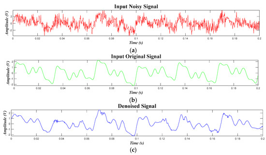
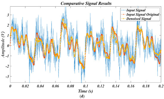
Figure 16. Comparative waveforms of L4 under SNR = 1 dB: (a) noisy input signal, (b) input original input signal, (c) denoised signal, (d) comparative signal results.

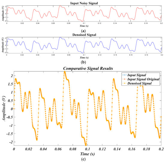
Figure 17. Comparative waveforms of L4 under SNR = 50 dB: (a) noisy input signal, (b) denoised signal, and (c) comparative signal results.

Table 10 lists comparative results for SNR, MSE, RMSE, Corr, ${SNR}_{imp}$, ${RMSE}_{imp}$, ${MSE}_{imp}$, and ${Corr}_{imp}$ under noise levels between 1 dB and 50 dB. The ${SNR}_{denoised}$ results are increased by raising the SNR level, which gives an advantage for ${SNR}_{imp},$ as in the results of the signals above. Moreover, the details of Corr, ${Corr}_{imp}$, ${RMSE}_{imp}$, ${MSE}_{imp}$, ${RMSE}_{imp}$, and ${MSE}_{imp}$ mentioned before are also true for the results of this signal. In conclusion, the proposed method demonstrates considerable promise and practical applicability, as evidenced by the improvements reported in Table 10, highlighting a minimum of 11% SNR enhancement and a high correlation consistency approaching 100% across various SNR levels. Furthermore, the strong visual similarity between the denoised and original signals, as illustrated in Figure 16 and Figure 17, further supports the robustness and effectiveness of the approach for diverse noise cases.

Table 10. Metric results for L4.

${\mathit{S}\mathit{N}\mathit{R}}_{\mathit{n}\mathit{o}\mathit{i}\mathit{s}\mathit{y}}$	${\mathit{S}\mathit{N}\mathit{R}}_{\mathit{d}\mathit{e}\mathit{n}\mathit{o}\mathit{i}\mathit{s}\mathit{e}\mathit{d}}$	${\mathit{S}\mathit{N}\mathit{R}}_{\mathit{i}\mathit{m}\mathit{p}}$ (%)	${\mathit{R}\mathit{M}\mathit{S}\mathit{E}}_{\mathit{n}\mathit{o}\mathit{i}\mathit{s}\mathit{y}}$	${\mathit{R}\mathit{M}\mathit{S}\mathit{E}}_{\mathit{d}\mathit{e}\mathit{n}\mathit{o}\mathit{i}\mathit{s}\mathit{e}\mathit{d}}$	${\mathit{R}\mathit{M}\mathit{S}\mathit{E}}_{\mathit{i}\mathit{m}\mathit{p}}$ (%)	${\mathit{M}\mathit{S}\mathit{E}}_{\mathit{n}\mathit{o}\mathit{i}\mathit{s}\mathit{y}}$	${\mathit{M}\mathit{S}\mathit{E}}_{\mathit{d}\mathit{e}\mathit{n}\mathit{o}\mathit{i}\mathit{s}\mathit{e}\mathit{d}}$	${\mathit{M}\mathit{S}\mathit{E}}_{\mathit{i}\mathit{m}\mathit{p}}$ (%)	${\mathit{C}\mathit{o}\mathit{r}\mathit{r}}_{\mathit{n}\mathit{o}\mathit{i}\mathit{s}\mathit{y}}$	${\mathit{C}\mathit{o}\mathit{r}\mathit{r}}_{\mathit{d}\mathit{e}\mathit{n}\mathit{o}\mathit{i}\mathit{s}\mathit{e}\mathit{d}}$	${\mathit{C}\mathit{o}\mathit{r}\mathit{r}}_{\mathit{i}\mathit{m}\mathit{p}}$ (%)
1	11.312	1031.184	0.918	0.282	69.311	0.844	0.079	90.582	0.750	0.963	28.421
2	13.120	556.006	0.797	0.229	71.264	0.634	0.052	91.742	0.791	0.975	23.283
3	11.996	299.851	0.769	0.261	66.125	0.592	0.068	88.525	0.807	0.970	20.140
4	14.037	250.918	0.663	0.206	68.938	0.440	0.042	90.351	0.846	0.980	15.846
5	14.858	197.161	0.575	0.187	67.430	0.331	0.035	89.392	0.874	0.985	12.631
10	19.487	94.873	0.321	0.110	65.740	0.103	0.012	88.262	0.956	0.995	4.033
15	24.629	64.192	0.179	0.061	65.979	0.032	0.004	88.426	0.985	0.998	1.314
20	28.318	41.588	0.103	0.040	61.339	0.011	0.002	85.053	0.995	0.999	0.420
25	32.956	31.822	0.055	0.023	57.559	0.003	0.001	81.987	0.999	1.000	0.116
30	36.808	22.694	0.032	0.015	53.240	0.001	0.000	78.135	1.000	1.000	0.037
35	41.155	17.586	0.019	0.009	51.315	0.000	0.000	76.298	1.000	1.000	0.012
40	45.605	14.013	0.011	0.005	50.137	0.000	0.000	75.137	1.000	1.000	0.004
45	49.865	10.811	0.006	0.003	45.152	0.000	0.000	69.917	1.000	1.000	0.001
50	55.655	11.310	0.003	0.002	47.682	0.000	0.000	72.629	1.000	1.000	0.000

The final results for this signal with the best denoising models are given in Table 11. Unlike the models for other signal types, no parameter exhibited the best denoising performance for this signal. The denoising model changed according to signal type and noise level.

Table 11. Best models per SNR level for L4.

SNR (dB)	Level	Wavelet Type	Threshold Rule	Denoising Method	SNR (dB)	Level	Wavelet Type	Threshold Rule	Denoising Method	SNR (dB)	Level	Wavelet Type	Threshold Rule	Denoising Method
1	6	db7	Soft	SURE	10	9	sym7	Soft	Bayes	35	3	sym7	Mean	Bayes
2	5	fk22	Soft	SURE	15	3	fk22	James-Stein	BlockJS	40	3	db8	Median	Bayes
3	9	sym7	Soft	SURE	20	3	fk14	James-Stein	BlockJS	45	2	coif4	Hard	FDR
4	7	fk18	Mean	Bayes	25	3	fk22	James-Stein	BlockJS	50	2	db8	James-Stein	BlockJS
5	3	coif4	James-Stein	BlockJS	30	9	db8	Mean	Bayes

4.3. Results for Synthetic Data of PQDs

In this section, sinusoidal signals are shown in Table 2 for a 1 V amplitude and 50 Hz frequency in the interval of 49.5 Hz and 50.5 Hz, and different noise injections from 1 dB to 50 dB SNR. Since the test signals with the original signal input under 1 dB noise and the ones without the original signal input under 50 dB noise were mentioned in detail above, similar test signals will be shown comparatively in a single figure here.

Case 1, a pure signal under 1 dB noise, is shown in Figure 18. The noise of the noisy input signal is reduced as much as possible, although it is highly noisy. The denoised signal is in harmony with the original signal, with some small errors. The other signal under 50 dB noise, which is almost noiseless, is revealed in Figure 19. Noisy and denoised signals are in phase in the figures.

Figure 18. Comparative waveforms of Case 1 of L5 under SNR = 1 dB.

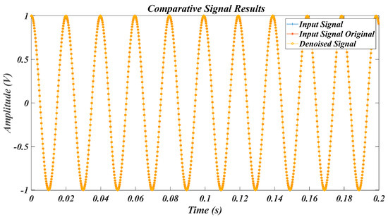
Figure 19. Comparative waveforms of Case 1 of L5 under SNR = 50 dB.

Table 11 indicates the performances based on SNR, MSE, RMSE, Corr, ${SNR}_{imp}$, ${RMSE}_{imp}$, ${MSE}_{imp}$, and ${Corr}_{imp}$ under different noise levels in the interval of 1 dB to 50 dB. The ${SNR}_{denoised}$ results increase with the SNR level, which brings some improvement in ${SNR}_{imp}$. This is also true for Corr and ${Corr}_{imp}$ which converge to one and are superior. In contrast, this table reveals decremental MSE and RMSE results, which approach zero. Improvements in parameters such as ${RMSE}_{imp}$, and ${MSE}_{imp}$ are preferable. The proposed method demonstrates strong applicability, as evidenced by the correlation consistency nearing 100% across various SNR levels and a minimum SNR enhancement of 11% as shown in Table 12. Moreover, the visual alignment of the denoised and original signals in Figure 15 and Figure 16 reinforces the effectiveness of the approach. The final results for the signal in Case 1 are the best denoising models given in Table 13. The level of denoising is mostly higher than “4” versus the noise levels. For models with the threshold rule, denoising method parameters consisting of mean and Bayes are the best at most noise levels, and the parameter of wavelet type is variable for different noise levels. This proves that the wavelet type does not ensure the best performance, and the other deterministic parameters are more effective.

Table 12. Metric results for the synthetic signal in Case 1 of L5.

${\mathit{S}\mathit{N}\mathit{R}}_{\mathit{n}\mathit{o}\mathit{i}\mathit{s}\mathit{y}}$	${\mathit{S}\mathit{N}\mathit{R}}_{\mathit{d}\mathit{e}\mathit{n}\mathit{o}\mathit{i}\mathit{s}\mathit{e}\mathit{d}}$	${\mathit{S}\mathit{N}\mathit{R}}_{\mathit{i}\mathit{m}\mathit{p}}$ (%)	${\mathit{R}\mathit{M}\mathit{S}\mathit{E}}_{\mathit{n}\mathit{o}\mathit{i}\mathit{s}\mathit{y}}$	${\mathit{R}\mathit{M}\mathit{S}\mathit{E}}_{\mathit{d}\mathit{e}\mathit{n}\mathit{o}\mathit{i}\mathit{s}\mathit{e}\mathit{d}}$	${\mathit{R}\mathit{M}\mathit{S}\mathit{E}}_{\mathit{i}\mathit{m}\mathit{p}}$ (%)	${\mathit{M}\mathit{S}\mathit{E}}_{\mathit{n}\mathit{o}\mathit{i}\mathit{s}\mathit{y}}$	${\mathit{M}\mathit{S}\mathit{E}}_{\mathit{d}\mathit{e}\mathit{n}\mathit{o}\mathit{i}\mathit{s}\mathit{e}\mathit{d}}$	${\mathit{M}\mathit{S}\mathit{E}}_{\mathit{i}\mathit{m}\mathit{p}}$ (%)	${\mathit{C}\mathit{o}\mathit{r}\mathit{r}}_{\mathit{n}\mathit{o}\mathit{i}\mathit{s}\mathit{y}}$	${\mathit{C}\mathit{o}\mathit{r}\mathit{r}}_{\mathit{d}\mathit{e}\mathit{n}\mathit{o}\mathit{i}\mathit{s}\mathit{e}\mathit{d}}$	${\mathit{C}\mathit{o}\mathit{r}\mathit{r}}_{\mathit{i}\mathit{m}\mathit{p}}$ (%)
1	11.312	1031.184	0.918	0.282	69.311	0.844	0.079	90.582	0.750	0.963	28.421
2	13.120	556.006	0.797	0.229	71.264	0.634	0.052	91.742	0.791	0.975	23.283
3	11.996	299.851	0.769	0.261	66.125	0.592	0.068	88.525	0.807	0.970	20.140
4	14.037	250.918	0.663	0.206	68.938	0.440	0.042	90.351	0.846	0.980	15.846
5	14.858	197.161	0.575	0.187	67.430	0.331	0.035	89.392	0.874	0.985	12.631
10	19.487	94.873	0.321	0.110	65.740	0.103	0.012	88.262	0.956	0.995	4.033
15	24.629	64.192	0.179	0.061	65.979	0.032	0.004	88.426	0.985	0.998	1.314
20	28.318	41.588	0.103	0.040	61.339	0.011	0.002	85.053	0.995	0.999	0.420
25	32.956	31.822	0.055	0.023	57.559	0.003	0.001	81.987	0.999	1.000	0.116
30	36.808	22.694	0.032	0.015	53.240	0.001	0.000	78.135	1.000	1.000	0.037
35	41.155	17.586	0.019	0.009	51.315	0.000	0.000	76.298	1.000	1.000	0.012
40	45.605	14.013	0.011	0.005	50.137	0.000	0.000	75.137	1.000	1.000	0.004
45	49.865	10.811	0.006	0.003	45.152	0.000	0.000	69.917	1.000	1.000	0.001
50	55.655	11.310	0.003	0.002	47.682	0.000	0.000	72.629	1.000	1.000	0.000

Table 13. Best models for each SNR level for the Synthetic Signal in Case 1 of L5.

SNR (dB)	Level	Wavelet Type	Threshold Rule	Denoising Method	SNR (dB)	Level	Wavelet Type	Threshold Rule	Denoising Method	SNR (dB)	Level	Wavelet Type	Threshold Rule	Denoising Method
1	5	coif5	James-Stein	BlockJS	10	5	fk22	Soft	SURE	35	4	sym8	Soft	Bayes
2	9	fk18	Soft	Bayes	15	5	coif4	Median	Bayes	40	4	db9	Hard	FDR
3	5	fk22	James-Stein	BlockJS	20	9	bior6.8	Soft	Bayes	45	4	db10	Median	Bayes
4	6	fk22	Hard	Bayes	25	8	db9	Hard	FDR	50	6	db10	James-Stein	BlockJS
5	5	fk18	James-Stein	BlockJS	30	4	sym8	Soft	Bayes

Figure 20 presents Case 2, where a sag-type signal is contaminated with 1 dB of noise. Despite the high noise level, the input signal is effectively denoised, showing minimal deviation from the clean reference signal. In comparison, the signal with 50 dB noise, depicted in Figure 21, exhibits almost no degradation and closely matches the original. Both noisy and denoised signals maintain phase coherence.

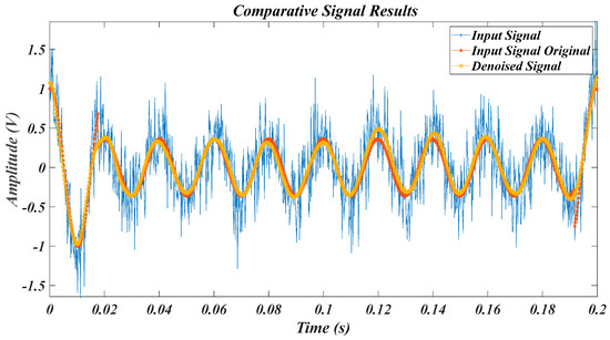
Figure 20. Comparative waveforms of Case 2 of L5 under SNR = 1 dB.

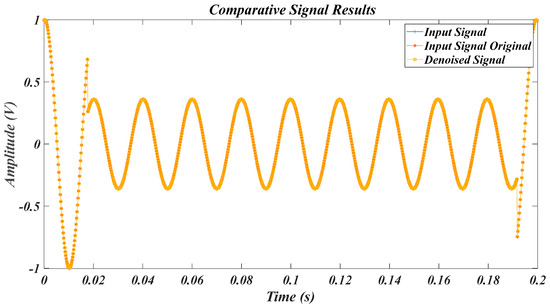
Figure 21. Comparative waveforms of Case 2 of L5 under SNR = 50 dB.

Table 14 summarizes the performance metrics across varying noise levels in the range of 1–50 dB, showing improvement in ${SNR}_{denoised}$ and ${Corr}_{imp}$, while MSE and RMSE progressively decrease, approaching zero. These results confirm that ${RMSE}_{imp}$ and ${MSE}_{imp}$ values improve with increasing SNR. The results indicate that the method achieves a minimum SNR improvement of 15% as shown in Table 13, and maintains nearly perfect correlation across different noise levels. The visual conformity between the output and original signals in Figure 20 and Figure 21 further highlights its practical potential. Table 15 reports the optimal denoising models for Case 2. Most models achieve a denoising level above 4 across all noise levels. Threshold-based methods with median or Bayes estimation perform best overall, while the choice of wavelet type shows variable effectiveness, indicating that it is less deterministic in its overall performance.

Table 14. Metric results for the synthetic signal in Case 2 of L5.

${\mathit{S}\mathit{N}\mathit{R}}_{\mathit{n}\mathit{o}\mathit{i}\mathit{s}\mathit{y}}$	${\mathit{S}\mathit{N}\mathit{R}}_{\mathit{d}\mathit{e}\mathit{n}\mathit{o}\mathit{i}\mathit{s}\mathit{e}\mathit{d}}$	${\mathit{S}\mathit{N}\mathit{R}}_{\mathit{i}\mathit{m}\mathit{p}}$ (%)	${\mathit{R}\mathit{M}\mathit{S}\mathit{E}}_{\mathit{n}\mathit{o}\mathit{i}\mathit{s}\mathit{y}}$	${\mathit{R}\mathit{M}\mathit{S}\mathit{E}}_{\mathit{d}\mathit{e}\mathit{n}\mathit{o}\mathit{i}\mathit{s}\mathit{e}\mathit{d}}$	${\mathit{R}\mathit{M}\mathit{S}\mathit{E}}_{\mathit{i}\mathit{m}\mathit{p}}$ (%)	${\mathit{M}\mathit{S}\mathit{E}}_{\mathit{n}\mathit{o}\mathit{i}\mathit{s}\mathit{y}}$	${\mathit{M}\mathit{S}\mathit{E}}_{\mathit{d}\mathit{e}\mathit{n}\mathit{o}\mathit{i}\mathit{s}\mathit{e}\mathit{d}}$	${\mathit{M}\mathit{S}\mathit{E}}_{\mathit{i}\mathit{m}\mathit{p}}$ (%)	${\mathit{C}\mathit{o}\mathit{r}\mathit{r}}_{\mathit{n}\mathit{o}\mathit{i}\mathit{s}\mathit{y}}$	${\mathit{C}\mathit{o}\mathit{r}\mathit{r}}_{\mathit{d}\mathit{e}\mathit{n}\mathit{o}\mathit{i}\mathit{s}\mathit{e}\mathit{d}}$	${\mathit{C}\mathit{o}\mathit{r}\mathit{r}}_{\mathit{i}\mathit{m}\mathit{p}}$ (%)
1	13.628	1262.772	0.305	0.071	76.664	0.093	0.005	94.555	0.768	0.979	27.544
2	15.166	658.303	0.272	0.060	78.081	0.074	0.004	95.195	0.782	0.985	25.951
3	15.150	404.997	0.246	0.060	75.748	0.061	0.004	94.118	0.814	0.985	20.956
4	15.182	279.539	0.206	0.059	71.127	0.042	0.004	91.664	0.850	0.985	15.810
5	19.629	292.577	0.183	0.036	80.551	0.034	0.001	96.217	0.878	0.995	13.303
10	19.554	95.542	0.114	0.036	68.518	0.013	0.001	90.089	0.949	0.995	4.766
15	24.535	63.567	0.062	0.020	67.326	0.004	0.000	89.324	0.984	0.998	1.423
20	29.984	49.919	0.034	0.011	68.307	0.001	0.000	89.956	0.995	0.999	0.448
25	33.828	35.310	0.019	0.007	64.166	0.000	0.000	87.159	0.998	1.000	0.141
30	38.917	29.722	0.011	0.004	64.357	0.000	0.000	87.296	0.999	1.000	0.044
35	43.295	23.701	0.006	0.002	61.849	0.000	0.000	85.445	1.000	1.000	0.014
40	48.150	20.374	0.003	0.001	60.618	0.000	0.000	84.491	1.000	1.000	0.004
45	52.685	17.078	0.002	0.001	57.359	0.000	0.000	81.817	1.000	1.000	0.001
50	57.344	14.688	0.001	0.000	57.374	0.000	0.000	81.830	1.000	1.000	0.000

Table 15. Best models for each SNR level for the synthetic signal in Case 2 of L5.

SNR (dB)	Level	Wavelet Type	Threshold Rule	Denoising Method	SNR (dB)	Level	Wavelet Type	Threshold Rule	Denoising Method	SNR (dB)	Level	Wavelet Type	Threshold Rule	Denoising Method
1	6	fk22	James-Stein	BlockJS	10	5	sym8	Mean	Bayes	35	4	db6	Median	Bayes
2	5	fk22	Hard	FDR	15	6	coif5	Mean	Bayes	40	4	db8	Hard	UT
3	6	coif5	Soft	Bayes	20	4	sym7	Hard	UT	45	7	coif4	Median	Bayes
4	9	sym8	Hard	Bayes	25	4	sym6	Median	Bayes	50	3	bior5.5	Median	Bayes
5	5	coif5	Soft	Bayes	30	4	bior5.5	Mean	Bayes

In Case 3, shown in Figure 22, a swell signal corrupted by 1 dB of noise is processed. The denoised version effectively suppresses noise, maintaining close alignment with the reference waveform. Conversely, the case under 50 dB noise, shown in Figure 23, reveals minimal distortion, with noisy and denoised signals being nearly indistinguishable and in phase. It can be concluded that the proposed algorithm is both promising and applicable, given the significant metric improvements, particularly the correlation values approaching 100%, and the minimum of 16% SNR gain presented in Table 16. The visual comparisons in Figure 22 and Figure 23 further substantiate this claim. Performance metrics in Table 16 demonstrate that higher input SNR leads to increased ${SNR }_{denoised}$ and ${Corr}_{imp}$ values, whereas RMSE and MSE consistently drop toward zero. This trend confirms that noise suppression improves with signal clarity. Table 17 highlights the best denoising models for Case 3, where thresholding and wavelet rules paired with Hard and Bayes parameters generally yield the highest performance. The wavelet selection, however, does not consistently influence the results, emphasizing the dominance of other model parameters.

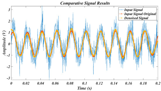
Figure 22. Comparative waveforms of Case 3 of L5 under SNR = 1 dB.

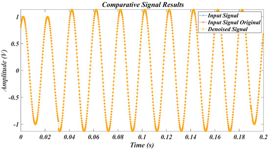
Figure 23. Comparative waveforms of Case 3 of L5 under SNR = 50 dB.

Table 16. Metric results for the synthetic signal in Case 3 of L5.

${\mathit{S}\mathit{N}\mathit{R}}_{\mathit{n}\mathit{o}\mathit{i}\mathit{s}\mathit{y}}$	${\mathit{S}\mathit{N}\mathit{R}}_{\mathit{d}\mathit{e}\mathit{n}\mathit{o}\mathit{i}\mathit{s}\mathit{e}\mathit{d}}$	${\mathit{S}\mathit{N}\mathit{R}}_{\mathit{i}\mathit{m}\mathit{p}}$ (%)	${\mathit{R}\mathit{M}\mathit{S}\mathit{E}}_{\mathit{n}\mathit{o}\mathit{i}\mathit{s}\mathit{y}}$	${\mathit{R}\mathit{M}\mathit{S}\mathit{E}}_{\mathit{d}\mathit{e}\mathit{n}\mathit{o}\mathit{i}\mathit{s}\mathit{e}\mathit{d}}$	${\mathit{R}\mathit{M}\mathit{S}\mathit{E}}_{\mathit{i}\mathit{m}\mathit{p}}$ (%)	${\mathit{M}\mathit{S}\mathit{E}}_{\mathit{n}\mathit{o}\mathit{i}\mathit{s}\mathit{y}}$	${\mathit{M}\mathit{S}\mathit{E}}_{\mathit{d}\mathit{e}\mathit{n}\mathit{o}\mathit{i}\mathit{s}\mathit{e}\mathit{d}}$	${\mathit{M}\mathit{S}\mathit{E}}_{\mathit{i}\mathit{m}\mathit{p}}$ (%)	${\mathit{C}\mathit{o}\mathit{r}\mathit{r}}_{\mathit{n}\mathit{o}\mathit{i}\mathit{s}\mathit{y}}$	${\mathit{C}\mathit{o}\mathit{r}\mathit{r}}_{\mathit{d}\mathit{e}\mathit{n}\mathit{o}\mathit{i}\mathit{s}\mathit{e}\mathit{d}}$	${\mathit{C}\mathit{o}\mathit{r}\mathit{r}}_{\mathit{i}\mathit{m}\mathit{p}}$ (%)
1	17.681	1668.115	0.673	0.102	84.863	0.453	0.010	97.709	0.759	0.992	30.724
2	16.680	733.990	0.608	0.114	81.200	0.370	0.013	96.466	0.796	0.990	24.255
3	16.009	433.625	0.566	0.123	78.198	0.321	0.015	95.247	0.806	0.988	22.483
4	20.559	413.969	0.475	0.073	84.606	0.226	0.005	97.630	0.855	0.996	16.446
5	19.613	292.258	0.433	0.082	81.154	0.187	0.007	96.448	0.869	0.995	14.516
10	23.952	139.519	0.242	0.049	79.532	0.058	0.002	95.811	0.956	0.998	4.431
15	26.554	77.029	0.140	0.037	73.720	0.019	0.001	93.094	0.984	0.999	1.476
20	30.586	52.928	0.076	0.023	69.855	0.006	0.001	90.913	0.995	1.000	0.441
25	36.696	46.783	0.045	0.011	74.373	0.002	0.000	93.433	0.998	1.000	0.153
30	39.646	32.152	0.025	0.008	67.440	0.001	0.000	89.398	0.999	1.000	0.046
35	43.957	25.592	0.014	0.005	65.009	0.000	0.000	87.756	1.000	1.000	0.014
40	47.795	19.487	0.008	0.003	58.212	0.000	0.000	82.538	1.000	1.000	0.004
45	51.881	15.290	0.004	0.002	55.823	0.000	0.000	80.484	1.000	1.000	0.001
50	58.034	16.068	0.002	0.001	60.615	0.000	0.000	84.488	1.000	1.000	0.000

Table 17. Best models for each SNR level for the synthetic signal in Case 3 of L5.

SNR (dB)	Level	Wavelet Type	Threshold Rule	Denoising Method	SNR (dB)	Level	Wavelet Type	Threshold Rule	Denoising Method	SNR (dB)	Level	Wavelet Type	Threshold Rule	Denoising Method
1	6	fk22	Soft	Bayes	10	5	fk22	Hard	FDR	35	4	coif4	Hard	UT
2	9	fk22	Median	Bayes	15	8	fk18	Soft	Bayes	40	5	sym7	Median	Bayes
3	6	fk14	James-Stein	BlockJS	20	5	sym8	James-Stein	BlockJS	45	4	db9	Mean	Bayes
4	8	fk22	Soft	Bayes	25	4	coif4	Hard	FDR	50	3	bior6.8	Hard	UT
5	6	fk22	Hard	Bayes	30	4	coif4	Hard	UT

As illustrated in Figure 24, the flicker signal in Case 4 was subjected to 1 dB of noise. The effective noise suppression technique significantly enhances signal clarity, as evidenced by the close match between the denoised and original waveforms in the figure. When the same signal is tested under 50 dB of noise in Figure 25, the negligible noise allows the denoised output to remain nearly identical to the original, with preserved phase alignment.

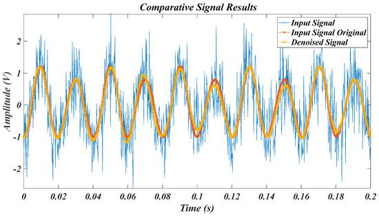
Figure 24. Comparative waveforms of Case 4 of L5 under SNR = 1 dB.

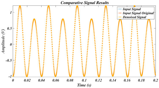
Figure 25. Comparative waveforms of Case 4 of L5 under SNR = 50 dB.

Table 18 captures how increasing the SNR improves the denoising output. ${SNR}_{denoised}$ and ${Corr}_{imp}$ increase steadily, while MSE and RMSE decrease. The resulting improvement in metrics like ${RMSE}_{imp}$ and ${MSE}_{imp}$ demonstrates the method’s robustness. It can be concluded that the proposed algorithm is both promising and applicable, given the significant metric improvements, particularly the correlation values approaching 100%, and the minimum 11% SNR gain presented in Table 18. Visual comparisons in Figure 24 and Figure 25 further substantiate this claim. Table 19 presents the highest-performing models for Case 4. Models incorporating James-Stein and Block JS thresholding and wavelet methods consistently perform best. The variation in wavelet types does not correlate strongly with performance, suggesting other parameters play a more critical role.

Table 18. Metric results for the synthetic signal in Case 4 of L5.

${\mathit{S}\mathit{N}\mathit{R}}_{\mathit{n}\mathit{o}\mathit{i}\mathit{s}\mathit{y}}$	${\mathit{S}\mathit{N}\mathit{R}}_{\mathit{d}\mathit{e}\mathit{n}\mathit{o}\mathit{i}\mathit{s}\mathit{e}\mathit{d}}$	${\mathit{S}\mathit{N}\mathit{R}}_{\mathit{i}\mathit{m}\mathit{p}}$ (%)	${\mathit{R}\mathit{M}\mathit{S}\mathit{E}}_{\mathit{n}\mathit{o}\mathit{i}\mathit{s}\mathit{y}}$	${\mathit{R}\mathit{M}\mathit{S}\mathit{E}}_{\mathit{d}\mathit{e}\mathit{n}\mathit{o}\mathit{i}\mathit{s}\mathit{e}\mathit{d}}$	${\mathit{R}\mathit{M}\mathit{S}\mathit{E}}_{\mathit{i}\mathit{m}\mathit{p}}$ (%)	${\mathit{M}\mathit{S}\mathit{E}}_{\mathit{n}\mathit{o}\mathit{i}\mathit{s}\mathit{y}}$	${\mathit{M}\mathit{S}\mathit{E}}_{\mathit{d}\mathit{e}\mathit{n}\mathit{o}\mathit{i}\mathit{s}\mathit{e}\mathit{d}}$	${\mathit{M}\mathit{S}\mathit{E}}_{\mathit{i}\mathit{m}\mathit{p}}$ (%)	${\mathit{C}\mathit{o}\mathit{r}\mathit{r}}_{\mathit{n}\mathit{o}\mathit{i}\mathit{s}\mathit{y}}$	${\mathit{C}\mathit{o}\mathit{r}\mathit{r}}_{\mathit{d}\mathit{e}\mathit{n}\mathit{o}\mathit{i}\mathit{s}\mathit{e}\mathit{d}}$	${\mathit{C}\mathit{o}\mathit{r}\mathit{r}}_{\mathit{i}\mathit{m}\mathit{p}}$ (%)
1	15.210	1421.003	0.650	0.124	80.947	0.422	0.015	96.370	0.734	0.985	34.242
2	16.242	712.119	0.572	0.110	80.773	0.327	0.012	96.303	0.782	0.988	26.418
3	15.647	421.561	0.511	0.118	76.960	0.261	0.014	94.692	0.811	0.987	21.762
4	19.009	375.237	0.449	0.080	82.207	0.202	0.006	96.834	0.853	0.995	16.541
5	17.836	256.725	0.406	0.091	77.459	0.165	0.008	94.919	0.876	0.993	13.285
10	21.865	118.650	0.234	0.058	75.408	0.055	0.003	93.952	0.950	0.997	4.964
15	26.766	78.438	0.128	0.033	74.399	0.016	0.001	93.446	0.984	0.999	1.506
20	32.002	60.008	0.072	0.018	75.131	0.005	0.000	93.816	0.995	1.000	0.475
25	38.275	53.100	0.040	0.009	78.139	0.002	0.000	95.221	0.998	1.000	0.148
30	42.229	40.762	0.023	0.006	75.831	0.001	0.000	94.158	0.999	1.000	0.048
35	47.040	34.401	0.013	0.003	74.730	0.000	0.000	93.614	1.000	1.000	0.014
40	51.500	28.751	0.007	0.002	72.605	0.000	0.000	92.495	1.000	1.000	0.004
45	55.398	23.107	0.004	0.001	70.432	0.000	0.000	91.258	1.000	1.000	0.002
50	59.120	18.241	0.002	0.001	64.279	0.000	0.000	87.240	1.000	1.000	0.000

Table 19. Best models for each SNR level for the synthetic signal in Case 4 of L5.

SNR (dB)	Level	Wavelet Type	Threshold Rule	Denoising Method	SNR (dB)	Level	Wavelet Type	Threshold Rule	Denoising Method	SNR (dB)	Level	Wavelet Type	Threshold Rule	Denoising Method
1	5	fk22	James-Stein	BlockJS	10	5	fk22	Median	Bayes	35	9	db9	Hard	FDR
2	5	fk22	James-Stein	BlockJS	15	4	bior6.8	James-Stein	BlockJS	40	7	coif5	James-Stein	BlockJS
3	9	db10	Soft	SURE	20	4	coif4	Soft	UT	45	4	db10	James-Stein	BlockJS
4	6	fk22	Soft	SURE	25	4	db9	Median	Bayes	50	3	db6	James-Stein	BlockJS
5	8	fk22	Soft	Bayes	30	7	db10	James-Stein	BlockJS

The denoising results of Case 5, affected by 1 dB—noise, are shown in Figure 26. Notably, the denoised signal exhibits minimal distortion and aligns closely with the original waveform. Similarly, under 50 dB noise, Figure 27, the signal remains virtually clean, with perfect phase agreement between noisy and denoised forms.

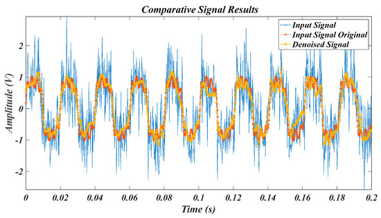
Figure 26. Comparative waveforms of Case 5 of L5 under SNR = 1 dB.

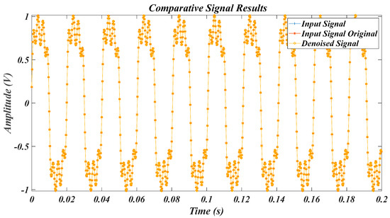
Figure 27. Comparative waveforms of Case 5 of L5 under SNR = 50 dB.

A performance evaluation, detailed in Table 20, reveals increasing ${SNR}_{denoised }$ and ${Corr}_{imp}$ with higher noise levels, while MSE and RMSE decrease accordingly. These improvements affirm the efficiency of the denoising technique across the SNR range. As evidenced by Table 20 and Figure 26 and Figure 27, the method yields substantial performance improvements, including a minimum 6% SNR gain and high correlation alignment with the reference signals. These findings underscore the approach’s viability for real-world applications. Table 21 outlines the best models for Case 5. Parameters like mean and Bayes consistently outperform others under high SNR levels, while in contrast, wavelet type shows no consistent advantage, highlighting the impact of parameter choice over transform base.

Table 20. Metric results for the synthetic signal in Case 5 of L5.

${\mathit{S}\mathit{N}\mathit{R}}_{\mathit{n}\mathit{o}\mathit{i}\mathit{s}\mathit{y}}$	${\mathit{S}\mathit{N}\mathit{R}}_{\mathit{d}\mathit{e}\mathit{n}\mathit{o}\mathit{i}\mathit{s}\mathit{e}\mathit{d}}$	${\mathit{S}\mathit{N}\mathit{R}}_{\mathit{i}\mathit{m}\mathit{p}}$ (%)	${\mathit{R}\mathit{M}\mathit{S}\mathit{E}}_{\mathit{n}\mathit{o}\mathit{i}\mathit{s}\mathit{y}}$	${\mathit{R}\mathit{M}\mathit{S}\mathit{E}}_{\mathit{d}\mathit{e}\mathit{n}\mathit{o}\mathit{i}\mathit{s}\mathit{e}\mathit{d}}$	${\mathit{R}\mathit{M}\mathit{S}\mathit{E}}_{\mathit{i}\mathit{m}\mathit{p}}$ (%)	${\mathit{M}\mathit{S}\mathit{E}}_{\mathit{n}\mathit{o}\mathit{i}\mathit{s}\mathit{y}}$	${\mathit{M}\mathit{S}\mathit{E}}_{\mathit{d}\mathit{e}\mathit{n}\mathit{o}\mathit{i}\mathit{s}\mathit{e}\mathit{d}}$	${\mathit{M}\mathit{S}\mathit{E}}_{\mathit{i}\mathit{m}\mathit{p}}$ (%)	${\mathit{C}\mathit{o}\mathit{r}\mathit{r}}_{\mathit{n}\mathit{o}\mathit{i}\mathit{s}\mathit{y}}$	${\mathit{C}\mathit{o}\mathit{r}\mathit{r}}_{\mathit{d}\mathit{e}\mathit{n}\mathit{o}\mathit{i}\mathit{s}\mathit{e}\mathit{d}}$	${\mathit{C}\mathit{o}\mathit{r}\mathit{r}}_{\mathit{i}\mathit{m}\mathit{p}}$ (%)
1	10.649	964.896	0.636	0.217	65.809	0.404	0.047	88.310	0.752	0.956	27.207
2	10.679	433.945	0.619	0.217	65.024	0.383	0.047	87.767	0.768	0.957	24.670
3	11.890	296.328	0.506	0.188	62.782	0.256	0.035	86.148	0.829	0.969	16.831
4	12.328	208.203	0.470	0.179	61.912	0.221	0.032	85.493	0.844	0.971	15.040
5	13.042	160.839	0.407	0.165	59.421	0.165	0.027	83.534	0.875	0.975	11.420
10	16.639	66.386	0.231	0.109	52.728	0.053	0.012	77.654	0.955	0.989	3.591
15	20.968	39.787	0.132	0.066	49.934	0.018	0.004	74.934	0.984	0.996	1.189
20	26.392	31.958	0.071	0.035	49.798	0.005	0.001	74.798	0.995	0.999	0.342
25	31.277	25.110	0.041	0.020	50.553	0.002	0.000	75.550	0.998	1.000	0.115
30	36.230	20.767	0.022	0.011	49.121	0.001	0.000	74.113	1.000	1.000	0.034
35	40.060	14.456	0.013	0.007	43.086	0.000	0.000	67.608	1.000	1.000	0.010
40	43.868	9.671	0.007	0.005	35.896	0.000	0.000	58.907	1.000	1.000	0.003
45	48.024	6.719	0.004	0.003	27.548	0.000	0.000	47.507	1.000	1.000	0.001
50	53.102	6.204	0.002	0.002	29.648	0.000	0.000	50.506	1.000	1.000	0.000

Table 21. Best models for each SNR level for the synthetic signal in Case 5 of L5.

SNR (dB)	Level	Wavelet Type	Threshold Rule	Denoising Method	SNR (dB)	Level	Wavelet Type	Threshold Rule	Denoising Method	SNR (dB)	Level	Wavelet Type	Threshold Rule	Denoising Method
1	9	coif2	Soft	SURE	10	9	fk14	Soft	SURE	35	2	coif5	James-Stein	BlockJS
2	9	sym7	Mean	Bayes	15	7	bior5.5	Hard	Bayes	40	2	coif5	Mean	Bayes
3	4	coif3	Soft	SURE	20	2	fk22	Soft	UT	45	3	db10	Mean	Bayes
4	6	sym3	Mean	Bayes	25	4	sym6	Median	Bayes	50	3	bior5.5	Median	Bayes
5	5	db9	Soft	SURE	30	2	coif5	James-Stein	BlockJS

Figure 28 illustrates Case 6 under 1 dB noise contamination, where effective denoising leads to be alike a signal without notches as seen in the figure. A different observation from the case under 1 dB of noise is made for the 50 dB case in Figure 29, where noise influence is negligible and in phase alignment is preserved.

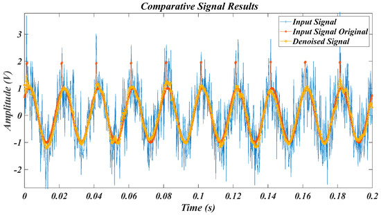
Figure 28. Comparative waveforms of Case 6 of L5 under SNR = 1 dB.

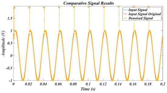
Figure 29. Comparative waveforms of Case 6 of L5 under SNR = 50 dB.

Table 22 analytically summarizes the impact of increasing SNR levels on denoising metrics. As expected, ${SNR}_{denoised }$ and ${Corr}_{imp}$ increase, approaching ideal values, while MSE and RMSE tend toward zero. These patterns confirm the effectiveness of the applied denoising strategy. Taken together, the quantitative improvements in correlation and SNR, specifically the 8.3% minimum SNR gain and near-perfect correlation across varying noise levels like in Table 12, alongside the waveform consistency in Figure 28 and Figure 29, provide strong evidence for the method’s practical utility. Table 23 identifies optimal models for Case 6, demonstrating that deterministic thresholding parameters like mean and Bayes significantly influence performance, whereas wavelet type does not consistently yield better outcomes, thereby downplaying its significance.

Table 22. Metric results for the synthetic signal in Case 6 of L5.

${\mathit{S}\mathit{N}\mathit{R}}_{\mathit{n}\mathit{o}\mathit{i}\mathit{s}\mathit{y}}$	${\mathit{S}\mathit{N}\mathit{R}}_{\mathit{d}\mathit{e}\mathit{n}\mathit{o}\mathit{i}\mathit{s}\mathit{e}\mathit{d}}$	${\mathit{S}\mathit{N}\mathit{R}}_{\mathit{i}\mathit{m}\mathit{p}}$ (%)	${\mathit{R}\mathit{M}\mathit{S}\mathit{E}}_{\mathit{n}\mathit{o}\mathit{i}\mathit{s}\mathit{y}}$	${\mathit{R}\mathit{M}\mathit{S}\mathit{E}}_{\mathit{d}\mathit{e}\mathit{n}\mathit{o}\mathit{i}\mathit{s}\mathit{e}\mathit{d}}$	${\mathit{R}\mathit{M}\mathit{S}\mathit{E}}_{\mathit{i}\mathit{m}\mathit{p}}$ (%)	${\mathit{M}\mathit{S}\mathit{E}}_{\mathit{n}\mathit{o}\mathit{i}\mathit{s}\mathit{y}}$	${\mathit{M}\mathit{S}\mathit{E}}_{\mathit{d}\mathit{e}\mathit{n}\mathit{o}\mathit{i}\mathit{s}\mathit{e}\mathit{d}}$	${\mathit{M}\mathit{S}\mathit{E}}_{\mathit{i}\mathit{m}\mathit{p}}$ (%)	${\mathit{C}\mathit{o}\mathit{r}\mathit{r}}_{\mathit{n}\mathit{o}\mathit{i}\mathit{s}\mathit{y}}$	${\mathit{C}\mathit{o}\mathit{r}\mathit{r}}_{\mathit{d}\mathit{e}\mathit{n}\mathit{o}\mathit{i}\mathit{s}\mathit{e}\mathit{d}}$	${\mathit{C}\mathit{o}\mathit{r}\mathit{r}}_{\mathit{i}\mathit{m}\mathit{p}}$ (%)
1	11.886	1088.561	0.694	0.193	72.242	0.481	0.037	92.295	0.744	0.968	30.001
2	11.821	491.049	0.589	0.194	67.070	0.347	0.038	89.156	0.795	0.968	21.704
3	13.233	341.101	0.549	0.165	69.944	0.301	0.027	90.966	0.813	0.976	20.057
4	12.759	218.964	0.480	0.174	63.756	0.231	0.030	86.864	0.843	0.974	15.533
5	13.329	166.588	0.424	0.163	61.519	0.180	0.027	85.192	0.872	0.977	11.988
10	16.740	67.398	0.236	0.110	53.257	0.055	0.012	78.151	0.955	0.989	3.600
15	20.944	39.629	0.130	0.068	47.721	0.017	0.005	72.669	0.986	0.996	1.052
20	26.655	33.275	0.074	0.035	52.739	0.006	0.001	77.664	0.995	0.999	0.375
25	31.189	24.757	0.041	0.021	48.531	0.002	0.000	73.510	0.999	1.000	0.106
30	35.210	17.366	0.024	0.013	45.554	0.001	0.000	70.356	0.999	1.000	0.036
35	39.781	13.659	0.013	0.008	42.517	0.000	0.000	66.957	1.000	1.000	0.011
40	44.499	11.247	0.008	0.005	41.613	0.000	0.000	65.909	1.000	1.000	0.003
45	49.784	10.632	0.004	0.002	41.406	0.000	0.000	65.667	1.000	1.000	0.001
50	54.149	8.299	0.002	0.001	40.274	0.000	0.000	64.328	1.000	1.000	0.000

Table 23. Best models for each SNR level for the synthetic signal in Case 6 of L5.

SNR (dB)	Level	Wavelet Type	Threshold Rule	Denoising Method	SNR (dB)	Level	Wavelet Type	Threshold Rule	Denoising Method	SNR (dB)	Level	Wavelet Type	Threshold Rule	Denoising Method
1	6	fk18	Mean	Bayes	10	4	db4	Mean	Bayes	35	2	bior2.4	Hard	UT
2	6	fk18	James-Stein	BlockJS	15	4	bior4.4	Mean	Bayes	40	3	sym4	Median	Bayes
3	5	coif5	Mean	Bayes	20	9	coif2	Hard	Bayes	45	3	bior4.4	Median	Bayes
4	9	fk18	Mean	Bayes	25	3	bior2.2	Hard	UT	50	5	bior4.4	Median	Bayes
5	7	fk14	Mean	Bayes	30	9	bior2.4	Median	Bayes

In Figure 30, a signal in Case 6, corrupted by 1 dB of noise, undergoes denoising. The visual comparison in the figure confirms a high-quality restoration, with minimal divergence from the original waveform. Figure 31, corresponding to 50 dB noise, shows nearly perfect visual alignment between noisy and denoised signals.

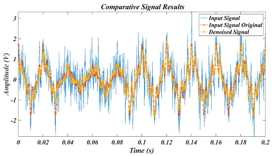
Figure 30. Comparative waveforms of Case 7 of L5 under SNR = 1 dB.

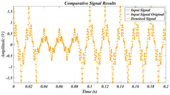
Figure 31. Comparative waveforms of Case 7 of L5 under SNR = 50 dB.

The performance results, detailed in Table 24, illustrate a clear trend: as input SNR increases, denoising accuracy improves. In conclusion, the method delivers measurable gains, including a minimum of 5.5% SNR improvement as shown in Table 24, and correlation values close to 100% for a wide SNR range. The alignment of reconstructed signals with the originals, as depicted in Figure 30 and Figure 31, affirms the technique’s reliability and application potential.

Table 24. Metric results for the synthetic signal in Case 7 of L5.

${\mathit{S}\mathit{N}\mathit{R}}_{\mathit{n}\mathit{o}\mathit{i}\mathit{s}\mathit{y}}$	${\mathit{S}\mathit{N}\mathit{R}}_{\mathit{d}\mathit{e}\mathit{n}\mathit{o}\mathit{i}\mathit{s}\mathit{e}\mathit{d}}$	${\mathit{S}\mathit{N}\mathit{R}}_{\mathit{i}\mathit{m}\mathit{p}}$ (%)	${\mathit{R}\mathit{M}\mathit{S}\mathit{E}}_{\mathit{n}\mathit{o}\mathit{i}\mathit{s}\mathit{y}}$	${\mathit{R}\mathit{M}\mathit{S}\mathit{E}}_{\mathit{d}\mathit{e}\mathit{n}\mathit{o}\mathit{i}\mathit{s}\mathit{e}\mathit{d}}$	${\mathit{R}\mathit{M}\mathit{S}\mathit{E}}_{\mathit{i}\mathit{m}\mathit{p}}$ (%)	${\mathit{M}\mathit{S}\mathit{E}}_{\mathit{n}\mathit{o}\mathit{i}\mathit{s}\mathit{y}}$	${\mathit{M}\mathit{S}\mathit{E}}_{\mathit{d}\mathit{e}\mathit{n}\mathit{o}\mathit{i}\mathit{s}\mathit{e}\mathit{d}}$	${\mathit{M}\mathit{S}\mathit{E}}_{\mathit{i}\mathit{m}\mathit{p}}$ (%)	${\mathit{C}\mathit{o}\mathit{r}\mathit{r}}_{\mathit{n}\mathit{o}\mathit{i}\mathit{s}\mathit{y}}$	${\mathit{C}\mathit{o}\mathit{r}\mathit{r}}_{\mathit{d}\mathit{e}\mathit{n}\mathit{o}\mathit{i}\mathit{s}\mathit{e}\mathit{d}}$	${\mathit{C}\mathit{o}\mathit{r}\mathit{r}}_{\mathit{i}\mathit{m}\mathit{p}}$ (%)
1	9.104	810.388	0.628	0.241	61.659	0.394	0.058	85.299	0.741	0.937	26.410
2	9.067	353.339	0.542	0.242	55.404	0.294	0.058	80.112	0.766	0.936	22.250
3	9.908	230.253	0.489	0.219	55.143	0.239	0.048	79.879	0.810	0.948	16.932
4	10.845	171.134	0.449	0.197	56.145	0.202	0.039	80.767	0.836	0.958	14.590
5	12.020	140.407	0.394	0.172	56.380	0.156	0.030	80.973	0.875	0.969	10.805
10	16.353	63.526	0.223	0.104	53.097	0.050	0.011	78.001	0.951	0.988	3.952
15	20.975	39.831	0.123	0.061	50.290	0.015	0.004	75.289	0.984	0.996	1.206
20	25.340	26.700	0.071	0.037	47.430	0.005	0.001	72.364	0.995	0.999	0.382
25	30.610	22.438	0.038	0.020	46.079	0.001	0.000	70.925	0.999	1.000	0.106
30	34.567	15.225	0.022	0.013	41.329	0.000	0.000	65.577	0.999	1.000	0.033
35	38.860	11.028	0.012	0.008	33.881	0.000	0.000	56.283	1.000	1.000	0.008
40	43.159	7.898	0.007	0.005	30.249	0.000	0.000	51.347	1.000	1.000	0.003
45	48.358	7.462	0.004	0.003	30.355	0.000	0.000	51.496	1.000	1.000	0.001
50	52.724	5.447	0.002	0.002	25.359	0.000	0.000	44.287	1.000	1.000	0.000

Key indicators, such as ${SNR}_{denoised }$ and ${Corr}_{imp}$ increase, while RMSE and MSE fall toward zero, supporting the visual observations. The top-performing models for Case 7 are listed in Table 25. Those using median and Bayes threshold rules perform best across noise levels. In contrast, wavelet type shows inconsistent effects, suggesting that visual quality is more sensitive to parameter selection than transform basis.

Table 25. Best models for each SNR level for the synthetic signal in Case 7 of L5.

SNR (dB)	Level	Wavelet Type	Threshold Rule	Denoising Method	SNR (dB)	Level	Wavelet Type	Threshold Rule	Denoising Method	SNR (dB)	Level	Wavelet Type	Threshold Rule	Denoising Method
1	5	db6	Soft	SURE	10	5	bior6.8	Soft	SURE	35	4	db6	Median	Bayes
2	5	coif4	Mean	Bayes	15	5	fk18	Soft	SURE	40	4	db8	Hard	UT
3	5	db10	Mean	Bayes	20	2	db10	Mean	Bayes	45	7	coif4	Median	Bayes
4	5	coif5	Mean	Bayes	25	2	coif5	Mean	Bayes	50	3	bior5.5	Median	Bayes
5	9	coif4	Mean	Bayes	30	4	bior5.5	Mean	Bayes	39	4	db8	Median	Bayes

4.4. Results for Experimental Data

The last signal set to be tested was the PQD signal for the experimental dataset in Table 2. There are no original signal inputs for these signals; the proposed method is performed on these signals without the original signal input and is only evaluated by the SNR metric.

The Pure signal in Case 1 is illustrated in Figure 32, which shows a high compatibility with the estimated signal without the original signal input. Another PQD signal, the sag signal in Case 2, was somewhat noisy, as shown in Figure 33. However, it exhibited high compatibility with the estimated signal on the pure side of the signal. A distinct incompatibility was observed during the sag event, unlike in Case 1.

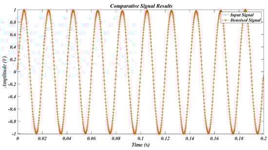
Figure 32. Comparative waveforms for Case 1 of L5.

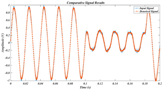
Figure 33. Comparative waveforms for Case 2 of L5.

A similar but inverse signal, that is, the swell signal in Case 3, was visible with low noise, as shown in Figure 34. Therefore, there was high compatibility with the estimated signal, as in Case 1. Case 4 for the flicker signal has some noise and fluctuation because of the inserted components leading to flicker, as shown in Figure 35. The comparative figure for this case is also consistent. Another signal with components is the harmonic signal in Case 5, as shown in Figure 36. A comparison of the noisy and denoised signals shows some inconsistency at the extreme points of the signals owing to the behavior of the harmonics.

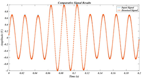
Figure 34. Comparative waveforms for Case 3 of L5.

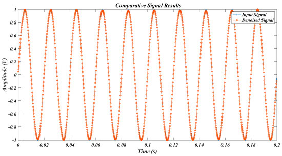
Figure 35. Comparative waveforms for Case 4 of L5.

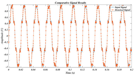
Figure 36. Comparative Waveforms for Case 5 of L5.

Case 6 was a signal with spikes, as shown in Figure 37. The proposed method provides a coherent result but with some amplitude degradation. The signal in Case 7 had sag and harmonics, as shown in Figure 38. A comparison of the noisy and denoised signals shows consistency, except for the endpoint of the sag event.

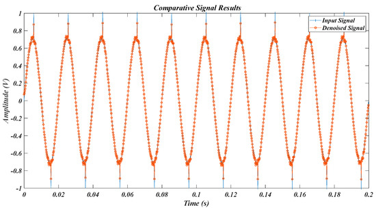
Figure 37. Comparative waveforms for Case 6 of L5.

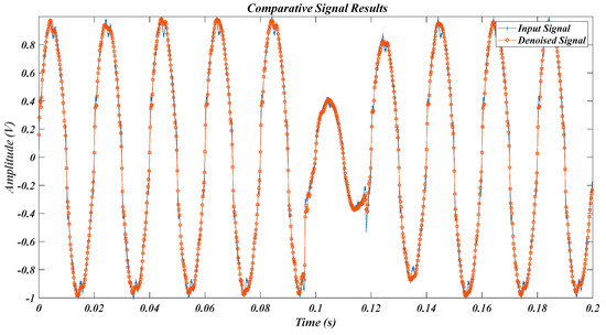
Figure 38. Comparative waveforms for Case 7 of L5.

Table 26 lists the performance metrics, such as SNR, ${SNR}_{imp}$, ${SNR}_{denoised}$, and ${SNR}_{imp}$. This is because these signals are experimental and consist of natural grid noise that changes between 16 and 40 dB per PQD signal. As can be seen from the ${SNR}_{imp}$ results in the table, the proposed model increased the SNRs of all of the PQD signals.

Table 26. SNR results for different experimental signals without the original input signal.

Case	${\mathit{S}\mathit{N}\mathit{R}}_{\mathit{n}\mathit{o}\mathit{i}\mathit{s}\mathit{y}}$ (dB)	${\mathit{S}\mathit{N}\mathit{R}}_{\mathit{d}\mathit{e}\mathit{n}\mathit{o}\mathit{i}\mathit{s}\mathit{e}\mathit{d}}$ (dB)	${\mathit{S}\mathit{N}\mathit{R}}_{\mathit{i}\mathit{m}\mathit{p}}$ (dB)	${\mathit{S}\mathit{N}\mathit{R}}_{\mathit{i}\mathit{m}\mathit{p}}$ (%)	Case	${\mathit{S}\mathit{N}\mathit{R}}_{\mathit{n}\mathit{o}\mathit{i}\mathit{s}\mathit{y}}$ (dB)	${\mathit{S}\mathit{N}\mathit{R}}_{\mathit{d}\mathit{e}\mathit{n}\mathit{o}\mathit{i}\mathit{s}\mathit{e}\mathit{d}}$ (dB)	${\mathit{S}\mathit{N}\mathit{R}}_{\mathit{i}\mathit{m}\mathit{p}}$ (dB)	${\mathit{S}\mathit{N}\mathit{R}}_{\mathit{i}\mathit{m}\mathit{p}}$ (%)
1	40.634	60.962	20.328	50.028	5	16.244	18.639	2.395	14.747
2	38.732	56.081	17.349	44.794	6	22.522	26.106	3.583	15.909
3	37.522	58.226	20.703	55.176	7	16.322	18.981	2.659	16.293
4	36.037	65.567	29.53	81.944

The experimental PQD signals are presented in Table 27. Although models consisting of “5, Soft, UniversalThreshold” are the best for most PQD signals, no models based on wavelet type assure the best performance and it changed according to the disturbance type.

Table 27. Best models for each experimental signal.

Case	Level	Wavelet Type	Threshold Rule	Denoising Method	Case	Level	Wavelet Type	Threshold Rule	Denoising Method
1	5	db9	Soft	UniversalThreshold	5	4	sym2	Soft	UniversalThreshold
2	4	db8	Soft	UniversalThreshold	6	5	fk22	Soft	UniversalThreshold
3	9	coif5	Soft	UniversalThreshold	7	5	fk22	Soft	UniversalThreshold
4	5	db9	Soft	UniversalThreshold

This study makes several significant contributions to the existing body of literature. First, it is the pioneering work that comprehensively examines both medical and experimentally obtained PQD signals. A robust and extensive denoising strategy was introduced, encompassing 4558 iterative parameter evaluations to ensure broad coverage of the solution space. The proposed methodology has demonstrated high adaptability and reliability in both reference-based and reference-free signal processing contexts. Extensive testing across a wide SNR range (1–50 dB) confirmed the algorithm’s stability, even under severely noisy conditions. Validation was carried out using both synthetically generated PQD signals and well-established benchmark datasets from prior studies [36,40,54], with detailed performance outcomes presented. Additionally, experimental analysis employing real-world PQD data confirmed the practical applicability of the proposed approach, further reinforcing its utility in real-life PQ monitoring scenarios.

In particular, the experimental evaluation demonstrates that the proposed denoising framework can be directly applied to real-world power quality monitoring systems, where accurate noise removal is essential for the reliable detection of disturbances. The system’s capacity to perform under various SNR levels and with minimal computational overhead makes it suitable for integration into embedded hardware or field-deployed measurement units. These characteristics highlight its practical relevance for utilities, smart grid monitoring devices, and industrial automation systems that demand robust signal preprocessing capabilities.

4.5. An Application with Classification

In this study, a classification-based evaluation framework was implemented to assess the effect of noise and denoising on synthetic ECG signals, specifically focusing on distinguishing between normal and abnormal waveforms. Synthetic ECG data were generated under varying SNRs, abnormality amplitudes, and anomaly durations using controlled parameters. Each generated signal was labeled as either normal or abnormal.

Twelve time-domain statistical features were extracted from each signal to form the feature vectors. These features included mean, standard deviation, skewness, kurtosis, bandpower, RMS, minimum value, maximum value, range, interquartile range, mean absolute difference, and first-lag autocorrelation coefficient.

These features were calculated separately for the clean, noisy, and denoised versions of the ECG signals.

A decision tree classifier was trained using only the clean dataset and evaluated using 10-fold cross-validation. The classifier achieved a mean accuracy of 100% on the clean dataset, indicating strong model performance under ideal signal conditions. This trained model was then applied directly to the noisy and denoised datasets to evaluate classification robustness under degraded and recovered signal conditions.

A class-specific performance analysis revealed a pronounced asymmetry in the impact of noise. While abnormal signals were still correctly classified with 100.00% accuracy in the noisy dataset, normal signals were significantly affected, with classification accuracy dropping to just 32.41%. Following the denoising process, the accuracy for normal signals markedly improved to 96.81%, while the classification accuracy for abnormal signals decreased slightly to 84.44%. These results suggest that noise has a more substantial masking effect on regular (normal) rhythms than on abnormal patterns, and that the denoising procedure is particularly effective in restoring normal signal characteristics. The classification outcomes for the clean, noisy, and denoised datasets are presented in Table 28 with detailed accuracy metrics.

Table 28. Comparative accuracy rates of the signal for classification.

Dataset	True Positives (Abnormal)	True Negatives (Normal)	False Positives	False Negatives	Accuracy (%)
Clean	100%	100%	0%	0%	100.00
Noisy	100.00%	32.41%	67.59%	0%	66.20
Denoised signal with proposed method	84.44%	96.81%	3.19%	15.56%	90.63

These results demonstrate that although the classifier trained on clean data suffers performance degradation under noise, the application of the proposed denoising strategy significantly recovers discriminative signal characteristics, particularly for normal waveforms. This validates the integration of denoising mechanisms as a crucial pre-processing step in automated ECG classification pipelines for real-world scenarios.

Moreover, this finding directly supports the use of the proposed method in practical biomedical monitoring systems, where ECG signals are often subject to motion artifacts, power-line interference, or sensor noise. By restoring the fidelity of normal signals, the framework enhances the reliability of downstream classification algorithms used in wearable healthcare devices, remote patient monitoring platforms, and real-time diagnostic tools. The lightweight computational structure also makes it suitable for embedded implementations in portable ECG units, demonstrating its applicability beyond theoretical experimentation.

4.6. Comparison with Different Hardware Platforms

The proposed method was conducted with benchmarking experiments across four different hardware setups, as shown in Table 29. These results indicate that the proposed framework can benefit substantially from parallel processing architectures. While standard desktop systems offer reasonable performance, the deployment on GPU-enabled and HPC environments, particularly those with high-core CPUs and specialized accelerators like the NVIDIA P100, can drastically reduce execution time, making the method highly suitable for real-time or large-scale denoising applications.

Table 29. Comparison of different hardware platforms.

System No	Hardware Specifications	Execution Time (s)	Description
1	Intel Core i7-10700 @ 2.90 GHz, 32 GB RAM	22.15	Desktop-class 8-core CPU; reference baseline system.
2	Intel Core i7-8750H @ 2.20 GHz, 32 GB RAM	30.85	Laptop-core CPU; lower base clock, reduced thermal performance.
3	Intel Xeon W-2223, 64 GB RAM, NVIDIA Quadro P4000 GPU	12.5	Multi-threaded Xeon + moderate GPU acceleration via Quadro P4000.
4	Truba Barbun CUDA Server: 2× Intel Xeon Gold 6148 (40 cores), 2× NVIDIA P100 GPUs, 100 Gbps InfiniBand	3.8	High-performance server; GPU-parallelized execution using P100 accelerators.

4.7. Comparison of the Other Methods with the Proposed Method

Wavelet-based denoising has long been applied in signal processing due to its ability to represent signals in both time and frequency domains. However, conventional thresholding methods are typically limited by fixed parameters and lack adaptability to signal-specific noise patterns. The proposed framework addresses this by optimizing key wavelet parameters, such as wavelet type, decomposition level, and thresholding rule, through systematic evaluation. Table 30 provides a comparative summary of classical methods versus the proposed optimization-based approach.

Table 30. Comparison of conventional wavelet denoising methods and the proposed framework.

Method	Advantages	Limitations
SURE	Adapts to signal statistics; balances noise and detail	Sensitive to noise variance; tuning required
Bayes	Probabilistic estimation of threshold	Assumes Gaussian noise; may mis-perform in structured noise
Minimax Thresholding	Statistically motivated; good for smooth signals	Rigid threshold; not flexible across noise levels
BlockJS/FDR	Improved spatial adaptivity; block-level denoising	Complex parameter selection; increased computation
Proposed Optimized Framework	Jointly optimizes wavelet parameters; adaptable to various noise types	Requires offline search or initialization; may need real-time tuning

Unlike conventional methods that rely on fixed or manually selected parameters, the proposed optimization-based framework dynamically identifies the most suitable combination of wavelet type, thresholding method, and decomposition level based on performance criteria. This adaptability enhances denoising robustness across a wide range of signal morphologies and noise characteristics. While classical methods like Bayes offer simplicity, they often underperform in high-noise or non-Gaussian conditions. In contrast, the proposed method provides greater flexibility, higher denoising accuracy, and improved generalization without prior assumptions on signal structure.

The runtime performance of a denoising method is a crucial metric for real-time or near-real-time applications, especially in domains such as power quality monitoring or biomedical signal processing, where decision latency is critical. Table 31 compares the proposed wavelet-based adaptive denoising framework with three recent alternatives from the literature in terms of their key features and average runtime performance. The proposed method achieved the fastest execution with a runtime of approximately 4.86 ms for a 0.2 s. signal segment. This efficiency stems from its automated adaptive wavelet selection mechanism that eliminates redundant decomposition levels and minimizes computational cost. In contrast, the EWT in [15] achieved denoising by incorporating entropy-based segment tracking, which improves local adaptivity but adds overheads, resulting in an average runtime of 11.2 ms. Similarly, the VMD in [18], while beneficial for component separation, exhibits higher computational demand with runtimes around 14.3 ms. The Transformer-based DL method proposed in [13] achieved high denoising accuracy at the expense of increased complexity and GPU dependence, with an estimated runtime between 14 and 20 ms, which may not be suitable for embedded applications.

Table 31. Comparison with conventional methods.

Method	Runtime	Key Feature
EWT [15]	11.2 ms	Entropy-tracked segments for ECG denoising
VMD [18]	14.3 ms	Optimization-enhanced decomposition for ECG
Transformer DL [13]	14–20 ms	High accuracy, high complexity, GPU required
Proposed Method	4.86 ms	Fast adaptive wavelet framework

Therefore, in terms of both adaptability and computational efficiency, the proposed method offers a promising alternative, particularly for edge or mobile computing environments where resources are constrained.

The proposed method is compared with Butterworth filters in Table 32, which have long been used for denoising due to their low computational complexity and smooth frequency response. However, their performance significantly declines in the presence of non-stationary or high-intensity noise.

Table 32. Comparison between Butterworth and the proposed wavelet-based framework.

Criteria	Butterworth/IIR Filtering (with References)	Proposed Optimized Wavelet-Based Framework
Noise Suppression	Limited under high noise (SNR ≈ 3.1 dB) [55]	High robustness via adaptive thresholding
Feature Preservation	May distort the waveforms [56,57]	Maintains morphological integrity
Reconstruction Accuracy	High error (MSE ≈ 0.18) [58]	Low error (<0.001) with optimization
Computational Performance	Fast in basic form; no adaptation [55,58]	Real-time capable (~4.86 ms per signal window)

Ref. [55] observed that Butterworth filtering achieves modest SNR gains (~3.1 dB), whereas wavelet-based approaches adapt more effectively to signal characteristics. Classical filters also risk distorting clinically relevant features [56,57], which are better preserved using multi-resolution wavelet techniques. In terms of accuracy, Butterworth-based methods result in higher reconstruction errors (MSE ≈ 0.18) [58], while the proposed framework achieves superior precision with MSE values below 0.001. Although Butterworth filters are inherently fast, the proposed wavelet-based framework also meets real-time performance needs, with average processing times of 4.86 ms per signal window.

4.8. Limitations of the Proposed Method

While the proposed wavelet-based denoising framework demonstrates high adaptability and accuracy across diverse signal types, several limitations should be acknowledged to ensure transparency and guide future improvements:

• Performance degradation in extreme noise scenarios: In cases where signals are heavily corrupted by composite or structured noise (e.g., impulsive + Gaussian), the denoising performance may degrade, particularly when the selected wavelet type is not well-suited to the underlying signal morphology.
• Scalability to very large model spaces: Although the algorithm achieves fast execution (~4.86 ms/model), expanding the wavelet families, subtypes, and denoising methods significantly increases the search space. In resource-constrained or real-time environments, this could lead to latency unless additional pruning or parallelization strategies are employed.
• Dependence on predefined parameter sets: The current framework relies on manually defined wavelet families, thresholding rules, and decomposition levels. While modular, performance is still bound by the completeness and granularity of these parameter pools. If novel methods are introduced, additional calibration may be required.
• Thresholding method sensitivity: Certain denoising methods like Bayes, SURE, etc., exhibit high sensitivity to their internal thresholding rule. Minor changes in noise level or signal variance can shift the optimal settings, especially in real-time or biomedical applications.
• Domain-agnostic noise modeling: The current framework performs denoising primarily based on signal waveform analysis without incorporating domain-specific knowledge. However, distinguishing between inherent signal fluctuations and actual noise may require application-aware strategies, especially in fields like biomedical or power systems, where physiological or operational variations can mimic noise. Future work may integrate supervised or hybrid techniques to address this challenge more effectively.

The proposed study has been implemented using real biomedical images and experimental PQD data, and promising results were obtained from applications involving a wide variety of signals. Considering the high performance of PQD data, particularly in flicker and harmonic signals that cause oscillations, the proposed method can be said to be robust to signal diversity. The proposed denoising framework was constructed with modularity in mind. All wavelet types, their sub-families, denoising techniques, and thresholding rules are defined as independent parameter sets. This structure enables the seamless integration of new wavelet families (e.g., “new_wlt”) and advanced denoising algorithms, merely updating the parameter arrays and corresponding configuration matrices. No modification to the core processing or optimization routines is required, ensuring forward compatibility with evolving signal processing methodologies. Future work may explore integrating probabilistic model selection, adaptive threshold tuning, and meta-learning approaches to enhance robustness and reduce computational burden.

5. Conclusions

This study introduces a wavelet-based denoising optimization framework that systematically explores a large model space to address reference-based and reference-free noise reduction challenges in non-stationary time-series signals. The proposed method was thoroughly validated using synthetic datasets, publicly available benchmarks, and experimentally acquired signals. The empirical results indicate strong denoising performance across multiple domains, including synthetic signals, biomedical recordings (ECG and EEG), and PQD signals. The algorithm demonstrated high computational efficiency, completing the full optimization process within 22.15 s and achieving an average per-window denoising time of 4.86 ms. These performance metrics affirm the framework’s practical applicability to real-time environments, such as portable ECG monitors, grid-integrated PQ analyzers, and smart sensor systems. The framework’s adaptability to varied noise levels and signal morphologies allows it to function as a robust pre-processing layer in classification pipelines, anomaly detection systems, and embedded diagnostic tools. Moreover, its demonstrated suitability for power quality monitoring highlights its relevance for next-generation smart grid infrastructures and intelligent electrical energy systems that require real-time, high-fidelity signal denoising. Future work will focus on extending its applicability to longer-duration signal segments and 2D biomedical images, as well as improving processing time through advanced optimization algorithms and hardware acceleration. With these enhancements, the proposed approach can be integrated into next-generation systems for reliable and efficient signal denoising in dynamic real-world applications.

References

- Pasti, L.; Walczak, B.; Massart, D.L.; Reschiglian, P. Optimization of signal denoising in discrete wavelet transform. Chemom. Intell. Lab. Syst. 1999, 48, 21–34. [Google Scholar] [CrossRef]
- Sardy, S.; Tseng, P.; Bruce, A. Robust Wavelet Denoising. IEEE Trans. Signal Process. 2001, 49, 1146–1152. [Google Scholar] [CrossRef] [PubMed]
- Shao, L.; Yan, R.; Li, X.; Liu, Y. From heuristic optimization to dictionary learning: A review and comprehensive comparison of image denoising algorithms. IEEE Trans. Cybern. 2014, 44, 1001–1013. [Google Scholar] [CrossRef] [PubMed]
- Chen, P.Y.; Selesnick, I.W. Group-sparse signal denoising: Non-convex regularization, convex optimization. IEEE Trans. Signal Process. 2014, 62, 3464–3478. [Google Scholar] [CrossRef]
- Azzouz, A.; Bengherbia, B.; Wira, P.; Alaoui, N.; Souahlia, A.; Maazouz, M.; Hentabeli, H. An efficient ECG signals denoising technique based on the combination of particle swarm optimisation and wavelet transform. Heliyon 2024, 10, e26171. [Google Scholar] [CrossRef]
- Mei, Y.; Wang, Y.; Zhang, X.; Liu, S.; Wei, Q.; Dou, Z. Wavelet packet transform and improved complete ensemble empirical mode decomposition with adaptive noise based power quality disturbance detection. J. Power Electron. 2022, 22, 1334–1346. [Google Scholar] [CrossRef]
- Narmada, A.; Shukla, M.K. A novel adaptive artifacts wavelet denoising for EEG artifacts removal using deep learning with meta-heuristic approach. Multimed. Tools Appl. 2023, 82, 40403–40441. [Google Scholar] [CrossRef]
- Yue, Y.; Chen, C.; Wu, X.; Zhou, X. An effective electrocardiogram segments denoising method combined with ensemble empirical mode decomposition, empirical mode decomposition, and wavelet packet. IET Signal Process. 2023, 17, e12232. [Google Scholar] [CrossRef]
- Fu, L.; Zhu, T.; Pan, G.; Chen, S.; Zhong, Q.; Wei, Y. Power quality disturbance recognition using VMD-based feature extraction and heuristic feature selection. Appl. Sci. 2019, 9, 4901. [Google Scholar] [CrossRef]
- Chen, M.; Li, Y.; Zhang, X.; Gao, J.; Sun, Y.; Shi, W.; Wei, S. Multiscale convolution and attention based denoising autoencoder for motion artifact removal in ECG signals. In Proceedings of the 7th International Conference on Image and Graphics Processing (ICIGP), Beijing, China, 19–21 January 2024; pp. 442–448. [Google Scholar]
- Chen, M.; Li, Y.; Zhang, L.; Liu, L.; Han, B.; Shi, W.; Wei, S. Elimination of random mixed noise in ECG using convolutional denoising autoencoder with transformer encoder. IEEE J. Biomed. Health Inform. 2024, 28, 1993–2004. [Google Scholar] [CrossRef]
- Khodayar, M.; Regan, J. Deep neural networks in power systems: A review. Energies 2023, 16, 4773. [Google Scholar] [CrossRef]
- Tao, Y.; Xu, B.; Zhang, Y. Refined self-attention transformer model for ECG-based arrhythmia detection. IEEE Trans. Instrum. Meas. 2024, 73, 4007314. [Google Scholar] [CrossRef]
- Ramana, P.V.; Reddy, G.J.; Krishna, V.S.; Reddy, Y.Y.; Reddy, V.V. A hybrid signal denoising approach using wavelet decomposition and neural network-based thresholding. In Proceedings of the 5th International Conference on Trends in Material Science and Inventive Materials (ICTMIM), Kanyakumari, India, 7–9 April 2025; pp. 1400–1404. [Google Scholar] [CrossRef]
- Elouaham, S.; Dliou, A.; Jenkal, W.; Louzazni, M.; Zougagh, H.; Dlimi, S.; Tani, A. Empirical wavelet transform based ECG signal filtering method. J. Electr. Comput. Eng. 2024, 2024, 9050909. [Google Scholar] [CrossRef]
- Nayak, A.B.; Shah, A.; Maheshwari, S.; Anand, V.; Chakraborty, S.; Kumar, T.S. An empirical wavelet transform-based approach for motion artifact removal in electroencephalogram signals. Decis. Anal. J. 2024, 10, 100420. [Google Scholar] [CrossRef]
- Xu, Y.; Zhang, K.; Ma, C.; Li, X.; Zhang, J. An improved empirical wavelet transform and its applications in rolling bearing fault diagnosis. Appl. Sci. 2018, 8, 2352. [Google Scholar] [CrossRef]
- Singh, P.; Pradhan, G. Variational mode decomposition based ECG denoising using non-local means and wavelet domain filtering. Australas. Phys. Eng. Sci. Med. 2018, 41, 891–904. [Google Scholar] [CrossRef]
- Edder, A.; Ben-Bouazza, F.E.; Tafala, I.; Manchadi, O.; Jioudi, B. Self attention-driven ECG denoising: A transformer-based approach for robust cardiac signal enhancement. Signals 2025, 6, 26. [Google Scholar] [CrossRef]
- Mishra, A.; Dharahas, G.; Gite, S.; Kotecha, K.; Koundal, D.; Zaguia, A.; Kaur, M.; Lee, H.-N. ECG data analysis with denoising approach and customized CNNs. Sensors 2022, 22, 1928. [Google Scholar] [CrossRef]
- Mohagheghian, F.; Han, D.; Ghetia, O.; Peitzsch, A.; Nishita, N.; Nejad, M.P.S.; Ding, E.Y.; Noorishirazi, K.; Hamel, A.; Otabil, E.M.; et al. Noise reduction in photoplethysmography signals using a convolutional denoising autoencoder with unconventional training scheme. IEEE Trans. Biomed. Eng. 2023, 71, 456–466. [Google Scholar] [CrossRef]
- Caicedo, J.E.; Agudelo-Martínez, D.; Rivas-Trujillo, E.; Meyer, J. A systematic review of real-time detection and classification of power quality disturbances. Prot. Control Mod. Power Syst. 2023, 8, 3. [Google Scholar] [CrossRef]
- Chen, M.; Cheng, Q.; Feng, X.; Zhao, K.; Zhou, Y.; Xing, B.; Tang, S.; Wang, R.; Duan, J.; Wang, J.; et al. Optimized variational mode decomposition algorithm based on adaptive thresholding method and improved whale optimization algorithm for denoising magnetocardiography signal. Biomed. Signal Process. Control 2024, 88, 105681. [Google Scholar] [CrossRef]
- Roy, A.; Satija, U. A novel deep metric learning based state-stable and noise-aware biometric authentication framework using seismocardiogram signals. IEEE Trans. Biom. Behav. Ident. Sci. 2024, 7, 246–255. [Google Scholar] [CrossRef]
- Qin, A.; Mao, H.; Sun, K.; Huang, Z.; Li, X. Cross-domain fault diagnosis based on improved multi-scale fuzzy measure entropy and enhanced joint distribution adaptation. IEEE Sens. J. 2022, 22, 9649–9664. [Google Scholar] [CrossRef]
- Rezazadeh, N.; Perfetto, D.; Polverino, A.; De Luca, A.; Lamanna, G. Guided wave-driven machine learning for damage classification with limited dataset in aluminum panel. Struct. Health Monit. 2024. [Google Scholar] [CrossRef]
- Ding, Y.; Selesnick, I.W. Artifact-Free Wavelet Denoising: Non-convex Sparse Regularization, Convex Optimization. IEEE Signal Process. Lett. 2015, 22, 1364–1368. [Google Scholar] [CrossRef]
- Liu, F.; Zhang, Y.; Yildirim, T.; Zhang, J. Signal denoising optimization based on a Hilbert-Huang transform-triple adaptable wavelet packet transform algorithm. Europhys. Lett. 2018, 124, 54002. [Google Scholar] [CrossRef]
- Chatterjee, S.; Thakur, R.S.; Yadav, R.N.; Gupta, L.; Raghuvanshi, D.K. Review of noise removal techniques in ECG signals. Inst. Eng. Technol. 2020, 14, 569–590. [Google Scholar] [CrossRef]
- Zhang, D.; Wang, S.; Li, F.; Tian, S.; Wang, J.; Ding, X.; Gong, R.; Sangaiah, A.K. An Efficient ECG Denoising Method Based on Empirical Mode Decomposition, Sample Entropy, and Improved Threshold Function. Wirel. Commun. Mob. Comput. 2020, 2020, 8811962. [Google Scholar] [CrossRef]
- Wang, G.; Yang, L.; Liu, M.; Yuan, X.; Xiong, P.; Lin, F.; Liu, X. ECG signal denoising based on deep factor analysis. Biomed. Signal Process Control 2020, 57, 101824. [Google Scholar] [CrossRef]
- Ghosh, S.K.; Tripathy, R.K.; Ponnalagu, R.N. Evaluation of Performance Metrics and Denoising of PCG Signal using Wavelet Based Decomposition. In Proceedings of the 2020 IEEE 17th India Council International Conference (INDICON), New Delhi, India, 11–13 December 2020; Institute of Electrical and Electronics Engineers Inc.: New York, NY, USA, 2020. [Google Scholar] [CrossRef]
- Sun, Z.; Xi, X.; Yuan, C.; Yang, Y.; Hua, X. Surface electromyography signal denoising via EEMD and improved wavelet thresholds. Math. Biosci. Eng. 2020, 17, 6945–6962. [Google Scholar] [CrossRef]
- Baldazzi, G.; Solinas, G.; Del Valle, J.; Barbaro, M.; Micera, S.; Raffo, L.; Pani, D. Systematic analysis of wavelet denoising methods for neural signal processing. J. Neural Eng. 2020, 17, 066016. [Google Scholar] [CrossRef]
- Fan, G.; Li, J.; Hao, H. Vibration signal denoising for structural health monitoring by residual convolutional neural networks. Measurement 2020, 157, 107651. [Google Scholar] [CrossRef]
- Sha, D.; Liang, W.; Wu, L. A novel noise reduction method for natural gas pipeline defect detection signals. J. Nat. Gas. Sci. Eng. 2021, 96, 104335. [Google Scholar] [CrossRef]
- Feng, G.; Wei, H.; Qi, T.; Pei, X.; Wang, H. A transient electromagnetic signal denoising method based on an improved variational mode decomposition algorithm. Measurement 2021, 184, 109815. [Google Scholar] [CrossRef]
- Wang, J.; Li, J.; Yan, S.; Shi, W.; Yang, X.; Guo, Y.; Gulliver, T.A. A Novel Underwater Acoustic Signal Denoising Algorithm for Gaussian/Non-Gaussian Impulsive Noise. IEEE Trans. Veh. Technol. 2021, 70, 429–445. [Google Scholar] [CrossRef]
- Prashar, N.; Sood, M.; Jain, S. Design and implementation of a robust noise removal system in ECG signals using dual-tree complex wavelet transform. Biomed. Signal Process. Control 2021, 63, 102212. [Google Scholar] [CrossRef]
- Kaur, C.; Bisht, A.; Singh, P.; Joshi, G. EEG Signal denoising using hybrid approach of Variational Mode Decomposition and wavelets for depression. Biomed. Signal Process. Control 2021, 65, 102337. [Google Scholar] [CrossRef]
- Zhao, Z.; Wu, Z.; Zheng, Y.; Ma, P. Recurrent neural networks for atmospheric noise removal from InSAR time series with missing values. ISPRS J. Photogramm. Remote Sens. 2021, 180, 227–237. [Google Scholar] [CrossRef]
- Shi, F. A review of noise removal techniques in ECG signals. In Proceedings of the 2022 IEEE Conference on Telecommunications, Optics and Computer Science (TOCS), Dalian, China, 11–12 December 2022; Institute of Electrical and Electronics Engineers (IEEE): New York, NY, USA, 2023; pp. 237–240. [Google Scholar] [CrossRef]
- Wang, X.; Chen, B.; Zeng, M.; Wang, Y.; Liu, H.; Liu, R.; Tian, L.; Lu, X. An ECG Signal Denoising Method Using Conditional Generative Adversarial Net. IEEE J. Biomed. Health Inf. 2022, 26, 2929–2940. [Google Scholar] [CrossRef]
- Madan, P.; Singh, V.; Singh, D.P.; Diwakar, M.; Kishor, A. Denoising of ECG signals using weighted stationary wavelet total variation. Biomed. Signal Process. Control 2022, 73, 103478. [Google Scholar] [CrossRef]
- Li, C.; Wu, Y.; Lin, H.; Li, J.; Zhang, F.; Yang, Y. ECG Denoising Method Based on an Improved VMD Algorithm. IEEE Sens. J. 2022, 22, 22725–22733. [Google Scholar] [CrossRef]
- Zhu, M.L.; Zhao, L.L.; Xiao, L. Image Denoising Based on GAN with Optimization Algorithm. Electronics 2022, 11, 2445. [Google Scholar] [CrossRef]
- Jia, N.; Cheng, Y.; Liu, Y.; Tian, Y. Intelligent Fault Diagnosis of Rotating Machines Based on Wavelet Time-Frequency Diagram and Optimized Stacked Denoising Auto-Encoder. IEEE Sens. J. 2022, 22, 17139–17150. [Google Scholar] [CrossRef]
- Yue, G.D.; Xu, Z.; Wang, L.D.; Liu, C.; Zhou, W.J. Vibration analysis for slab track at different train speeds using Bayes wavelet denoising. Proc. Inst. Mech. Eng. F J. Rail Rapid Transit 2017, 231, 892–901. [Google Scholar] [CrossRef]
- Katicha, S.W.; Loulizi, A.; John; Khoury, E.; Asce, M.; Flintsch, G.W. Adaptive False Discovery Rate for Wavelet Denoising of Pavement Continuous Deflection Measurements. J. Comput. Civ. Eng. 2016, 31, 04016049. [Google Scholar] [CrossRef]
- Karim, S.A.A.; Ismail, M.T.; Hasan, M.K.; Sulaiman, J.; Sakidin, H. Denoising using new thresholding method. In AIP Conference Proceedings; American Institute of Physics Inc.: College Park, MD, USA, 2016. [Google Scholar] [CrossRef]
- Dai, T.; Li, Y. Efficient dual domain image denoising via SURE-based optimization. Int. J. Mach. Learn. Cybern. 2023, 14, 4417–4430. [Google Scholar] [CrossRef]
- Nguyen, H.V.; Ulfarsson, M.O.; Sveinsson, J.R. Hyperspectral Image Denoising Using SURE-Based Unsupervised Convolutional Neural Networks. IEEE Trans. Geosci. Remote Sens. 2021, 59, 3369–3382. [Google Scholar] [CrossRef]
- Li, J.; Tong, Y.; Guan, L.; Wu, S.; Li, D. A UV-visible absorption spectrum denoising method based on EEMD and an improved universal threshold filter. RSC Adv. 2018, 8, 8558–8568. [Google Scholar] [CrossRef]
- Moody, G.B.; Mark, R.G. The impact of the MIT-BIH Arrhythmia Database. IEEE Eng. Med. Biol. Mag. 2001, 20, 45–50. [Google Scholar] [CrossRef]
- Sørensen, J.S.; Johannesen, L.; Grove, U.S.L.; Lundhus, K.; Couderc, J.P.; Graff, C. A Comparison of IIR and Wavelet Filtering for Noise Reduction of the ECG. Comput. Cardiol. 2010, 37, 489–492. [Google Scholar]
- Yusuf, S.D.; Maduakolam, F.C.; Umar, I.; Loko, Z.A. Analysis of Butterworth Filter for Electrocardiogram De-Noising Using Daubechies Wavelets. SSRG Int. J. Electron. Commun. Eng. 2020, 7, 8–13. [Google Scholar] [CrossRef]
- Jia, Y.; Pei, H.; Liang, J.; Zhou, Y.; Yang, Y.; Cui, Y.; Xiang, M. Preprocessing and Denoising Techniques for Electrocardiography and Magnetocardiography: A Review. Bioengineering 2024, 11, 1109. [Google Scholar] [CrossRef]
- Yadav, O.P.; Ray, S. Analysis of Butterworth and Chebyshev Filters for ECG Denoising Using Wavelets. IOSR J. Electron. Commun. Eng. 2013, 6, 37–44. [Google Scholar] [CrossRef]
Disclaimer/Publisher’s Note: The statements, opinions and data contained in all publications are solely those of the individual author(s) and contributor(s) and not of MDPI and/or the editor(s). MDPI and/or the editor(s) disclaim responsibility for any injury to people or property resulting from any ideas, methods, instructions or products referred to in the content. |
© 2025 by the author. Licensee MDPI, Basel, Switzerland. This article is an open access article distributed under the terms and conditions of the Creative Commons Attribution (CC BY) license (https://creativecommons.org/licenses/by/4.0/).