Abstract
The synchronous reference frame phase-locked loop (SRF-PLL) is widely employed for grid synchronization in wind farms. However, it may exhibit oscillations under voltage sags or improper parameter settings. These oscillations may compromise the secure integration of large-scale wind power. Therefore, mitigating the oscillations of the SRF-PLL is crucial for ensuring stable and reliable operation. To this end, this paper investigates the underlying oscillation mechanism of the SRF-PLL from local and global perspectives. By taking into account the grid voltage and control parameters, it is revealed that oscillations of the SRF-PLL can be triggered by grid voltage sags and/or the improper control parameters. More specifically, from the local perspective, the SRF-PLL exhibits distinct qualitative behaviors around its stable equilibrium points under different grid voltage amplitudes. As a result, when grid voltage sags occur, the SRF-PLL may exhibit multiple oscillation modes and experience a prolonged transient response. Furthermore, from the global viewpoint, the large-signal analysis reveals that the SRF-PLL has infinitely many asymmetrical convergence regions. However, the sizes of these asymmetrical convergence regions shrink significantly under low grid voltage amplitude and/or small control parameters. In this case, even if the parameters in the small-signal model of the SRF-PLL are well-designed, a small disturbance can shift the operating point into other regions, resulting in undesirable oscillations and a sluggish dynamic response. The validity of the theoretical analysis is further supported by experimental verification.
1. Introduction
For grid-connected applications, synchronization is commonly required. Thus, a variety of phase-locked loop-based grid synchronization methods have been proposed in the literature [1,2], e.g., the second-order generalized integrator-based phase-locked loops (SOGI-PLL) [3], moving average filter based phase-locked loops (MAF-PLL) [4], and adaptive observer PLLs [5]. Among them, the synchronous reference frame PLL (SRF-PLL) remains the most prevalently adopted due to its simplicity and effectiveness [6,7,8,9]. In three-phase power systems, the SRF-PLL is employed to extract the phase angle, frequency, and voltage amplitude of the grid, and it plays a vital role in the control and monitoring of grid-connected converters in wind power systems.
With the rapid development of wind power generation, stability issues arising from the interaction between wind power systems and the grid have attracted increasing attention [10]. In this context, many recent studies have focused on improving power quality and synchronization, including advanced control and artificial intelligence (AI)-based control strategies [11,12,13,14]. In particular, synchronization is of critical importance, as the interaction between the SRF-PLL and grid stability has been widely explored in previous studies [15,16,17], and it has been shown that the SRF-PLL exerts a significant impact on the stability of AC grids. Meanwhile, the performance of SRF-PLL is strongly affected by the voltage conditions at the point of common coupling (PCC). To address these challenges, many enhanced PLL variants have been proposed for improved synchronization robustness and power quality under weak grids, such as Adaptive SRF-PLL [18], Extended State Observer Based PLL (ESO-PLL) [19], Dual Second-Order Generalized Integrator PLL (DSOGI-PLL) [20], and Enhanced PLL (EPLL) [21]. Each of these methods has its own advantages: Adaptive SRF-PLL dynamically tunes its parameters to accommodate different grid strengths; ESO-PLL enhances robustness against harmonics and disturbances by compensating unmodeled dynamics; DSOGI-PLL achieves accurate phase estimation under unbalanced and harmonic-distorted voltages; and EPLL provides a faster dynamic response and improved noise rejection. These improvements primarily target weak-grid and distorted-voltage conditions, while comparative studies under severe voltage sags are still limited in the literature. Although these advanced structures introduce additional adaptability or filtering components, they are generally built upon the conventional SRF-PLL framework. Therefore, a comprehensive evaluation of the SRF-PLL’s dynamic performance under different grid conditions remains essential, as it not only informs the design of wind turbine controllers but also provides valuable insights for the development of advanced PLL algorithms.
To this end, the SRF-PLL is modeled by a simplified small-signal model based on which the performance of the nonlinear SRF-PLL can be easily analyzed in the linear framework (linear analysis methods) [22]. However, the small-signal model can not accurately reflect its dynamics. The small-signal model-based methods are effective under the specific assumption that the estimated frequency closely matches the actual grid frequency . However, when this assumption does not hold, ignoring their differences may obscure important dynamic characteristics of the system [23,24]. In fact, previous studies have indicated that large frequency deviations can lead to sluggish dynamic behavior in the SRF-PLL [22].
Small-signal model methods focus on local behavior, whereas the large-signal model-based analysis provides a direct insight into the overall performance of the SRF-PLL. In [25], a large-signal model was established, based on which the global stability analysis of the SRF-PLL was conducted. Using the phase-portrait approach, it is shown in [25] that the SRF-PLL possesses infinitely many stable equilibrium points and corresponding convergence regions. However, the study in [25] does not explicitly address the underlying oscillation mechanisms under voltage sags and improper control parameters, which are common and critical in weak grid scenarios. In practical systems, voltage sags caused by grid faults are common and pose significant challenges to maintaining reliable synchronization and satisfactory control performance, as required by grid codes. Therefore, it is desirable to disclose the oscillation mechanism with respect to grid voltage and control parameters, since such insights can provide valuable guidance for parameter tuning and robust controller design in wind turbine applications.
Building on the above, this study aims to fill this gap by offering new insights into how grid voltage amplitudes and parameter settings give rise to undesirable oscillations in the SRF-PLL. Firstly, the nonlinear large-signal model for the SRF-PLL is derived, and subsequently, the phase-portrait method is adopted to investigate how the SRF-PLL behaves under different grid voltage amplitudes and control parameters. Based on the in-depth theoretical analysis, this study reveals that the performance of the SRF-PLL is highly sensitive to grid voltage amplitude and control parameter settings. In particular, undesirable oscillations may arise under voltage sags and/or improper control parameter, posing a serious threat to system stability. The contributions of this paper are summarized as follows:
- SRF-PLL oscillation analysis around stable equilibrium points. This paper demonstrates that the SRF-PLL has distinct qualitative behaviors around stable equilibrium points for different grid voltage amplitudes. In the vicinity of a stable equilibrium point, the SRF-PLL under a normal grid voltage converges directly to that point without oscillations. However, when the grid voltage amplitude drops significantly, the SRF-PLL may exhibit multiple oscillations, leading to an extended transient response.
- SRF-PLL oscillation analysis from a global viewpoint.This paper reveals that the sizes of the convergence regions of SRF-PLL are influenced by the grid voltage amplitude and control parameters. When the grid voltage amplitude and/or control parameters are small, these convergence regions shrink significantly. In this case, a small disturbance, e.g., a small frequency jump, can cause the state of the SRF-PLL to move outside the original convergence region. Consequently, undesirable oscillations and a prolonged transient process may occur, even if the control parameters and have been carefully designed according to the SRF-PLL’s small-signal model.
The rest of the paper is organized as follows. Section 2 reviews the large signal model of the SRF-PLL. Section 3 investigates the relationship between grid voltage, control parameters, and the oscillation mechanism of the SRF-PLL. The experimental validation of the analysis is presented in Section 4. Section 5 concludes this paper, while Section 6 provides further discussion and outlines potential future work.
2. Large-Signal Model of the SRF-PLL
Figure 1 illustrates the structure of the SRF-PLL, which includes three main components: a phase detector (PD), a loop filter (LF), and a voltage-controlled oscillator (VCO) [22]. The ideal grid voltages in a three-phase system, denoted as , , and , can be mathematically represented as follows:
where V corresponds to the voltage magnitude, to the frequency, to the phase, and to the initial phase angle of the grid voltage. To facilitate analysis in the rotating reference frame, the Clarke-Park transformation T is applied to convert variables into quantities:
where denotes the estimated value of , and the grid voltages defined in (1) are then converted into the reference frame:
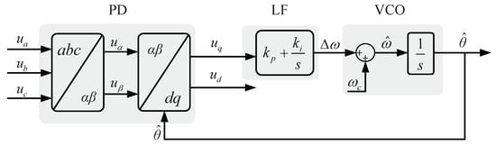
Figure 1.
Block diagram of the SRF-PLL.
Taking the as the input of the LF, its output is given by the following:
where and are the control parameters in the SRF-PLL (see Appendix A. Nomenclature for descriptions and units). The output of the LF then drives the VCO, which produces the estimated frequency and estimated phase as follows:
in which represents the nominal grid frequency and remains constant throughout the operation.
Taking the derivatives of the estimated frequency and phase defined in (6) yields the following:
To proceed with the derivation, we define the phase and frequency estimation errors as the differences between the estimated and actual values, i.e., and . Calculating the derivatives of these estimation errors leads to
Substituting the expression of from Equation (4) into the above Equation (8) yields
which provides a large-signal representation that reflects the nonlinear dynamics of the SRF-PLL. Equation (9) clearly indicates that the SRF-PLL’s performance is affected by grid voltage amplitude V and control parameters and . In the next section, the underlying oscillation mechanisms of the SRF-PLL are investigated in-depth from both local and global perspectives.
3. Oscillations Mechanism of the SRF-PLL
In this section, the undesirable oscillations of the SRF-PLL are further analyzed under different grid voltage amplitudes and control parameters. The relationships among the grid voltage amplitudes, control parameters, and oscillations of the SRF-PLL are revealed as follows.
3.1. SRF-PLL Oscillation Around Stable Equilibrium Points
From the large-signal model described in (9), its corresponding equilibrium points satisfy the following condition:
which implies that the SRF-PLL possesses an infinite number of equilibrium points located at . To facilitate analysis, we define the transformed variables and . By performing Taylor series expansion of the nonlinear system described by Equation (9) around the equilibrium points , we obtain a linearized model as follows:
where
The theoretical foundation of this linearization method can be found in [26].
Around each equilibrium points, the SRF-PLL exhibits behavior analogous to the linearized system described by (11). Clearly, when , it follows that . A straightforward calculation then shows that the corresponding linearized system of (11) is unstable. In this case, the equilibrium points are unstable due to the presence of one eigenvalue of with a positive real part and another with a negative real part. In addition, if , . In this case, the linear system of (11) is stable, and hence, the equilibrium points are stable points. This indicates that within a small neighborhood of a stable point, the SRF-PLL will converge to that stable point eventually. However, the eigenvalues of rely on the grid voltage V and control parameters and . has two complex eigenvalues:
From (12), the real part of the eigenvalues is , which represents the decay rate of the system’s dynamics. A more negative real part indicates faster attenuation of oscillations. Hence, a smaller grid voltage V or a smaller control parameter leads to slow dynamic for the SRF-PLL. In addition, the ratio between the imaginary part and real part is
which is closely related to the damping ratio, a measure of how quickly oscillations decay. When the grid voltage amplitude is small, this ratio increases, which means the damping ratio of the SRF-PLL decreases, resulting in more pronounced and sustained oscillations.
In summary, even if the control parameters and are well-designed for the normal grid voltage, a small voltage amplitude, like a grid voltage sag, may result in oscillations and slow dynamics of the SRF-PLL. To clearly illustrate the relationship between grid voltage amplitude and the oscillation characteristics of the SRF-PLL, the phase portraits corresponding to grid voltage amplitudes of 1 p.u. and p.u. are shown in Figure 2. The control parameters and are kept identical in both cases. When the amplitude of the grid voltage is the normal value (1 p.u.), the SRF-PLL settles at the stable point without oscillations. In contrast, when the voltage amplitude drops to p.u., the SRF-PLL exhibits significant oscillations according to Figure 2. It confirms the above analysis.
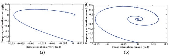
Figure 2.
Phase portraits illustrating the relationship between grid voltage amplitude and SRF-PLL oscillation. (a) Grid voltage amplitude = 1 p.u. and (b) grid voltage amplitude = p.u.
3.2. Global Oscillation Analysis for the SRF-PLL
The above analysis addresses the local stability condition. In the following, undesirable oscillations of the SRF-PLL are discussed from a global viewpoint.
Firstly, a rigorous Lyapunov analysis is performed to demonstrate that, given any initial states within a convergence region, the trajectory , for , will stay confined within this convergence region and approach its corresponding stable point asymptotically.
To simplify the analysis, we first define the intermediate variables as
Based on the defined intermediate variables, the original model in (9) is transformed into the following equivalent large-signal expression:
The nonlinear characteristics of the SRF-PLL make the Lyapunov function construction and subsequent stability analysis difficult. Therefore, the variable gradient approach is adopted to facilitate the construction of a suitable Lyapunov function. Specifically, define be a scalar function of and assume that its gradient vector with respect to the state vector can be expressed as
The derivative of along the trajectories of system (15) is given by
The variable gradient method is to determine a suitable function that serves as the gradient of a positive definite function and, at the same time, ensures that the derivative of U along the system trajectories satisfies the Lyapunov stability conditions, i.e.,
Let us consider
where denotes the scalar function, while and are constants to be determined. Note that is a scalar function. Thus,
It implies that . Submitting (19) into (18) results in
Choosing as leads to
Consequently,
The function is then obtained as
It is clear that
Thus, is the gradient of .
Clearly, choosing and implies
It means that in the region , is positive definite and its derivative
Hence, the SRF-PLL is stable within this region. Given an initial state inside the region , the system trajectory , for all , will stay within this convergence region .
In the following, it is further shown that and by applying LaSalle’s invariance theorem [26]. Define S to denote the set of all points where , i.e.,
Hence, . Let be a trajectory that remains entirely within S, i.e.,
which leads to . Consequently, the only trajectory that remains entirely within the set S corresponds to the trivial solution . By invoking the LaSalle’s invariance theorem [26], it follows that every solution starting from an initial state converges to as . This guarantees that the SRF-PLL asymptotically converges to its stable equilibrium point inside the corresponding convergence region.
The preceding analysis rigorously proves the existence and properties of convergence regions, showing that every stable equilibrium point is associated with a corresponding convergence region, and for any initial state within this convergence region, the trajectory of SRF-PLL will eventually converge to the corresponding stable point.
Importantly, the size of each convergence region is determined by the grid voltage amplitude V and the parameters and . Specifically, lower grid voltage amplitudes and/or smaller control parameters lead to reduced convergence regions. This relationship is further illustrated by the phase portraits in Figure 3, which depict the convergence region of the SRF-PLL under different control parameters and grid voltage amplitudes. It is worth noting that the boundary of the convergence region is determined by the stable manifold of the saddle points, which specifies the set of initial conditions from which the system can achieve stable locking. States outside this region will not converge to the locked equilibrium, although the overall system may still remain stable, potentially resulting in degraded dynamic performance. As shown, either decreased controller parameters , (Figure 3b), or a reduced grid voltage amplitude V (Figure 3c) result in a noticeably smaller convergence region, corroborating the theoretical analysis presented above.
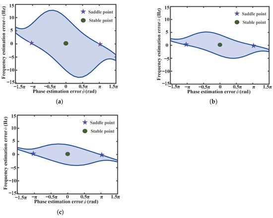
Figure 3.
Comparison of convergence regions under different control parameters , and the grid voltage amplitude V. (a) , (b) , , and (c) .
The above analysis reveals how the size of each convergence region depends on the control parameters , and the grid voltage amplitude V. Since the SRF-PLL has infinitely many such regions, the overall stability characteristic is largely governed by these parameters. In particular, when the grid voltage amplitude or the control parameters are small, the corresponding convergence regions shrink significantly. This reduction in region size decreases the system’s robustness; as a result, even minor disturbances can cause the state of the SRF-PLL to move out of its original convergence region and enter another region. Consequently, the system settles at a new stable equilibrium point that is far from the original one, resulting in significant oscillations and a prolonged transient response.
To illustrate this phenomenon vividly, Figure 4 presents a case with grid voltage amplitude p.u., and control parameters are , , representing a condition of sagged grid voltage and moderate control parameters. The control parameters of the SRF-PLL were selected based on its small-signal model [2]. Following widely used design practice [2,22], the parameters were tuned to achieve a damping ratio of about 0.707. This ensures a suitable compromise between dynamic response and robustness against disturbances. It is worth noting that the focus of this paper is on investigating how parameter variations influence the oscillation behavior and dynamic performance of the SRF-PLL rather than on proposing optimal design rules. When subjected to a Hz frequency jump, the reduced size of the convergence region causes the state of SRF-PLL to jump into Region III. As shown by the red line, this transition triggers significant oscillations, further confirming the theoretical analysis above.
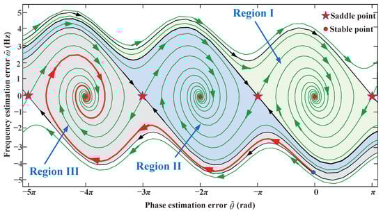
Figure 4.
Phase portraits illustrating the oscillation of SRF-PLL when grid frequency experiences a change of Hz.
4. Experimental Results
This section presents the experimental validation of the preceding analysis. The power stage hardware consists of a three-phase two-level voltage source converter built with MOSFETs. The converter is controlled by a TI TMS320F28335 digital signal processor (DSP) platform, which executes the entire SRF-PLL control algorithm and implements pulse width modulation at a switching frequency of 10 kHz. All experiments were conducted under normal laboratory conditions. The grid simulator used was the STR3060A, which is capable of generating frequency jumps and simulating various grid voltage disturbances.
4.1. Local Oscillations
In this subscetion, the SRF-PLL is tested under a 1 Hz frequency jump to verify the oscillation around stable equilibrium points. Firstly, the relationship between the grid voltage amplitude and the SRF-PLL oscillations is examined through Cases A to C. Table 1 shows the experimental parameters and the compared experimental results of these cases. Figure 5 present the phase portrait comparisons and experimental results for when the voltage amplitude p.u., p.u., and p.u., respectively. From Figure 5, it is observed that the small voltage amplitude may cause significant oscillations and a long transient process in the SRF-PLL, validating the theoretical analysis in Section 3.

Table 1.
Experimental parameters and key performance indicators for Cases A–C.
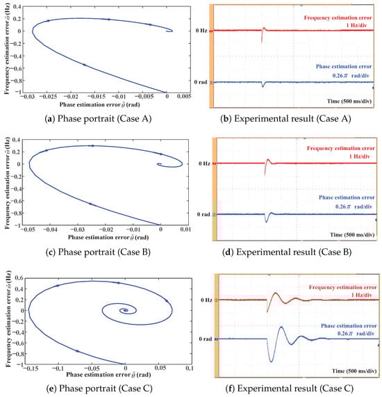
Figure 5.
Phase portraits and corresponding experimental results of the SRF-PLL under Cases A–C, demonstrating the effect of grid voltage amplitude on SRF-PLL’s local oscillations.
Furthermore, under a 1 Hz frequency jump, the relationship between the control parameters and the SRF-PLL oscillations is investigated through Cases D to F. Table 2 summarizes the experimental conditions and corresponding results for each case, while Figure 6 presents both the phase portraits and experimental waveforms. It can be observed that the small control parameters may lead to prolonged transient responses of the SRF-PLL. This observation supports the theoretical analysis presented in Section 3.
Table 2.
Experimental parameters and key performance indicators for Cases D–F.
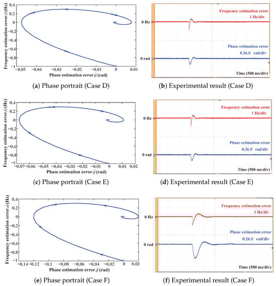
Figure 6.
Phase portraits and corresponding experimental results of the SRF-PLL under Cases D–F, illustrating the influence of control parameters on SRF-PLL’s local oscillations.
4.2. Global Oscillations
The above discussion validates the SRF-PLL’s oscillation behavior around stable equilibrium points. In this subsection, the SRF-PLL is subjected to a Hz frequency jump to verify the oscillation characteristics of the SRF-PLL from a global viewpoint. Specifically, Cases G–I investigate the influence of the grid voltage amplitude on the SRF-PLL’s global behavior. Table 3 summarizes the experimental parameters and the corresponding experimental results. Figure 7 presents the phase portraits and the experimental results of the SRF-PLL in Cases G–I. Among them, Case I features the smallest voltage amplitude, which leads to the smallest convergence region. To quantify this effect, we experimentally determined the maximum frequency jump that keeps the state within the convergence region of the equilibrium point . Specifically, this maximum tolerable frequency jump is 15.9 Hz at 1.0 p.u., decreases to 10.0 Hz at 0.5 p.u., and further drops to 3.7 Hz at 0.1 p.u. As a result, under the Hz frequency jump, the state of the SRF-PLL moves out of the original region (Region I). Consequently, the SRF-PLL in Case I experiences significant oscillations and a slow transient response, thereby confirming the theoretical analysis from a global viewpoint in Section 3.
Table 3.
Experimental parameters and key performance indicators for cases G–I.
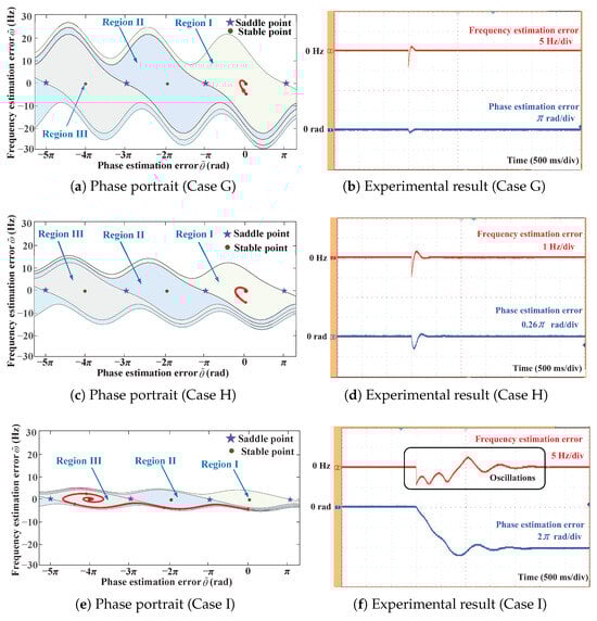
Figure 7.
Phase portraits and corresponding experimental results of the SRF-PLL under Cases G–I, demonstrating the effect of grid voltage amplitude on SRF-PLL’s global oscillations.
Furthermore, the influence of control parameters on the oscillation behavior of the SRF-PLL is investigated in Cases J–L. Table 4 presents the experimental parameters and the comparison of the experimental results across these cases. Figure 8 illustrates the phase portraits and experimental results of the SRF-PLL. Among the three cases, Case L adopts the smallest control parameters, resulting in the smallest convergence region. To quantify this effect, we also conducted experiments to identify the largest frequency jump the system can tolerate without leaving the convergence region of the equilibrium point . Specifically, this maximum tolerable frequency jump is 10 Hz for Case J, decreases to 7 Hz for Case K, and further drops to 4 Hz for Case L. Consequently, when subjected to a Hz frequency jump, the state of the SRF-PLL moves to Region II, which induces significant oscillations and a prolonged transient response. These results agree well with the theoretical analysis in Section 3.
Table 4.
Experimental parameters and key performance indicators for Cases J–L.
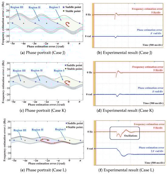
Figure 8.
Phase portraits and corresponding experimental results of the SRF-PLL under Cases J–L, illustrating the influence of control parameters on SRF-PLL’s global oscillations.
5. Conclusions
This paper investigated the underlying oscillation mechanism of the SRF-PLL. Building upon the established large-signal model, the dynamic behavior of the SRF-PLL was analyzed in-depth from both local and global perspectives, leading to the following key findings:
- (1)
- The SRF-PLL exhibits distinct dynamic behaviors around its stable equilibrium points under different grid voltage amplitudes. Consequently, during grid voltage sags, the SRF-PLL may undergo multiple oscillation modes and experience a prolonged transient response.
- (2)
- From the global viewpoint, the SRF-PLL possesses infinitely many asymmetrical convergence regions. However, their sizes shrink significantly under a low grid voltage amplitude and/or small control parameters, which increases the risk of undesirable oscillations and sluggish dynamics even when parameters are well tuned based on small-signal criteria.
These findings provide unique insights into the nonlinear dynamics of the SRF-PLL under voltage sags and improper control parameters, thereby offering valuable guidance for the design of advanced PLLs and control strategies for wind turbines.
6. Discussion and Future Work
In practical design, an important implication of this study is that the parameters initially tuned by small-signal criteria should be further checked from the perspective of a convergence region under worst-case grid disturbances specified in relevant grid codes. For instance, the Chinese standard [27] requires wind turbines to withstand a minimum voltage of 0.2 p.u. during fault-ride-through (FRT) events and remain connected for at least 625 ms. If the trajectory of the SRF-PLL exits the convergence region under such conditions, parameter adjustments are necessary until both stability and FRT duration requirements are satisfied.
Building on these findings, future research will be guided by the mechanisms revealed in this study. In particular, future research will focus on developing comprehensive parameter tuning guidelines under various grid codes, designing advanced PLL structures with improved dynamic performance and reduced sensitivity to parameter variations, as well as exploring integrated synchronization strategies to enhance robustness under weak grid conditions. These directions are expected to bridge the gap between theoretical analysis and engineering practice, ultimately supporting the reliable and large-scale integration of wind energy into power systems.
Author Contributions
Conceptualization, Z.D. and Q.S.; methodology, Z.D.; software, G.W. and S.L.; validation, G.W., S.L. and J.M.; formal analysis, G.W.; investigation, Q.S., N.L. and J.M.; resources, Z.D.; data curation, Q.S. and N.L.; writing—original draft preparation, G.W. and Z.D.; writing—review and editing, Z.D.; visualization, G.W.; supervision, Z.D.; project administration, Z.D.; funding acquisition, Z.D. All authors have read and agreed to the published version of the manuscript.
Funding
This work was supported by the National Key Research and Development Program of China under Grant 2023YFB4203200.
Data Availability Statement
The original contributions made in this study are contained within the article. Any further questions can be addressed to the corresponding author.
Conflicts of Interest
Authors Qitao Sun, Nana Lu, and Jinke Ma are employed by the Ming Yang Smart Energy Group Limited. The remaining authors declare that the research was conducted in the absence of any commercial or financial relationships that could be construed as a potential conflict of interest.
Abbreviations
| SRF-PLL | Synchronous reference frame phase-locked loop |
| SOGI-PLL | Second-order generalized integrator-based phase-locked loop |
| MAF-PLL | Moving average filter based phase-locked loop |
| ESO-PLL | Extended State Observer-Based Phase-Locked Loop |
| DSOGI-PLL | Dual Second-Order Generalized Integrator Phase-Locked Loop |
| EPLL | Enhanced Phase-Locked Loop |
| AI | Artificial intelligence |
| PCC | Point of common coupling |
| PD | Phase detector |
| LF | Loop filter |
| VCO | Voltage-controlled oscillator |
| PI | Proportional-integral |
| DSP | Digital signal processor |
| FRT | Fault ride through |
Appendix A. Nomenclature
For clarity, the main symbols used in this paper are summarized below.
| Symbol | Description | Unit |
| Three-phase grid voltage | V | |
| V | Amplitude of grid voltage | V |
| Grid voltage phase angle | rad | |
| Angular frequency | rad/s | |
| Initial phase angle of the grid voltage | rad | |
| Estimated value of grid voltage phase angle | rad | |
| Estimated value of grid angular frequency | rad/s | |
| Grid voltage in the reference frame | V | |
| Output of the LF in the SRF-PLL | rad/s | |
| Nominal grid frequency | rad/s | |
| Proportional gain of the loop filter (control parameter) | rad/(V · s) | |
| Integral gain of the loop filter (control parameter) | rad/(V · s2) | |
| Phase error: | rad | |
| Frequency error: | rad/s | |
| Auxiliary variable: | rad | |
| Auxiliary variable: | rad/s | |
| j | Imaginary unit () | – |
| Auxiliary variable: | rad | |
| Auxiliary variable: | rad/s |
References
- Golestan, S.; Guerrero, J.M.; Vasquez, J.C. Single-phase PLLs: A Review of Recent Advances. IEEE Trans. Power Electron. 2017, 32, 9013–9030. [Google Scholar] [CrossRef]
- Golestan, S.; Guerrero, J.M.; Vasquez, J.C. Three-phase PLLs: A Review of Recent Advances. IEEE Trans. Power Electron. 2017, 32, 1894–1907. [Google Scholar] [CrossRef]
- Bamigbade, A.; Khadkikar, V. Extended state-based OSG configurations for SOGI PLL with an enhanced disturbance rejection capability. IEEE Trans. Ind. Appl. 2022, 58, 7792–7804. [Google Scholar] [CrossRef]
- Golestan, S.; Ramezani, M.; Guerrero, J.M.; Freijedo, F.D.; Monfared, M. Moving average filter based phase-locked loops: Performance analysis and design guidelines. IEEE Trans. Power Electron. 2014, 29, 2750–2763. [Google Scholar] [CrossRef]
- Dai, Z.; Lin, W. Adaptive Estimation of Three-Phase Grid Voltage Parameters under Unbalanced Faults and Harmonic Disturbances. IEEE Trans. Power Electron. 2017, 32, 5613–5627. [Google Scholar] [CrossRef]
- Wang, Y.; Zhang, H.; Liu, K.; Hu, M.; Wu, Z.; Zhang, C.; Hua, W. A forward compensation method to eliminate DC phase error in SRF-PLL. IEEE Trans. Power Electron. 2022, 37, 6280–6284. [Google Scholar] [CrossRef]
- Golestan, S.; Guerrero, J.M. Conventional Synchronous Reference Frame Phase-Locked Loop is an Adaptive Complex Filter. IEEE Trans. Ind. Electron. 2015, 62, 1679–1682. [Google Scholar] [CrossRef]
- Zhang, P.; Du, W.; Wang, H. Small-signal stability of grid-connected converter system in renewable energy systems with fractional-order synchronous reference frame phase-locked loop. J. Mod. Power Syst. Clean Energy. 2025, 13, 1090–1101. [Google Scholar] [CrossRef]
- Shuai, Z.; Li, Y.; Wu, W.; Tu, C.; Luo, A.; Shen, Z.J. Divided dq Small-Signal Model: A New Perspective for the Stability Analysis of Three-Phase Grid-Tied Inverters. IEEE Trans. Ind. Electron. 2019, 66, 6493–6504. [Google Scholar] [CrossRef]
- Taul, M.G.; Wang, X.; Davari, P.; Blaabjerg, F. An overview of assessment methods for synchronization stability of grid-connected converters under severe symmetrical grid faults. IEEE Trans. Power Electron. 2019, 34, 9655–9670. [Google Scholar] [CrossRef]
- Anju, M.; Shihabudheen, K.V.; Mija, S.J. Enhancing synchronization stability: Adaptive PLL implementation using double internal loop RNN in type-3 wind power systems. Electr. Power Syst. Res. 2025, 247, 111735. [Google Scholar] [CrossRef]
- Sayeh, K.F.; Tamalouzt, S.; Ziane, D.; Bekhiti, A.; Belkhier, Y. Utilizing fuzzy logic control and neural networks based on artificial intelligence techniques to improve power quality in doubly fed induction generator-based wind turbine system. Int. J. Energy Res. 2025, 2025, 5985904. [Google Scholar] [CrossRef]
- Ramana, P.V.; Rosalina, K.M. Optimizing weak grid integrated wind energy systems using ANFIS-SRF controlled DSTATCOM. Sci. Rep. 2025, 15, 13662. [Google Scholar] [CrossRef] [PubMed]
- Ligęza, P. Basic, advanced, and sophisticated approaches to the current and forecast challenges of wind energy. Energies 2021, 14, 8147. [Google Scholar] [CrossRef]
- Wang, X.; Yao, J.; Pei, J.; Sun, P.; Zhang, H.; Liu, R. Analysis and damping control of small-signal oscillations for VSC connected to weak AC grid during LVRT. IEEE Trans. Energy Convers. 2019, 34, 1667–1676. [Google Scholar] [CrossRef]
- Nagam, S.S.; Pal, B.C.; Wu, H.; Blaabjerg, F. Synchronization stability analysis of SRF-PLL and DSOGI-PLL using port-Hamiltonian framework. IEEE Trans. Control Syst. Technol. 2025, 33, 952–962. [Google Scholar] [CrossRef]
- Hu, J.; Fu, L.; Ma, F.; Wang, G.; Liu, C.; Ma, Y. Impact of LVRT control on transient synchronizing stability of PLL-based wind turbine converter connected to high impedance AC grid. IEEE Trans. Power Syst. 2023, 38, 5445–5458. [Google Scholar] [CrossRef]
- Gonzalez-Espin, F.; Figueres, E.; Garcera, G. An Adaptive Synchronous-Reference-Frame Phase-Locked Loop for Power Quality Improvement in a Polluted Utility Grid. IEEE Trans. Ind. Electron. 2012, 59, 2718–2731. [Google Scholar] [CrossRef]
- Zhang, X.; Zhu, J.; Zheng, Z.; Liu, H.; Xue, Y.; Wan, F. Sensorless Control of PMSM Based on Fifth-Order Generalized Integral Flux Observer and Extended State Observer-Based Phase-Locked Loop. IEEE Trans. Power Electron. 2025, 40, 5080–5093. [Google Scholar] [CrossRef]
- Wang, T.; Yao, W.; Yang, H.; Li, W. Modeling and Stability Analysis of the Three-Phase Grid-Connected Inverter Under DSOGI-PLL Considering Frequency-Adaptive Feedback. IEEE J. Emerg. Sel. Top. Power Electron. 2024, 12, 4638–4651. [Google Scholar] [CrossRef]
- Golestan, S.; Matas, J.; Abusorrah, A.M.; Guerrero, J.M. More-Stable EPLL. IEEE Trans. Power Electron. 2022, 37, 1003–1011. [Google Scholar] [CrossRef]
- Teodorescu, R.; Liserre, M.; RodriGuez, P. Grid Converters for Photovoltaic and Wind Power Systems; Wiley: Hoboken, NJ, USA, 2011. [Google Scholar]
- He, X.; Geng, H.; Xi, J.; Guerrero, J.M. Resynchronization analysis and improvement of grid-connected VSCs during grid faults. IEEE J. Emerg. Sel. Top. Power Electron. 2021, 9, 438–450. [Google Scholar] [CrossRef]
- Wang, X.; Taul, M.G.; Wu, H.; Liao, Y.; Blaabjerg, F.; Harnefors, L. Grid-synchronization stability of converter-based resources—An overview. IEEE Open J. Ind. Appl. 2020, 1, 115–134. [Google Scholar] [CrossRef]
- Dai, Z.; Li, G.; Fan, M.; Huang, J.; Yang, Y.; Hang, W. Global Stability Analysis for Synchronous Reference Frame Phase-Locked Loops. IEEE Trans. Ind. Electron. 2022, 69, 10182–10191. [Google Scholar] [CrossRef]
- Khalil, H.K.; Grizzle, J. Nonlinear Systems; Prentice Hall: Upper Saddle River, NJ, USA, 2002. [Google Scholar]
- GB/T 19963.1-2021; Technical Specification for Connecting Wind Farm to Power System—Part 1: On Shore Wind Power. China Standards Press: Beijing, China, 2021.
Disclaimer/Publisher’s Note: The statements, opinions and data contained in all publications are solely those of the individual author(s) and contributor(s) and not of MDPI and/or the editor(s). MDPI and/or the editor(s) disclaim responsibility for any injury to people or property resulting from any ideas, methods, instructions or products referred to in the content. |
© 2025 by the authors. Licensee MDPI, Basel, Switzerland. This article is an open access article distributed under the terms and conditions of the Creative Commons Attribution (CC BY) license (https://creativecommons.org/licenses/by/4.0/).