Asymptotic Solution for Skin Heating by an Electromagnetic Beam at an Incident Angle

Abstract

We investigate the temperature evolution in the three-dimensional skin tissue exposed to a millimeter-wave electromagnetic beam that is not necessarily perpendicular to the skin surface. This study examines the effect of the beam’s incident angle. The incident angle influences the thermal heating in two aspects: (i) the beam spot projected onto the skin is elongated compared to the intrinsic beam spot in a perpendicular cross-section, resulting in a lower power per skin area; and (ii) inside the tissue, the beam propagates at the refracted angle relative to the depth direction. At millimeter-wavelength frequencies, the characteristic penetration depth is sub-millimeter, whereas the lateral extent of the beam spans at least several centimeters in applications. We explore the small ratio of the penetration depth to the lateral length scale in a nondimensional formulation and derive a leading-term asymptotic solution for the temperature distribution. This analysis does not rely on a small incident angle and is therefore applicable to arbitrary angles of incidence. Based on the asymptotic solution, we establish scaling laws for the three-dimensional skin temperature, the skin surface temperature, and the skin volume in which thermal nociceptors are activated.

1. Introduction

Millimeter-wave (MMW) systems operate with electromagnetic beams in the frequency range of 30–300 GHz. These systems play a significant role in both defense and civilian applications. The biological effects of MMW exposure—particularly the thermal effects on human skin—have been studied extensively. A number of these studies were compiled in a Special Issue of the Journal of Directed Energy: Refs. [1,2] reviewed the biological and physiological effects of exposure to an Active Denial System; Ref. [3] examined the pain threshold in the human thermal response modeling; Ref. [4] studied the reflex response to thermal pain; Ref. [5] investigated the behavioral effects of Active Denial System exposure when the subject is operating a motor vehicle; Ref. [6] explored the impact of exposure to an Active Denial System on reproductivity; Ref. [7] studied thermal injury caused by Active Denial System exposure; and Ref. [8] focused on technical aspects of MMW dosimetry used in exposure quantification.

A primary effect of MMW exposure is skin temperature increase heated by the absorbed electromagnetic power in the tissue. At frequencies between 30 and 300 GHz, the electromagnetic power is almost entirely absorbed within less than one millimeter of skin depth. This results in a rapid temperature rise in a thin skin layer and creates a steep temperature gradient in the depth direction. In the lateral directions along skin surface, the heating varies with the power density across the beam cross-section, which typically spans several centimeters on the skin surface. This pronounced difference in spatial scales between the depth and lateral directions renders lateral heat conduction negligible compared to conduction in the depth direction. When the incident electromagnetic beam is perpendicular to the skin surface, the separation of length scales allows for a simplified model of skin temperature: a one-dimensional partial differential equation governing heat conduction in the depth direction. Many previous theoretical studies have focused on this perpendicular beam case. The current study examines the thermal effects induced by an electromagnetic beam at an arbitrary incident angle. To our knowledge, the thermal effect of an electromagnetic beam at an arbitrary incident angle has not been studied previously.

This paper is organized as follows. Section 2 describes beam propagation both outside and within the skin, the absorption of electromagnetic power by the tissue, and the governing equation for the evolution of skin temperature. In Section 3, we derive an asymptotic solution to the governing equation. The analysis does not assume a small incident angle; rather, it is based on that the depth scale is much smaller than the length scale in lateral directions. Consequently, the asymptotic solution is valid for arbitrary incident angles. Section 4 explores the scaling behavior of the three-dimensional skin temperature, the skin surface temperature, and the activated skin volume. These scaling laws provide a foundation for comparing the effects of beams with different beam configurations. Section 5 discusses the main results obtained and Section 6 summarizes the study.

2. Governing Equation for Skin Temperature

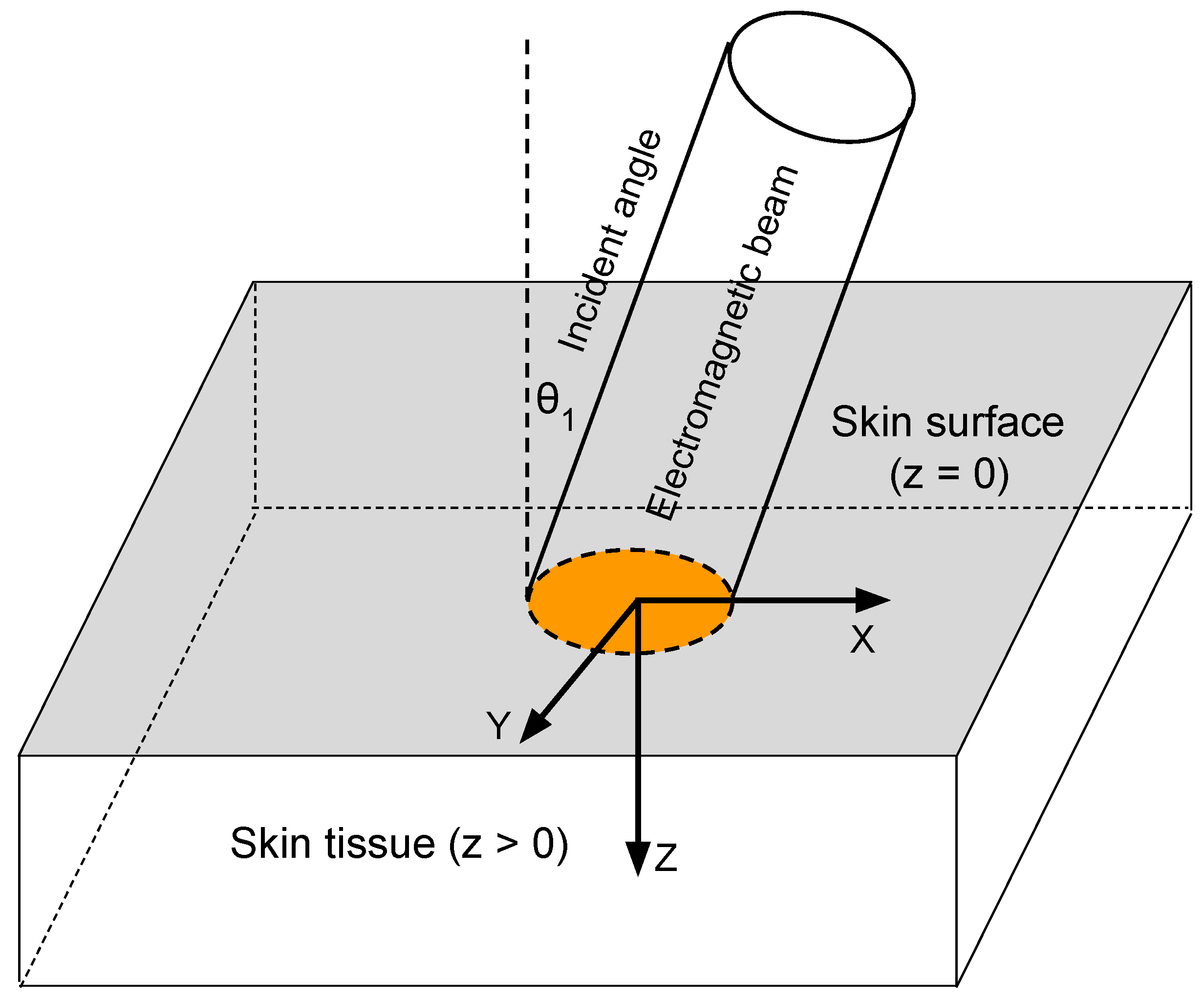
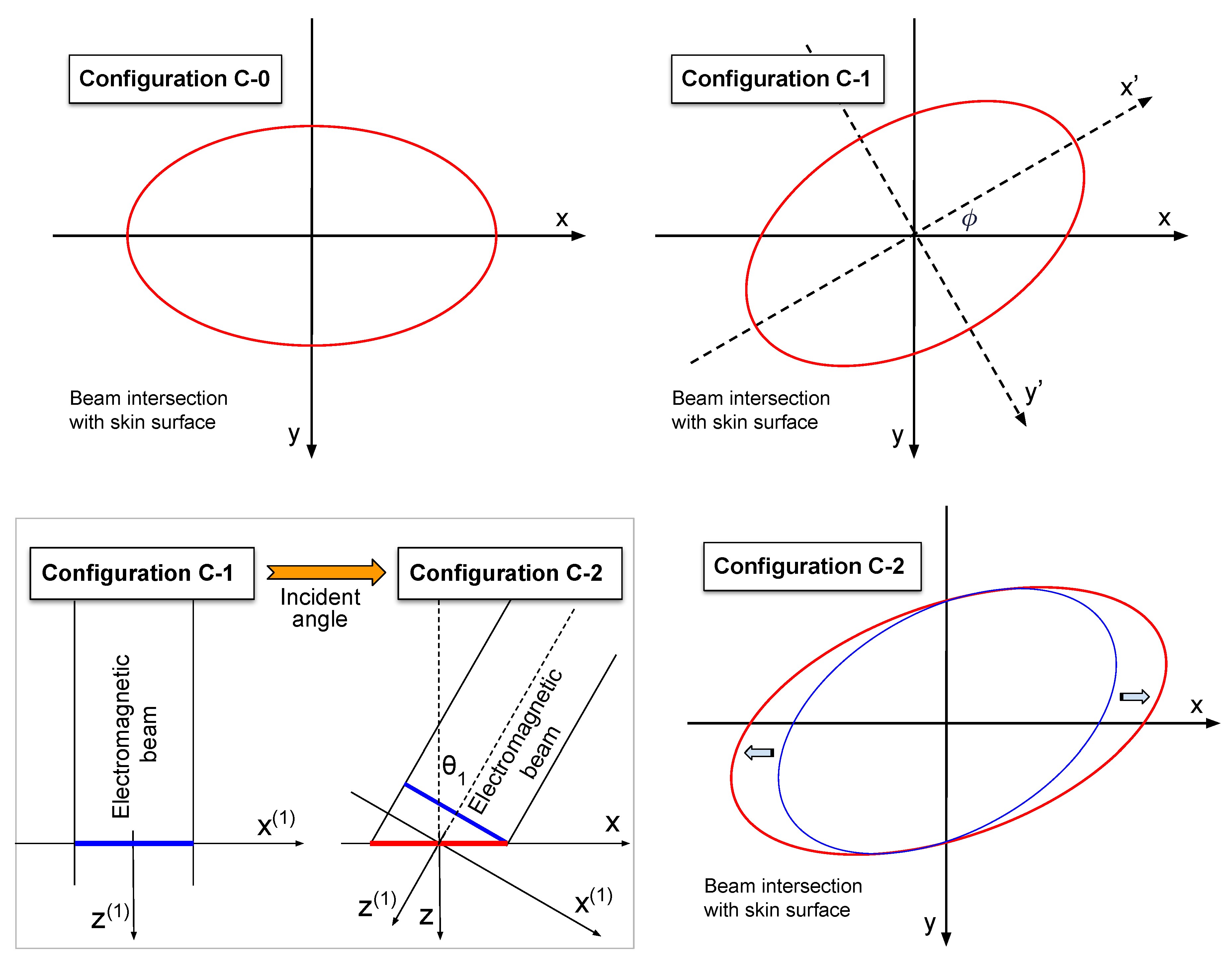
2.1. Coordinate Systems and the Incident Beam

We consider the case of a flat skin surface and establish a coordinate system similar to that used in our previous study [9]. As illustrated in Figure 1, the normal direction into the skin tissue is defined as the positive z-axis, with $z=0$ at the skin surface. The z-coordinate represents the depth into the skin. The incident beam is tilted away from the z-axis by an angle ${\theta }_1$, referred to as the incident angle. This tilt occurs within the $(x,z)$-plane, with the positive x-axis indicating the direction of the tilt. The positive y-axis is defined accordingly, completing the right-handed coordinate system.

We consider the situation where the power density over a perpendicular cross-section of the beam follows a general 2D Gaussian distribution. The general 2D Gaussian allows arbitrary aspect ratios in the perpendicular cross-section. Note that when the incident beam is tilted, the intersection of the beam with the skin surface is an angled cross-section, not a perpendicular one.

Given the 2D Gaussian power distribution, the incident beam is characterized by its configuration, which includes both the tilt of the beam axis in the $(x,z)$-plane and the rotation of the elliptical 2D Gaussian distribution about the beam axis. Let $\varphi$ be the azimuthal angle about the beam axis, between the $(x,z)$-plane and the major axis of the elliptical 2D Gaussian distribution over a perpendicular cross-section. We introduce three beam configurations:

• C-0 is the simple configuration in which the beam axis is aligned with the z-axis (i.e., zero incident angle), and the major axis of the elliptical 2D Gaussian distribution is aligned with the x-axis (i.e., zero azimuthal angle).
• C-1 is the configuration obtained by rotating C-0 about the positive z-axis (the beam axis in C-0, going into the skin) clockwise by the azimuthal angle $\varphi$.
• C-2 is the configuration obtained by rotating C-1 about the positive y-axis clockwise by the incident angle ${\theta }_1$ (tilting the beam away from the z-direction).

C-2 is the beam configuration shown in Figure 1, although the azimuthal angle $\varphi$ is not explicitly illustrated. The main objective of this paper is to study the thermal effect of a beam in configuration C-2. As described above, C-2 is obtained from C-0 through two successive rotations.

2.2. Power Density Projected onto the Skin Surface

In each of the three beam configurations introduced above, we examine the intersection of the beam with the skin surface and the power density over this intersection as a function of $(x,y)$. Here the power density refers to the power per unit area of the intersection with the skin surface, which may not necessarily be a perpendicular cross-section of the beam. In configuration C-0, the intersection with the skin surface is a perpendicular cross-section, and the power density is given by the following:

$$P_d^{\left(\mathrm{C}\text{-}0\right)}(x,y)=P_d^{\left(i\right)}exp\left({\displaystyle \frac{-1}{2}}({\displaystyle \frac{x^2}{{\sigma }_1^2}}+{\displaystyle \frac{y^2}{{\sigma }_2^2}})\right)$$

(1)

where $P_d^{\left(i\right)}$ is the power density at the beam center over a perpendicular cross-section. We refer to $P_d^{\left(i\right)}$ as the intrinsic beam power density, as it is independent of the incident angle. Over the beam intersection with the skin surface, we represent the relative distribution of the power density concisely by using its contour at the level of $(e^{-1/2}\times \mathrm{maximum})$. For the beam in configuration C-0, the $e^{-1/2}$-maximum contour is shown in the top-left panel of Figure 2. This contour is the ellipse described by ${\displaystyle \frac{x^2}{{\sigma }_1^2}}+{\displaystyle \frac{y^2}{{\sigma }_2^2}}=1$, where ${\sigma }_1$ and ${\sigma }_2$ are, respectively, the semi-major and semi-minor axes, of the perpendicular beam cross-section.

In configuration C-1, the beam intersection with the skin surface is the same perpendicular cross-section as in configuration C-0, except that it is rotated about the beam axis by an angle $\varphi$, as shown in the top-right panel of Figure 2. The rotation is clockwise about the positive z-axis (into the page). The power density and the $e^{-1/2}$-maximum contour remain unchanged in the local coordinate system $(x^{\prime },y^{\prime })$ attached to the beam. The global coordinates $(x,y)$ and the local coordinates $(x^{\prime },y^{\prime })$ are related by the following transformation:

$$\left\{\begin{array}{c}{x}^{\prime }=xcos\varphi -ysin\varphi \hfill \\ y^{\prime }=xsin\varphi +ycos\varphi \hfill \end{array}\right.$$

(2)

In coordinates $(x,y)$, the power density of configuration C-1 is

$$\begin{array}{cc}\hfill & P_d^{\left(\mathrm{C}\text{-}1\right)}(x,y)=P_d^{\left(\mathrm{C}\text{-}0\right)}(x^{\prime },y^{\prime })\hfill \\ \hfill & =P_d^{\left(i\right)}exp\left({\displaystyle \frac{-1}{2}}({\displaystyle \frac{{\left(xcos\varphi -ysin\varphi \right)}^2}{{\sigma }_1^2}}+{\displaystyle \frac{{\left(xsin\varphi +ycos\varphi \right)}^2}{{\sigma }_2^2}})\right)\hfill \end{array}$$

(3)

The rotation from configuration C-1 to C-2 is illustrated in the bottom-left panel of Figure 2. The beam intersection with the skin surface in C-1 (solid blue line) is a perpendicular cross-section, while the intersection in C-2 (solid red line) is an angled cross-section at angle ${\theta }_1$ relative to the perpendicular cross-section. These two intersections are connected by beam ray lines (lines parallel to the beam axis). A point $(x,y)$ in the intersection of C-2 is traced along a beam ray line to the point $(xcos{\theta }_1,y)$ in the intersection of C-1. An area element at point $(xcos{\theta }_1,y)$ in the intersection of C-1 is mapped by beam ray lines to an area element at point $(x,y)$ in the intersection of C-2. This mapping also magnifies the area element by a factor of $(1/cos{\theta }_1)$ as it moves from C-1 to C-2.

Over the intersection with the skin surface, we represent the relative distribution of power density using its $e^{-1/2}$-maximum contour in the $(x,y)$-plane. We refer to this $e^{-1/2}$-maximum contour simply as the beam spot, or more precisely, the beam spot projected onto the skin surface. The beam spot of C-2 (red ellipse) and the beam spot of C-1 (blue ellipse) are compared in the bottom-right panel of Figure 2. Essentially, the beam spot of C-2 is obtained by stretching the beam spot of C-1 in the x-direction by a factor of $(1/cos{\theta }_1)$. When the beam is in configuration C-2, the power density over the intersection with the skin surface can be written as

$$\begin{array}{cc}\hfill & P_d^{\left(\mathrm{C}\text{-}2\right)}(x,y)=cos{\theta }_1{P}_d^{\left(\mathrm{C}\text{-}1\right)}(xcos{\theta }_1,y)\hfill \\ \hfill & =(cos{\theta }_1{P}_d^{\left(i\right)})exp\left({\displaystyle \frac{-1}{2}}({\displaystyle \frac{{\left(xcos{\theta }_{1}cos\varphi -ysin\varphi \right)}^2}{{\sigma }_1^2}}+{\displaystyle \frac{{\left(xcos{\theta }_{1}sin\varphi +ycos\varphi \right)}^2}{{\sigma }_2^2}})\right)\hfill \\ \hfill & \equiv (cos{\theta }_1{P}_d^{\left(i\right)})exp\left({\displaystyle \frac{-1}{2}}\left(a_{11}{x}^2+a_{22}{y}^2+2a_{12}xy\right)\right)\hfill \end{array}$$

(4)

where the coefficients $a_{11}$, $a_{22}$, and $a_{12}$ are functions of $({\sigma }_1,{\sigma }_2,\varphi ,{\theta }_1)$.

$$\left\{\begin{array}{c}{\displaystyle a_{11}({\sigma }_1,{\sigma }_2,\varphi ,{\theta }_1)={cos}^2{\theta }_1\left(\frac{{cos}^2\varphi }{{\sigma }_1^2}+\frac{{sin}^2\varphi }{{\sigma }_2^2}\right)}\hfill \\ {\displaystyle a_{22}({\sigma }_1,{\sigma }_2,\varphi ,{\theta }_1)=\frac{{sin}^2\varphi }{{\sigma }_1^2}+\frac{{cos}^2\varphi }{{\sigma }_2^2}}\hfill \\ a_{12}({\sigma }_1,{\sigma }_2,\varphi ,{\theta }_1)=cos{\theta }_{1}sin\varphi cos\varphi \left({\displaystyle \frac{1}{{\sigma }_2^2}}-{\displaystyle \frac{1}{{\sigma }_1^2}}\right)\hfill \end{array}\right.$$

(5)

Equation (4) is the general form of the 2D Gaussian distribution. Let $(\xi ,\eta )$ be the rotated coordinate system in which the Gaussian distribution (4) is diagonalized. We then have

$$\begin{array}{cc}\hfill & \left\{\begin{array}{c}\xi =xcos{\varphi }_2-ysin{\varphi }_2\hfill \\ \eta =xsin{\varphi }_2+ycos{\varphi }_2\hfill \end{array}\right.\hfill \end{array}$$

(6)

$$\begin{array}{cc}\hfill & a_{11}{x}^2+a_{22}{y}^2+2a_{12}xy={\displaystyle \frac{{\xi }^2}{{\sigma }_{\xi }^2}}+{\displaystyle \frac{{\eta }^2}{{\sigma }_{\eta }^2}}\hfill \end{array}$$

(7)

where ${\varphi }_2$ is the azimuthal orientation angle of the beam spot projected onto the skin surface. ${\varphi }_2$ is the clockwise angle about the positive z-axis (into the skin) from the x-axis to the major axis. $({\sigma }_{\xi },{\sigma }_{\eta })$ are the half-major and half-minor axes of the beam spot projected onto the skin surface. The projected beam spot is completely described by geometric parameters $({\sigma }_{\xi },{\sigma }_{\eta },{\varphi }_2)$. We express $({\sigma }_{\xi },{\sigma }_{\eta },{\varphi }_2)$ in terms of $({\sigma }_{\xi },{\sigma }_{\eta },{\varphi }_2)$. Substituting (6) into (7) to express both sides as quadratic forms of $(x,y)$ and equating the corresponding coefficients on both sides, we derive a set of equations for $({\sigma }_{\xi },{\sigma }_{\eta },{\varphi }_2)$.

$$\left\{\begin{array}{c}{\displaystyle \frac{{cos}^2{\varphi }_2}{{\sigma }_{\xi }^2}+\frac{{sin}^2{\varphi }_2}{{\sigma }_{\eta }^2}=a_{11}}\hfill \\ {\displaystyle \frac{{sin}^2{\varphi }_2}{{\sigma }_{\xi }^2}+\frac{{cos}^2{\varphi }_2}{{\sigma }_{\eta }^2}=a_{22}}\hfill \\ {\displaystyle sin{\varphi }_{2}cos{\varphi }_2\left(\frac{1}{{\sigma }_{\eta }^2}-\frac{1}{{\sigma }_{\xi }^2}\right)=a_{12}}\hfill \end{array}\right.$$

(8)

We solve (8) for $({\varphi }_2,{\sigma }_{\xi },{\sigma }_{\eta })$ in terms of the coefficients $(a_{11},a_{22},a_{12})$ and arrive at the following:

$$\left\{\begin{array}{c}{\displaystyle {\varphi }_2({\sigma }_1,{\sigma }_2,\varphi ,{\theta }_1)=\mathrm{atan}2\left(2a_{12},(a_{22}-a_{11})+\sqrt{{(a_{22}-a_{11})}^2+{\left(2a_{12}\right)}^2}\right)}\hfill \\ {\displaystyle {\sigma }_{\xi }({\sigma }_1,{\sigma }_2,\varphi ,{\theta }_1)=\frac{1}{\sqrt{2(a_{11}{a}_{22}-a_{12}^2)}}\sqrt{(a_{22}+a_{11})+\sqrt{{(a_{22}-a_{11})}^2+{\left(2a_{12}\right)}^2}}}\hfill \\ {\displaystyle {\sigma }_{\eta }({\sigma }_1,{\sigma }_2,\varphi ,{\theta }_1)=\frac{1}{\sqrt{2(a_{11}{a}_{22}-a_{12}^2)}}\sqrt{(a_{22}+a_{11})-\sqrt{{(a_{22}-a_{11})}^2+{\left(2a_{12}\right)}^2}}}\hfill \end{array}\right.$$

(9)

where $(a_{11},a_{22},a_{12})$ are calculated from $({\sigma }_1,{\sigma }_2,\varphi ,{\theta }_1)$ in (5). Equation (9) defines the mapping from the given parameters of beam intrinsic geometry and beam orientation $({\sigma }_1,{\sigma }_2,\varphi ,{\theta }_1)$ to the geometric parameters of the beam spot projected onto the skin surface $({\sigma }_{\xi },{\sigma }_{\eta },{\varphi }_2)$. This projection mapping alters both the aspect ratio and the azimuthal orientation angle of the elliptic beam spot. However, the areas of the beam spot before and after the projection are related in a simple way, namely

$${\sigma }_{\xi }{\sigma }_{\eta }={\displaystyle \frac{1}{cos{\theta }_1}}{\sigma }_1{\sigma }_2$$

(10)

In an exposure event, the beam setup (which includes the intrinsic beam itself and its orientation relative to the skin) is completely described by five parameters $(P_d^{\left(i\right)},{\sigma }_1,{\sigma }_2,\varphi ,{\theta }_1)$, where (i) ${\theta }_1$ is the incident angle; (ii) $P_d^{\left(i\right)}$ is the beam center power density over a perpendicular cross-section; (iii) $({\sigma }_1,{\sigma }_2)$ are the half-major and half-minor axes of the power distribution over a perpendicular cross-section; and (iv) $\varphi$ is the azimuthal orientation angle about the beam axis between the major axis and the $(x,z)$ plane. The parameters $(P_d^{\left(i\right)},{\sigma }_1,{\sigma }_2,\varphi )$ are intrinsic beam parameters, independent of the incident angle. For the beam setup $(P_d^{\left(i\right)},{\sigma }_1,{\sigma }_2,\varphi ,{\theta }_1)$, the power density projected onto the skin surface is

$$\left\{\begin{array}{c}{P}_d^{\left(\mathrm{proj}\right)}(x,y)=P_d^{\left(\mathrm{proj}\right)}f(x,y),\hfill \\ P_d^{\left(\mathrm{proj}\right)}\equiv (cos{\theta }_1{P}_d^{\left(i\right)}),\hfill \\ {\displaystyle f(x,y;{\sigma }_{\xi },{\sigma }_{\eta },{\varphi }_2)\equiv exp\left(\frac{-1}{2}\left(\frac{{\xi }^2}{{\sigma }_{\xi }^2}+\frac{{\eta }^2}{{\sigma }_{\eta }^2}\right)\right),}\hfill \\ \xi =xcos{\varphi }_2-ysin{\varphi }_2,\eta =xsin{\varphi }_2+ycos{\varphi }_2\hfill \end{array}\right.$$

(11)

where $P_d^{\left(\mathrm{proj}\right)}\equiv (cos{\theta }_1{P}_d^{\left(i\right)})$ is the beam center power density projected onto the skin surface, and $f(x,y)$ is the relative distribution of the power density over the skin surface. $f(x,y)$ is described by the geometric parameters $({\sigma }_{\xi },{\sigma }_{\eta },{\varphi }_2)$. In this study, we reserve the notation $({\sigma }_{\xi },{\sigma }_{\eta },{\varphi }_2)$ for the values calculated from $({\sigma }_1,{\sigma }_2,\varphi ,{\theta }_1)$ using (5) and (9). We consider the following two beam setups.

$$\left\{\begin{array}{c}\mathrm{The}\mathrm{original}\mathrm{beam}\mathrm{setup}\mathrm{at}\mathrm{incident}\mathrm{angle}{\theta }_1:\hfill \\ (P_d^{\left(i\right)},{\sigma }_1,{\sigma }_2,\varphi ,{\theta }_1)\hfill \\ \mathrm{The}“\mathrm{projected}”\mathrm{beam}\mathrm{setup}\mathrm{at}\mathrm{zero}\mathrm{incident}\mathrm{angle}:\hfill \\ \left(P_d^{\left(\mathrm{proj}\right)},{\sigma }_{\xi },{\sigma }_{\eta },{\varphi }_2,{\theta }_1=0\right)\hfill \\ P_d^{\left(\mathrm{proj}\right)}=(cos{\theta }_1{P}_d^{\left(i\right)}),\left[{\sigma }_{\xi },{\sigma }_{\eta },{\varphi }_2\right]({\sigma }_1,{\sigma }_2,\varphi ,{\theta }_1)\mathrm{given}\mathrm{in}(9).\hfill \end{array}\right.$$

(12)

The two beam setups are illustrated in Figure 3. The original beam setup and the projected beam setup have the same projected power density on the skin surface. The original setup is at an incident angle, while the projected setup is perpendicular to the skin surface. However, they are not equivalent. The effect of the incident angle extends beyond merely influencing the power density projected onto the skin surface. In Snell’s law, the incident angle determines the angle of beam propagation inside the skin tissue, which in turn affects the power absorption, and the corresponding heating source in the skin.

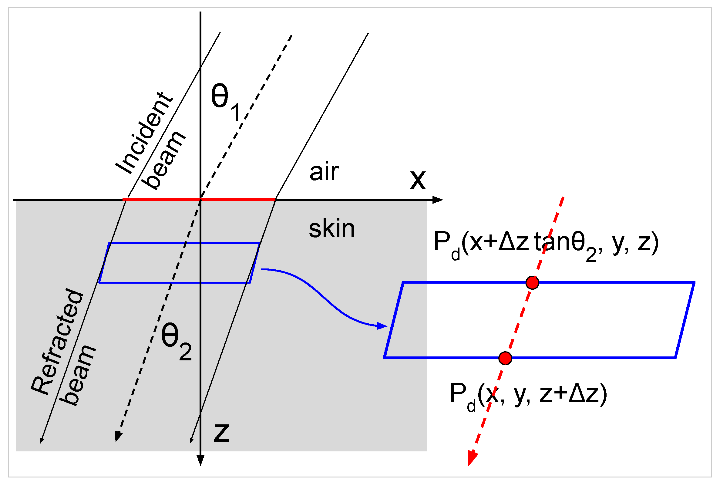
2.3. Beam Propagation and Power Absorption in Skin

As given in (11), for a Gaussian beam at an incident angle ${\theta }_1$, the power density projected onto the skin surface retains a two-dimensional Gaussian profile, albeit with a reduced beam center power density and elongated beam spot due to the oblique incidence. We examine the propagation and absorption of electromagnetic power as the beam penetrates the skin surface and continues into the underlying tissue layers.

Let $\alpha$ be the fraction of the incident beam power that passes through the skin surface (the remaining power is reflected). The power density passing through the skin surface is therefore given by $\alpha P_d^{\left(\mathrm{proj}\right)}(x,y)$ [10]. Let ${\theta }_2$ denote the angle of refraction, defined as the angle between the z-axis and the direction of beam propagation inside the skin (see Figure 4). The incident angle ${\theta }_1$ and the refracted angle ${\theta }_2$ are related by Snell’s law:

$${\displaystyle \frac{sin{\theta }_1}{sin{\theta }_2}}={\displaystyle \frac{n_{\mathrm{skin}}}{n_{\mathrm{air}}}}$$

(13)

where $n_{\mathrm{skin}}\approx 1.4$ and $n_{\mathrm{air}}\approx 1.0$ are the refractive indices of skin and air, respectively [11,12,13]. Since $n_{\mathrm{skin}}>n_{\mathrm{air}}$, the refracted angle is smaller than the incident angle, i.e., ${\theta }_2<{\theta }_1$.

Let $P_d(x,y,z)$ denote the power flux at position $(x,y,z)$, defined as the power per area passing through the plane parallel to the skin surface at depth z. Note that this plane is not perpendicular to the beam axis. Thus, $P_d(x,y,z)$ represents the power per unit area on an angled cross-section that is obliquely oriented relative to the beam’s direction of propagation (see Figure 4). Inside the skin, the beam rays follow straight-line paths described by $x\left(z\right)=x_{\mathrm{surf}}-ztan{\theta }_2,y\left(z\right)=y_{\mathrm{surf}}$. For the beam ray passing through point $(x,y,z)$ inside the skin, the corresponding entry point on the skin surface can be determined by tracing the beam ray backward to its intersection with the skin surface. This gives the following relations:

$$x_{\mathrm{surf}}=x+ztan{\theta }_2,y_{\mathrm{surf}}=y$$

At the skin surface ($z=0$), using $P_d(x,y,0)=\alpha P_d^{\left(\mathrm{proj}\right)}(x,y)$ and (11), we have

$$\begin{array}{cc}\hfill & P_d(x,y,0)=P_d^{\left(a\right)}f(x,y,{\sigma }_{\xi },{\sigma }_{\eta },{\varphi }_2)\hfill \\ \hfill & \mathrm{where}{P}_d^{\left(a\right)}\equiv \left(\alpha P_d^{\left(\mathrm{proj}\right)}\right)=(\alpha cos{\theta }_1{P}_d^{\left(i\right)})\hfill \end{array}$$

(14)

Here, $P_d^{\left(\mathrm{proj}\right)}$ represents the beam center power density arriving at the skin surface, while $P_d^{\left(a\right)}$ is the beam center power density that passes through the skin surface and is subsequently absorbed into the skin. $P_d^{\left(i\right)}$ denotes the beam center power density through a perpendicular cross-section in air, which is an intrinsic beam property independent of the incident angle. It is important to note that the skin surface is neither perpendicular to the incident beam in air nor to the refracted beam inside the skin. $f(x,y,{\sigma }_{\xi },{\sigma }_{\eta },{\varphi }_2)$ is the relative distribution of the power density projected onto the skin surface given in (11).

As the beam propagates through the skin, some electromagnetic power is absorbed. At depth z, $P_d(x,y,z)$ represents the remaining portion of $P_d(x+ztan{\theta }_2,y,0)$ from $z=0$ that has survived the absorption. According to the Beer–Lambert Law, the power absorption per unit length of propagation is proportional to the remaining power. From the skin surface to depth z, the propagation distance of the refracted beam is $(z/cos{\theta }_2)$. Applying the Beer–Lambert Law, the power density at depth z is given by the following:

$$P_d(x,y,z)=P_d(x+ztan{\theta }_2,y,0)e^{-{\displaystyle \frac{\mu }{cos{\theta }_2}}z}=P_d^{\left(a\right)}f(x+ztan{\theta }_2,y)e^{-{\displaystyle \frac{\mu }{cos{\theta }_2}}z}$$

(15)

where $\mu$ is the skin absorption coefficient for the electromagnetic frequency used. The propagation of the refracted beam and the power density $P_d(x,y,z)$ inside the skin are illustrated in Figure 4. We calculate the power absorbed per skin volume, which becomes the heating source. Consider a small parallelepiped defined by three pairs of parallel planes: $y=y_c\pm (\Delta y)/2$, $z=z_c\pm (\Delta z)/2$, and $x=x_c\pm (\Delta x)/2+ztan{\theta }_2$. The volume of this parallelepiped is $(\Delta x)(\Delta y)(\Delta z)$. The net power going into the parallelepiped is obtained by differentiating the power flux $P_d(x,y,z)$ with respect to z.

$$\begin{array}{cc}\hfill & (\Delta x)(\Delta y)P_d(x_c,y_c,z){|}_{z=z_c+(\Delta z)/2}^{z=z_c-(\Delta z)/2}\approx -(\Delta x)(\Delta y)(\Delta z){\displaystyle \frac{\partial P_d(x_c,y_c,z)}{\partial z}}{|}_{z=z_c}\hfill \\ \hfill & \approx (\Delta x)(\Delta y)(\Delta z)P_d^{\left(a\right)}f(x_c+z_{c}tan{\theta }_2,y_c){\displaystyle \frac{\mu }{cos{\theta }_2}}{e}^{-{\displaystyle \frac{\mu }{cos{\theta }_2}}z}\hfill \end{array}$$

Based on conservation of energy, the power absorbed per volume at $(x,y,z)$ is given by the net power going into the small parallelepiped divided by its volume $(\Delta x)(\Delta y)(\Delta z)$:

$$\begin{array}{|c|}\hline \left(\begin{array}{c}\mathrm{power}\mathrm{absorbed}\\ \mathrm{per}\mathrm{volume}\end{array}\right)=P_d^{\left(a\right)}f(x+ztan{\theta }_2,y){\displaystyle \frac{\mu }{cos{\theta }_2}}{e}^{-{\displaystyle \frac{\mu }{cos{\theta }_2}}z}\\ \hline\end{array}$$

(16)

Equation (16) gives the heat source in the skin temperature evolution. Note that (16) decays exponentially with respect to z, with a characteristic penetration depth of $1/\mu$. Therefore, the effect of the heat source is practically confined to a few multiples of $1/\mu$ in depth.

2.4. Skin Temperature Evolution

Let $T(x,y,z,t)$ denote the skin temperature at position $(x,y,z)$ at time t. To establish the governing equation for $T(x,y,z,t)$, we proceed with the following assumptions.

• The skin’s material properties are uniform in space, independent of $(x,y,z)$.
• The skin temperature prior to electromagnetic exposure is uniform in space, which is called the baseline skin temperature and denoted by $T_{\mathrm{base}}$.
• The electromagnetic power input per area at the skin surface is much larger than the rate of heat loss at the skin surface due to black body radiation, evaporation, or convective cooling by air. As a result, in the model formulation, we neglect the heat loss at the skin surface.
• The thickness of skin tissue is much larger than both the electromagnetic penetration depth and the thermal diffusion depth over the short exposure duration. As a result, in the model formulation, we treat the skin as a semi-infinite domain extending in the depth direction to $z=+\infty$.

Out of the four assumptions above, assumptions 1 and 2 are for the purpose of making the analytical solution tractable. The advantage of having an analytical solution is that the thermal effect of incident angle can be investigated systematically in an analytical framework for a short time, for a long time, and for various other parameter settings. Assumption 3 is well justified for high intensity short time electromagnetic exposures. Assumption 4 is also well justified since the skin tissue we consider is much thicker than the characteristic penetration depth $z_s=0.16\mathrm{mm}$ of a 95 GHz electromagnetic beam into skin tissue [14]. Relative to this characteristic penetration depth, the skin tissue can be mathematically modeled as semi-infinite in the z-direction.

The governing equation for $T(x,y,z,t)$ is derived from conservation of energy. The initial and boundary conditions for $T(x,y,z,t)$ follow directly from Assumptions 2 and 3.

$$\begin{gathered} \left\{\begin{array}{c}\underset{\mathrm{rate}\mathrm{of}\mathrm{change} \\ \mathrm{of}\mathrm{heat}\mathrm{in}\mathrm{skin}}{\underbrace{{\rho }_m{C}_p{\displaystyle \frac{\partial T}{\partial t}}}}=\underset{\mathrm{heat}\mathrm{flux}\mathrm{from} \\ \mathrm{conduction}}{\underbrace{k\left({\displaystyle \frac{{\partial }^{2}T}{\partial x^2}}+{\displaystyle \frac{{\partial }^{2}T}{\partial y^2}}+{\displaystyle \frac{{\partial }^{2}T}{\partial z^2}}\right)}}+\underset{\mathrm{heat}\mathrm{source}\mathrm{from} \\ \mathrm{absorbed}\mathrm{power}}{\underbrace{P_d^{\left(a\right)}f(x+ztan{\theta }_2,y){\displaystyle \frac{\mu }{cos{\theta }_2}}{e}^{-{\displaystyle \frac{\mu }{cos{\theta }_2}}z}}}\hfill \\ {\displaystyle \frac{\partial T(x,y,z,t)}{\partial z}{|}_{z=0}=0}\hfill \\ T(x,y,z,0)=T_{\mathrm{base}}\hfill \end{array}\right. \end{gathered}$$

(17)

In (17), ${\rho }_m$ denotes the mass density, $C_p$ the specific heat capacity, and k the heat conductivity of the skin. The quantity $P_d^{\left(a\right)}\equiv (\alpha cos{\theta }_1{P}_d^{\left(i\right)})$ represents the power per unit area transmitted through the skin surface at the beam center. ${\theta }_1$ is the incident angle and ${\theta }_2$ is the refracted angle of the electromagnetic beam. $\mu$ is the skin absorption coefficient at the relevant electromagnetic frequency. (17) is the initial boundary value problem (IBVP) governing the evolution of the skin temperature $T(x,y,z,t)$.

3. Analytical Solution of Skin Temperature

3.1. Nondimensionalization

We first establish appropriate scales to nondimensionalize the physical quantities in (17). The electromagnetic heat source term in (17) exhibits exponential decay with depth. The characteristic decay depth, $z_s\equiv 1/\mu$, serves as the natural length scale in the depth direction. In the lateral directions, the heat source varies with $f(x,y;{\sigma }_{\xi },{\sigma }_{\eta },{\varphi }_2)$, the 2D Gaussian relative distribution of power density projected onto the skin surface. It is tempting to select either the half-major axis ${\sigma }_{\xi }$ or the half-minor axis ${\sigma }_{\eta }$ in $f(x,y)$ as the length scale in the lateral directions. However, our objective is to develop a nondimensional formulation that enables studying the effects of incident angle and beam spot geometry. To accomplish this, the nondimensionalization process itself must be designed to be independent of both the incident angle and the specific geometry of the beam spot. This design requirement ensures that the influence of these parameters is fully captured in the resulting nondimensional formulation, allowing for meaningful comparative analysis. To that end, we introduce a representative lateral length scale, $r_s$, which reflects the overall lateral variation but remains unchanged when the incident angle and/or the specific beam spot geometry are varied. Fixing $r_s$ allows for a consistent nondimensionalization process across a family of beams, preserving the effects of beam geometry variations in the system after nondimensionalization. For instance, in a class of beams with an intrinsic beam radius about $5\mathrm{cm}$, we set $r_s=5\mathrm{cm}$. Even when the actual beam radius varies from $3\mathrm{cm}$ to $7\mathrm{cm}$ within this group, the lateral length scale remains fixed, and the effects of these variations are fully captured in the resulting nondimensional systrem. For the same reason, we have set the depth scale to $1/\mu$, rather than $(cos{\theta }_2/\mu )$.

For a 95 GHz electromagnetic beam, the absorption coefficient is $\mu =6250{\mathrm{m}}^{-1}$, yielding a characteristic depth scale of $z_s=1/\mu =0.16\mathrm{mm}$ [14]. In most applications, the size of the beam spot cross-section is several centimeters or larger [7,15,16,17]. Consequently, the lateral length scale is much larger than the depth scale: $r_s\gg z_s$. Since the effect of heat conduction is inversely proportional to the square of the length scale, its dominant effect of heat conduction occurs in the depth direction while its effect in the lateral directions is negligible. As a result, the time scale of heat conduction is determined by that in the depth direction: ${\displaystyle t_s=\frac{z_s^2}{(k/{\rho }_m{C}_p)}=\frac{{\rho }_m{C}_p}{k{\mu }^2}}$.

The temperature scale is defined as $\Delta T_s=(T_{\mathrm{act}}-T_{\mathrm{base}})$, where $T_{\mathrm{act}}$ is the activation temperature of thermal nociceptors [18]. This scale represents the temperature increase required to activate nociceptors. Below, we list the scales for relevant physical quantities and the resulting nondimensional quantities. To facilitate the subsequent analysis, we use the simple notation X without the subscript _nondim for all nondimensional quantities. For clarity, the original physical quantities are denoted by $X_{\mathrm{phy}}$.

$$\left\{\begin{array}{c}{\displaystyle z_s\equiv \frac{1}{\mu },z\equiv \frac{z_{\mathrm{phy}}}{z_s}}\hfill \\ {\displaystyle r_s\equiv \left(\mathrm{lateral}\mathrm{length}\mathrm{scale}\right),(x,y)\equiv \frac{(x_{\mathrm{phy}},y_{\mathrm{phy}})}{r_s}}\hfill \\ {\displaystyle ({\sigma }_1,{\sigma }_2,{\sigma }_{\xi },{\sigma }_{\eta })\equiv \frac{1}{r_s}{({\sigma }_1,{\sigma }_2,{\sigma }_{\xi },{\sigma }_{\eta })}_{\mathrm{phy}}}\hfill \\ {\displaystyle t_s\equiv \frac{{\rho }_m{C}_p}{k{\mu }^2},t\equiv \frac{t_{\mathrm{phy}}}{t_s}}\hfill \\ {\displaystyle T_s\equiv (T_{\mathrm{act},\mathrm{phy}}-T_{\mathrm{base},\mathrm{phy}}),T\equiv \frac{T_{\mathrm{phy}}-T_{\mathrm{base},\mathrm{phy}}}{T_s}}\hfill \\ {\displaystyle P_s\equiv k\mu T_s,P_{\mathrm{d}}^{\left(i\right)}\equiv \frac{P_{\mathrm{d},\mathrm{phy}}^{\left(i\right)}}{P_s},P_d^{\left(a\right)}\equiv \frac{P_{\mathrm{d},\mathrm{phy}}^{\left(a\right)}}{P_s}=(\alpha cos{\theta }_1{P}_d^{\left(i\right)})}\hfill \\ {\displaystyle f(x,y;{\sigma }_{\xi },{\sigma }_{\eta },{\varphi }_2)\equiv f_{\mathrm{phy}}(x_{\mathrm{phy}},y_{\mathrm{phy}};{\sigma }_{\xi ,\mathrm{phy}},{\sigma }_{\eta ,\mathrm{phy}},{\varphi }_2)}\hfill \end{array}\right.$$

(18)

Note that since all lateral length quantities are normalized by $r_s$, the functional form of $f(x,y)$ remains unchanged after nondimensionalization.

Substituting (18) into (17), we obtain the nondimensional IBVP for $T(x,y,z,t)$.

$$\left\{\begin{array}{c}{\displaystyle \frac{\partial T}{\partial t}={\epsilon }^2\left(\frac{{\partial }^{2}T}{\partial x^2}+\frac{{\partial }^{2}T}{\partial y^2}\right)+\frac{{\partial }^{2}T}{\partial z^2}+P_d^{\left(a\right)}f(x+\epsilon ztan{\theta }_2,y)\frac{1}{\lambda }{e}^{-z/\lambda },\lambda \equiv cos{\theta }_2}\hfill \\ {\displaystyle \frac{\partial T(x,y,z,t)}{\partial z}{|}_{z=0}=0}\hfill \\ {\displaystyle T(x,y,z,0)=0}\hfill \end{array}\right.$$

(19)

where ${\displaystyle \epsilon \equiv \frac{z_s}{r_s}}$ is the ratio of depth scale to lateral scale. In most applications, $\epsilon \ll 1$. In the nondimensionalization process outlined in (18), all scalings are independent of the incident angle ${\theta }_1$ and independent of a particular beam geometry. As a result, the effects of ${\theta }_1$ and beam geometry are fully retained in the nondimensional IBVP presented in (19). Specifically, in (19), the following items are affected by ${\theta }_1$.

$$\begin{array}{cc}\hfill & P_d^{\left(a\right)}=(\alpha cos{\theta }_1{P}_d^{\left(i\right)}),{\theta }_2=arcsin({\displaystyle \frac{n_{\mathrm{air}}}{n_{\mathrm{skin}}}}sin{\theta }_1),\lambda =cos{\theta }_2\hfill \\ \hfill & f(x,y)=f\left(x,y;\left[{\sigma }_{\xi },{\sigma }_{\eta },{\varphi }_2\right]({\sigma }_1,{\sigma }_2,\varphi ,{\theta }_1)\right)\hfill \end{array}$$

(20)

3.2. Asymptotic Solution of the Skin Temperature

The presence of the small parameter ${\displaystyle \epsilon \equiv \frac{z_s}{r_s}\ll 1}$ in (19) suggests a solution of the form

$$T(x,y,z,t)=T^{\left(0\right)}(x,y,z,t)+\epsilon T^{\left(1\right)}(x,y,z,t)+\dots$$

(21)

where $T^{\left(0\right)}$ and $T^{\left(1\right)}$ represent the leading-order and first-order terms in the asymptotic expansion, respectively. In this study, we focus on the leading-order term $T^{\left(0\right)}(x,y,z,t)$. Substituting the asymptotic solution (21) into the IBVP (19) and balancing the $O\left(1\right)$ terms, we obtain the governing IBVP for $T^{\left(0\right)}(x,y,z,t)$:

$$\left\{\begin{array}{c}{\displaystyle \frac{\partial T^{\left(0\right)}}{\partial t}=\frac{{\partial }^2{T}^{\left(0\right)}}{\partial z^2}+P_d^{\left(a\right)}f(x,y)\frac{1}{\lambda }{e}^{-z/\lambda },\lambda \equiv cos{\theta }_2}\hfill \\ {\displaystyle \frac{\partial T^{\left(0\right)}(x,y,z,t)}{\partial z}{|}_{z=0}=0}\hfill \\ {\displaystyle T^{\left(0\right)}(x,y,z,0)=0}\hfill \end{array}\right.$$

(22)

The governing IBVP (22) for $T^{\left(0\right)}(x,y,z,t)$ has several key properties:

• The forcing term (the heat source) in the differential equation $P_d^{\left(a\right)}f(x,y){\displaystyle \frac{1}{\lambda }}{e}^{-z/\lambda }$ has separate dependences on variable z and variables $(x,y)$.
• Equation (22) does not involve any derivatives with respect to $(x,y)$. As a result, Equation (22) can be viewed as an IBVP in variables $(z,t)$ with $(x,y)$ as parameters.
• The differential equation, boundary, and initial conditions are linear in $T^{\left(0\right)}$.
• The boundary and initial conditions are homogeneous.

With the properties above, we can take care of the forcing term in (22) using the principle of superposition. It follows that the solution $T^{\left(0\right)}(x,y,z,t)$ of (22) also has separate dependences on variable z and variables $(x,y)$. Specifically, it has the following form:

$$T^{\left(0\right)}(x,y,z,t)=P_d^{\left(a\right)}f(x,y)W^{\left(0\right)}(z,t;\lambda )$$

(23)

where $f(x,y)$ captures the spatial variation in skin temperature in lateral directions, and $W^{\left(0\right)}(z,t;\lambda )$ describes the evolution of skin temperature along the depth direction. $W^{\left(0\right)}$ is governed by the IBVP below in variables $(z,t)$ with $\lambda =cos{\theta }_2$ as a parameter.

$$\left\{\begin{array}{c}{\displaystyle \frac{\partial W^{\left(0\right)}}{\partial t}=\frac{{\partial }^2{W}^{\left(0\right)}}{\partial z^2}+\frac{1}{\lambda }{e}^{-z/\lambda }}\hfill \\ {\displaystyle \frac{\partial W^{\left(0\right)}(z,t)}{\partial z}{|}_{z=0}=0}\hfill \\ {\displaystyle W^{\left(0\right)}(z,0)=0}\hfill \end{array}\right.$$

(24)

In the scenario where the incident beam is perpendicular to the skin surface, we have ${\theta }_1={\theta }_2=0$ and $\lambda =cos{\theta }_2=1$. Previously, we solved (24) in the case of $\lambda =1$ [19].

$$\begin{array}{|c|}\hline \begin{array}{cc}\hfill & U^{\left(0\right)}(z,t)\equiv W^{\left(0\right)}(z,t;\lambda =1)=-e^{-z}+{\displaystyle \frac{e^{-z+t}}{2}}\mathrm{erfc}\left({\displaystyle \frac{-z+2t}{\sqrt{4t}}}\right)\hfill \\ \hfill & +{\displaystyle \frac{e^{z+t}}{2}}\mathrm{erfc}\left({\displaystyle \frac{z+2t}{\sqrt{4t}}}\right)-z\mathrm{erfc}\left({\displaystyle \frac{z}{\sqrt{4t}}}\right)+{\displaystyle \frac{2\sqrt{t}}{\sqrt{\pi }}}{e}^{{\displaystyle \frac{-z^2}{4t}}}\hfill \end{array}\\ \hline\end{array}$$

(25)

Note that $U^{\left(0\right)}(z,t)$ is a function of $(z,t)$ only, independent of any parameter. For the general case of $\lambda >0$, we scale variables $(z,t)$ and function $W^{\left(0\right)}(z,t;\lambda )$ as follows:

$$(\tilde{z},\tilde{t})\equiv ({\displaystyle \frac{z}{\lambda }},{\displaystyle \frac{t}{{\lambda }^2}}),\tilde{W}(\tilde{z},\tilde{t};\lambda )\equiv {\displaystyle \frac{1}{\lambda }}{W}^{\left(0\right)}(z,t;\lambda )$$

(26)

We use the chain rule to express derivatives of $W^{\left(0\right)}$ with respect to $(z,t)$ in terms of derivatives of $\tilde{W}$ with respect to $(\tilde{z},\tilde{t})$. It is straightforward to verify that for any $\lambda >0$, $\tilde{W}(\tilde{z},\tilde{t};\lambda )$ satisfies IBVP (24) with $\lambda =1$. Thus, $\tilde{W}(\tilde{z},\tilde{t};\lambda )$ is independent of $\lambda$, and we have $\tilde{W}(\tilde{z},\tilde{t};\lambda )=U^{\left(0\right)}(\tilde{z},\tilde{t})$. Using (26), we express $W^{\left(0\right)}$ in terms of $U^{\left(0\right)}$:

$$W^{\left(0\right)}(z,t;\lambda )=\lambda U^{\left(0\right)}(\tilde{z},\tilde{t}){|}_{(\tilde{z},\tilde{t})=({\displaystyle \frac{z}{\lambda }},{\displaystyle \frac{t}{{\lambda }^2}})}$$

(27)

Combining (23) and (27), we obtain the leading-order asymptotic solution to the IBVP (19).

$$\begin{array}{|c|}\hline \begin{array}{cc}\hfill & T^{\left(0\right)}(x,y,z,t;P_d^{\left(i\right)},{\sigma }_1,{\sigma }_2,\varphi ,{\theta }_1)=P_d^{\left(a\right)}f(x,y;{\sigma }_{\xi },{\sigma }_{\eta },{\varphi }_2)\lambda U^{\left(0\right)}(\tilde{z},\tilde{t}){|}_{(\tilde{z},\tilde{t})=({\displaystyle \frac{z}{\lambda }},{\displaystyle \frac{t}{{\lambda }^2}})}\hfill \\ \hfill & \mathrm{where}{P}_d^{\left(a\right)}=\left(\alpha P_d^{\left(\mathrm{proj}\right)}\right)=(\alpha cos{\theta }_1{P}_d^{\left(i\right)})\mathrm{and}\lambda =cos{\theta }_2\hfill \end{array}\\ \hline\end{array}$$

(28)

In solution expression (28), ${\theta }_1$ is the incident angle of the electromagnetic beam with respect to the skin surface. The intrinsic beam parameters $(P_d^{\left(i\right)},{\sigma }_1,{\sigma }_2,\varphi )$ are independent of the incident angle. On the right side of (28), there are several derived parameters.

• $P_d^{\left(a\right)}$: the beam center power density projected onto the skin surface and passing into the skin. $\alpha$ is the fraction of the arriving power passing into the skin.
• $f(x,y;{\sigma }_{\xi },{\sigma }_{\eta },{\varphi }_2)$: the relative distribution of power density projected onto the skin surface as a function of normalized variables $(x,y)$, given in (11).
• $({\sigma }_{\xi },{\sigma }_{\eta },{\varphi }_2)$: the geometric parameters describing the beam spot projected onto the skin surface. $({\sigma }_{\xi },{\sigma }_{\eta },{\varphi }_2)$ are calculated from the intrinsic beam parameters $({\sigma }_1,{\sigma }_2,\varphi )$ and the incident angle ${\theta }_1$, as described in (9) and (5).

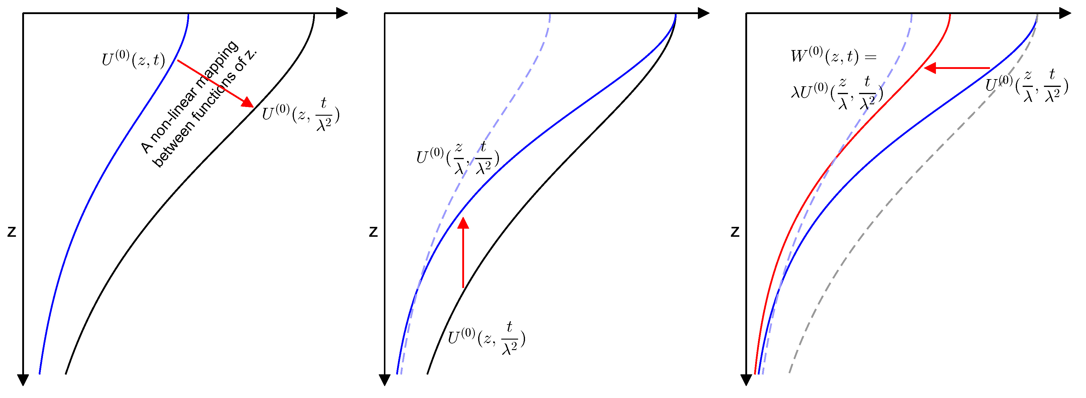
4. Scaling Properties

4.1. Scaling in 3D Skin Temperature

We consider the two beam setups described in (12): the original beam setup at a general incident angle with parameters $(P_d^{\left(i\right)},{\sigma }_1,{\sigma }_2,\varphi ,{\theta }_1)$, and the projected beam setup perpendicular to the skin surface with parameters $(P_d^{\left(\mathrm{proj}\right)},{\sigma }_{\xi },{\sigma }_{\eta },{\varphi }_2,{\theta }_1=0)$, where $P_d^{\left(\mathrm{proj}\right)}=cos{\theta }_1{P}_d^{\left(i\right)}$ and $({\sigma }_{\xi },{\sigma }_{\eta },{\varphi }_2)$ are calculated from $({\sigma }_1,{\sigma }_2,\varphi ,{\theta }_1)$ in (9) and (5). The original and projected beams share the same power density projected onto the skin surface. They differ in incident angle, in intrinsic power density, and in intrinsic geometric parameters over their respective perpendicular beam cross-sections.

For the original beam, the 3D skin temperature distribution as a function of $(x,y,z,t)$ is given directly in (28). This solution is valid for the arbitrary incident angle ${\theta }_1$ and arbitrary intrinsic beam parameters $(P_d^{\left(i\right)},{\sigma }_1,{\sigma }_2,\varphi )$. This solution expression is also applicable to the projected beam. For the projected beam, the incident angle is ${\theta }_1=0$, resulting in ${\theta }_2=0$ and $cos{\theta }_2=1$. When this already projected beam is projected again onto the skin surface, both the power density and the beam spot geometry remain unchanged.

$$\left\{\begin{array}{c}(\alpha cos{\theta }_1{P}_d^{\left(\mathrm{proj}\right)}){|}_{{\theta }_1=0}=\left(\alpha P_d^{\left(\mathrm{proj}\right)}\right)\hfill \\ \left[{\sigma }_{\xi },{\sigma }_{\eta },{\varphi }_2\right]({\sigma }_{\xi },{\sigma }_{\eta },{\varphi }_2,0)=[{\sigma }_{\xi },{\sigma }_{\eta },{\varphi }_2]\hfill \end{array}\right.$$

It follows that for the projected beam, the 3D skin temperature distribution is

$$T^{\left(0\right)}(x,y,z,t;P_d^{\left(\mathrm{proj}\right)},{\sigma }_{\xi },{\sigma }_{\eta },{\varphi }_2,0)=\left(\alpha P_d^{\left(\mathrm{proj}\right)}\right)f(x,y;{\sigma }_{\xi },{\sigma }_{\eta },{\varphi }_2)U^{\left(0\right)}(z,t)$$

(29)

The 3D temperature distribution (28) for the original beam is analogous to (29) for the projected beam. They are related through scalings in variables $(z,t)$ and in function value $U^{\left(0\right)}$. We compare them to highlight the similarities and the differences.

$$\left\{\begin{array}{cc}\stackrel{\begin{array}{c}3\mathrm{D}\mathrm{temperature}\mathrm{for}\\ \mathrm{the}\mathrm{original}\mathrm{beam}\end{array}}{\overbrace{T^{(0,\mathrm{orig})}(x,y,z,t)}}\hfill & \equiv T^{\left(0\right)}(x,y,z,t;P_d^{\left(i\right)},{\sigma }_1,{\sigma }_2,\varphi ,{\theta }_1)\hfill \\ & =\left(\alpha P_d^{\left(\mathrm{proj}\right)}\right)f(x,y;{\sigma }_{\xi },{\sigma }_{\eta },{\varphi }_2)\lambda U^{\left(0\right)}(\tilde{z},\tilde{t}){|}_{(\tilde{z},\tilde{t})=({\displaystyle \frac{z}{\lambda }},{\displaystyle \frac{t}{{\lambda }^2}})}\hfill \\ \stackrel{\begin{array}{c}3\mathrm{D}\mathrm{temperature}\mathrm{for}\\ \mathrm{the}\mathrm{projected}\mathrm{beam}\end{array}}{\overbrace{T^{(0,\mathrm{proj})}(x,y,z,t)}}\hfill & \equiv T^{\left(0\right)}(x,y,z,t;P_d^{\left(\mathrm{proj}\right)},{\sigma }_{\xi },{\sigma }_{\eta },{\varphi }_2,0)\hfill \\ & =\left(\alpha P_d^{\left(\mathrm{proj}\right)}\right)f(x,y;{\sigma }_{\xi },{\sigma }_{\eta },{\varphi }_2)U^{\left(0\right)}(z,t)\hfill \end{array}\right.$$

(30)

When we treat them as functions of $(x,y,z,t)$, we can start from the temperature distribution of the projected beam $T^{(0,\mathrm{proj})}(x,y,z,t)$ and obtain the temperature distribution of the original beam $T^{(0,\mathrm{orig})}(x,y,z,t)$ as follows:

• Scale the z-direction by a factor of $\lambda \equiv cos{\theta }_2$.
• Scale the t-direction by a factor of ${\lambda }^2$.
• Scale the function value by a factor of $\lambda$.

For example, the point $({\displaystyle \frac{z}{\lambda }},{\displaystyle \frac{t}{{\lambda }^2}})$ in $T^{(0,\mathrm{proj})}(x,y,z,t)$ before scaling becomes the point $(z,t)$ after scaling. As functions of $(x,y,z,t)$, $T^{(0,\mathrm{orig})}(x,y,z,t)$ and $T^{(0,\mathrm{proj})}(x,y,z,t)$ are related by

$$\begin{array}{|c|}\hline T^{(0,\mathrm{orig})}(x,y,z,t)=\lambda T^{(0,\mathrm{proj})}(x,y,{\displaystyle \frac{z}{\lambda }},{\displaystyle \frac{t}{{\lambda }^2}}),\lambda =cos{\theta }_2\\ \hline\end{array}$$

(31)

Scaling law (31) corresponds to the mapping from $U^{\left(0\right)}$ to $W^{\left(0\right)}$ in (27). Note that $T^{(0,\mathrm{proj})}$ and $U^{\left(0\right)}$ at time ${\displaystyle \frac{t}{{\lambda }^2}}$ are mapped to $T^{(0,\mathrm{orig})}$ and $W^{\left(0\right)}$ at time t. When we compare $U^{\left(0\right)}$ and $W^{\left(0\right)}$ at the same time level t, we need to view (27) as a mapping between two functions of z, instead of a mapping between two functions of $(z,t)$. Specifically, we view it as a mapping from $U^{\left(0\right)}(•,t)$ (a function of z at time t) to $W^{\left(0\right)}(•,t)$ (a function of z at time t). We dissect the mapping from $U^{\left(0\right)}(•,t)$ to $W^{\left(0\right)}(•,t)$ into three steps below:

$$\begin{array}{cc}\hfill & U^{\left(0\right)}(•,t)\stackrel{\mathrm{This}\mathrm{is}\mathrm{a}\mathrm{nonlinear}\mathrm{mapping}\mathrm{on}\mathrm{a}\mathrm{function}\mathrm{of}z.}{\to }{U}^{\left(0\right)}(•,{\displaystyle \frac{t}{{\lambda }^2}})\hfill \\ \hfill & U^{\left(0\right)}(•,{\displaystyle \frac{t}{{\lambda }^2}})\stackrel{\mathrm{This}\mathrm{is}\mathrm{a}\mathrm{linear}\mathrm{scaling}\mathrm{in}\mathrm{variable}z.}{\to }{U}^{\left(0\right)}({\displaystyle \frac{•}{\lambda }},{\displaystyle \frac{t}{{\lambda }^2}})\hfill \\ \hfill & U^{\left(0\right)}({\displaystyle \frac{•}{\lambda }},{\displaystyle \frac{t}{{\lambda }^2}})\stackrel{\mathrm{This}\mathrm{is}\mathrm{a}\mathrm{linear}\mathrm{scaling}\mathrm{in}\mathrm{function}\mathrm{value}.}{\to }\lambda U^{\left(0\right)}({\displaystyle \frac{•}{\lambda }},{\displaystyle \frac{t}{{\lambda }^2}})=W^{\left(0\right)}(•,t)\hfill \end{array}$$

(32)

The three steps of the mapping are illustrated in Figure 5. Notice that the first step is nonlinear when viewed as a mapping between two functions of z.

In summary, as two functions of $(x,y,z,t)$, the temperature distribution of the original beam at incident angle ${\theta }_1$, $T^{(0,\mathrm{orig})}(x,y,z,t)$, is obtained from the temperature distribution of the projected beam, $T^{(0,\mathrm{proj})}(x,y,z,t)$, via scalings in variables $(z,t)$ and in function value T. When comparing the two distributions in space at a fixed time t, there is a nonlinear step mapping $T^{(0,\mathrm{proj})}$ from time t to time ${\displaystyle \frac{t}{{\lambda }^2}}$.

4.2. Scaling of Skin Surface Heating Rates

Let $T^{\left(\mathrm{surf}\right)}(t;P_d^{\left(i\right)},{\theta }_1)$ denote the beam center temperature on the skin surface at time t, caused by a beam with intrinsic beam center power density $P_d^{\left(i\right)}$ at incident angle ${\theta }_1$. Notice that the beam center temperature is independent of $({\sigma }_1,{\sigma }_2,\varphi )$, the intrinsic geometric parameters of the beam spot. Intrinsic parameters $({\sigma }_1,{\sigma }_2,\varphi )$ affect the projected beam spot on the skin surface and the lateral distribution of 3D skin temperature, not the beam center temperature. Evaluating the 3D temperature solution (28) at the origin $(0,0,0)$ and using the fact that $f(0,0)=1$, we obtain the expression of $T^{\left(\mathrm{surf}\right)}(t;P_d^{\left(i\right)},{\theta }_1)$.

$$\begin{array}{cc}\hfill & T^{\left(\mathrm{surf}\right)}(t;P_d^{\left(i\right)},{\theta }_1)\equiv T^{\left(0\right)}(x,y,z,t;P_d^{\left(i\right)},{\theta }_1){|}_{(x,y,z)=(0,0,0)}=P_d^{\left(a\right)}\lambda h\left({\displaystyle \frac{t}{{\lambda }^2}}\right)\hfill \\ \hfill & \mathrm{where}{P}_d^{\left(a\right)}\equiv \left(\alpha P_d^{\left(\mathrm{proj}\right)}\right)=(\alpha cos{\theta }_1{P}_d^{\left(i\right)}),\lambda =cos{\theta }_2,\hfill \end{array}$$

(33)

and $h\left(t\right)$ is a parameter-free single-variable function defined as follows:

$$h\left(t\right)\equiv U^{\left(0\right)}(z,t){|}_{z=0}=\mathrm{erfc}\left(\sqrt{t}\right)e^t-1+{\displaystyle \frac{2}{\sqrt{\pi }}}\sqrt{t}$$

(34)

Equation (33) is the skin surface temperature for the original beam with power density $P_d^{\left(i\right)}$ and incident angle ${\theta }_1$. For the projected beam with power density $P_d^{\left(\mathrm{proj}\right)}$ and incident angle ${\theta }_1=0$, the skin surface temperature is

$$T^{\left(\mathrm{surf}\right)}(t;P_d^{\left(\mathrm{proj}\right)},0)=\alpha P_d^{\left(\mathrm{proj}\right)}h\left(t\right)$$

(35)

Comparing (33) and (35), we obtain the scaling law for $T^{\left(\mathrm{surf}\right)}$:

$$\begin{array}{|c|}\hline T^{\left(\mathrm{surf}\right)}(t;P_d^{\left(i\right)},{\theta }_1)=\lambda T^{\left(\mathrm{surf}\right)}({\displaystyle \frac{t}{{\lambda }^2}};P_d^{\left(\mathrm{proj}\right)},0),\lambda =cos{\theta }_2\\ \hline\end{array}$$

(36)

Next we study the rates of skin surface temperature increase caused by the original beam and by the projected beam. For small t and for large t, respectively, function $h\left(t\right)$ has the asymptotic behaviors below:

$$\left\{\begin{array}{c}{\displaystyle h\left(t\right)=t-\frac{4}{3\sqrt{\pi }}{t}^{3/2}+O\left(t^2\right)\mathrm{for}\mathrm{small}t}\hfill \\ {\displaystyle h\left(t\right)=\frac{2}{\sqrt{\pi }}\sqrt{t}-1+O\left(\frac{1}{\sqrt{t}}\right)\mathrm{for}\mathrm{large}t}\hfill \end{array}\right.$$

(37)

In experiments, the skin surface temperature is recorded with an infrared thermal camera at a sequence of time instances [15,16]. We use the rate of measured skin surface temperature increase to estimate $P_d^{\left(a\right)}$, the power density projected onto the skin surface and passing into the skin [20].

$$\begin{array}{cc}\hfill & {\displaystyle \frac{d}{dt}}{T}^{\left(\mathrm{surf}\right)}(t;P_d^{\left(i\right)},{\theta }_1)={\displaystyle \frac{P_d^{\left(a\right)}}{cos{\theta }_2}}\mathrm{for}\mathrm{small}t\hfill \end{array}$$

(38)

$$\begin{array}{ccc}\hfill & \left(\sqrt{\pi t}\right){\displaystyle \frac{d}{dt}}{T}^{\left(\mathrm{surf}\right)}(t;P_d^{\left(i\right)},{\theta }_1)=P_d^{\left(a\right)}\mathrm{for}\mathrm{large}t\hfill & \hfill \end{array}$$

(39)

If we use (39) for large t to estimate $P_d^{\left(a\right)}$, the estimate is unaffected by the incident angle. In contrast, if we use (38) for small t to estimate $P_d^{\left(a\right)}$ and we ignore the effect of incident angle, then $P_d^{\left(a\right)}$ is overestimated by a factor of $(1/cos{\theta }_2)$.

We now present two mathematical assertions on function $h\left(t\right)$, which will be used to compare surface temperatures caused by several beam setups at the same time level t.

(A1):

The function ${\displaystyle \frac{1}{\sqrt{s}}h\left(s\right)}$ is monotonically increasing for $s>0$.

(A2):

The function ${\displaystyle \frac{1}{s}h\left(s\right)}$ is monotonically decreasing for $s>0$.

Assertions (A1) and (A2) can be derived analytically. Here, we demonstrate their validity numerically. Figure 6 illustrates the graphs of ${\displaystyle \frac{1}{\sqrt{s}}h\left(s\right)}$ (left panel) and ${\displaystyle \frac{1}{s}h\left(s\right)}$ (right panel). The monotonic trend of each function is clearly evident in Figure 6.

For $\lambda <1$, we have $s=t/{\lambda }^2>t$. Assertions (A1) and (A2) imply, respectively,

$$\begin{array}{cc}\hfill & \left(\mathrm{A}1\right):{\displaystyle \frac{1}{\sqrt{s}}}h\left(s\right){|}_{s=t/{\lambda }^2}-{\displaystyle \frac{1}{\sqrt{t}}}h\left(t\right)>0⟹{\displaystyle \frac{1}{\sqrt{t}}}\left(\lambda h\left({\displaystyle \frac{t}{{\lambda }^2}}\right)-h\left(t\right)\right)>0\hfill \end{array}$$

$$\begin{array}{cc}\hfill & ⟹\lambda h\left({\displaystyle \frac{t}{{\lambda }^2}}\right)>h\left(t\right)\mathrm{for}\mathrm{any}\lambda <1.\hfill \end{array}$$

(40)

$$\begin{array}{cc}\hfill & \left(\mathrm{A}2\right):{\displaystyle \frac{1}{t}}h\left(t\right)-{\displaystyle \frac{1}{s}}h\left(s\right){|}_{s=t/{\lambda }^2}>0⟹{\displaystyle \frac{1}{t}}\left(h\left(t\right)-{\lambda }^{2}h\left({\displaystyle \frac{t}{{\lambda }^2}}\right)\right)>0\hfill \end{array}$$

$$\begin{array}{cc}\hfill & ⟹h\left(t\right)>{\lambda }^{2}h\left({\displaystyle \frac{t}{{\lambda }^2}}\right)\mathrm{for}\mathrm{any}\lambda <1.\hfill \end{array}$$

(41)

For $\lambda =cos{\theta }_2$, utilizing scaling law (36) and expression (33), we interpret inequalities (40) and (41) in terms of the skin surface temperature $T^{\left(\mathrm{surf}\right)}$ for three beam setups.

$$\begin{array}{cc}\hfill & T^{\left(\mathrm{surf}\right)}(t;P_d^{\left(i\right)},{\theta }_1)=\underset{\lambda h({\displaystyle \frac{t}{{\lambda }^2}})>h\left(t\right)}{\underbrace{\lambda T^{\left(\mathrm{surf}\right)}({\displaystyle \frac{t}{{\lambda }^2}};P_d^{\left(\mathrm{proj}\right)},0)>T^{\left(\mathrm{surf}\right)}(t;P_d^{\left(\mathrm{proj}\right)},0)}}\hfill \end{array}$$

(42)

$$\begin{array}{cc}\hfill & \underset{h\left(t\right)>{\lambda }^{2}h({\displaystyle \frac{t}{{\lambda }^2}})}{\underbrace{T^{\left(\mathrm{surf}\right)}(t;P_d^{\left(i\right)},0)>{\lambda }^2{T}^{\left(\mathrm{surf}\right)}({\displaystyle \frac{t}{{\lambda }^2}};P_d^{\left(i\right)},0)}}=\lambda T^{\left(\mathrm{surf}\right)}({\displaystyle \frac{t}{{\lambda }^2}};\left(\lambda P_d^{\left(i\right)}\right),0)\hfill \\ \hfill & >\lambda T^{\left(\mathrm{surf}\right)}({\displaystyle \frac{t}{{\lambda }^2}};P_d^{\left(\mathrm{proj}\right)},0)=T^{\left(\mathrm{surf}\right)}(t;P_d^{\left(i\right)},{\theta }_1)\hfill \end{array}$$

(43)

In (43), we have used $\lambda P_d^{\left(i\right)}=cos{\theta }_2{P}_d^{\left(i\right)}>cos{\theta }_1{P}_d^{\left(i\right)}=P_d^{\left(\mathrm{proj}\right)}$. We use (42) and (43) to compare the skin surface temperatures caused by three beam setups.

$$\begin{gathered} \begin{array}{|c|}\hline \underset{\mathrm{original}\mathrm{beam} \\ \mathrm{at}0\mathrm{incident}\mathrm{angle}}{\underbrace{T^{\left(\mathrm{surf}\right)}(t;P_d^{\left(i\right)},0)}}>\underset{\mathrm{original}\mathrm{beam} \\ \mathrm{at}\mathrm{incident}\mathrm{angle}{\theta }_1}{\underbrace{T^{\left(\mathrm{surf}\right)}(t;P_d^{\left(i\right)},{\theta }_1)}}>\underset{\mathrm{projected}\mathrm{beam} \\ \mathrm{at}0\mathrm{incident}\mathrm{angle}}{\underbrace{T^{\left(\mathrm{surf}\right)}(t;P_d^{\left(\mathrm{proj}\right)},0)}}\\ \hline\end{array} \end{gathered}$$

(44)

In (44), $P_d^{\left(i\right)}$ is the intrinsic beam center power density over a perpendicular beam cross-section of the original beam. $P_d^{\left(\mathrm{proj}\right)}=cos{\theta }_1{P}_d^{\left(i\right)}$ is the beam center power density of the original beam projected on the skin surface, which is also the beam center power density of the projected beam. (44) compares the skin surface temperatures at beam center at time t caused by three beam setups. The term in the middle is the surface temperature for the original beam setup (with intrinsic power density $P_d^{\left(i\right)}$ at incident angle ${\theta }_1$). The term on the right is the surface temperature for the projected beam setup (with power density $P_d^{\left(\mathrm{proj}\right)}=cos{\theta }_1{P}_d^{\left(i\right)}$ at zero incident angle). The term on the left is the surface temperature caused by the beam with power density $P_d^{\left(i\right)}$ at zero incident angle. This is the same intrinsic beam as the original beam but at zero incident angle. Inequality (44) states that, at any fixed time t, the surface temperature caused by a beam at incident angle ${\theta }_1$ is lower than the surface temperature caused by the same intrinsic beam at zero incident angle, but is higher than the surface temperature caused by the projected beam at zero incident angle.

4.3. Scaling of Activated Skin Volume

Thermal nociceptors in the skin are activated whenever the local skin temperature exceeds the activation threshold, denoted as $T_{\mathrm{act},\mathrm{phy}}$. This activation threshold is used in the definition of temperature scale $T_s\equiv T_{\mathrm{act},\mathrm{phy}}-T_{\mathrm{base},\mathrm{phy}}$ in (18). After nondimensionalization, the nondimensional activation temperature becomes $T_{\mathrm{act}}=1$. Let $V_{\mathrm{act}}\left(t\right)$ denote the volume of the skin region where thermal nociceptors are activated at time t.

$$V_{\mathrm{act}}\left(t\right)\equiv \mathrm{volume}\left\{(x,y,z)|T^{\left(0\right)}(x,y,z,t)\ge 1\right\}$$

(45)

We consider two beam setups described in (12): the original beam setup with parameters $(P_d^{\left(i\right)},{\sigma }_1,{\sigma }_2,\varphi ,{\theta }_1)$ and the projected beam setup with parameters $(P_d^{\left(\mathrm{proj}\right)},{\sigma }_{\xi },{\sigma }_{\eta },{\varphi }_2,{\theta }_1=0)$. As functions of $(x,y,z,t)$, the temperature distributions of the two beam setups are related by the scalings in (31): $T^{(0,\mathrm{orig})}(x,y,z,t)=\lambda T^{(0,\mathrm{proj})}(x,y,{\displaystyle \frac{z}{\lambda }},{\displaystyle \frac{t}{{\lambda }^2}})$.

In scaling law (31), the scaling in z translates to a scaling in the activated volume. The scaling in t relates the activated volume at one time to that at a different time. The activated skin volume is defined by the condition $T^{\left(0\right)}(x,y,z,t)\ge 1$ in (45), which is clearly not linear in T. As a result, the scaling in T does not produce a simple relation on the activated volume in a straightforward way. Notice that as given in (29), the skin temperature for the projected beam is proportional to $P_d^{\left(\mathrm{proj}\right)}$. To connect the activated skin volumes caused by the two beam setups, in (31), we move the scaling multiplier $\lambda =cos{\theta }_2$ on temperature T into the solution expression as a scaling multiplier on power density $P_d^{\left(\mathrm{proj}\right)}$. We consider the projected beam with scaled power density, described by parameters $\left(\lambda P_d^{\left(\mathrm{proj}\right)},{\sigma }_{\xi },{\sigma }_{\eta },{\varphi }_2,{\theta }_1=0\right)$. The temperature distributions of the original beam and the projected beam with scaled power density are related by scalings in $(z,t)$ only, with no scaling in T. Specifically, we have the following:

$$T^{\left(0\right)}(x,y,z,t;P_d^{\left(i\right)},{\sigma }_1,{\sigma }_2,\varphi ,{\theta }_1)=T^{\left(0\right)}(x,y,{\displaystyle \frac{z}{\lambda }},{\displaystyle \frac{t}{{\lambda }^2}};\lambda P_d^{\left(\mathrm{proj}\right)},{\sigma }_{\xi },{\sigma }_{\eta },{\varphi }_2,0)$$

(46)

Scaling law (46) leads to a scaling law on the activated volumes of the original beam and the projected beam with scaled power density as two functions of t.

$$\begin{array}{cc}\hfill & V_{\mathrm{act}}(t;P_d^{\left(i\right)},\left({\sigma }_1{\sigma }_2\right),{\theta }_1)=\lambda V_{\mathrm{act}}({\displaystyle \frac{t}{{\lambda }^2}};\lambda P_d^{\left(\mathrm{proj}\right)},\left({\sigma }_{\xi }{\sigma }_{\eta }\right),0)\hfill \end{array}$$

(47)

Note that, among the beam’s geometric parameters, the activated volume depends only on $\left({\sigma }_{\xi }{\sigma }_{\eta }\right)$, the area of the beam spot projected onto the skin surface. The azimuthal orientation angle ${\varphi }_2$ rotates the activated skin region but does not alter its volume. When the beam spot area is kept fixed, changing the beam aspect ratio ${\sigma }_{\xi }/{\sigma }_{\eta }$ stretches the activated skin region in one direction and shrinks it simultaneously by the same factor in the perpendicular direction, leaving the volume unchanged. The area of the projected beam spot on the skin surface is ${\sigma }_{\xi }{\sigma }_{\eta }={\sigma }_1{\sigma }_2/cos{\theta }_1$. Substituting $\lambda =cos{\theta }_2$, $P_d^{\left(\mathrm{proj}\right)}=cos{\theta }_1{P}_d^{\left(i\right)}$, and ${\sigma }_{\xi }{\sigma }_{\eta }={\sigma }_1{\sigma }_2/cos{\theta }_1$ into (47), we obtain the scaling law below.

$$\begin{gathered} \begin{array}{|c|}\hline \underset{\mathrm{original}\mathrm{beam}\mathrm{at}\mathrm{incident} \\ \mathrm{angle}{\theta }_1\mathrm{at}\mathrm{time}t}{\underbrace{V_{\mathrm{act}}(t;P_d^{\left(i\right)},\left({\sigma }_1{\sigma }_2\right),{\theta }_1)}}=\underset{\begin{array}{c}\mathrm{modified}\mathrm{beam}\mathrm{at}\mathrm{zero}\mathrm{incident}\\ \mathrm{angle}\mathrm{at}\mathrm{time}(t/{cos}^2{\theta }_2)\end{array}}{\underbrace{V_{\mathrm{act}}\left({\displaystyle \frac{t}{{cos}^2{\theta }_2}};(cos{\theta }_{2}cos{\theta }_1{P}_d^{\left(i\right)}),({\displaystyle \frac{cos{\theta }_2}{cos{\theta }_1}}{\sigma }_1{\sigma }_2),0\right)}}\\ \hline\end{array} \end{gathered}$$

(48)

For a beam at incident angle ${\theta }_1$, scaling law (48) states that its activated volume at time t is equal to the activated volume of a modified beam at an extended exposure time $(t/{cos}^2{\theta }_2)$. In the modified beam, the incident angle is zero. The intrinsic beam center power density is scaled by a factor of $cos{\theta }_{2}cos{\theta }_1<1$, and the intrinsic beam spot area is scaled by a factor of $cos{\theta }_2/cos{\theta }_1>1$. Here ${\theta }_2$ is the refracted angle corresponding to the incident angle ${\theta }_1$.

We examine the time at which a given threshold on the activated skin volume is reached. As noted earlier, the activated volume is proportional to the beam spot area. In the case of a very large beam spot area, the time to reach the volume threshold is approximately the time when the activation temperature $T_{\mathrm{act}}$ is reached. In the temperature distribution (28), the spatial maximum occurs at the beam center on the skin surface, which is denoted by $T^{\left(\mathrm{surf}\right)}$ and is given in (33). Before $T^{\left(\mathrm{surf}\right)}$ reaches $T_{\mathrm{act}}$, no skin region is activated. As time t increases, $T^{\left(\mathrm{surf}\right)}$ increases monotonically. When $T^{\left(\mathrm{surf}\right)}$ goes slightly above $T_{\mathrm{act}}$, the skin within a small depth becomes activated. This small activated depth, when multiplied by the very large beam spot area, produces an activated volume above the volume threshold. Let $t_{\mathrm{act}}$ denote the activation time, defined as the time when $T^{\left(\mathrm{surf}\right)}$ reaches $T_{\mathrm{act}}$ and the activated volume transitions from zero to positive.

$$t_{\mathrm{act}}(P_d^{\left(i\right)},{\theta }_1)\equiv min\left\{t|T^{\left(\mathrm{surf}\right)}(t;P_d^{\left(i\right)},{\theta }_1)\ge T_{\mathrm{act}}\right\}$$

(49)

In the case of a very large beam spot area, $t_{\mathrm{act}}(P_d^{\left(i\right)},{\theta }_1)$ is approximately the time when the activated volume reaches the volume threshold. In (44), we compared the skin surface temperatures at time t caused by three beam setups. The ordering of skin surface temperatures at fixed time t given in (44) leads to the corresponding ordering of activation times for the three beam setups.

$$\begin{gathered} \begin{array}{|c|}\hline \underset{\mathrm{original}\mathrm{beam} \\ \mathrm{at}0\mathrm{incident}\mathrm{angle}}{\underbrace{t_{\mathrm{act}}(P_d^{\left(i\right)},0)}}<\underset{\mathrm{original}\mathrm{beam} \\ \mathrm{at}\mathrm{incident}\mathrm{angle}{\theta }_1}{\underbrace{t_{\mathrm{act}}(P_d^{\left(i\right)},{\theta }_1)}}<\underset{\mathrm{projected}\mathrm{beam} \\ \mathrm{at}0\mathrm{incident}\mathrm{angle}}{\underbrace{t_{\mathrm{act}}(P_d^{\left(\mathrm{proj}\right)},0)}}\\ \hline\end{array} \end{gathered}$$

(50)

In (50), the term in the middle is the activation time for the original beam setup (with intrinsic power density $P_d^{\left(i\right)}$ at incident angle ${\theta }_1$). The term on the right is the activation time for the projected beam setup (with power density $P_d^{\left(\mathrm{proj}\right)}=cos{\theta }_1{P}_d^{\left(i\right)}$ at zero incident angle). The term on the left is the activation time for the beam with power density $P_d^{\left(i\right)}$ at zero incident angle. This is the same intrinsic beam as the original beam but at zero incident angle. Inequality (50) states that for a given beam at incident angle ${\theta }_1$, the time required to reach thermal nociceptor activation is longer than the activation time for the same beam at zero incident angle but is shorter than the activation time for the projected beam at zero incident angle.

5. Discussion

We studied the thermal effect on skin from an electromagnetic beam at an incident angle. We carried out nondimensionalization and solved the nondimensional formulation for a leading-term asymptotic solution. The asymptotic analysis is not based on the fact that the incident angle is small. Rather it is based on the fact that the depth scale is much smaller than the lateral scale. For a millimeter wavelength beam, the penetration depth of the electromagnetic wave is sub-millimeter, leading to concentrated heating in the top skin layer and a large temperature gradient in the depth direction. In contrast, in the lateral directions, the characteristic length is described by the size of beam spot, which spans at least several centimeters in applications. This separation of length scales in the depth and lateral directions makes the ratio of depth to lateral length scales a small parameter in the nondimensional formulation. One consequence of this small parameter is that the heat conduction in the lateral directions is negligible compared to that in the depth direction.

When skin is exposed to an electromagnetic beam at an incident angle, the beam’s power is first projected onto the skin surface. This projection affects the power per area over the skin surface, making it different from the power density over a perpendicular beam cross-section. This projection is included in the thermal model. A fraction of the power arriving at the skin surface is absorbed into the skin and continues propagating inside the skin along the refracted angle. Due to the refracted angle, the beam propagation distance is more than the depth and the power density absorption per depth is more than that in the case of a zero refracted angle. Also the power density (and thus the heating source) shifts laterally as the beam propagates into the skin. This lateral shift is comparable to the depth scale but is much smaller than the lateral length scale. The asymptotic analysis is based on the ratio of the depth scale to the lateral length scale being small, not on the incident angle being small. The asymptotic solution obtained is expressed in terms of parameter-free single-variable functions and is valid for any incident angle.

Based on the asymptotic solution, we investigated the thermal effects of three beam setups. Each beam setup is defined by the intrinsic parameters (power density, beam spot geometry) over a perpendicular beam cross-section and the incident angle. We examined the following three beam setups:

• Beam 1: the original beam at incident angle ${\theta }_1$.
• Beam 1v: the beam with the same intrinsic parameters as the original beam but at zero incident angle (i.e., the original intrinsic beam at zero incident angle).
• Beam 2: the projected beam at zero incident angle. The projected beam has the same power density projected onto the skin surface as the original beam (beam 1).

As described above, beams 1 and 2 share the same power density projected on the skin surface but have different incident angles; beams 1 and 1v share the same intrinsic power density over their respective perpendicular cross-section but have different incident angles; beam 2 has a lower power density and a larger beam spot area than beam 1v, although both are at zero incident angle. From the analysis, we obtained the results below.

• For the original beam at incident angle ${\theta }_1$ (beam 1), the electromagnetic heating source inside the skin decays in the depth direction faster than beams 1v and 2, which are both perpendicular to the skin surface. This is because the propagation distance per depth is longer for a beam ray along a refracted angle than for one along the depth directly. This increased path length results in a greater absorption and attenuation per depth of the electromagnetic wave as it propagates into the skin.
• The 3D skin temperature distribution as a function of $(x,y,z,t)$ caused by the original beam (beam 1) is related to that caused by the projected beam (beam 2) through scalings in variables $(z,t)$ and in temperature T. In particular, the temperature distribution of beam 1 at time t is related to that of beam 2 at the extended exposure time $(t/{cos}^2{\theta }_2)$, where ${\theta }_2$ is the refracted angle corresponding to the incident angle ${\theta }_1$.
• In exposure tests, the skin surface temperature is recorded at discrete time instances using an infrared thermal camera. For a beam perpendicular to the skin surface, the absorbed power density can be estimated from the measured rate of surface temperature increase at small times (t). In millimeter-wave (MMW) exposures, small t refers to the time period immediately after the start of exposure, within a fraction of the time scale. The time scale is the characteristic time of heat diffusion over the depth scale. Large t refers to time durations several multiples of this time scale after the start of exposure. For a beam at an incident angle, estimating the absorbed power density from the surface temperature increase rate at small t leads to an overestimation unless the incident angle is known and explicitly accounted for in the calculation. In contrast, using the surface temperature increase rate at large t yields an accurate estimate of the absorbed power density regardless of the incident angle.
• We analytically compared the skin surface temperatures induced by the three beam setups. At any fixed time t, the beam center temperature for the original beam (beam 1) is higher than the temperature for the projected beam (beam 2) but is lower than the temperature for beam 1v (the original intrinsic beam at zero incident angle). Given a beam with fixed intrinsic parameters, the most effective way to increase skin surface temperature is to set the incident angle to zero during exposure. On the other hand, when the power density projected onto the skin surface is fixed, which can be achieved by various beam setups, the skin surface temperature is higher if this fixed projected power density is achieved by a beam at a larger incident angle.
• In MMW exposures, thermal nociceptors in the skin are activated wherever the local temperature exceeds the activation threshold. The activated skin volume may be used to quantify the heat sensation transduced in the brain from nociceptive signals. The activated skin volume caused by the original beam at incident angle ${\theta }_1$ at time t is equal to that caused by a modified beam at zero incident angle at an extended exposure time of $t/{cos}^2{\theta }_2$, where ${\theta }_2$ is the refracted angle. In the modified beam, the intrinsic power density is reduced (multiplied by a factor of $cos{\theta }_{2}cos{\theta }_1<1$), and the intrinsic beam spot area is slightly increased (multiplied by a factor of $cos{\theta }_2/cos{\theta }_1>1$).
• We also examined the activation time, defined as the time when the thermal nociceptor activation temperature is first reached. For the original beam at incident angle ${\theta }_1$ (beam 1), the activation time is longer than that for the same intrinsic beam at zero incident angle (beam 1v), but is shorter than that for the projected beam (beam 2).

6. Conclusions

In summary, we formulated a simple mathematical model for the skin thermal effect of an electromagnetic beam at an arbitrary incident angle. Under the assumption that the lateral length scale is much larger than the characteristic penetration depth of the electromagnetic beam, we carried out an asymptotic analysis and obtained the leading term asymptotic solution. The asymptotic solution does not require a small incident angle. This analytical solution provides an analytical framework for investigating the skin thermal effect of an electromagnetic beam as influenced by physical parameters in the exposure setups, including the beam incident angle. In particular, the analytical solution relates the skin temperature caused by an electromagnetic beam at an incident angle to that of the same beam at zero incident angle via scalings in time, in depth, and in temperature. We evaluate the performance of heating in terms of skin surface temperature increase and skin activated volume. When the beam’s intrinsic parameters are given/fixed, heating at zero incident angle is more effective than heating with the same beam at a non-zero incident angle. On the other hand, when the projected power density on the skin surface is fixed, the heating is more effective if this projected power density is realized by a beam at a non-zero incident angle than if it is realized by a beam (not the same beam) at a zero incident angle. So far, there are no experiments on MMW skin exposure in which the incident angle is actively controlled and intentionally varied. We hope that our theoretical predictions will motivate experimental exploration on the effect of incident angle on MMW skin exposure. Mathematically, the validity of the asymptotic solution depends on the separation of scales in depth and lateral directions. When the beam spot size is only moderately larger than the characteristic penetration depth, for example, for a laser beam, the accuracy of the leading term asymptotic solution is limited. To address this situation, in a subsequent study, we will derive a more accurate asymptotic solution.

References

1. Whitmore, J.N. DEPS Millimeter Wave Issue Introduction. J. Dir. Energy 2021, 6, 297–298. [Google Scholar]
2. Miller, S.A.; Cook, M.C.; McQuade, J.S.; D’Andrea, J.A.; Chalfin, S.; Ziriax, J.; Parker, J.E.; Beason, C.W. Summary of Results from the Active Denial Biological Effects Research Program. J. Dir. Energy 2021, 6, 299–325. [Google Scholar]
3. Cook, M.C.; Miller, S.A.; Pointer, K.L.; Johnson, L.R.; Kuhnel, C.T.; Tobin, P.E.; Dayton, T.E.; Parker, J.E. Laser Threshold for Pain in Response to 94-GHz Millimeter Wave Energy Experienced Under Varying Ambient Temperatures and Humidities. J. Dir. Energy 2021, 6, 326–336. [Google Scholar]
4. Cook, M.C.; Johnson, L.R.; Miller, S.A.; Parker, J.E.; McMurray, T.J. Eye-Blink and Face-Avert Responses to 94-GHz Radio Frequency Radiation Experienced Following Alcohol Consumption. J. Dir. Energy 2021, 6, 337–352. [Google Scholar]
5. Haeuser, K.; Miller, S.A.; McQuade, J.S.; Whitmore, J.; Parker, J.E.; Hinojosa, C. Behavioral Effects of Exposure to Active Denial System on Operators of Motor Vehicles. J. Dir. Energy 2021, 6, 353–377. [Google Scholar]
6. Cobb, B.L.; Cook, M.C.; Scholin, T.L.; Johnson, L.; Kraemer, D.C.; McMurray, T.J. Lack of Effects of 94-GHz Energy Exposure on Sperm Production, Morphology, and Motility in Sprague Dawley Rats. J. Dir. Energy 2021, 6, 378–387. [Google Scholar]
7. Parker, J.E.; Eggers, J.S.; Tobin, P.E.; Miller, S.A. Thermal Injury in Large Animals Due to 94-GHz Radio Frequency Radiation Exposures. J. Dir. Energy 2021, 6, 388–407. [Google Scholar]
8. Parker, J.E.; Beason, C.W.; Johnson, L.R. Millimeter Wave Dosimetry Using Carbon-Loaded Teflon. J. Dir. Energy 2021, 6, 408–421. [Google Scholar]
9. Wang, H.; Burgei, W.; Zhou, H. Non-Dimensional Analysis of Thermal Effect on Skin Exposure to an Electromagnetic Beam. Am. J. Oper. Res. 2020, 10, 147–162. [Google Scholar] [CrossRef]
10. Cazares, S.M.; Snyder, J.A.; Belanich, J.; Biddle, J.C.; Buytendyk, A.M.; Teng, S.H.M.; O’Connor, K. Active Denial Technology Computational Human Effects End-to-End Hypermodel for Effectiveness (ADT CHEETEH-E). Hum. Factors Mech. Eng. Def. Saf. 2019, 3, 13. [Google Scholar] [CrossRef]
11. Anderson, R.R.; Parrish, J.A. The optics of human skin. J. Investig. Dermatol. 1981, 77, 13–19. [Google Scholar] [CrossRef] [PubMed]
12. Van Gemert, M.J.C.; Jacques, S.L.; Sterenborg, H.J.C.M.; Star, W.M. Skin optics. IEEE Trans. Biomed. Eng. 1989, 36, 1146–1154. [Google Scholar] [CrossRef] [PubMed]
13. Bezugla, N.; Romodan, O.; Komada, P.; Stelmakh, N.; Bezuglyi, M. Fundamentals of Determination of the Biological Tissue Refractive Index by Ellipsoidal Reflector Method. Photonics 2024, 11, 828. [Google Scholar] [CrossRef]
14. Walters, T.J.; Blick, D.W.; Johnson, L.R.; Adair, E.R.; Foster, K.R. Heating and pain sensation produced in human skin by millimeter waves: Comparison to a simple thermal model. Health Phys. 2000, 78, 259–267. [Google Scholar] [CrossRef] [PubMed]
15. Parker, J.E.; Nelson, E.J.; Beason, C.W. Thermal and Behavioral Effects of Exposure to 30-kW, 95-GHz Millimeter Wave Energy; Technical Report, AFRL-RH-FS-TR-2017-0016. Available online: https://apps.dtic.mil/sti/pdfs/AD1037054.pdf (accessed on 25 June 2025).
16. Parker, J.E.; Nelson, E.J.; Beason, C.W.; Cook, M.C. Effects of Variable Spot Size on Human Exposure to 95-GHz Millimeter Wave Energy; Technical Report, AFRL-RH-FS-TR-2017-0017. Available online: https://apps.dtic.mil/sti/pdfs/AD1037828.pdf (accessed on 25 June 2025).
17. Parker, J.E.; Butterworth, J.W.; Rodriguez, R.A.; Kowalczewski, C.J.; Christy, R.J.; Voorhees, W.B.; Payne, J.A.; Whitmore, J.N. Thermal damage to the skin from 8.2 and 95 GHz microwave exposures in swine. Biomed. Phys. Eng. Express 2024, 10, 045024. [Google Scholar] [CrossRef] [PubMed]
18. Tillman, D.B.; Treede, R.D.; Meyer, R.A.; Campbell, J.N. Response of C fibre nociceptors in the anesthetized monkey to heat stimuli: Estimates of receptor depth and threshold. J. Physiol. 1995, 485, 753–765. [Google Scholar] [CrossRef] [PubMed]
19. Wang, H.; Burgei, W.A.; Zhou, H. Analytical solution of one-dimensional Pennes’ bioheat equation. Open Phys. 2020, 18, 1084–1092. [Google Scholar] [CrossRef]
20. Wang, H.; Burgei, W.A.; Zhou, H. Inferring internal temperature from measured surface temperatures in electromagnetic heating. J. Dir. Energy 2023, 7, 209–221. [Google Scholar]
Figure 1. Schematic diagram of the coordinate system and the incident beam.
Electronics 14 03061 g001
Figure 2. Transition from beam configuration C-0 to C-2. Top left: The beam intersection with skin surface in C-0, represented by its e 1 / 2 -maximum contour of the power density. Top right: The intersection of C-1. Bottom left: The tilting of beam from C-1 to C-2. Bottom right: The intersection of C-2.
Electronics 14 03061 g002
Figure 3. The original beam setup and the projected beam setup, as defined in (12).
Electronics 14 03061 g003
Figure 4. Beam propagation and absorption inside skin after refraction. P d ( x , y , z ) is the power per unit area passing through the plane that is parallel to the skin surface at depth z.
Electronics 14 03061 g004
Figure 5. Illustration of the mapping from U ( 0 ) ( , t ) to W ( 0 ) ( , t ) in (32). Left: U ( 0 ) ( , t ) U ( 0 ) ( , t λ 2 ) . Center: U ( 0 ) ( , t λ 2 ) U ( 0 ) ( λ , t λ 2 ) . Right: U ( 0 ) ( λ , t λ 2 ) W ( 0 ) ( , t ) .
Electronics 14 03061 g005
Figure 6. Left: Graph of 1 s h ( s ) . Right: Graph of 1 s h ( s ) .
Electronics 14 03061 g006
Disclaimer/Publisher’s Note: The statements, opinions and data contained in all publications are solely those of the individual author(s) and contributor(s) and not of MDPI and/or the editor(s). MDPI and/or the editor(s) disclaim responsibility for any injury to people or property resulting from any ideas, methods, instructions or products referred to in the content.