Abstract
In some areas, such as Gansu in China and Texas in the USA, lots of wind power bases are located far away from load centers. Transmitting large amounts of wind power to load centers through long transmission lines will lead to wind turbines being integrated into a weak grid, which decreases the stability limits of wind turbines. To solve this problem, this study investigates the stability limits of a Doubly Fed Induction Generator (DFIG) connected to a weak grid in a DC-link voltage control timescale. To start with, a model of the DFIG in a DC-link voltage control timescale is presented for stability limit analysis, which facilitates profound physical understanding. Through steady-state stability analysis based on sensitivity evaluation, it is found that the critical factor restricting the stability limit of the DFIG connected to a weak grid is ∂Pe/∂ (−ird), changing from positive to negative. As ∂Pe/∂ (−ird) reaches zero, the system reaches its stability limit. Furthermore, by considering control loop dynamics and grid strength, the stability limit of the DFIG is investigated based on eigenvalue analysis with multiple physical scenarios. The results of root locus analysis show that, when the DFIG is connected to an extremely weak grid, reducing the bandwidth of the PLL or increasing the bandwidth of the AVC with equal damping can increase the stability limit. The aforesaid theoretical analysis is verified through both time domain simulation and physical experiments.
1. Introduction
Recent decades have witnessed the rapid development of wind power generation around the world. As a state-of-the-art wind power generation technology, Doubly Fed Induction Generator (DFIG)-based wind turbines occupy a large share of the market, due to their advantages of a flexible control system, grid-connected VSCs with a decreased rating, and lower cost [,,]. However, in some areas, such as Gansu in China and Texas in the USA, lots of wind power bases are located far away from load centers [,,]. Transmitting large amounts of wind power to load centers through long transmission lines will lead to wind turbines being integrated into a weak grid as a power system with a low short-circuit ratio (between 1 and 3), where grid strength is characterized by high impedance and limited power transfer capability, resulting in stability problems [,,].
Stability analysis of DFIG-based wind turbines connected to weak grids has been conducted in some studies. When connected to a weak grid, the stability operations of wind turbines will suffer as a result of their weak stabilizing ability and the strong coupling between the wind turbines’ control loops and weak grid dynamics [,,]. The authors in reference [] focus on stability modeling and analysis of a DFIG in a DC-link voltage control (DVC) timescale connected to a weak grid and point out that the DFIG’s control loops in the DVC timescale include the DVC loop, the ac voltage control (AVC) loop, and the phase-locked loop (PLL), which have significant impacts on the stability of a DFIG connected to a weak grid. In [], a model of a weak-grid-connected DFIG is built for stability analysis of its DVC loop, and influencing factors on DVC loop stability are identified. A further study [] found that interactions between DVC loops in multi-DFIG networks have a negative impact on the stability of each wind turbine in a weak grid. Similar research has also been carried out on the stability of AVC loops [] and PLLs [,] in DFIGs connected to weak grids. Therefore, control loop dynamics are a critical factor for the stability of DFIGs in the case of weak grid connection.
Meanwhile, the stability limits of wind turbines integrated into weak grids constitute another important issue [,,,]. In a weak grid, large impedance can be derived from the long transmission line, limiting the power transmission and dynamics stability of wind turbines. Thus, the max power transmission of a wind turbine connected to a weak grid, or the minimum short-circuit ratio (SCR) at which a rated wind turbine can remain stable, is an interesting topic of concern for researchers. As discussed in [], the ability of a DFIG to output active power becomes greatly weakened as the SCR decreases, and the active power limit is improved significantly with the addition of reactive power compensation. Unfortunately, the max power transmission or the minimum SCR is not given out. The analytical results in [] also demonstrate the effect of PLL dynamics and indicate that interactions between PLLs and DVC will lead to a decline in the stability limit of VSCs, as well as in the max power transmission in a weak grid. In [,], the stability limits reveal the mechanism whereby PLLs can destabilize a permanent magnetic synchronous generator (PMSG)-based wind farm in the case of a weak grid connection. However, there is a lack of in-depth research on the effects of control loop dynamics on the stability limits of DFIGs. Furthermore, there is little information regarding the effects of operating points on a DFIG’s stability limits.
This study focuses on the stability limit analysis of a weak-grid-connected DFIG in a DC-link voltage control timescale, mainly considering operating points and control loop dynamics. The remainder of this paper is organized as follows. Section 2 presents a stability limit analysis model of a DFIG in a DVC timescale connected to a weak grid. Section 3 studies the effects of different operating points on the stability limits of the DFIG in the DVC timescale. In Section 4, the effects of grid strengths, AVC dynamics, and PLL dynamics on the stability limits of the DFIG are investigated through root locus analysis. In Section 5, a time domain model of the DFIG connected to a weak grid through long transmission lines is established to demonstrate the stability limit analysis results. An experimental platform for emulating the DFIG connected to a weak grid is built to further verify the aforesaid theoretical analysis in Section 6. Finally, conclusions are drawn in Section 7.
2. Modeling of DFIG Connected to Weak Grid in DVC Timescale for Stability Limit Analysis
The modeling of a DFIG connected to a weak grid in a DC-link voltage timescale for stability limit analysis is proposed in this section. Firstly, the control system of a DFIG-based wind turbine is introduced, of which the DC-link voltage timescale is emphasized. Then, a model considering operating points and small signal model considering control loop dynamics are revealed.
2.1. Control System of DFIG-Base Wind Turbine in Multiple Timescales
The primary circuits and control systems of DFIGs in a wind farm connected to a weak grid are illustrated in Figure 1. The control system for both the rotor-side converter (RSC) and grid-side converter (GSC) features multi-timescale cascaded structures, indicative of multiple-bandwidth control loops. C represents the DC-link capacitor. Xs, Xr, Xm correspond to the the equivalent reactance of stator winding and rotor winding and their mutual inductance, respectively. Xg denotes the transmission line impedance. The dynamic characteristics of the DFIG control system manifest as multi-timescale dynamics. According to control bandwidth, the rotor speed control of RSC and reactive power control of GSC exhibit the slowest response and fall under the rotor speed control timescale (1 ms). The d/q-axis current control loops of RSC and GSC respond the quickest and are categorized under the AC current control timescale (100 ms). The bandwidth of the remaining loops, such as DC Voltage Control, PLL, active power control and terminal voltage control, is between slow rotor speed control and fast AC current control, falling under the DC Voltage Control timescale (10 ms). Consequently, the stability limit of the DFIG in the DVC timescale will be impacted due to the interplay among their control systems and grid dynamics.
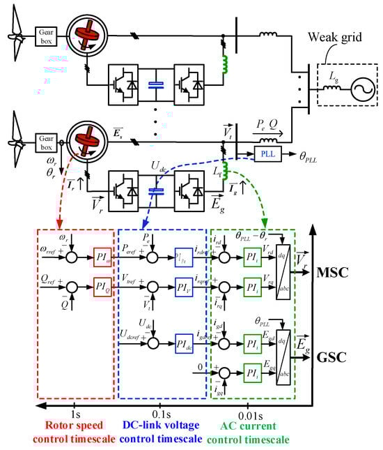
Figure 1.
Multi-timescale dynamics of DFIG connected to weak grid.
2.2. Model of DFIG in DVC Timescale for Power Stability Limits Analysis
Using the terminal voltage phase of DFIG as the reference phase, we make the following assumptions: (1) Regardless of the resistance loss, only the influence of the reactance is taken into account. (2) Regardless of the stator and rotor flux linkage dynamics, define the stator back-EMF as Es = −jXmIr. (3) The response of the current control loop is much faster than that of DVC. Consequently, the current control loop is denoted as an inertia link in the DVC timescale. Based on the above assumptions, the equivalent circuit diagram of DFIG is shown in Figure 2, where Es denotes the stator back-EMF. Ic, Is, Ig represent the current of the gird-side converter, stator current and grid current, respectively. Furthermore, Ut and Ug symbolize the terminal voltage magnitude of DFIG and the infinite bus magnitude.
where the subscripts d and q represent rotating reference frame signal from the d-axis and the q-axis components. s and r signify stator and rotor components, while c and g represent components related to the GSC and grid components, respectively.
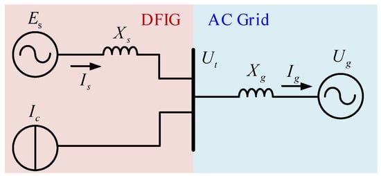
Figure 2.
Equivalent circuit diagram of DFIG system.
Since utq = 0, from Equation (1), it is obtained that
And, according to Pc = Pr = −srPs, there is
From the circuit principle, it is obtained that
The real and imaginary parts on the left and right sides of the equation are equal, and there are
Since utq = 0 and icq = 0, the terminal voltage is
The output active power is
Equation (9) demonstrates that an increase in rotor d-axis current (−ird) will reduce the terminal voltage amplitude, while an increase in rotor q-axis current (irq) will cause the terminal voltage amplitude to increase. Equation (10) indicates that as the rotor d-axis current gradually increases, the active power Pe first increases and then decreases. This is because the rise in −ird not only leads to an increase in its active power but also leads to a reduction in terminal voltage amplitude. As the −ird elevates to a certain value, the rate at which the terminal voltage drops is greater than the rate at which the active power increases. Ultimately, the increase in −ird results in a reduction in active power. Conversely, active power increases with a rise in irq.
2.3. Small Signal Model of DFIG in DVC Timescale for Dynamics Stability Limits Analysis
The model established in the preceding section is based on the assumption that the phase-locked loop precisely follows the phase of the terminal voltage and is suitable for steady-state analysis. However, in actual operation, each control loop within the system exhibits a certain response time. Therefore, control loops, such as phase-locked loops, terminal voltage loops, active power loops, and DC voltage loops, should be considered to establish the small signal model for dynamics stability limit analysis. It needs to be emphasized that the linearization is valid for small perturbations around an operating point and the analysis assumes the system remains within a small neighborhood of equilibrium during disturbances. Additionally, higher-order terms are neglected in the Taylor series expansion.
Figure 3 illustrates the spatial relationship between the synchronous dq reference frame and the PLL-dq reference frame. In the synchronous dq reference frame, the steady-state terminal voltage phase θt0 is defined as zero. F represents vectors such as voltage, current, etc. The relationship between the variables in the synchronous dq frame and the measured values in the PLL reference frame is detailed below:
where θpll represents the angle between the dp-axis and ds-axis. The superscript p represents the component in the PLL coordinate system.
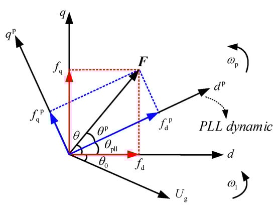
Figure 3.
Spatial relationship between the synchronous dq reference frame and the PLL-dq reference frame.
Linearizing Equations (1)–(10) can obtain
Specific parameters in Equations (15)–(19) are represented in Appendix A.
3. Limit Analysis of Maximum Active Power Output for DFIG Connected to Weak Grid
3.1. Steady State Limit of DFIG Connected to Weak Grid
Utilizing the model of DFIG above, the maximum power of a DFIG system connected to a weak grid under steady state is analyzed. The infinite power supply voltage and grid reactance are set as base values of voltage and impedance, respectively, such as Ug = 1, Xg = 1. And set Xs = 4.071, Xm = 3.9, Xr = 4.056 and sr = −0.2. By combining Equations (9) and (10) and the parameters in Table A1, the relationship between the rotor d/q axis currents, the terminal voltage and active power can be obtained as depicted in Figure 4. From Equation (7), it is obtained that −ird ≤ 0.87. Therefore, the range of the horizontal axis as the coordinate axis in Figure 4a,c is [0, 0.87].
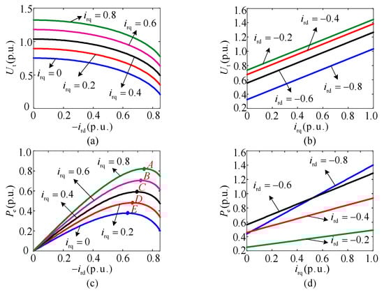
Figure 4.
Rotor d-axis and q-axis current vs. terminal voltage and active power. (a) The curve of terminal voltage in relation to rotor d-axis current; (b) the curve of terminal voltage in relation to rotor q-axis current; (c) the curve of active power in relation to rotor d-axis current; (d) the curve of active power in relation to rotor q-axis current.
Figure 4c presents the curve of active power in relation to the rotor d-axis current. A~E are the points when the output active power achieves its maximum value. Specifically, the coordinates of points A~C are (0.73, 0.88), (0.71, 0.76) and (0.69, 0.63), respectively. It can be seen that when the rotor d-axis current is constant, the larger the rotor q-axis current is, the larger the active power Pe of the DFIG system is, and the larger the rotor d-axis current value, which makes Pe reach the maximum value. Figure 4d shows the curve of active power as a function of the rotor q-axis current. It can be seen that Pe escalates linearly with an increase in irq, and the greater the value of −ird, the faster the rate at which Pe increases with irq.
From the preceding analysis, it has been established that active power and the terminal voltage amplitude are related to the d-axis current and q-axis current of the rotor. Both Pe and Ut are nonlinear functions of ird. When the rotor-side converter is operating in the area of ∂Pe/∂ (−ird) < 0 and there is no dynamic reactive power support, an increase in rotor d-axis currents will cause a decrease in output active power, which in turn will cause the active power control to be unstable.
3.2. Sensitivity-Based Active Power Output Limit Analysis
In order to further study the relationship between Pe, Ut and ird, irq, the characteristics of ∂Ut/∂ (−ird), ∂Ut/∂irq, ∂Pe/∂ (−ird), ∂Pe/∂irq under different operating points are analyzed in this section. From Equations (7) and (9), we derive the conversion relationship between θt0, Ut0 and ird0, irq0:
Analogous to a synchronous generator, the correlation between the output active power and the terminal voltage angle of a DFIG is illustrated in Equation (22). It can be seen that the output active power of a DFIG is proportional to the sine value of the terminal voltage angle and is proportional to θt. Therefore, the active power output Pe can be expressed as follows:
The short-circuit ratio λSCR is generally used to measure the strength of the AC system to which a DC system is connected. At a certain operating point, the λSCR can be approximated as:
It can be seen from Equation (23) that the λSCR is inversely proportional to the line reactance, the active power output of DFIG and the sine value of the terminal voltage angle. Assume the amplitude and phase of the infinite electric network voltage remain unchanged, linearize Equations (7), (9) and (10), and replace id0, iq0 with θt0, Ut0; then, the following can be obtained:
The expressions of ∂Ut/∂ (−ird), ∂Ut/∂irq, ∂Pe/∂ (−ird), ∂Pe/∂irq are:
The sensitivity of the terminal voltage to the rotor d-axis current ∂Ut/∂ (−ird) is proportional to tanθt. Consequently, when θt is large, a minor increase in −ird will cause Ut to a pronounced decrease sharply. The sensitivity of the terminal voltage to the rotor q-axis current ∂Ut/∂irq is constant, and its value is dictated by system parameters. The sensitivity of the active power to the rotor d-axis current ∂Pe/∂ (−ird) is related to θt0, Ut0, and sr. The sensitivity of the active power to the rotor q-axis current ∂Pe/∂irq is inversely proportional to sinθt0.
Figure 5a depicts the curve of ∂Pe/∂ (−ird) and −∂Pe/∂irq as a function of θt0. Figure 5b represents the curve of ∂Pe/∂ (−ird) as a function of λSCR. When λSCR is less than 2, ∂Pe/∂ (−ird) decreases sharply with the decline in λSCR and becomes negative, which restricts the stability limit of DFIG under a weak grid.
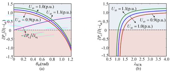
Figure 5.
Curve of ∂Pe/∂ (−ird) as a function of θt0 and λSCR. (a) The curve of ∂Pe/∂ (−ird) and −∂Pe/∂irq as a function of θt0; (b) the curve of ∂Pe/∂ (−ird) as a function of λSCR.
The terminal voltage angle in the case of is defined as the critical terminal voltage angle θtlim:
The steady-state stability limit of output active power is:
From Equation (32), it can be inferred that the active power limit of the DFIG is contingent upon parameters, such as Ut, Ug, Xg and Xs. In the case of constant Ug, Ut and internal parameters of DFIG, the active power limit of the DFIG system is determined by the magnitude of the grid reactance. Thus, the steady-state power limit of the DFIG system is closely related to the grid strength.
The steady-state stability limits of DFIG under varying terminal voltages are established in Table 1. It can be seen that the maximum active power output is 0.83 p.u. in the case of SCR = 1.0 and Ut = 1.0 p.u. Furthermore, the minimum SCR that DFIG can normally operate in is 1.2 in the case of Pe = 1.0 p.u. and Ut = 1.0 p.u.

Table 1.
Stability limit of DFIG at steady state.
4. Stability Limit Analysis of DFIG with Multiple Physical Scenarios
According to the aforementioned small signal model and the parameters outlined in Table A1, the effects of multiple physical scenarios, including grid strength, AVC bandwidth and PLL bandwidth, on the stability limits of DFIG are investigated in this section. First of all, the effect of AVC bandwidth on the stability limit is analyzed. A root locus diagram with increasing AVC bandwidth under different λSCR is shown in Figure 6. It is found that the greater the AVC bandwidth, the higher the stability limit of DFIG becomes. Then, the influence of AVC and PLL dynamics on the stability limit is illustrated in the two cases that follow:
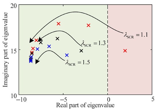
Figure 6.
Root locus diagram with the change in AVC bandwidth.
Case I: Consider the dynamics of the control loops such as phase-locked loop, active power loop, and DC voltage loop, regardless of the dynamics of AVC.
Case II: Consider the dynamics of all control loops including AVC.
Figure 7 depicts the locus of the dominant eigenvalue’s real part as PLL bandwidth increases from 2 Hz to 28 Hz under different SCRs. In extremely weak power grids, as the bandwidth of the PLL increases, the stability limit of DFIG decreases. From Figure 7a in case I, it can be observed that as the bandwidth of PLL changes, the root locus of the dominant eigenvalue is approximately a straight line, and the operation state of the system will not change with the bandwidth of the PLL. Figure 7b in case II illustrates the stability limit of the system changes with the variations in the bandwidth of PLL. In the case of λSCR = 1.19, the system operation state varies from stability to instability with the rise in PLL bandwidth. After a certain degree, the system returns to a stable operating state. Therefore, the dynamic stability limit of the system decreases first and then increases.
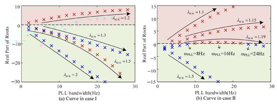
Figure 7.
Curves of real part of eigenvalue as a function of PLL bandwidth. (a) Curves regardless of the dynamics of AVC; (b) curves with all the control loops including AVC.
To sum up, reducing the bandwidth of PLL or increasing the bandwidth of AVC with constant damping can enhance the stability limit of the DFIG system when considering the dynamics of all control loops in case II. However, when the terminal voltage ideally tracks the command value in case I, the system’s stability limit decreases. Meanwhile, the effect of adjusting PLL bandwidth on the stability limit of the DFIG system becomes weaker.
The locus of the eigenvalue’s real part of the DFIG system with varied AVC bandwidth and varied PLL bandwidth is shown in Figure 8 and Figure 9, respectively. The influence trend of the AVC bandwidth on the stability limit is relatively monotonous. The larger the AVC bandwidth is, the higher the system stability limit is. With an increase in AVC bandwidth, it can be found that the maximum active power output for the dynamic stability limit is 0.89 p.u. in the case of SCR = 1.0, and the minimum SCR that DFIG can normally operate in is 1.14 in the case of Pe = 1.0 p.u.
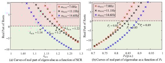
Figure 8.
Effect of AVC bandwidth on stability limit of DFIG.
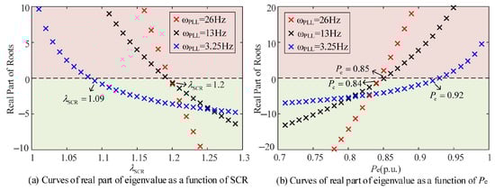
Figure 9.
Effect of PLL bandwidth on stability limit of DFIG.
However, the result becomes complicated when it comes to the variation in PLL bandwidth. When λSCR approximates 1.2 or the output active power approximates 0.85 p.u., the effect of PLL bandwidth on the stability limit of the DFIG system becomes unclear. Combining with the results in Figure 7, Figure 8 and Figure 9, it is suggested that reducing PLL bandwidth with constant damping can enhance the dynamic stability limit of a DFIG when the SCR is smaller than 1.3. When SCR surpasses 1.3, the stability limit can be improved by increasing the bandwidth of PLL with constant damping. After optimal regulation, the maximum active power output for the dynamic stability limit is 0.92 p.u. in the case of SCR = 1.0, and the minimum SCR for normal DFIG operation is 1.09 when Pe = 1.0 p.u.
5. Simulation and Experiment Results
A detailed time-domain model of DFIG connected to a weak grid through long transmission lines is built in MATLAB/Simulink R2021b. The dynamic responses of the active power, terminal voltage, and DC-link voltage of the DFIG with and without considering AVC under varied grid strengths are observed. Moreover, the dynamic responses of the active power, terminal voltage, and DC-link voltage of the DFIG with varied AVC bandwidths and PLL bandwidths are studied.
In Figure 10, it can be observed that the minimum SCR which DFIG can normally operate in is 1.22 when Pe = 1.0 p.u., and AVC dynamics are not considered. However, as considering the dynamics of all control loops on the DVC timescale, the minimum SCR which DFIG can normally operate in is 1.20, which is smaller than the former, as depicted in Figure 11. Thus, it is revealed that the stability limit of DFIG becomes larger when considering AVC dynamics than without considering them, which agrees with the results derived from Figure 7. Figure 10 shows that it depicts response waveforms without considering AVC dynamics, contrasting stable operation (λSCR = 1.22) with instability onset (λSCR = 1.20), while Figure 11 presents waveforms that incorporate AVC dynamics, indicating enhanced stability limits consistent with the root locus analysis in Section 4.
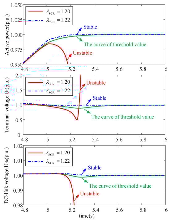
Figure 10.
Response waveforms without considering AVC.
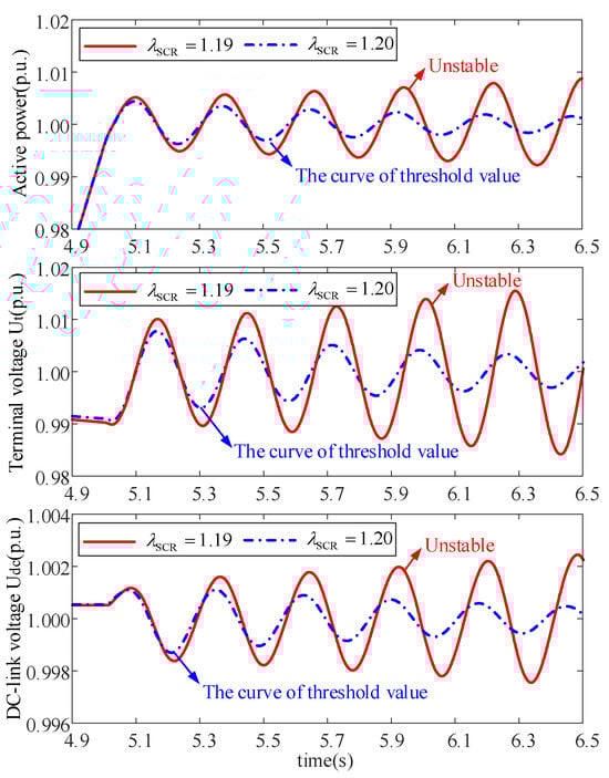
Figure 11.
Response waveforms considering AVC.
The active power output of DFIG is slowly increased to reach the stability limit under varying AVC bandwidths and different PLL bandwidths, respectively, under the condition of SCR = 1.2. Figure 12 and Figure 13 illustrate these findings. The investigation reveals that the active power limit is 1.0 p.u. as AVC bandwidth is 14.6 Hz larger than the active power limit with ωAVC = 7 Hz or 11.1 Hz. Furthermore, the active power limit is set at 1.0 p.u. when the PLL bandwidth is 3.25 Hz larger than the active power limit with ωPLL = 13 Hz or 26 Hz. Therefore, it is revealed that increasing the bandwidth of AVC or decreasing the bandwidth of PLL can enhance the dynamic stability limit of DFIG with SCR = 1.2. This observation aligns with the findings presented in Figure 8 and Figure 9.
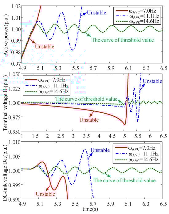
Figure 12.
Stability limit analysis with varied AVC bandwidths.
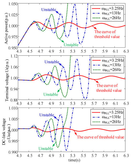
Figure 13.
Stability limit analysis with varied PLL bandwidths.
6. Experiment Results
As depicted in Figure 14, the experimental platform provides empirical confirmation of the theoretical analysis of a DFIG connected to a weak grid. This verification is achieved through the use of an actual 6 kW Doubly Fed Induction Generator system. Real-time control of both the rotor-side converter and grid-side converter is executed on a high-performance national instrument platform: ultra-low latency processing for critical high-speed switching tasks, including PWM generation and protection algorithms, is handled by an NI FlexRIO FPGA board (PXIe-7868R), while higher-level supervisory control functions operate on an NI PXIe-1071 real-time controller housed in a PXIe chassis. By incorporating variable grid impedance between the point of common coupling of the DFIG and the primary laboratory supply, controlled weak grid scenarios are accurately emulated. This allows for a systematic reduction in the grid strength, quantified by the short-circuit ratio, effectively simulating low-inertia conditions to rigorously test system stability and dynamic performance against theoretical predictions. In the experiments, λSCR values were set by adjusting the grid impedance Xg to vary Ug × Ug/(Xg × Pe) according to Equation (23).
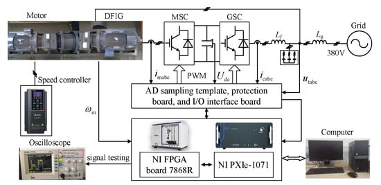
Figure 14.
Experimental platform for DFIG connected to weak grid.
Figure 15 presents the experimental results, illustrating the system behavior with AVC dynamics considered. Case (a) (λSCR = 1.22) exhibits stable operation, characterized by well-damped oscillations converging to steady-state values in active power and DC-link voltage. Conversely, Case (b) (λSCR = 1.20) shows clear instability, evidenced by sustained and growing oscillations in both Pe and Udc. This confirms the simulation results shown in Figure 11 and validates that with AVC dynamics, the system goes unstable for λSCR ≈ 1.20 or below. Figure 16 shows the results without AVC dynamics. Case (a) (λSCR = 1.20) remains stable, while Case (b) (λSCR = 1.19) becomes unstable. This experimentally confirms the simulation results in Figure 10, demonstrating that excluding AVC dynamics increases the minimum stable SCR for Pe = 1.0 p.u. from 1.20 with AVC to 1.22 without AVC, thus proving AVC dynamics enhance the assessed stability limit under weak grid conditions.
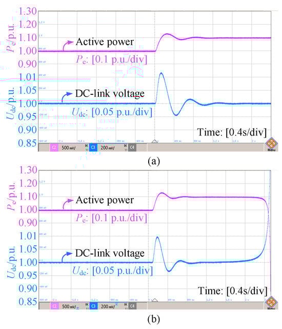
Figure 15.
Experiment results considering AVC. (a) In the case of λSCR = 1.22; (b) in the case of λSCR = 1.20.
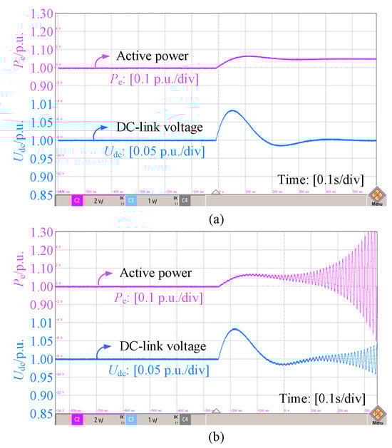
Figure 16.
Experiment results without considering AVC. (a) In the case of λSCR = 1.2; (b) in the case of λSCR = 1.19.
Figure 17 experimentally investigates the effects of varying AVC bandwidth under a fixed weak grid with λSCR = 1.2. Case (a) (ωAVC = 14.5 Hz) maintains stable operation at the target Pe = 1.0 p.u., with minimal Udc deviation. Cases (b) (ωAVC = 11 Hz) and (c) (ωAVC = 7 Hz), nevertheless, display instability at active power levels substantially below 1.0 p.u. This directly corroborates the simulation in Figure 12, substantiating that a higher AVC bandwidth increases the dynamic stability limit. Figure 18 examines PLL bandwidth effects under the same weak grid. Case (a) (ωPLL = 3 Hz) sustains stability at Pe = 1.0 p.u. Cases (b) (ωPLL = 13 Hz) and (c) (ωPLL = 26 Hz) become unstable, with Udc exhibiting significant oscillations. This affirms the simulation results depicted in Figure 13, demonstrating that reducing PLL bandwidth enhances the stability limit under this specific weak grid condition with λSCR = 1.2. The consistent response patterns between Pe and Udc across all cases provide strong experimental validation for the theoretical bandwidth dependency analysis.
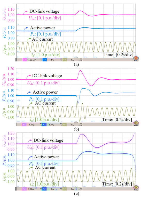
Figure 17.
Experiment results with varied AVC bandwidths. (a) ωAVC = 14.5 Hz; (b) ωAVC = 11 Hz; (c) ωAVC = 7 Hz.
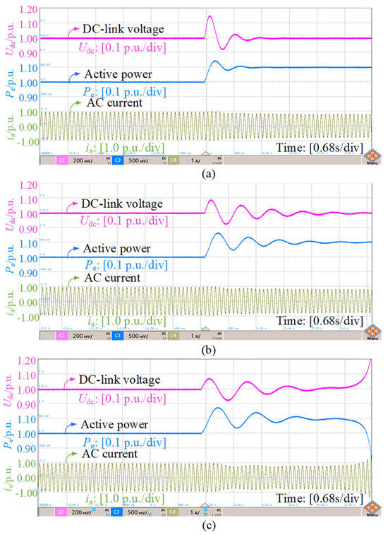
Figure 18.
Experiment results with varied PLL bandwidths. (a) ωPLL = 3 Hz; (b) ωPLL = 13 Hz; (c) ωPLL = 26 Hz.
The experimental results emphasize Udc and Pe as primary stability indicators since these directly reflect the DC-link voltage control timescale dynamics that are the focus of this study, while AC current waveforms in Figure 17 and Figure 18 serve as secondary confirmation of PLL/AVC bandwidth effects. In the captions of Figure 15, Figure 16, Figure 17 and Figure 18, we specify which specific stability phenomenon each experimental result verifies, with direct equation references. These changes create clearer correspondence between the multi-timescale theoretical analysis and selective but targeted experimental demonstrations.
7. Conclusions
This study investigates the stability limits of weak-grid-connected DFIG in a DC-link voltage control timescale. The steady-state model and small signal analysis model of DFIG under the weak grid were developed. The constraint factors of the active power limit in steady state and the impact of control loop coupling on the dynamic stability limit of DFIG are analyzed. The stability limits presented here are derived from our specific experimental and simulation setup. However, the proposed methodology, including sensitivity analysis of ∂Pe/∂ (−ird) and eigenvalue-based dynamics assessment, offers a generalizable framework to predict stability limits in other scenarios by adapting parameters such as grid reactance or control loop bandwidths. The conclusions are as follows:
(1) The steady stability boundary of DFIG is defined by the partial derivative of active power with respect to d-axis rotor current ∂Pe/∂ (−ird). As ∂Pe/∂ (−ird) becomes zero, the system reaches the steady stability limit in the DVC timescale.
(2) The dynamics stability boundary of DFIG is strongly influenced by AVC dynamics under weak grid conditions. The stability limit of DFIG becomes larger when considering AVC dynamics as opposed to without AVC dynamics. Furthermore, increasing the bandwidth of AVC enhances the dynamics stability limit of DFIG.
(3) Decreasing PLL bandwidth with constant damping can enhance the dynamic stability limit of DFIG as SCR is smaller than 1.3, and the stability limit can be improved by raising PLL bandwidth with constant damping when SCR is greater than 1.3.
(4) Through optimized regulation, the max active power output of DFIG for the dynamic stability limit can reach 0.92 p.u. (with SCR = 1); correspondingly, the minimum SCR in which DFIG can normally operate for the dynamic stability limit is 1.09 (with Pe = 1.0 p.u.) in the DVC timescale. While the numerical thresholds (SCR 1.09 for Pe = 1.0 p.u.) are system-dependent, the trends and critical factors maintain broader relevance for weak-grid-connected DFIG systems.
Author Contributions
Methodology, K.J.; software, K.J.; validation, L.L. and Z.H.; formal analysis, L.L.; investigation, D.L.; resources, K.J.; data curation, L.L.; writing—original draft, Z.H.; writing—review and editing, K.J.; supervision, D.L.; project administration, L.L.; funding acquisition, K.J. All authors have read and agreed to the published version of the manuscript.
Funding
This work was supported by the Science and Technology Project of Hubei Power Grid Corporation (52153223001R).
Data Availability Statement
The data that support the findings of this study are available on request from the corresponding author. The data are not publicly available due to privacy or ethical restrictions.
Acknowledgments
We thank the editor and the anonymous reviewers for their constructive comments that helped to improve our work.
Conflicts of Interest
The authors declare no conflicts of interest.
Abbreviations
| Pe | Active power output of DFIG |
| Es | The stator back-EMF |
| Ut | Terminal voltage magnitude of DFIG |
| Ug | Infinite bus voltage magnitude |
| Ic | current of the gird side converter |
| Is, Ir | Stator current and rotor current |
| θt | The phase theta of the grid terminal voltage |
| θpll | The angle between dp-axis and ds-axis |
| Udc | DC-link voltage |
| C | DC-link capacitance |
| Xg | Transmission Line impedance |
| Xs, Xr, Xm | The equivalent reactance of stator winding and rotor winding and their mutual inductance |
| sr | Slip ratio |
| Sac | Short-circuit capacity of the AC grid |
| , | Proportion coefficient and integral coefficient of DC-link voltage controller |
| , | Proportion coefficient and integral coefficient of PLL |
| , | Proportion coefficient and integral coefficient of terminal voltage controller |
| , | Proportion coefficient and integral coefficient of active power controller |
| ωAVC | The bandwidth of ac voltage control loop |
| ωPLL | The bandwidth of PLL |
| Superscript: | |
| p | Phase-locked loop coordinate system |
| s | Ideal synchronous rotating coordinate system |
| Subscripts: | |
| ref | Reference value |
| d, q | Rotating reference frame signal d-axis and q-axis components |
| s, r | Stator and rotor components |
| c, g | GSC and grid components |
| 0 | Initial value in steady operating point |
Appendix A
Parameters from K1 to K13 are shown as follows,
Table A1.
DFIG parameters for simulation.
Table A1.
DFIG parameters for simulation.
| Parameters | Values |
|---|---|
| Rated power | 2.0 MW |
| Rated voltage | 690 V |
| DC voltage | 1200 V |
| 1.6, 240 | |
| , | 1100 |
| , | 3200 |
| , | 60, 1400 |
References
- Guo, X.; Yuan, X.; Zhu, D.; Zou, X.; Hu, J. Evaluation and Optimization of DFIG-Based WTs for Constant Inertia as Synchronous Generators. IEEE Trans. Power Electron. 2024, 39, 10453–10464. [Google Scholar] [CrossRef]
- Latif, M.; Ambreen, H.; Hassan, F.; Imran, M. Computationally Efficient Reduced Order Modeling of DFIG-Based Wind Turbines: A Novel Frequency-Weighted and Limited Model Reduction Approach with Error Bounds. IEEE Access 2024, 12, 54299–54315. [Google Scholar] [CrossRef]
- Buragohain, U.; Mir, A.S.; Senroy, N. Transient Stability Assessment of a DFIG-WTG System Using Trajectory Sensitivity Analysis. IEEE Trans. Power Syst. 2024, 39, 5818–5828. [Google Scholar] [CrossRef]
- Guo, C.; Yang, S.; Liu, W.; Zhao, C.; Hu, J. Small-Signal Stability Enhancement Approach for VSC-HVDC System Under Weak AC Grid Conditions Based on Single-Input Single-Output Transfer Function Model. IEEE Trans. Power Deliv. 2021, 36, 1313–1323. [Google Scholar] [CrossRef]
- Sun, C.; Yang, Y.; Zhu, D.; Zou, X.; Kang, Y. Systematic Controller Design for DFIG-Based Wind Turbines to Enhance Synchronous Stability During Weak Grid Fault. In Proceedings of the 2023 IEEE/IAS Industrial and Commercial Power System Asia (I&CPS Asia), Chongqing, China, 7–9 July 2023; pp. 1587–1592. [Google Scholar]
- Du, W.; Wang, Y.; Wang, H.; Xiao, X.; Wang, X.; Xie, X. Analytical Examination on the Amplifying Effect of Weak Grid Connection for the DFIGs to Induce Torsional Sub-Synchronous Oscillations. IEEE Trans. Power Deliv. 2020, 35, 1928–1938. [Google Scholar] [CrossRef]
- Sun, P.; Yao, J.; Liu, R.; Pei, J.; Zhang, H.; Liu, Y. Virtual Capacitance Control for Improving Dynamic Stability of the DFIG-Based Wind Turbines During a Symmetrical Fault in a Weak AC Grid. IEEE Trans. Ind. Electron. 2021, 68, 333–346. [Google Scholar] [CrossRef]
- Nair, A.; Kamalasadan, S.; Geis-Schroer, J.; Patel, S.; Smith, M. An Investigation of Grid Stability and a New Design of Adaptive Phase-Locked Loop for Wind-Integrated Weak Power Grid. IEEE Trans. Ind. Appl. 2022, 58, 5871–5884. [Google Scholar] [CrossRef]
- Li, Z.; Xu, H.; Wang, Z.; Yan, Q. Stability Assessment and Enhanced Control of DFIG-Based WTs During Weak AC Grid. IEEE Access 2022, 10, 41371–41380. [Google Scholar] [CrossRef]
- Guo, X.; Zhu, D.; Zou, X.; Yang, Y.; Kang, Y.; Tang, W.; Peng, L. Analysis and Enhancement of Active Power Transfer Capability for DFIG-Based WTs in Very Weak Grid. IEEE J. Emerg. Sel. Top. Power Electron. 2022, 10, 3895–3906. [Google Scholar] [CrossRef]
- Ying, J. Impact of Inertia Control on the Structural Loads of DFIG-based Wind Turbine Connected to Weak Grid. In Proceedings of the 2020 12th IEEE PES Asia-Pacific Power and Energy Engineering Conference (APPEEC), Nanjing, China, 20–23 September 2020; pp. 1–5. [Google Scholar]
- Huang, Y.; Wang, L.; Zhang, S.; Wang, D.; Deng, X.; Zhu, G. Impacts of Phase-Locked Loop Dynamic on the Stability of DC-Link Voltage Control in Voltage Source Converter Integrated to Weak Grid. IEEE J. Emerg. Sel. Top. Circuits Syst. 2022, 12, 48–58. [Google Scholar] [CrossRef]
- Hu, J.; Yuan, H.; Yuan, X. Modeling of DFIG-Based WTs for Small-Signal Stability Analysis in DVC Timescale in Power Elec-tronized Power Systems. IEEE Trans. Energy Convers. 2017, 32, 1151–1165. [Google Scholar] [CrossRef]
- Hu, J.; Huang, Y.; Wang, D.; Yuan, H.; Yuan, X. Modeling of Grid-Connected DFIG-Based Wind Turbines for DC-Link Voltage Stability Analysis. IEEE Trans. Sustain. Energy 2015, 6, 1325–1336. [Google Scholar] [CrossRef]
- Morshed, M.J.; Fekih, A. A Coordinated Controller Design for DFIG-Based Multi-Machine Power Systems. IEEE Syst. J. 2019, 13, 3211–3222. [Google Scholar] [CrossRef]
- Shanmugam, R.; Sakthivel, D.K.; Ramaiah, A.N.; Ramalingam, S. Nonlinear Control Strategy for DC-Link Voltage Control in a DFIG of WECS During 3φ Grid Faults. IEEE Trans. Ind. Electron. 2024, 71, 12468–12475. [Google Scholar] [CrossRef]
- Shen, Y.; Ma, J.; Wang, L.; Phadke, A.G. Study on DFIG Dissipation Energy Model and Low-Frequency Oscillation Mechanism Considering the Effect of PLL. IEEE Trans. Power Electron. 2020, 35, 3348–3364. [Google Scholar] [CrossRef]
- Liu, J.; Yao, W.; Wen, J.; Fang, J.; Jiang, L.; He, H.; Cheng, S. Impact of Power Grid Strength and PLL Parameters on Stability of Grid-Connected DFIG Wind Farm. IEEE Trans. Sustain. Energy 2020, 11, 545–557. [Google Scholar] [CrossRef]
- Guo, X.; Zou, X.; Jiang, C.; Zhu, D.; Yang, Y.; Peng, L.; Lin, X. Active Power Limit for DFIG-Based Wind Turbine under Weak Grid. In Proceedings of the 2019 IEEE Energy Conversion Congress and Exposition (ECCE), Baltimore, MD, USA, 29 September–3 October 2019; pp. 968–973. [Google Scholar]
- Du, W.; Dong, W.; Wang, H.F. Small-Signal Stability Limit of a Grid-Connected PMSG Wind Farm Dominated by the Dynamics of PLLs. IEEE Trans. Power Syst. 2020, 35, 2093–2107. [Google Scholar] [CrossRef]
- Peng, Q.; Fang, J.; Yang, Y.; Liu, T.; Blaabjerg, F. Maximum Virtual Inertia From DC-Link Capacitors Considering System Stability at Voltage Control Timescale. IEEE J. Emerg. Sel. Top. Circuits Syst. 2021, 11, 79–89. [Google Scholar] [CrossRef]
- Ma, Y.; Zhu, D.; Hu, J.; Liu, D.; Ji, X.; Zou, X.; Kang, Y. Reduced-Order Modeling and Transient Stability Analysis of Grid-Connected VSC in DC-Link Voltage Control Timescale. IEEE J. Emerg. Sel. Top. Power Electron. 2024, 12, 2981–2993. [Google Scholar] [CrossRef]
Disclaimer/Publisher’s Note: The statements, opinions and data contained in all publications are solely those of the individual author(s) and contributor(s) and not of MDPI and/or the editor(s). MDPI and/or the editor(s) disclaim responsibility for any injury to people or property resulting from any ideas, methods, instructions or products referred to in the content. |
© 2025 by the authors. Licensee MDPI, Basel, Switzerland. This article is an open access article distributed under the terms and conditions of the Creative Commons Attribution (CC BY) license (https://creativecommons.org/licenses/by/4.0/).