Coordinated Control of Grid-Forming Inverters for Adaptive Harmonic Mitigation and Dynamic Overcurrent Control

Abstract

This paper proposes a coordinated control strategy for grid-forming inverters (GFMs) to address two critical challenges in evolving power systems. These are the active harmonic mitigation under nonlinear loading conditions and dynamic overcurrent control during grid disturbances. The proposed framework integrates a shunt active filter (SAF) mechanism within the GFM control structure to achieve a real-time suppression of harmonic distortions from the inverter and grid currents. In parallel, a virtual impedance-based dynamic current limiting strategy is incorporated to constrain fault current magnitudes, ensuring the protection of power electronic components and maintaining system stability. The SAF operates in a current-injection mode aligned with harmonic components, derived via instantaneous reference frame transformations and selective harmonic extraction. The virtual impedance control (VIC) dynamically modulates the inverter’s output impedance profile based on grid conditions, enabling adaptive response during fault transients to limit overcurrent stress. A detailed analysis is performed for the coordinated control of the grid-forming inverter. Supported by simulations and analytical methods, the approach ensures system stability while addressing overcurrent limitations and active harmonic filtering under nonlinear load conditions. This establishes a viable solution for the next-generation inverter-dominated power systems where reliability, power quality, and fault resilience are paramount.

1. Introduction

The ongoing evolution of power systems toward decentralized architectures and renewable energy integration fundamentally transforms grid dynamics. Central to this transformation is the development of GFMs, which, unlike traditional grid-following converters, possess the intrinsic ability to establish voltage and frequency references. Emulating the behavior of synchronous machines through advanced control paradigms, GFMs are poised to become the backbone of inverter-dominated power systems. They contribute decisively to frequency regulation, voltage stability, and islanding capabilities in weak or fragmented grids [1,2,3,4].

However, as GFMs become central to future power systems, they must address power quality issues that were traditionally managed by other grid elements, most notably, harmonic distortions introduced by nonlinear loads. This challenge becomes more insistent in inverter-dominated networks, where traditional passive components are either downsized or absent. Historically, such harmonic distortions were mitigated using passive filtering techniques. These filters, although simple, suffer from poor adaptability to dynamic grid conditions, resonance risks, and detuning effects, limiting their effectiveness in modern power systems [5,6]. To overcome these drawbacks, active filtering strategies emerged, using voltage source converters operating in current control modes. These active filters inject counter-harmonic currents to mitigate distortions and adapt more effectively to system changes. Among various active filter topologies, SAFs have gained prominence due to their ability to integrate seamlessly with distributed generation systems and their high control flexibility [7,8,9,10].

Despite advancements in active filtering, modern power systems face new challenges beyond harmonic suppression, particularly in inverter-dominated grids where GFMs must ensure both power quality and protection. Under fault conditions, fault currents may exceed the safe operating limits of power semiconductor devices, risking permanent damage [11]. Traditional protection techniques are deficient in GFM-controlled systems where inertia and short-circuit capability are low.

Current studies have proposed several overcurrent control strategies for grid-connected inverters to address the limitations of traditional protection mechanisms in low-inertia systems. Approaches such as instantaneous current limiting, saturation-based control, and dynamic reference scaling have been explored to constrain fault currents within device ratings while preserving system stability [12,13]. However, many of these methods either compromise voltage regulation or introduce undesired dynamic interactions with the grid. VIC has gained attention as a promising solution to enhance fault ride-through capability without undermining the grid-forming role. By dynamically shaping the inverter output impedance in response to fault conditions, VIC enables current limiting, improved voltage support, and enhanced damping of resonances. Moreover, VIC can be seamlessly integrated into GFM control frameworks without disrupting synchronization or droop characteristics. It is well-suited for inverter-dominated grids where precise power sharing, harmonic rejection, and protection must coexist. Recent work on impedance matching in power amplifiers using non-adoptive-based circuits shows how adjusting impedance in real time can improve power transfer and system stability across changing conditions [14,15]. This supports the use of virtual impedance control in GFM inverters, where adaptive impedance helps limit fault currents and maintain stable operation during grid disturbances.

This paper identifies a critical knowledge gap in the absence of integrated control strategies that unify harmonic mitigation and fault current limitation in GFMs. While SAFs are well-studied for harmonic compensation, and virtual impedance methods have been explored for fault current limitation, there is little research that investigates their coordinated operation within a single GFM framework. Addressing this integration is essential for developing resilient, multifunctional inverters suited for modern power grids. This is especially significant considering that institutions like the North American Electric Reliability Corporation (NERC) now emphasize the necessity of such advanced support functionalities [16].

Motivated by these challenges, this paper proposes a unified control strategy that integrates SAF for harmonic mitigation with VIC for dynamic overcurrent limitation within a grid-forming inverter framework. The proposed dual-function architecture enhances both power quality and fault resilience, enabling the inverter to operate reliably under nonlinear loading and fault conditions [13,17,18,19]. Crucially, the coordination between SAF and virtual impedance functions is carefully synthesized to prevent dynamic interference, ensuring stable operation and preserving the fundamental grid-forming objectives such as voltage regulation, synchronization, and power sharing.

To validate the proposed dual-function control scheme and demonstrate its practical feasibility, a detailed system-level model is developed. Figure 1 illustrates the integrated control architecture of the proposed system, comprising a GFM, a nonlinear load, a synchronous generator, and a SAF. The GFM inverter is modeled as a voltage source with nested voltage and current controllers. The voltage controller generates a reference current to maintain voltage regulation, while the current controller ensures precise current tracking through PWM switching [20,21]. An LC filter smooths high-frequency components at the point of common coupling (PCC). To limit fault currents, a VIC scheme emulates dynamic output impedance by injecting virtual voltage drops derived from dq-frame current components [22]. Simultaneously, the SAF mitigates load-induced harmonics by injecting compensating currents using a PI-regulated DC-link controller and a harmonic current control loop. The synchronous generator contributes to real and reactive power sharing at the PCC. Power flow interactions between the inverter (Pi, Qi), SAF (Pf, Qf), and grid (Pg, Qg) are also depicted.

The novel aspects of this work can be stated as follows: (i) The proposed system introduces a unified control strategy that seamlessly coordinates GFM control, virtual impedance, and active harmonic filtering. (ii)This comprehensive framework enhances grid stability, improves power quality, and strengthens fault ride-through capability. (iii) Extensive simulation studies demonstrate the control scheme’s effectiveness in mitigating harmonic distortion and dynamically limiting overcurrent during fault events, thereby validating its suitability for modern resilient power systems.

The paper is organized as follows. Section 2 presents the modeling of virtual impedance within the integrated grid-forming inverter system, detailing how it contributes to fault current limitation and system robustness. Section 3 describes the grid dynamics and the control strategy of the SAF for harmonic mitigation. Section 4 provides simulation results and discussions that validate the effectiveness of the proposed unified control approach under various operating conditions, including both steady-state and fault scenarios. Finally, Section 5 concludes the paper by summarizing the key contributions and findings.

2. Modeling of Virtual Impedance in the Integrated System

A GFM regulates voltage and frequency autonomously, behaving as a controlled voltage source behind an impedance. Unlike traditional synchronous generators, inverters require active control strategies to prevent excessive fault currents. One possible way to limit the fault current is the saturation of the current reference in the inner current control loop of the GFM. Saturating the current reference moves the converter from voltage to current regulation mode and introduces several challenges. When the inverter shifts from voltage regulation to current regulation mode, it can no longer maintain the grid voltage at the desired reference, potentially causing voltage deviations and affecting power quality [23]. This transition may also lead to instability if not carefully managed, as abrupt changes in control logic can induce oscillations. Additionally, the inverter’s ability to provide reactive power support during faults is compromised, reducing its fault ride-through capability.

Another way to control the current is the dynamic VIC method, which is implemented in this paper. This method aims to modify the inverter output voltage magnitude when the current exceeds a threshold value. This method introduces a virtual impedance that dynamically adjusts based on the output current. By continuously monitoring the output current and adjusting the virtual impedance accordingly, this method provides a robust mechanism for overcurrent protection in GFMs [13]. The following equations define how the inverter output voltage reference is modified through virtual impedance:

$$V_{id}^{*}=V_{id}^{*\prime }-(R_{VI}{i}_{id}-{jX}_{VI}{i}_{iq})$$

(1)

$$V_{iq}^{*}=V_{iq}^{*\prime }-(R_{VI}{i}_{iq}+{jX}_{VI}{i}_{id})$$

(2)

$$\mathrm{Where} X_{VI}=\left\{\begin{array}{c}{k}_{P_{R\_VI}}\times {\sigma }_{\frac{X}{R}}\times ∆I ;if ∆I>0\\ 0; if ∆I \le 0\end{array}\right.\mathrm{and} R_{VI}= {\displaystyle \frac{X_{VI}}{{\sigma }_{\frac{x}{R}}}}$$

(3)

where $V_{id}^{*}$ and $V_{iq}^{*}$ are the modified inverter output voltage references in the dq frame. $V_{id}^{*\prime }$ and $V_{iq}^{*\prime }$ are the initial voltage references from the outer voltage loop, $i_{idq}$ is the inverter current, and $Z_{VI}=R_{VI}+j{X}_{VI}$ is the virtual impedance applied. The virtual impedance components are dynamically adjusted based on the current deviation ΔI, defined as the difference between the actual current and its reference or nominal value. The expressions for the virtual reactance and resistance are given in Equation (3). $k_{P_{R\_VI}}$ is a proportional gain that governs how aggressively the virtual impedance is adjusted in response to the current deviation. It controls the magnitude of the dynamic virtual reactance and thus influences the inverter’s fault current limiting behavior and voltage support capability during transient events. ${\sigma }_{X/R}$ defines the desired ratio of virtual reactance to resistance for the virtual impedance. It shapes the angle of the virtual impedance vector, determining the phase relationship between voltage drop and current. Together, $k_{P_{R\_VI}}$ and ${\sigma }_{X/R}$ enable flexible tuning of the inverter’s dynamic response, enhancing both stability and fault ride-through capability. The conditional nature of X_VI ensures that the virtual impedance is only activated during overcurrent events (ΔI > 0), thus preserving nominal operation under normal conditions. This mechanism plays a key role in shaping inverter behavior under abnormal grid conditions by limiting fault currents and reducing voltage distortion. It supports the coordinated control strategy by offering a tunable link between voltage and current loops, thereby enhancing overall system stability and safety.

3. Grid Dynamics and Control of Shunt Active Filter

An active filter generates a compensating current that cancels out the harmonics from the inverter and grid currents due to the distorted load current. The load current can be expressed in the fundamental and harmonic components as (4). The inverter with the active filter modifies its output current at the PCC to include the compensating current.

$$i_L=i_{L1}+i_{Ln}$$

(4)

$$i_f\left(t\right)=-i_{Ln}\left(t\right)$$

(5)

The filter current i_f is derived from the harmonic compensating current, which itself is a function of the voltage at the PCC and the load current. Thus, the SAF analyzes the voltage and current at the PCC to determine the unwanted harmonic components introduced by nonlinear loads. Based on this analysis, it generates a compensation current to cancel those harmonics [24,25]. Figure 2 illustrates the SAF control in detail. The load current i_L is measured and transformed into the dq reference frame. High-pass filters (hpf) isolate the harmonic components in the d and q axes. These harmonic components form the basis for the reference current that the SAF must inject to cancel the undesirable harmonics. Specifically, the q-axis reference current is set directly as i_q,ref. In contrast, the d-axis reference current includes an additional term I_dc, which is generated through a DC-link voltage control loop. This component ensures that the inverter supplies enough real power to maintain the DC-link voltage, compensating for system losses. Simultaneously, the actual SAF current i_f is subtracted from the Idq_f to generate control signals. These signals guide the inverter to produce output currents that effectively cancel the harmonics in the load current while maintaining a stable DC-link voltage.

3.1. Coordinated Control of the Proposed System

The proposed system integrates a GFM, an SG, a nonlinear load, and a SAF at the PCC. Coordinated control among these components ensures voltage and frequency stability, harmonic mitigation, and protection against overcurrent events.

The control objective is twofold: (1) To regulate voltage and frequency at the PCC through active power sharing between the SG and GFM, (2) To ensure the injected current from the source remains sinusoidal and in phase with the fundamental component of the load current, leaving harmonic and reactive compensation to the SAF. The nonlinear load draws both fundamental and harmonic currents. The GFM and SG are designed to supply only the fundamental active power, while the SAF compensates for harmonic and reactive components. The total load current can be decomposed as follows:

$$i_L=i_{GFM}+i_{grid}+i_{filt}$$

(6)

$$i_L\left(t\right)=I_{1}sin\left(\omega t+{\varnothing }_1\right)+{\sum }_{n=3,5,\dots }^{\infty }{I}_{n}sin\left(n\omega t+{\varnothing }_n\right)$$

(7)

The load’s power can be computed as the product of the current flowing through the load and the voltage across the load (equal to the voltage at the PCC).

$$P_L\left(t\right)=V_S\left(t\right)\times i_L\left(t\right)$$

(8)

$$P_L\left(t\right)=V_m{I}_1{sin}^2\left(\omega t\right)cos\left({\mathrm{\varnothing }}_1\right)+{\displaystyle \frac{V_m{I}_1}{2}}sin\left(2\omega t\right)sin\left({\mathrm{\varnothing }}_1\right)+V_{m}sin\left(\omega t\right){\sum }_{n=3,5,\dots }^{\mathrm{\infty }}{I}_{n}sin\left(n\omega t+{\mathrm{\varnothing }}_n\right)$$

(9)

$$P_L\left(t\right)=P_F\left(t\right)+P_Q\left(t\right)+P_n\left(t\right)$$

(10)

${\mathrm{P}}_{\mathrm{F}}\left(\mathrm{t}\right), {\mathrm{P}}_{\mathrm{Q}}\left(\mathrm{t}\right) \mathrm{a}\mathrm{n}\mathrm{d} {\mathrm{P}}_{\mathrm{n}}\left(\mathrm{t}\right)$ Represent the fundamental, reactive, and harmonic power drawn by the load, respectively. The source power must match the fundamental component to achieve a unity power factor.

$$V_S\left(t\right)\times i_S\left(t\right)=P_F\left(t\right)=V_m{I}_1{sin}^2\left(\omega t\right)cos\left({\varnothing }_1\right)$$

(11)

$$i_S\left(t\right)={\displaystyle \frac{V_m{I}_1{sin}^2\left(\omega t\right)cos\left({\varnothing }_1\right)}{V_S\left(t\right)}}=I_{m}sin\left(\omega t\right) \hspace{1em} \left\{I_m=I_{1}cos\left({\varnothing }_1\right)\right\}$$

(12)

The SAF is tasked with compensating ${\mathrm{P}}_{\mathrm{Q}}\left(\mathrm{t}\right)$ and ${\mathrm{P}}_{\mathrm{n}}\left(\mathrm{t}\right)$, thereby ensuring that $i_S\left(t\right)$ remains purely sinusoidal and in phase with the PCC voltage.

Equation (13) defines the power balance at the PCC. The power generated by these sources must collectively supply the load demand, the losses, and the power dissipated in the filter. This power equilibrium can be expressed as follows:

$$P_{SG}+P_{GFM}=P_{load }+P_{loss}+P_{filter}$$

(13)

$$V_{pcc}{I}_{SG}\mathit{cos}{\varnothing }_{SG}+V_{pcc}{I}_{GFM }\mathit{cos}{\varnothing }_{GFM}=V_{pcc}\left(I_{load }-I_{filt}\right)\mathit{cos}{\varnothing }_{load}+P_{loss}$$

(14)

$$V_{PCC}=V_{GFM}-Z_{line}\left(I_{load}-I_{filt}\right)$$

(15)

The frequency dynamics of the system are modeled based on the mismatch between the total active power supplied by the sources and the power demanded.

$${\omega }_{pcc}={\displaystyle \frac{\left[\begin{array}{c}{V}_{pcc}{I}_{SG}\mathit{cos}{\varnothing }_{SG}+V_{pcc}{I}_{GFM }\mathit{cos}{\varnothing }_{GFM}\\ -V_{pcc}\left(I_{load }-I_{filt}\right)\mathit{cos}{\varnothing }_{load}-P_{loss}\end{array}\right]}{J_{sys}}}$$

(16)

J_sys is the system’s combined inertia, and this expression highlights how active power imbalances drive frequency deviations.

The proposed coordinated control ensures sFI voltage and frequency regulation by enabling the SG and GFM to supply only fundamental active power, while the shunt filter compensates for harmonic and reactive components. A power equilibrium model, incorporating line impedance and system inertia, governs dynamic interactions at the PCC. This strategy ensures effective power sharing, harmonic mitigation, and frequency stability under nonlinear loading conditions.

3.2. Design Parameters for the System Under Study

The harmonic components of the load current, which directly impact the SAF’s rating and need to be compensated, are determined from the Fast Fourier Transform analysis of the load current. The following computations are performed for a 1000 kW rated load. Equation (17) provides the apparent power S, which is used to calculate the output current at the load.

$$\begin{gathered} \mathrm{S}={\mathrm{V}}_L\times {\mathrm{i}}_L={\displaystyle \frac{3\sqrt{6}}{\mathsf{\pi }}}{\mathrm{V}}_{\mathrm{p}\mathrm{c}\mathrm{c}}\times {\mathrm{i}}_L \\ 1000 \mathrm{k}\mathrm{W}={\displaystyle \frac{3\sqrt{6}}{\mathsf{\pi }}}\times {\displaystyle \frac{600}{\sqrt{3}}}\times {\mathrm{i}}_L \to {\mathrm{i}}_L=1233.68 \mathrm{A} \end{gathered}$$

(17)

Equation (18) gives the input per-phase current for a three-phase full-wave rectifier working as a nonlinear load. The harmonic current is calculated by (19), which helps to find the rating of the SAF (S_SAF).

$${\mathrm{i}}_{L\_ph}={\displaystyle \frac{i_L}{\sqrt{3}}}=712.28 \mathrm{A}$$

(18)

$${\mathrm{i}}_{L1\_ph}={\displaystyle \frac{{\mathrm{i}}_{L\_ph}}{\sqrt{1+{\mathrm{T}\mathrm{H}\mathrm{D}}^2}}}=685.90 \mathrm{A} \mathrm{and} {\mathrm{i}}_{Ln}=192.04 \mathrm{A}$$

(19)

$${\mathrm{S}}_{SAF}={3\mathrm{V}}_{\mathrm{p}\mathrm{c}\mathrm{c}}\times {\mathrm{i}}_{Ln}=3\times \left({\displaystyle \frac{600}{\sqrt{3}}}\right)\times 192.04=200 \mathrm{k}\mathrm{V}\mathrm{A}$$

(20)

Finding the necessary DC link voltage is the next stage, and it is computed using the rated load conditions (21). The DC-link voltage should be high to allow the SAF to inject the required compensatory currents. The load circumstances determine the modulation index (m), which ranges from 0 to 1. The modulation index grows in proportion to the load. Typically, m is kept within the range of 0.5 to 1 to accommodate various load scenarios. The calculated DC link voltage is 980 V, but a value of 1000 V is chosen for added safety and flexibility. In practical applications, the modulation index is determined through design specifications and simulations to ensure effective harmonic compensation and stable operation under varying load conditions. The DC-link capacitor is calculated using the energy balance Equation (22).

$${\mathrm{V}}_{\mathrm{d}\mathrm{c}}={\displaystyle \frac{2\sqrt{2}}{\sqrt{3}\mathrm{m}}}\times {\mathrm{V}}_{\mathrm{L}}={\displaystyle \frac{2\sqrt{2}}{\sqrt{3}\times 1}}\times 600=980 \mathrm{V}$$

(21)

$$∆\mathrm{E}={\displaystyle \frac{1}{2}}{\mathrm{C}}_{dc}\left(V_{dc}^2-{\left(V_{dc}-∆V_{dc}\right)}^2\right)$$

(22)

where ΔE represents the energy change, C_dc is the DC-link capacitance, V_dc is the DC-link voltage, and ΔV_dc is the voltage ripple.

$$\begin{array}{l}0.5C_{dc}\left(V_{dc}^2-{\left(V_{dc}-∆V_{dc}\right)}^2\right)=\mathrm{k}\times 3{\mathrm{V}}_{\mathrm{p}\mathrm{c}\mathrm{c}}\left(\mathrm{a}{\mathrm{I}}_{\mathrm{n}}\right)\times \mathrm{t}\\ \left\{{1000}^2-{940}^2\right\}{C}_{dc}=0.05\times 3\times 346.4\left(1.2\times 192\right)\times 0.03\\ {\mathrm{C}}_{\mathrm{d}\mathrm{c}}\approx 3000 \mathsf{\mu }\mathrm{F}\end{array}$$

(23)

‘k’ is the normalizing factor, ‘a’ is an overloading factor, and t is the time by which DC bus voltage is to be recovered.

$${\mathrm{L}}_{\mathrm{r}}={\displaystyle \frac{\sqrt{3}\mathrm{m}\times {\mathrm{V}}_{\mathrm{d}\mathrm{c}}}{12\mathrm{a}{\mathrm{f}}_{\mathrm{s}}\times {\mathrm{I}}_{\mathrm{c}\mathrm{r}}}}={\displaystyle \frac{\sqrt{3}\times 1\times 1000}{12\times 1.2\times 10\mathrm{e}3\times 0.1\times 192}}=0.000625 \mathrm{H}$$

(24)

The series inductance connecting the SAF to the grid is based on the inverter switching frequency, current ripple, and DC-link voltage. The numerator of L_r represents the peak voltage across the inductor, which depends on the V_DC and ‘m’. The denominator accounts for the peak-to-peak current ripple, which is influenced by the switching frequency. Design constants normalize calculation parameters, maintaining low losses and no saturation. Detailed simulation studies validate its design to ensure that the SAF functions effectively.

4. Results and Discussion

The simulation parameters of the analyzed network are provided in

Table 1. Simulation Parameters.

Parameter	Value
GFM DC Voltage	1000 V
Grid Voltage	600 V (p-p)
Voltage and Frequency Droop	3% and 0.5%
Inductor L1, L2, C	0.1 mH, 0.02 mH, 3400 µF
Nominal and Switching Frequency	50 Hz, 10 kHz
SAF Cdc-link, Lfilt	3000 µF, 0.625 mH

. The simulations are conducted with and without the current limitation algorithm applied. The GFM supplies a load of 240 kW. Figure 3 depicts the current waveforms for the operating system under various conditions. Initially, the system operates without the SAF and utilizes an overcurrent limiting algorithm. At 1.2 s, the SAF control is activated. At 1.5 s, a three-phase fault occurs at the PCC. Upon fault initiation, the virtual impedance method is deployed to manage the fault current. This fault persists for 0.15 s. The grid remains isolated, and the system operates in islanding mode with GFM capabilities after clearing the fault.

To validate the coordination between control modules, a focused sensitivity analysis was conducted. While Section 3.2 calculates the DC-link voltage as 980 V, a nominal value of 1000 V was used for practical operation, showing stable performance within a ±5% tolerance. The virtual impedance parameters R_VI and σ_x/R are highly sensitive to impedance shaping and significantly influence the current-limiting behavior. However, their impact on harmonic performance was found to be negligible. For the given system parameters, optimal performance was achieved with R_VI = 1 and σ_x/R = 0.08. SAF behavior was more sensitive to the coupled inductor value, with 0.625 mH yielding the best trade-off between filtering effectiveness and stability. Importantly, the sensitivity study confirmed that SAF and VIC operate independently without adverse interaction, validating the integrity of the proposed coordinated control scheme.

Figure 3b,c illustrates the effectiveness of VIC in limiting the over-current, thereby protecting the inverter components. These waveforms are presented for a load of 240 kW, demonstrating the controlled behavior of the current under the influence of virtual impedance. Furthermore, Figure 4 provides the effectiveness of VIC in managing fault currents across a wide range of loads, from 50 to 650 kW. Without virtual impedance, the fault current is much higher. Without virtual impedance, the fault current exhibits a transient peak of 6000 A, settling to 2000 A after 3.5 cycles. In contrast, VIC significantly limits the fault current, reducing the amplitude to 784 A with an initial transient peak of 2080 A, and settling in less than two cycles.

Figure 5 presents the currents with their THD spectrum for various operating conditions, at 350 kW load. The SAF significantly reduces the THD from 17.41% to 3.20%, corresponding to a substantial improvement in the overall power quality. Additionally, this reduction positively impacts lower-order harmonics. SAF control mitigates the THD in the inverter current, lowering it from 5.00% to 2.13%. The load current maintains a nearly constant THD throughout the different operating conditions.

Figure 6 compares THD for various system loading scenarios, showing levels with and without active harmonic filtration. A current-limiting control activates during overcurrent events to maintain system stability. The results indicate that active harmonic filtration significantly reduces THD levels, ensuring compliance with the grid standards at PCC [26]. The grid current THD varies from 56.3% to 2.6% across different loading conditions without the SAF. However, when the SAF is in operation, this variation is reduced to 21.96% to 1.6%. Similarly, the THD of the GFM current changes from 7.61% to 2.57% without the SAF, and from 3.23% to 1.15% with the SAF. These results demonstrate the ability of the SAF to control the THD effectively, even in dynamic loading and diverse conditions.

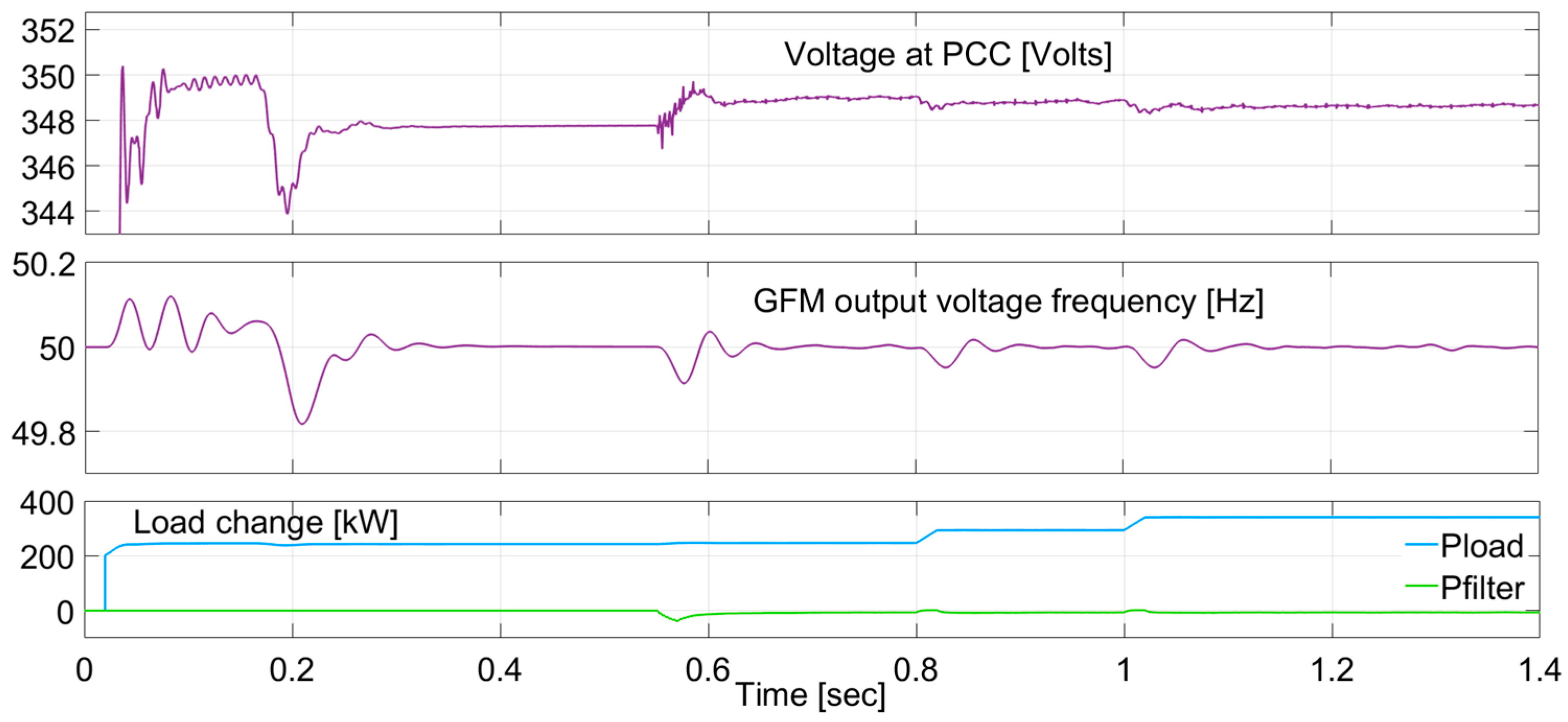
To evaluate how THD responses vary with load step changes, simulations were conducted under sequential disturbances including load increments, SAF activation, and fault events (from 240 kW to 340 kW). In the first scenario, the SAF is activated at 0.55 s, followed by load increases at 0.8 s and 1.0 s. A sensitivity analysis has been performed to observe THD variation under different load levels, as shown in Figure 7 and

Table 2. Current THD and PCC voltage under varying load conditions.

Load (kW)	THD in IGFM (% of Fundamental)	THD in IPCC	PCC Voltage (Volts)	Remark
240	4.52	19.59	347.8	SAF inactivate
242.9	2.12	3.68	348.8	SAF activate
290	2.03	4.21	346.6
340	2.01	5.41	348.5

. The inverter current THD remains consistently low (around 2%) across load steps. The voltage at the PCC and output frequency remain stable with minimal oscillations, indicating that THD remains well controlled under load steps. Despite load increases and a sudden voltage dip during the fault, the system demonstrates strong recovery, with PCC voltage and frequency quickly returning to nominal levels. Additionally, voltage recovery after fault events was evaluated under different load steps, and the system consistently demonstrated successful recovery.

Figure 8 illustrates the power flow across various system elements. Prior to 1.2 s, when the SAF is inactive, its power consumption is negligible. After the SAF is activated, it draws 5.1 kW after the transients, accounting for system losses. Over time, SAF’s power consumption sequentially decreases to almost 2 kW. However, the power consumed by the SAF constitutes a system loss. Figure 9 illustrates the voltage and frequency characteristics of a GFM system. In the upper plot, the voltage at the PCC is initially stable at approximately 348 V. At 1.5 s, a severe three-phase fault is introduced, causing the PCC voltage to drop sharply to nearly zero. The fault persists until 1.65 s, after which the voltage gradually recovers and stabilizes. In the lower plot, the frequency response of both the inverter output and the PCC voltage is depicted. Prior to the fault, both frequencies are steady at approximately 50 Hz. During the fault, the inverter frequency exhibits a noticeable transient increase, indicating a temporary over-frequency condition as the inverter control strategy reacts to the severe voltage disturbance.

Meanwhile, the PCC frequency also deviates but follows the inverter response with a slight delay. After the fault is cleared at 1.65 s, both frequencies gradually return to the nominal 50 Hz as the system stabilizes and resumes normal operation. This behavior reflects the typical dynamics of GFMs in response to grid faults, highlighting the impact on both voltage regulation and frequency stability. Figure 10 presents the SAF’s DC link current and voltage profiles. The figure indicates that the DC link voltage stabilizes at a certain level and remains stable, avoiding any collapse throughout the system’s dynamics. The stable DC link voltage ensures reliable SAF performance and demonstrates the effectiveness of consistent operation.

Figure 11 illustrates the active power and frequency dynamics during transitional events. Upon fault occurrence, the GFM exhibits a pronounced active power deviation corresponding to a frequency dip, followed by oscillatory behavior as the system attempts to stabilize. Similarly, the fault event induces a pronounced surge in reactive power demand, accompanied by a substantial overvoltage condition at the PCC, reflecting the system’s transient response. Upon fault clearance, the voltage reverts to its nominal level, indicating the system’s dynamic recovery and stabilization. These observations underscore the GFM’s adaptive modulation of frequency and voltage to maintain operational stability under disturbance conditions.

An inclusive evaluation of GFM control strategies, including standard GFM control, GFM with VI control, GFM with SAF, and GFM with coordinated SAF and VI control, is conducted based on key performance parameters presented in

Table 3. Comparative Evaluation of Grid-Forming Inverter Coordinated Controls.

Parameter	Conventional GFM Control [23,27,28]	GFM with Virtual Impedance (VI) Control [13]	GFM Control with SAF [29,30]	Proposed Work
Harmonic Suppression	Limited; lacks active mitigation	Limited; weak for high-order harmonics	Good; SAF cancels harmonics	Good; works in weak/distorted grids
THD in IGFM	4.22%	4.16%	1.88%	1.82%
THD in Igrid	19.5%	18.21%	3.68%	3.61%
Tunable Parameters	Droop gains, Voltage and frequency reference setpoints	Virtual resistance and reactance values Droop coefficients Voltage and frequency reference setpoints Damping factor for VI	Active and reactive power droop coefficients Voltage and frequency reference setpoints Filter parameters	Droop coefficients VI parameters Damping coefficients Frequency and voltage reference setpoints. Filter parameters
Current limiting response time	${\mathrm{I}}_{peak}=3842 \mathrm{A}$ $∆\mathrm{I}=3359 \mathrm{A}$; $∆{\mathrm{T}}_r=22.18 \mathrm{m}\mathrm{s}$ $∆{\mathrm{T}}_s=93.15 \mathrm{m}\mathrm{s}$ $I_{fault}=1420 \mathrm{A}$	${\mathrm{I}}_{peak}=3861 \mathrm{A}$ $∆\mathrm{I}=3381 \mathrm{A}$; $∆{\mathrm{T}}_r=22.2 \mathrm{m}\mathrm{s}$ $∆{\mathrm{T}}_s=93.7 \mathrm{m}\mathrm{s}$ $I_{fault}=1420 \mathrm{A}$	${\mathrm{I}}_{peak}=1107 \mathrm{A}$ $∆\mathrm{I}=625 \mathrm{A}$; $∆{\mathrm{T}}_r=16.5 \mathrm{m}\mathrm{s}$ $∆{\mathrm{T}}_s=43.7 \mathrm{m}\mathrm{s}$ $I_{fault}=549 \mathrm{A}$	${\mathrm{I}}_{peak}=1109 \mathrm{A}$ $∆\mathrm{I}=629 \mathrm{A}$; $∆{\mathrm{T}}_r=16.8 \mathrm{m}\mathrm{s}$ $∆{\mathrm{T}}_s=44.15 \mathrm{m}\mathrm{s}$ $I_{fault}=548 \mathrm{A}$

.

From Table 3, it is obtained that in the GFM-only case, the inverter current peaked at 3842 A with a rise time ($∆{\mathrm{T}}_r)$ of 22.18 ms, settling at 1420 A after 93.15 ms. The addition of SAF produced a nearly identical response, indicating minimal impact on fault current limitation. However, introducing VIC significantly reduced the peak current to 1107 A, with faster rise (16.5 ms) and settling times ($∆{\mathrm{T}}_s=$ 43.7 ms), and a lower steady-state fault current of 549 A. Similar performance was observed in the combined SAF and VIC case. These results confirm that VIC is the key contributor to effective fault current limitation, while SAF maintains harmonic filtering without compromising this function.

5. Conclusions

The proposed integrated control system for GFMs, incorporating active harmonic mitigation via a SAF and dynamic overcurrent limitation through VIC, demonstrates improved performance under nonlinear and dynamic grid conditions. Analysis reveals that the system effectively regulates THD and fault current magnitudes, ensuring both power quality and component protection. Simulation results under varying nonlinear loading scenarios indicate a suppression of harmonics from the grid and GFM current, ensuring consistent compliance with IEEE-519 power quality standards at the PCC. The virtual impedance-based overcurrent limiting strategy dynamically shapes the inverter output impedance to constrain fault currents within safe limits, ensuring fast current suppression without affecting SAF performance. Importantly, the current profiles of the shunt active filter remain virtually unaffected during fault transients, indicating minimal cross-coupling between the harmonic mitigation and overcurrent-limiting control loops. The simulation results collectively validate the reliability, selectivity, and dynamic resilience of the proposed system, highlighting its suitability for next-generation inverter-dominated power networks.