Abstract
In practical array signal processing applications, direction-of-arrival (DOA) estimation often suffers from degraded accuracy under low signal-to-noise ratio (SNR) and limited snapshot conditions. To address these challenges, we propose an off-grid DOA estimation method based on Fast Variational Bayesian Inference (OGFVBI). Within the variational Bayesian framework, we design a fixed-point criterion rooted in root-finding theory to accelerate the convergence of hyperparameter learning. We further introduce a grid fission and adaptive refinement strategy to dynamically adjust the sparse representation, effectively alleviating grid mismatch issues in traditional off-grid approaches. To address frequency dispersion in wideband signals, we develop an improved subspace focusing technique that transforms multi-frequency data into an equivalent narrowband model, enhancing compatibility with subspace DOA estimators. We demonstrate through simulations that OGFVBI achieves high estimation accuracy and resolution while significantly reducing computational time. Specifically, our method achieves more than 37.6% reduction in RMSE and at least 28.5% runtime improvement compared to other methods under low SNR and limited snapshot scenarios, indicating strong potential for real-time and resource-constrained applications.
1. Introduction
Direction-of-arrival (DOA) estimation, as a crucial branch of array signal processing, has been extensively studied [] and plays a pivotal role in various fields such as radar, sonar, mobile communications, and autonomous driving.
1.1. Subspace Methods
Given that modern wireless communication systems, such as 4G and 5G, predominantly use broadband signals to enhance data transmission rates and spectrum efficiency, this paper focuses on DOA estimation methods based on 5G OFDM signals. In this context, a broadband signal refers to one whose bandwidth is not negligible compared to its carrier frequency, typically characterized by a fractional bandwidth (i.e., the ratio of signal bandwidth to center frequency) exceeding 5–10%, whereas signals with fractional bandwidth below 3–5% are generally treated as narrowband in array processing literature []. This distinction is essential because traditional narrowband DOA models rely on the assumption that all signal frequency components experience nearly identical phase shifts across the array—a condition no longer valid in broadband scenarios []. Existing broadband DOA estimation methods primarily fall into two categories: Maximum Likelihood (ML) [], which suffers from high computational complexity due to multidimensional search, and subspace-based methods, which offer lower complexity by extending narrowband techniques and is more suitable for wideband array signal processing applications.
For broadband DOA estimation, the Coherent Signal Subspace Method (CSSM) [] outperforms incoherent approaches by aligning multi-frequency data via a focusing matrix, enabling narrowband processing while handling coherent sources. Although CSSM reduces computational complexity and maintains robustness under low SNR [,], its performance depends heavily on the initial angle estimation and still faces complexity challenges.
Over the past few decades, narrowband DOA estimation methods have matured significantly, ushering in the era of high-resolution DOA estimation. Subspace-based methods such as MUSIC [,] and ESPRIT [,] achieve high-resolution DOA estimation through signal–noise subspace decomposition. However, they require prior knowledge of source number, high SNR, and sufficient snapshots for accurate covariance estimation, and fail with coherent sources due to multipath effects [,].
1.2. Sparse Bayesian Methods
Recent advances in compressed sensing have transformed array DOA estimation by utilizing signal sparsity in spatial or transformed domains []. This approach reformulates the problem as Sparse Signal Recovery (SSR) [,]. Unlike traditional subspace methods, sparse reconstruction performs better with low SNR and limited snapshots while being more noise-resistant. The key idea is to extract sparse signals from an overcomplete dictionary by identifying key components. While traditional SBL methods work well for these problems, their performance suffers from slow hyperparameter convergence and spatial discretization issues in low-SNR conditions, particularly with parameter circular dependency and grid mismatch.
To solve the parameter circular dependency problem, Luessi et al. [] developed a sparse Bayesian algorithm for multi-measurement vectors. Their method uses iterative maximization within a variational Bayesian framework for accurate hyperparameter estimation. Despite this improvement, block-sparse models still face slow convergence and high computational costs. Subsequent work by Tipping et al. [] accelerated convergence through fast marginal likelihood maximization, while Fang et al. [] improved complex signal handling with mode-coupled learning. However, achieving both fast and accurate reconstruction remains challenging in practice.
While the aforementioned improvements address computational challenges, recent advances in SBL further enhance its capabilities. For example, Refs. [,,,] further focused on reducing computational load by incorporating various real-valued transformations within the compressed sensing framework; Ref. [] introduces a generalized double Pareto (GDP) prior—sparser than the Laplace prior—for improved signal modeling, while [] proposes a spatial alternating method to accelerate convergence. Although these methods show promise, DOA estimation accuracy remains limited under single-snapshot or coarse-grid conditions. Building on these developments, variational sparse Bayesian inference methods [,,,] further refine the SBL framework for enhanced estimation performance.
1.3. On-Grid vs. Off-Grid Challenges
The off-grid problem arises because, within the SSR framework, it is assumed that the true signal DOA lies on some predefined fixed grid points. However, since signal sources are continuously distributed in space, the true DOA always falls outside the grid points, regardless of how fine the grid is. Therefore, when the DOA does not exactly align with the predefined sampling grid points, the performance of these methods degrades due to the off-grid problem. The off-grid problem also occurs in DOA estimation problems involving arrays with special structures, including sparse arrays [] and coprime planar arrays [].
To address this issue, Yang et al. [] proposed an off-grid DOA estimation method based on Sparse Bayesian Learning (OGSBI). Although the OGSBI method effectively achieves off-grid DOA estimation, its performance is less than ideal when using coarse grids. Dai et al. [] introduced a root-off-grid sparse Bayesian DOA estimation method (RootSBL), which improves the accuracy of coarse grid DOA estimation while reducing computational complexity. Subsequently, in [], a second-order Taylor approximation was introduced to reduce approximation errors, addressing the issue of low estimation accuracy with first-order Taylor approximations under coarse grids, though the computational complexity remained relatively high. Additionally, there are off-grid SSR methods that do not rely on grid constraints, such as the method based on atomic norm minimization (ANM) [].
1.4. Deep Learning Methods
Additionally, with the development of machine learning technologies, some studies have begun to explore the application of deep learning techniques to DOA estimation. Currently, most deep learning-based DOA estimation methods adopt classification models. For example, in [], the DeepMUSIC framework is proposed, where the DOA region is divided into subregions, and a CNN is trained for each subregion. In [], under low SNR conditions, the real part, imaginary part, and phase of the covariance matrix are used as three-channel inputs. In [], a residual network is used to model array defects robustly. However, these methods typically require large amounts of training data, and their performance may be affected when the data distribution changes.
Table 1 provides a comparative summary of the above existing DOA estimation methods, highlighting their respective advantages and limitations in practical DOA estimation scenarios.

Table 1.
Comparison of advantages and disadvantages of DOA estimation methods.
1.5. Practical Applications and Implementations of DOA Estimation
DOA estimation is widely used in practical systems, especially in adaptive beamforming. It helps improve spatial resolution and reduce interference. A typical example is the Capon beamformer, also known as the Minimum Variance Distortionless Response (MVDR) algorithm. It minimizes the output power while keeping a distortionless response in the desired direction []. Compared to traditional beamforming, it provides better angular resolution. However, its performance may drop when snapshots are limited or model mismatch occurs.
Furthermore, DOA estimation techniques have been extended to real-time beamsteering hardware. For instance, adaptive DDS-PLL (Direct Digital Synthesizer–Phase-Locked Loop) architectures have been proposed for real-time AoA estimation and dynamic beam control in phased arrays []. Reliable and fast DOA estimation is essential in these systems, highlighting the importance of robust DOA algorithms in practical deployments.
In addition to software-based methods, DOA estimation has also been implemented in hardware. Phase interferometry-based techniques are often used because of their low complexity. These methods allow DOA estimation to run in real time with high efficiency. Reconfigurable digital architectures have also been developed. These can execute DOA algorithms directly in hardware, which is suitable for embedded platforms with strict latency and power limits [].
This paper proposes an off-grid DOA estimation method based on Fast Variational Bayesian Inference (OGFVBI) to address the problems of grid mismatch, slow convergence, and high complexity in existing sparse Bayesian approaches. To the best of our knowledge, this work is the first to combine fixed-point acceleration and dynamic dual-stage grid evolution within a unified variational Bayesian framework. This integration leads to improved estimation accuracy and efficiency, particularly under low SNR and limited snapshot conditions.
The main contributions of this work are threefold:
(1) A fixed-point update scheme is designed within the variational Bayesian inference framework, avoiding slow EM-type updates and improving convergence stability. This addresses the main limitation of real-valued variational Bayesian inference (realVBI) in convergence speed.
(2) A dual-stage grid fission mechanism is developed to dynamically expand and refine the grid using posterior information. This two-phase strategy improves resolution and robustness compared to the single-stage grid refinement in RootSBL.
(3) A frequency-aligned subspace focusing technique is proposed for broadband OFDM signals, enabling covariance reconstruction and compatibility with narrowband DOA methods across subcarriers.
Together, these components form a unified framework that achieves higher accuracy, lower complexity, and faster convergence than previous off-grid Bayesian DOA methods. Simulation results show that the proposed method achieves high estimation accuracy and resolution, while maintaining low computational overhead, especially under low SNR and limited snapshot conditions.
2. Signal Model
Assume there are distant signal sources arriving at an array formed by elements, with the array arranged on a uniform linear array . The element spacing is , where represents the wavelength and the signal’s snapshot number is . The angle of arrival of the signals is .
Considering the first array element as the reference, the array steering vector corresponding to this angle is
The signal received by the m-th array element can be expressed as
where , is the signal from the k-th source arriving at the uniform linear array, is Gaussian white noise, and is the angle of arrival of the k-th source. represents the transpose of the array.
The array data received in this configuration can be expressed in matrix form as
The formula represents the received signal of the array, with ; represents the incoming signal; is Gaussian white noise with a mean of zero, having a high power spectral density, and is independent of the incoming signal; and represents the array steering vector, where the direction of the array is represented by (1).
The received signal from the array can be written in matrix form, as
When the signal sources and noise are uncorrelated, the covariance matrix of the data received by the array elements can be expressed as
where represents the expectation operator; is the signal’s autocorrelation matrix; is the noise power; and is the identity matrix. By performing normalization on (5), we obtain
where represents the vectorization operation; is a dimensional matrix; represents the conjugate transpose operation; and denotes the Khatri–Rao product operation; and is the energy vector of the signal sources.
Due to the assumption that the received signal fills the entire spatial domain with uniform distribution, the entire spatial domain is discretized into grid points, where is the n-th grid point, and . Each grid point represents a potential angle of arrival, thus forming a complete dictionary set
where represents the Kronecker product.
Equation (6) can thus be transformed into a fully sparse representation model:
Based on the actual situation, the signal source’s position is unlikely to be placed neatly on a predefined discretized grid. Therefore, we consider introducing an off-grid model. Suppose is the uniform distribution between grid points, and represents the actual angle of arrival. It does not belong to the grid set, i.e., . In the case of the two grid points, a small step expansion is performed, and for we have
In the equation, the grid mismatch and is the steering vector of , where the matrix is constructed from and . The off-grid model in (9) adopts a first-order Taylor expansion, which is effective when the angular offset between the actual DOA and the nearest grid point is small. However, for coarse grids, this linear approximation may introduce non-negligible errors. In such cases, higher-order expansions (e.g., second-order Taylor series as discussed in []) can be considered to improve the fidelity of the steering vector approximation. Nevertheless, to maintain computational efficiency, the proposed method retains the first-order model while mitigating grid mismatch via adaptive grid evolution and refinement.
Substituting Equation (9) into Equation (7), the complete dictionary set of the off-grid model can be expressed as
where , , , bold lowercase letters (e.g., ) denote vectors, and bold uppercase letters (e.g., ) denote matrices. The operator denotes a diagonal matrix formed from a vector. The notation represents the array steering vector at angle , while denotes its derivative with respect to .
In summary, the off-grid sparse representation model can be expressed as
According to [], when the signal source is a wideband high-frequency signal, the mismatch of the steering vector of the received signal follows a Gaussian distribution. represents the estimated covariance matrix of the actual scenario. The matrix is the ideal covariance matrix, and the estimation error between the two estimates is defined as , where the mismatch follows a Gaussian distribution.
where represents the asymptotic normal distribution, , and is the ideal covariance matrix. Since cannot be directly obtained, the covariance of will be approximated by . Therefore, the normalized sample covariance matrix can be expressed as
Through sparse Bayesian learning, the main difficulty in directly processing Equation (13) is that is unknown and follows a Gaussian distribution, which is not a standard SBL form. To solve this issue, we treat as an unknown part of the signal, i.e.,
where ; is a vector with all elements zero except the m-th element, which is one.
To facilitate sparse Bayesian analysis, we define and , which can be expressed as Equation (14).
3. Methodology
3.1. Traditional DOA Estimation Algorithms
Subspace-based DOA estimation methods have long been regarded as classical techniques in array signal processing, owing to their ability to achieve high-resolution direction estimation. Among them, the most representative is the Multiple Signal Classification (MUSIC) algorithm.
The MUSIC algorithm is based on the eigenvalue decomposition of the covariance matrix of the array received data. It separates the signal and noise subspaces and utilizes their orthogonality to construct a spatial spectrum function. Specifically, the covariance matrix of the data received by the array elements is shown in Equation (5).
After eigenvalue decomposition, the noise subspace is obtained. The MUSIC spatial spectrum is then constructed as follows:
DOA estimates are then determined by searching for the peaks of the MUSIC spatial spectrum, where the steering vector is most orthogonal to the noise subspace.
Although MUSIC achieves excellent resolution under ideal conditions (e.g., high SNR, sufficient snapshots), it has several limitations. It requires prior knowledge of the number of sources and performs poorly when signal sources are coherent or when the number of snapshots is limited. Moreover, it is sensitive to estimation errors in the sample covariance matrix.
In this work, MUSIC serves as a benchmark method for evaluating the performance of the proposed algorithm.
In contrast, SBL-based DOA estimation algorithms can fully utilize the discontinuous virtual element information discarded by subspace-based methods. Even when the number of signal sources to be estimated is unknown, they can still achieve high-precision DOA estimation with limited snapshots.
3.2. Broadband Signal Processing: Focusing Algorithm
Since the goal of this paper is to implement DOA estimation for broadband OFDM signals, it is necessary to first apply a frequency focusing method to preprocess the broadband signal. We adopt an improved subspace-based focusing technique to align the frequency components across subcarriers and reconstruct an equivalent narrowband covariance matrix. This enables the application of the proposed OGFVBI algorithm to estimate DOAs from broadband observations. Compared with the typical Two-sided Correlation Transformation (TCT) method [], the proposed focusing scheme is simpler in construction, thereby lowering computational complexity while maintaining spatial fidelity.
Focusing inevitably alters the signal structure and noise behavior. To ensure that the SNR remains consistent, we apply a normalization criterion such that the focusing matrix is unitary []. Under this condition, the output noise remains Gaussian, and the post-focusing SNR is preserved.
To enable the aforementioned focusing and subspace processing, we make several standard assumptions. First, the signal sources are mutually uncorrelated and located in the far field, leading to planar wavefronts. The received signal comprises multiple subcarrier components, each modeled as narrowband due to the sufficiently small subcarrier spacing. The additive noise at each antenna element is modeled as zero-mean, circularly symmetric complex Gaussian noise, which is temporally and spatially white with identical variance . The received signal can then be rewritten as
where is the array steering matrix, and is the received signal data on subcarrier . The covariance matrix of the received signal can be written as follows:
where is the covariance matrix of , and denotes the covariance matrix of spatially white complex Gaussian noise. The signal subspace of can be obtained through eigenvalue decomposition:
where is the signal subspace, and is the noise subspace. The focusing matrix is constructed as
where is the signal subspace of or , and the calculation formula for is as follows:
The estimate of , denoted as , is as follows:
where and are abbreviations for and , respectively. The optimization problem for can be expressed as
where is the array steering vector, is the covariance matrix of the received signal, is the beamforming weight vector, and are constants.
This optimization problem can be solved using the Lagrange multiplier method:
where is determined by the following equation:
where is the number of array elements and and are the smallest and second smallest eigenvalues of the array’s received signal covariance matrix, respectively. Therefore, we calculate for each angle :
where is determined by the following equation:
where is the eigenvector corresponding to the smallest eigenvalue of .
Thus, the spatial power spectrum is defined as
For each angle this power spectrum is computed and the angle corresponding to its peak is obtained, i.e., the angle and its number obtained by pre-estimation is used as an input to the subsequent algorithm.
Then, using the above calculations, is applied to focus the correlation matrix of the received data as
Since the signal subspace and noise subspace are orthogonal, the focused correlation matrix for all subcarriers can be simplified as
where is the array covariance matrix after focusing, which can replace in Equation (13) in Section 2, and then proceed with the subsequent VBI processing.
When the number of sources is and the number of array elements is , the computational complexity of constructing the focusing matrix in the proposed method is , whereas that of the traditional TCT algorithm is . Since in most practical scenarios, the proposed method offers lower computational complexity and a simpler construction procedure.
In terms of estimation accuracy, the proposed method yields the same eigenvectors of the covariance matrix as the TCT algorithm after focusing. Therefore, it achieves comparable DOA estimation accuracy to that of the TCT method.
3.3. Variational Bayesian Inference
In this work, we adopt variational Bayesian inference (VBI) to estimate the DOA parameters. Compared to EM, which provides only point estimates and can suffer from slow or unstable convergence, VBI estimates full posteriors and improves robustness. While MCMC methods can be accurate, they are computationally intensive and unsuitable for real-time processing.
VBI offers a good balance between accuracy and efficiency by turning inference into an optimization problem with closed-form updates. In our framework, VBI is further accelerated using a fixed-point update scheme and combined with adaptive grid evolution, making it well-suited for fast and scalable off-grid DOA estimation.
Following the variational Bayesian framework, we begin by approximating the posterior distribution of the signal component. Based on the joint likelihood in Equation (15), the update expression for the signal posterior can be derived as follows:
Construct a two-stage hierarchical prior probability density function. Assuming follows a Gaussian distribution, the Gaussian prior probability density function of is
In the equation, , , and the hyperparameter is further assumed to follow an independent Gamma distribution, i.e.,
In the equation, the shape parameter is fixed at 1 to ensure a stronger shrinkage effect on the parameters, causing most of the estimated values to approach zero, thereby achieving sparsity. is a small positive constraint, typically set to 0.01. The Gamma distribution is defined as .
Based on the assumptions of the above Bayesian hierarchical model, the joint distribution of the signal can be obtained:
According to Bayesian theory, the maximum posterior probability of the parameters to be estimated can be obtained, but its calculation usually involves high-dimensional, complex integrals, which are difficult to solve. Therefore, we introduce variational inference to solve the problem of maximum posterior estimation.
In variational inference, the observed data are the array element received data , and the set of latent variables consists of the parameters to be estimated.
In the equation, is the evidence lower bound (ELBO); is the KL divergence, which represents the degree of approximation between the probability distribution and the posterior distribution . The smaller the KL divergence, the higher the approximation. Variational inference aims to maximize the lower bound of by finding the distribution of such that the lower bound of the ELBO is maximized. At this point, can be used to approximate the posterior probability distribution of the latent variables.
To maximize the lower bound, the probability distribution is decomposed as , and the general expression for the optimal approximate distribution is given.
In the equation, is the conditional expectation of the parameter’s approximate distribution for , conditioned on .
3.3.1. Ignore the Terms Unrelated to the Signal
From Equation (36), the best approximate distribution of can be obtained.
The approximate posterior of follows a complex Gaussian distribution, expressed as
where
3.3.2. Ignore the Terms Unrelated to Precision
From Equation (36), the best approximate distribution of can be obtained.
Its approximate distribution is , and the signal precision follows a multidimensional Gamma distribution. The superscript represents the iteration number, and the iterative update expression for its precision is
In the equation, represents the i-th element of the mean vector , and represents the i-th diagonal element of the covariance matrix. Therefore, based on Equations (42) and (43), the update function for can be obtained, i.e., , and its specific form is as follows:
By iteratively updating Equations (39), (40), and (44) until convergence, the solutions for the relevant parameters can be obtained. However, due to the circular dependency of the hyperparameter on and , this may lead to slower convergence of , thus affecting the overall speed of the algorithm.
3.4. Fast Variational Bayesian Inference
To address the issue of parameter circular dependency in the iterative update, this paper incorporates the concept of Fast Variational Bayesian Inference (FVBI) during the parameter iteration phase to effectively accelerate the iterative process.
According to Equation (44), by repeatedly updating the hyperparameter , an estimate sequence can be obtained. If this update sequence converges, the limit must be a fixed point of this recursive relation:
Thus, the convergent solution of the hyperparameter can be obtained by solving the equation . According to reference [], if the initial condition is and the first-order recursive relation is strictly increasing, then when , the limit of is as follows:
where represents the fixed point greater than , represents the fixed point less than or equal to , and represents the empty set.
Since is a strictly decreasing monotonic function with respect to , the update function for the hyperparameter is strictly increasing, so the above conclusion can be applied.
In essence, the proposed Fast Variational Bayesian Inference reformulates the conventional slow, recursive variational EM update into a root-finding problem of a strictly increasing function, as illustrated in Figure 1, thereby enabling faster fixed-point iteration and improving computational efficiency under mild initialization conditions.
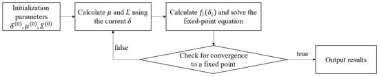
Figure 1.
Fast Variational Bayesian Inference process diagram.
3.5. Grid Evolution
To reduce computational load, the initial grid is kept coarse. However, overly coarse grids may lead to multiple DOAs falling within the same interval, causing traditional methods to fail. This paper proposes a novel grid update method with two components: a fission process to ensure one DOA per grid interval, and an update process to approximate the true DOA. Alternating iterations of these processes refine the grid and improve estimation accuracy. Figure 2 shows a schematic diagram of the grid evolution process.
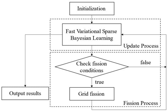
Figure 2.
Grid evolution process diagram.
3.5.1. Update Process
The update of grid refinement is completed during the maximization phase of the Expectation Maximization (EM) algorithm, i.e., .
where
In the equation, ; ; ; denotes the 2-norm of the matrix; denotes the trace of the matrix; represents the Hadamard product; const is a constant; is the vector composed of the first N elements of ; is the last element of ; is the matrix composed of the first N rows and columns of ; and is the vector composed of the first N columns of the N + 1-th row of .
Differentiating Equation (44) and setting it to zero yields the update expression for :
However, this equation requires that is invertible. In practical scenarios, especially under low SNR or when the dictionary is highly coherent, the matrix may become ill-conditioned or even singular. To ensure numerical stability, we adopt a regularized inversion strategy by adding a small damping term:
where is a small positive constant (e.g., ) that ensures invertibility without significantly altering the solution. Alternatively, if the diagonal of is dominant, the simplified component-wise update
can be used as a computationally efficient approximation.
The original off-grid method updates the measurement matrix using the obtained and proceeds to the next iteration. While the updated matrix offers a better approximation of the true steering matrix, the distance between the actual and the nearest grid point remains unchanged. Thus, the modeling error from the off-grid gap in Equation (9) persists. To resolve this, we can treat the grid point positions as adjustable parameters and directly update them.
The overcomplete dictionary set is updated with the refined grid points. After several iterations, the updated grid points will converge towards the true DOA. In practice, candidates are selected based on the refined grid positions. If , the new is accepted; otherwise, the original grid point is kept. The process continues until the stopping condition or is met, where is the error threshold, is the iteration count, and is the maximum number of iterations.
3.5.2. Fission Process
- Fission Strategy
If the energy of the i-th row of is small, indicating the source is not at that position, the corresponding remains unchanged. Therefore, not all grid points need to be updated in each iteration. The maximum number of targets resolvable by an array with elements is . Thus, the grid points corresponding to the top largest energy values of are selected for updating. The average power of is as follows:
The larger the , the higher the likelihood of a DOA in that direction. Thus, only grid intervals with large values require fission. We select the top largest values as candidate grid points for fission. However, when a signal source has large energy, its side lobe energy may surpass the main lobe energy of other sources, potentially leading to the loss of grid points for smaller main lobes. Therefore, the accurate method is to choose the angle positions corresponding to local maxima in the top largest average power values as fission grid points.
Fission generates two new grid points. When the i-th grid point is selected for fission, the new grid points are placed at the midpoints between the and grid intervals. This process continues, progressively approaching the true DOA position.
- 2.
- Iterative Update
When a grid point undergoes fission, new grid points are generated. According to the off-grid model (15), rows corresponding to , and the array manifold matrix for this grid point should be added for the next iteration. The grid interval, RRR, also needs to be recalculated as .
- 3.
- Fission Termination Condition
As the fission process progresses, the number of grid points increases, raising computational complexity. Excessive fission depth can degrade estimation accuracy. Fission stops when the left and right intervals of a grid point III fall below a threshold, i.e., and . The fission termination condition impacts DOA performance.
4. Simulation Results
This section evaluates the performance of the proposed OGFVBI method under wideband signal scenarios and compares it with methods such as MUSIC [], RootSBL [], and realVBI []. The Cramér-Rao Bound (CRB) is adopted as the theoretical benchmark for estimation accuracy variance [].
The signal model is based on wideband signal simulation, considering multiple signal sources. The signals are modulated using 16-QAM and transmitted over an OFDM signal, with the following parameters: OFDM subcarrier size is 1024, and the number of symbols is 16. The experimental setup employs a uniform linear array (ULA) with M = 20 elements and an inter-element spacing of half a wavelength, covering an angular range from −90° to 90°. The initial grid interval is set to 1°. The number of Monte Carlo simulation trials was set to . In all relevant plots, shaded regions around the curves represent ±1 standard deviation calculated over Monte Carlo trials, reflecting the robustness and statistical stability of each algorithm. All simulations were conducted in MATLAB R2022a on a computer equipped with an Intel i7-10710U CPU and 16 GB of RAM.
The CRB is calculated for uncorrelated narrowband sources under a known SNR. Let denote the array manifold matrix and its partial derivative with respect to DOA angles. The Fisher Information Matrix (FIM) is computed as follows:
where is the noise power and is the number of snapshots. The CRB for each DOA parameter is obtained from the diagonal entries of the inverse FIM and converted to degrees:
4.1. Focusing Algorithm Estimation Performance Analysis
To further validate the effectiveness of the proposed focusing method, we compare it against the classical TCT-based focusing technique in terms of resulting spatial spectrum sharpness. Figure 3 shows the spatial power spectrum obtained using both methods under the same signal scenario.
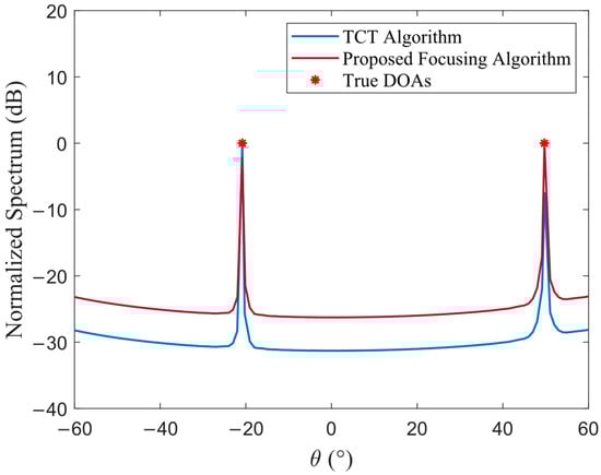
Figure 3.
Spatial power spectrum: proposed focusing algorithm vs. TCT algorithm ().
The spatial spectra of the proposed algorithm and TCT show close agreement, indicating comparable performance. This equivalence occurs because both methods produce identical eigenvectors in the focused covariance matrix. However, the proposed approach achieves this with lower computational complexity.
4.2. Spatial Spectrum Analysis
In the experiments, the DOA of a single source is set to 20.83°, and the corresponding normalized spatial spectrum is shown in Figure 4. For the multiple-source scenario, the DOAs are set to −37.52°, 20.83°, and 49.69°, and the resulting normalized spatial spectrum is shown in Figure 5.
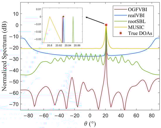
Figure 4.
Normalized spatial spectrum of a single signal source ().
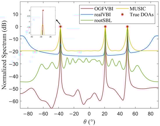
Figure 5.
Normalized spatial spectrum of multiple signal sources ().
Figure 4 and Figure 5, respectively, illustrate the normalized spatial spectrum comparisons of different DOA estimation algorithms under single-source and multi-source scenarios, clearly reflecting the performance differences in terms of localization accuracy and resolution capability. Although all four methods produce spectral peaks that approximately align with the true source locations, the zoomed-in views reveal that the proposed method consistently achieves precise alignment with the true DOAs in both scenarios. The spectral peaks are sharp, with concentrated main lobes and strong sidelobe suppression, and the overall spectrum is smooth and stable—demonstrating superior estimation accuracy and spatial resolution.
In the single-source case shown in Figure 4, the proposed method remains precisely aligned with the true DOA even in the zoomed-in view, indicating its high sensitivity to small angular variations. In contrast, the MUSIC and RootSBL methods exhibit noticeable deviations. Although the realVBI method aligns with the main peak, it suffers from significant sidelobe fluctuations and contains several false peaks, which may lead to misjudgments.
Figure 5 further validates the robustness of the proposed method in multi-source environments. It clearly resolves all three sources, while other algorithms, such as MUSIC and realVBI, exhibit insufficient resolution due to high sidelobes or shifted main peaks.
These results demonstrate that the proposed method maintains high accuracy and resolution even under challenging conditions such as limited snapshots, low SNR, and coarse grids. This advantage stems from the adoption of Fast Variational Bayesian inference combined with a grid adaptation mechanism, which effectively overcomes the performance bottlenecks of traditional methods caused by grid mismatch or slow hyperparameter convergence.
4.3. Resolution Analysis
To determine whether the estimation method can successfully resolve two closely spaced signal sources, the following two conditions must be satisfied:
in the equation, and represent the estimated values corresponding to the true angles and , respectively. is the set angle error threshold, which is set to 0.5° here. denotes the number of successful resolutions in Monte Carlo trials where both incident sources are correctly resolved within the angular error threshold.
Consider two closely spaced, uncorrelated signals arriving at the array from directions and , respectively, with fixed at 20.8°. The angular separation is varied from 1° to 10° in 1° increments. The resulting resolution success rate as a function of angular separation is plotted in Figure 6.
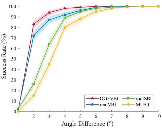
Figure 6.
Resolution success rate (%) as a function of angular separation (◦) ().
Figure 6 illustrates the trend of resolution success rate versus angular separation for four different algorithms under varying angle differences between two signal sources. For different incident signal grid spacings, the method proposed in this paper achieves a resolution success rate close to 100% when the angle interval is 4°. In contrast, the realVBI and RootSBL methods require a grid spacing of more than 6° to achieve a 100% resolution success rate. The MUSIC method, under the same conditions, requires the incident signal grid spacing to be increased to 8° to successfully resolve. It can be observed that the method proposed in this paper consistently maintains a significant performance advantage across the entire angle interval range, particularly in small angle intervals, where its resolution success rate is far higher than that of realVBI, RootSBL, and MUSIC, making it particularly suitable for complex real-world environments with low SNR and small angle differences between sources. The reason for this is that the method introduces a dynamic grid fission and update mechanism, allowing the algorithm to progressively refine the grid and approach the true signal source position even when starting with a coarse grid, significantly improving resolution. In contrast, traditional methods such as MUSIC heavily rely on the orthogonality of signal subspaces and a high number of snapshots, making them extremely sensitive to small angle differences and highly correlated signals, which can lead to subspace leakage and resolution failure. Although RootSBL and realVBI somewhat address the grid discretization issue, they still depend on fixed grids, which may cause aliasing or spectral peak merging when dealing with closely spaced sources.
Consider two closely spaced, uncorrelated signals impinging on the array from directions 20.8° and 24.8°, respectively. The resulting resolution success rate as a function of SNR is shown in Figure 7.
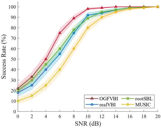
Figure 7.
Resolution success rate (%) versus SNR (dB) ().
Figure 7 shows the resolution success rate variation of four DOA estimation algorithms under different SNR conditions. It is clearly observed that as the SNR increases, the resolution capability of all algorithms improves. However, the method proposed in this paper consistently outperforms the others across the entire SNR range, especially showing significantly higher resolution success rates in the low SNR segment.
It can be seen that even under low SNR conditions, where the signal is severely overwhelmed by noise, the proposed method can still reliably extract sparse signal features and gradually approach the true DOA position. In contrast, although the realVBI and RootSBL methods are also based on Bayesian modeling, they have a stronger dependence on hyperparameters and do not address the grid adaptation issue. As a result, they are prone to getting trapped in erroneous local estimates and fail to resolve correctly at low SNR. As the SNR increases further, the resolution of all methods gradually improves. However, the proposed method still maintains close to 100% success rate in high SNR conditions, demonstrating its excellent robustness and resolution ability across the entire SNR range. This shows that the method performs exceptionally well in environments with strong interference and is well-suited for complex scenarios with low SNR and closely spaced signal sources.
4.4. Estimation Accuracy Analysis
The estimation errors of different methods are evaluated using the Root Mean Square Error (RMSE). The RMSE of the estimated directions of incident signals is defined as follows:
where denotes the estimated direction of the k-th signal in the -th Monte Carlo simulation.
In the experiment, three signal sources are set at directions of −37.5°, 20.8°, and 49.6°. The RMSEs of different methods are calculated under varying SNR conditions, and the results are shown in Figure 8. It can be seen that the proposed method consistently maintains the lowest estimation error across the entire SNR range and gradually approaches the CRB curve as the SNR increases.
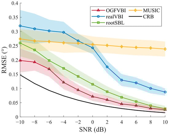
Figure 8.
RMSE (◦) vs. SNR (dB) comparisons of the various methods ().
For example, at an SNR of 0 dB, the RMSE of the proposed method is 0.0717, which improves by 70.5% compared to the 0.2428 of the realVBI method, 37.6% compared to the 0.1147 of the RootSBL method, and 71.8% compared to the 0.2544 of the MUSIC method. The standard deviation of the proposed method is also lower across all SNR levels, indicating more consistent estimation results. These results show that the proposed method quickly converges to the true DOA under low SNR and effectively avoids hyperparameter dependency, demonstrating strong robustness and high accuracy. In contrast, realVBI converges more slowly and often gets trapped in local minima, RootSBL suffers from bias in noisy conditions, and MUSIC is highly sensitive to covariance estimation errors, causing sharp performance drops at low SNR.
With all other experimental parameters held constant, Figure 9 shows the RMSE of different methods under varying snapshot numbers. The estimation errors of all methods decrease as the number of snapshots increases. However, the proposed method consistently achieves the lowest RMSE with smaller standard deviation, indicating more stable and reliable estimates. When snapshots reach 1000, the proposed method’s RMSE is 0.0341, improving by 85.5% compared to MUSIC (0.2353), 70.1% compared to realVBI (0.1140), and 29.4% compared to RootSBL (0.0483). These results demonstrate that the proposed method efficiently uses limited snapshots for accurate DOA estimation, showing strong robustness and practical value.
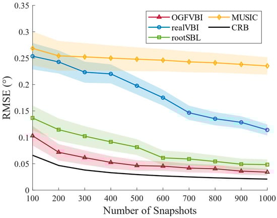
Figure 9.
RMSE (◦) vs. number of snapshots comparisons of the various methods ().
4.5. Efficiency Analysis: Runtime and Convergence
Considering the impact of SNR on computational efficiency, we keep other conditions unchanged and vary the SNR from −10 to 10 in steps of 2. The runtime of different methods under varying SNRs is recorded, as shown in Figure 10. It can be seen that the runtimes of OGFVBI, realVBI, and MUSIC remain relatively stable across different SNR levels, demonstrating good consistency. In contrast, the runtime of the RootSBL method is significantly higher than the others and slightly decreases as the SNR increases, showing larger overall fluctuations.
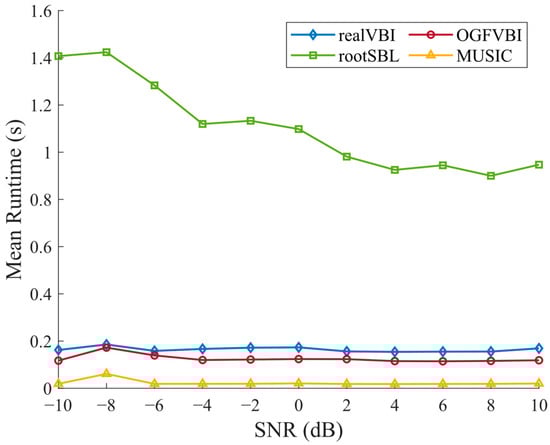
Figure 10.
Mean runtime(s) vs. SNR (dB) comparisons of the various methods ().
Further analysis of the average iteration counts, runtimes, and their corresponding standard deviations for the methods is presented in Table 2.
Table 2.
Computational efficiency and convergence metrics of compared methods ().
Compared to RootSBL and realVBI, our proposed OGFVBI reduces the average runtime by approximately 88.7% and 28.5%, respectively. It also converges with about 65.4% fewer iterations than RootSBL and 48.6% fewer iterations than realVBI. These results confirm the significant computational efficiency gained through the fast variational update and adaptive grid fission strategy used in OGFVBI. Moreover, the relatively low standard deviation in runtime indicates that OGFVBI maintains stable performance across different trials.
4.6. Ablation Study
To evaluate the contributions of the key modules in the proposed OGFVBI algorithm, we performed ablation experiments by separately removing the Fast VBI module and the grid fission module. The results on RMSE, standard deviation, runtime, and runtime variability are jointly analyzed to illustrate their impact.
As shown in Figure 11 and Table 3, the complete OGFVBI model achieves the lowest RMSE values across all SNR levels, with results closely approaching the theoretical CRB bound, demonstrating high estimation accuracy and stability (low standard deviation). Correspondingly, it also attains the shortest average runtime of 0.1238 s with a standard deviation of 0.1255 s, indicating efficient and stable computations.
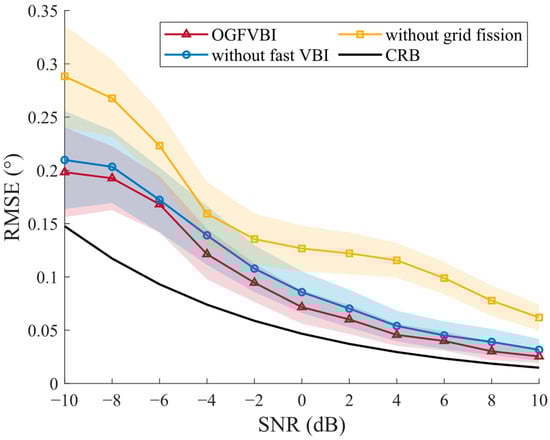
Figure 11.
Ablation study of OGFVBI: impact of grid fission and Fast VBI on estimation accuracy ().
Table 3.
Computational performance comparison of OGFVBI and ablated versions ().
When the Fast VBI module is removed, the RMSE increases slightly across all SNRs, and the standard deviation also rises, indicating degraded accuracy and less stable convergence. Meanwhile, the average runtime significantly increases to 0.1716 s (about 39% longer), with higher runtime variability (standard deviation 0.1828 s). This confirms that the fixed-point acceleration scheme in Fast VBI effectively reduces iteration counts, stabilizes the hyperparameter update process, and thus improves both convergence speed and computational efficiency.
Removing the grid fission module causes a more pronounced increase in RMSE, especially at low SNR values, and larger variability in estimation error. Although the runtime increase is moderate (to 0.1378 s) with a slight rise in standard deviation (0.1468 s), the loss of adaptive grid refinement leads to higher grid mismatch errors, reducing the estimation resolution and accuracy.
In summary, the Fast VBI module primarily enhances convergence speed and runtime stability, while the grid fission module plays a crucial role in reducing grid mismatch and improving estimation precision. Both modules jointly enable OGFVBI to achieve its superior performance in wideband DOA estimation tasks.
4.7. Limitations and Future Extensions
Despite the advantages of the proposed OGFVBI method in terms of accuracy, robustness, and computational efficiency, several limitations and open challenges remain to be addressed in future work.
First, the performance of the algorithm is influenced by the initial grid resolution used to discretize the angular domain. Although the proposed dual-stage grid fission strategy can adaptively refine the grid and alleviate the mismatch between true angles and grid points, the method may still exhibit sensitivity to poor initial settings, especially when the angular search space is large or densely populated with sources. Future improvements could focus on fully gridless approaches or grid initialization strategies guided by prior knowledge.
Second, the algorithm assumes that the number of sources is known and that the sources are mutually uncorrelated. In practical applications, however, these assumptions may not hold. The presence of coherent or closely spaced sources may degrade the performance of subspace-based focusing and reduce the effectiveness of the sparse Bayesian recovery. Similarly, when the number of active sources is over- or under-estimated, the variational updates may either converge slowly or produce biased solutions. An adaptive model selection mechanism or automatic relevance determination could help address such model mismatch issues.
Third, the method is derived under the assumption of white Gaussian noise. In real-world systems, noise may exhibit impulsive, colored, or non-Gaussian behavior due to hardware imperfections, environmental interference, or calibration errors. Under such conditions, the covariance estimation and the posterior inference steps may become biased. Incorporating robust noise modeling or outlier mitigation strategies is a potential direction to improve the applicability of the method.
Beyond these current limitations, the method also has room for extension and generalization. In its present form, the proposed algorithm supports one-dimensional DOA estimation using ULA. In many practical scenarios, however, two-dimensional or even three-dimensional DOA estimation is required—such as in MIMO radar, acoustic sensing, or mmWave vehicular systems. Extending OGFVBI to handle joint azimuth and elevation estimation using uniform rectangular arrays (URA) or uniform circular arrays (UCA) would significantly enhance its spatial resolution and application scope.
Additionally, the method currently assumes far-field signal propagation where planar wavefronts are valid. In near-field scenarios—such as indoor localization or short-range radar—the signal wavefronts are spherical, and the array manifold becomes range-dependent. Adapting the OGFVBI framework to near-field models would allow simultaneous estimation of both direction and distance, enabling integrated localization and tracking applications with a single station.
Finally, from a system implementation perspective, the low complexity and fast convergence properties of OGFVBI make it attractive for real-time embedded applications. Potential deployment scenarios include joint communication and sensing (ISAC) systems, autonomous navigation platforms, and mobile edge computing for intelligent vehicles. Future work will explore how to integrate the algorithm with hardware constraints, dynamic tracking, and low-latency signal processing requirements.
5. Conclusions
This paper addresses the issues of low estimation accuracy, slow convergence, and high computational complexity in existing DOA estimation algorithms under conditions of low SNR, few snapshots, and coarse grids. We propose an off-grid DOA estimation method based on Fast Variational Bayesian Inference (OGFVBI). The method is based on the framework of variational Bayesian inference and approximates the posterior distribution by maximizing the evidence lower bound. A fast fixed-point detection mechanism is introduced to efficiently update hyperparameters, significantly accelerating the algorithm’s convergence and reducing its computational complexity. At the same time, grid fission and adaptive updating strategies are combined to evolve the grid to gradually approach the true source direction, effectively alleviating the grid mismatch problem in traditional off-grid models. In addition, an improved frequency focusing method is designed, which approximates broadband signals as narrowband models, further expanding the algorithm’s applicability in broadband conditions. Simulation results show that the proposed method outperforms existing mainstream methods in estimation accuracy, resolution, and computational efficiency, especially in harsh environments with low SNR and fewer snapshots, demonstrating significant advantages and strong practical applicability and potential for broader use.
Author Contributions
Conceptualization, Z.D. and E.H.; methodology, X.T., Z.D. and E.H.; software, Y.C.; validation, X.T. and Y.C.; formal analysis, Y.C.; investigation, X.T.; resources, E.H.; data curation, Y.C. All authors have read and agreed to the published version of the manuscript.
Funding
This research was funded by the National Key Research and Development Program of China (grant number: 2022YFB3904702) and the National Natural Science Foundation of China under Grant: 6220020330.
Data Availability Statement
The data presented in this study are available within the article.
Conflicts of Interest
The authors declare no conflict of interest.
References
- Molaei, A.M.; Zakeri, B.; Andargoli, S.M.H.; Abbasi, M.A.B.; Fusco, V.; Yurduseven, O. A comprehensive review of direction-of-arrival estimation and localization approaches in mixed-field sources scenario. IEEE Access 2024, 2, 65883–65918. [Google Scholar] [CrossRef]
- Stutzman, W.L.; Thiele G, A. Antenna Theory and Design; John Wiley & Sons: Hoboken, NJ, USA, 2012. [Google Scholar]
- Yang, Y.; Lu, R.; Gao, L.; Gong, S. 4.5 GHz lithium niobate MEMS filters with 10% fractional bandwidth for 5G front-ends. J. Microelectromechanical Syst. 2019, 28, 575–577. [Google Scholar] [CrossRef]
- Stoica, P.; Sharman, K.C. Maximum likelihood methods for direction-of-arrival estimation. IEEE Trans. Acoust. Speech Signal Process. 1990, 38, 1132–1143. [Google Scholar] [CrossRef]
- El-Khamy, S.E.; El-Shazly, A.M.; Eltrass, A.S. A new computationally efficient approach for high-resolution DOA estimation of wideband signals using compressive sensing. IEEE 2023, 1, 74–81. [Google Scholar]
- Hung, H.; Kaveh, M. Focussing matrices for coherent signal-subspace processing. IEEE Trans-Actions Acoust. Speech Signal Process. 1988, 36, 1272–1281. [Google Scholar] [CrossRef]
- Valaee, S.; Kabal, P. Wideband array processing using a two-sided correlation transformation. IEEE Trans. Signal Process. 1995, 43, 160–172. [Google Scholar] [CrossRef] [PubMed]
- Schmidt, R. Multiple emitter location and signal parameter estimation. IEEE Trans. Signal Process. 1986, 34, 276–280. [Google Scholar] [CrossRef]
- Wu, C.; Ye, C. DOA estimation for unfolded coprime arrays: Successive-MUSIC algorithm. IOP Conf. Ser. Mater. Sci. Eng. 2020, 719, 012035–012041. [Google Scholar] [CrossRef]
- Zhang, W.; Han, Y.; Jin, M.; Li, X.S. An improved ESPRIT-like algorithm for coherent signals DOA estimation. IEEE Commun. Lett. 2019, 24, 339–343. [Google Scholar] [CrossRef]
- Wang, R.; Wang, Y.; Li, Y.; Cao, W.; Yan, Y. Geometric algebra-based ESPRIT algorithm for DOA estimation. Sensors 2021, 21, 5933. [Google Scholar] [CrossRef]
- Wax, M.; Adler, A. Direction of arrival estimation in the presence of model errors by signal subspace matching. Signal Process. 2021, 181, 107900–107913. [Google Scholar] [CrossRef]
- Gao, W.; Zhu, S.; Li, X.; Wang, H.; Wang, L. Frequency-difference MUSIC: A method for DOA estimation in inhomogeneous media. Signal Image Video Process. 2024, 18, 7029–7040. [Google Scholar] [CrossRef]
- Fang, Y.; Zhu, S.; Gao, Y.; Zeng, C. DOA estimation for coherent signals with improved sparse representation in the presence of unknown spatially correlated Gaussian noise. IEEE Trans. Veh. Technol. 2020, 69, 10059–10069. [Google Scholar] [CrossRef]
- Liu, B.; Matsushita, S.; Xu, L. DOA estimation with small snapshots using weighted mixed norm based on spatial filter. IEEE Trans. Veh. Technol. 2020, 69, 16183–16187. [Google Scholar] [CrossRef]
- Liu, Y.; Dong, N.; Zhang, X.; Zhao, X.; Zhang, Y.; Qiu, T. DOA estimation for massive MIMO systems with unknown mutual coupling based on block sparse Bayesian learning. Sensors 2022, 22, 8634. [Google Scholar] [CrossRef]
- Luessi, M.; Babacan, S.D.; Molina, R.; Katsaggelos, A.K. Bayesian simultaneous sparse approximation with smooth signals. IEEE Trans. Signal Process. 2013, 61, 5716–5729. [Google Scholar] [CrossRef]
- Tipping, M.E.; Faul, A.C. Fast Marginal Likelihood Maximisation for Sparse Bayesian Models. In Proceedings of the Ninth International Workshop on Artificial Intelligence and Statistics, Key West, FL, USA, 3–6 January 2003; pp. 276–283. [Google Scholar]
- Fang, J.; Shen, Y.; Li, H.; Wang, P. Pattern-coupled sparse Bayesian learning for recovery of block-sparse signals. IEEE Trans. Signal Process. 2015, 63, 360–372. [Google Scholar] [CrossRef]
- Dai, J.; So, H.C. Real-valued sparse Bayesian learning for DOA estimation with arbitrary linear arrays. IEEE Trans. Signal Process. 2021, 69, 4977–4990. [Google Scholar] [CrossRef]
- Liu, D.; Zhao, Y. Real-valued sparse Bayesian learning algorithm for off-grid DOA estimation in the beamspace. Digit. Signal Process. 2022, 121, 103322–103328. [Google Scholar] [CrossRef]
- Zeng, H.; Yue, H.; Cao, J.; Zhang, X. Real-valued direct position determination of quasi-stationary signals for nested arrays: Khatri–Rao Subspace and Unitary Transformation. Sensors 2022, 22, 4209. [Google Scholar] [CrossRef]
- Wang, G.; Kang, Y.; Wang, H. Low-Complexity DOA Estimation Algorithm based on Real-Valued Sparse Bayesian Learning. Circuits Syst. Signal Process. 2024, 43, 4319–4338. [Google Scholar] [CrossRef]
- Wang, Q.; Yu, H.; Li, J.; Ji, F.; Chen, F. Sparse Bayesian learning using generalized double Pareto prior for DOA estimation. IEEE Signal Process. Lett. 2021, 28, 1744–1748. [Google Scholar] [CrossRef]
- Guo, Q.; Xin, Z.; Zhou, T.; Xu, S. Off-grid space alternating sparse Bayesian learning. IEEE Trans. Instrum. Meas. 2023, 72, 1–10. [Google Scholar] [CrossRef]
- Zhang, Y.; Yang, Y.; Yang, L. Off-grid DOA estimation through variational Bayesian inference in colored noise environment. Digit. Signal Process. 2021, 111, 102967–102981. [Google Scholar] [CrossRef]
- Wang, P.; Yang, H.; Ye, Z. An off-grid wideband DOA estimation method with the variational Bayes expectation-maximization framework. Signal Process. 2022, 193, 108423–108430. [Google Scholar] [CrossRef]
- Wang, H.; Wang, X.; Huang, M.; Wan, L. A novel variational SBL approach for off-grid DOA detection under nonuniform noise. Digit. Signal Process. 2022, 128, 103622–103630. [Google Scholar] [CrossRef]
- Fu, H.; Dai, F.; Hong, L. Off-grid error calibration for DOA estimation based on sparse Bayesian learning. IEEE Trans. Veh. Technol. 2023, 72, 16293–16307. [Google Scholar] [CrossRef]
- Liu, Y.; Zhang, Z.; Zhou, C.; Yan, C.; Shi, Z. Robust variational Bayesian inference for direction-of-arrival estimation with sparse array. IEEE Trans. Veh. Technol. 2022, 71, 8591–8602. [Google Scholar] [CrossRef]
- Zheng, H.; Zhou, C.; Shi, Z.; Yan, C.; Shi, Z. Coarray tensor direction-of-arrival estimation. IEEE Trans. Signal Process. 2023, 71, 1128–1142. [Google Scholar] [CrossRef]
- Yang, Z.; Xie, L.; Zhang, C. Off-grid direction of arrival estimation using sparse Bayesian inference. IEEE Trans. Signal Process. 2012, 61, 38–43. [Google Scholar] [CrossRef]
- Dai, J.; Bao, X.; Xu, W.; Chang, C. Root sparse Bayesian learning for off-grid DOA estimation. IEEE Signal Process. Lett. 2016, 24, 46–50. [Google Scholar] [CrossRef]
- Huang, H.; So, H.C.; Zoubir, A.M. Off-grid direction-of-arrival estimation using second-order Taylor approximation. Signal Process. 2022, 196, 108513–108519. [Google Scholar] [CrossRef]
- Wagner, M.; Park, Y.; Gerstoft, P. Gridless DOA estimation and root-MUSIC for non-uniform linear arrays. IEEE Trans. Signal Process. 2021, 69, 2144–2157. [Google Scholar] [CrossRef]
- Elbir, A.M. DeepMUSIC: Multiple signal classification via deep learning. IEEE Sens. Lett. 2020, 4, 1–4. [Google Scholar] [CrossRef]
- Papageorgiou, G.K.; Sellathurai, M.; Eldar, Y.C. Deep networks for direction-of-arrival estimation in low SNR. IEEE Trans. Signal Process. 2021, 69, 3714–3729. [Google Scholar] [CrossRef]
- Li, J.; Shao, X.; Li, J.; Ge, L. Direction of arrival estimation of array defects based on deep neural network. Circuits Syst. Signal Process. 2022, 41, 4906–4927. [Google Scholar] [CrossRef]
- Mestre, X.; Lagunas, M.A. Finite sample size effect on minimum variance beamformers: Optimum diagonal loading factor for large arrays. IEEE Trans. Signal Process. 2005, 54, 69–82. [Google Scholar] [CrossRef]
- Florio, A.; Coviello, G.; Talarico, C.; Avitabile, G. Adaptive DDS-PLL Beamsteering Architecture based on Real-Time Angle-of-Arrival Estimation. In Proceedings of the 2024 IEEE 67th International Midwest Symposium on Circuits and Systems (MWSCAS), Springfield, MA, USA, 11–14 August 2024; pp. 628–631. [Google Scholar]
- Florio, A.; Avitabile, G.; Talarico, C.; Coviello, G. A Reconfigurable Full-Digital Architecture for Angle of Arrival Estimation. IEEE Trans. Circuits Syst. I Regul. Pap. 2023, 71, 1443–1455. [Google Scholar] [CrossRef]
- Möderl, J.; Leitinger, E.; Fleury, B.H.; Pernkopf, F.; Witrisal, K. Fast variational block-sparse Bayesian learning. arXiv 2023, arXiv:2306.00442. [Google Scholar]
- Stoica, P.; Nehorai, A. MUSIC, maximum likelihood, and Cramer-Rao bound. IEEE Trans. Acoust. Speech Signal Process. 2002, 37, 720–741. [Google Scholar] [CrossRef]
Disclaimer/Publisher’s Note: The statements, opinions and data contained in all publications are solely those of the individual author(s) and contributor(s) and not of MDPI and/or the editor(s). MDPI and/or the editor(s) disclaim responsibility for any injury to people or property resulting from any ideas, methods, instructions or products referred to in the content. |
© 2025 by the authors. Licensee MDPI, Basel, Switzerland. This article is an open access article distributed under the terms and conditions of the Creative Commons Attribution (CC BY) license (https://creativecommons.org/licenses/by/4.0/).