Abstract
In this article, we propose a novel near-field holographic microwave imaging technique designed to accelerate the data acquisition process. The system employs a novel electronic switching mechanism utilizing two switching networks that virtually rotate the transmitting and receiving antennas along the azimuthal direction for efficient data collection. This minimizes the need for mechanical scanning of the antennas which, in turn, leads to faster data acquisition. To enhance the quality of the imaging outcome, the number of samples can be increased by combining only a few mechanical scanning steps with the electronic scanning. This data acquisition scheme leverages the system’s space-invariant property to enable convolution-based near-field holographic microwave image reconstruction. By capturing and processing scattered fields over a cylindrical aperture, the system achieves high-resolution imaging of concealed objects across multiple range positions. Both simulation and experimental results validate the effectiveness of the proposed approach in delivering high-quality imaging results. Its ability to provide faster and enhanced imaging outcomes highlights its potential for a wide range of applications, including biomedical imaging, security screening, and non-destructive testing of the materials.
1. Introduction
Microwave imaging (MWI) has emerged as a transformative technology in various fields due to its ability to penetrate optically opaque materials. Its applications span across various domains, including non-destructive testing (NDT) of industrial materials [1,2], biomedical imaging for early disease detection [3,4], and security screening for concealed threat identification [5,6].
Holographic MWI techniques offer high-speed qualitative imaging capabilities. Traditional holographic systems often rely on the acquisition of wideband data to obtain range resolution [5,7]. Although they have been successfully employed for applications such as security screening of passengers at airports [5], they depend on approximations that restrict their applicability in near-field scenarios, where finer spatial details are critical. In particular, far-field holographic imaging techniques fail to capture and process the evanescent waves emanated by the objects, limiting their resolution and accuracy. To overcome these challenges, near-field holographic imaging systems have been developed to obtain higher resolutions by processing the measured portion of the evanescent waves [8].
In general, the near-field holographic imaging approach, which leverages measured point spread functions (PSFs), provides several advantages over the conventional farfield holographic imaging techniques, including the following: (1) Measured PSFs accurately capture the near-field behavior of the antennas used in the specific imaging setup, leading to more realistic system modeling. (2) Unlike analytical PSFs in the far-field holography, which assume scalar far-field values at isolated points, measured PSFs represent actual responses such as S-parameters or terminal voltages. (3) Measured PSFs reflect the true electromagnetic properties of the background medium and include the effects of all components in the imaging system—such as antennas, positioners, and measurement chambers—avoiding the oversimplified assumptions used in far-field holography. (4) By using a calibrated scattering probe of known material and size, the system’s sensitivity to contrast can be quantified. This enables accurate and quantitative imaging [9,10]. (5) The system of equations solved in near-field holographic imaging at each spectral point is smaller and better conditioned than those in optimization-based microwave imaging methods [11]. This not only improves the computational efficiency but also allows for natural parallelization, as each spectral point can be processed independently. (6) Near-field holographic imaging eliminates the need for interpolation in the spectral domain (as implemented in far-field holography [8]), simplifying the reconstruction process. (7) Unlike far-field holographic imaging, near-field holographic imaging does not rely on the assumption that the spatial frequency variables are independent, thereby reducing reconstruction artifacts. (8) Data from multiple antennas, including both forward- and back-scattered signals, can be combined within a single linear system to enhance spatial resolution and reduce image artifacts. (9) Near-field holographic imaging performs effectively with a smaller number of frequency samples, particularly when multiple transmitter/receiver channels are used. This contrasts with far-field holography, which requires densely sampled frequencies due to its reliance on a three-dimensional (3D) inverse Fourier transform.
We emphasize that the near-field holographic imaging technique is based on the Born approximation, which assumes that the incident field in the presence of the object is the same as the incident field in the absence of the object. This assumption linearizes the scattering integral and allows for the use of convolution theory (which holds only for linear systems). However, it provides the best results primarily for small or low-contrast objects (weak scatterers).
In particular, the condition for applying the first-order Born approximation is that the radius a of a sphere enclosing the object and its refractive index n need to satisfy (n− 1)a < /4, where is the wavelength in the background medium [12,13]. Thus, when the objects or their contrasts (with respect to the background medium) become larger, or when there are multiple objects inside the imaged domain, the Born assumption imposes imaging errors due to further disturbance of the linearity of the imaging system.
This challenge can be overcome using iterative optimization methods such as the Born iterative method (e.g., see [14]), distorted Born iterative method (e.g., see [15]), hybrid Born–Rytov method (e.g., see [10]), Newton-type methods (e.g., see [16]), contrast source inversion (e.g., see [17]), or hybrid and data-driven techniques such as machine learning/deep learning techniques (e.g., see [18]), etc. However, these techniques have certain drawbacks in practical applications, including being extremely demanding in terms of memory and time, sensitivity to initial guess, ill-posedness of the solution, and the requirement for large datasets.
Although near-field holographic imaging techniques initially required wideband information to perform three-dimensional (3D) imaging [19], later these techniques used a receiver antenna array to perform 3D imaging using narrow-band data [20]. Narrow-band near-field holographic imaging systems have also been developed for cylindrical setups, where an array of receiver antennas collects scattered fields while rotating, together with the transmitter antenna, around the imaged medium [21]. Despite these advancements, significant obstacles to employing these techniques in applications demanding high-speed imaging remain. In particular, in [21], data acquisition time is a burden since responses need to be collected over a cylindrical aperture by mechanically scanning a transmitter and an array of receiver antennas.
To speed up the data acquisition, electronic scanning of an antenna array can be used instead of mechanical scanning. One method is using a two-dimensional (2D) array of antennas covering the aperture (e.g., see [22]). However, this method is costly due to the use of a large number of antennas and the switching network to control the data acquisition. Another common method that alleviates the cost issue involves arranging antenna arrays in one direction while mechanically scanning them along the perpendicular direction (e.g., see [23,24,25]). Thus, in this work, we take this principle into practice and we build a system featuring the space-invariant property by mimicking mechanical scanning along the azimuthal axis as implemented in [21] via an array of antennas switched electronically. The system’s space-invariant property means that when an object shifts along the cross-range direction (azimuthal or longitudinal directions), its response remains the same but shifts with the same amount and along the same direction [26]. This allows the scattered field measurements to be modeled as a convolution between the point spread function (PSF) and the object’s reflectivity profile, enabling efficient image reconstruction using Fourier-based techniques [8]. To build such a system, we develop a novel switching mechanism utilizing two switching networks that virtually (electronically) rotate the transmitter and the array of receivers around the imaged medium for data collection. While mechanical scanning is still required along the longitudinal axis, the electronic data collection along the azimuthal axis expedites the data acquisition process significantly. We also demonstrate the possibility of collecting more samples along the azimuthal axis via combining a few mechanical scanning steps with the electronic scanning. This alleviates the coarse sampling in the electronic scanning scheme, leading to further enhancement of the reconstructed images. The performance of the proposed imaging techniques will be demonstrated via simulation results and experiments.
2. Methodology
This work proposes a microwave imaging system comprising an array of antennas uniformly distributed along the azimuthal axis to cover the full circular aperture. The angular separation between adjacent antennas is denoted by . In this configuration, microwave switches are used to control the antenna operations such that, at each electronic scanning step, one antenna functions as the transmitter while a set of antennas positioned on the opposite side of the imaging domain act as receivers. Also, we present an approach to increase the number of samples along the azimuthal direction by adding a few mechanical scanning steps in the azimuthal direction.
2.1. Data Collection Schemes
To collect data on a cylindrical aperture, mechanical scanning is first performed along the vertical z axis, incrementally moving the antenna array to different heights. Then, at each fixed height, data are acquired along the azimuthal direction using one of two scanning schemes.
- Electronic scanning along azimuthal direction: In this scheme, the physical antenna array remains stationary while the active transmitting and receiving elements are electronically switched through two switching networks. The switching networks are controlled via an Arduino-based system. This enables data acquisition from multiple angular positions without the need for physical rotation, offering faster scanning speed and reducing mechanical complexity. This scheme is discussed in Section 2.1.1.
- Electronic–mechanical scanning along azimuthal direction: Due to physical limitations on the number of antennas that can be placed along the azimuthal direction, the angular resolution of purely electronic scanning will be constrained. To address this, a hybrid method is employed, wherein the entire array is rotated incrementally around the azimuthal () axis using a stepper motor. At each mechanical rotation step, the full electronic scanning sequence (as described above) is repeated. This enhances the angular sampling density by a factor of (the number of mechanical steps), effectively increasing the total number of azimuthal samples at each height. This approach balances enhanced quality with manageable system complexity. This scheme is discussed in Section 2.1.2.
2.1.1. Electronic Scanning Along the Azimuthal Axis
A straightforward approach to implement the electronic scanning scheme is to construct the system with two switching networks—one for the transmitter path and another one for the receiver path—along with additional switch elements of to control the role of each antenna (i.e., transmitter or receiver). However, this configuration is costly, bulky, and complex to implement. To address this, we propose a novel switching scheme involving only two switching networks (labeled as A and B), each of size , assuming is even. The common (COM) ports of these networks are connected to the two ports of a vector network analyzer (VNA) for measurement. The output ports of switching networks A and B are alternately connected to the elements of the antenna array in an interleaved manner, as illustrated in Figure 1. Antennas associated with networks A and B are shown in red and green, respectively. Electronic scanning is performed such that, at each scanning step along , an antenna from one of the networks operates as the transmitter, illuminating the imaged medium, while antennas from the opposite network act as receivers. These receivers are chosen across an angular span of , with the transmitting antenna located at the center of this span but on the opposite side of the imaged domain (see Figure 1 for reference). This selection and measurement process is repeated until each of the antennas has acted as a transmitter once in the specific z position. This procedure ensures scattered field measurements over a full circular aperture. Figure 1a,b show two such sampling steps.
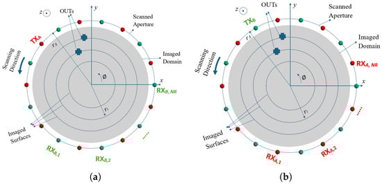
Figure 1.
Cross-section illustration of the proposed imaging system. Small circles show the antennas distributed uniformly along the azimuthal direction. Antennas marked in red and green are connected to switching networks A and B, respectively. Two sample scanning steps are shown: (a) an antenna from switching network A is selected as a transmitter while the receivers are selected from network B; (b) an antenna from network B is selected as a transmitter while the receivers are selected from network A.
In Figure 1a, an antenna () from switching network A (marked in red color) is assigned the role of transmitter, while the receivers ( to ) are selected from network B (marked in green color). Conversely, in Figure 1b, an antenna () from network B acts as the transmitter, with the receivers ( to ) selected from network A.
By implementing this data acquisition configuration at multiple heights , data is acquired using one active transmitter and receiver antennas operating in coordination, forming a virtual cylindrical aperture with radius and height . Thus, the scattered field for each virtual receiver is recorded at angles along the azimuthal direction within 0 to . The process of data collection is performed at frequencies ().
2.1.2. Combination of Electronic and Mechanical Scanning Along the Azimuthal Axis
The physical size of the antennas imposes some limitation on the number of elements used in the array along the azimuthal axis. This, in turn, reduces the number of samples that can be collected along that axis in electronic scanning. To tackle this issue, the number of scanning steps can be increased by adding a few mechanical scanning steps along the direction. At each mechanical scanning step, we repeat the electronic scanning steps discussed in Section 2.1.1.
To clarify further, in this procedure, for each z-position, electronic and mechanical scanning is performed around the aperture. Although electronic scanning is performed with sampling steps of , adding a few mechanical scanning steps and repeating electronic scanning at each step leads us to reach our objective to increase the number of samples by times. As a result, the total number of samples collected at each z-position is calculated as .
2.2. Image Reconstruction Technique
The image reconstruction process is supposed to provide images of objects under test (OUTs) over cylindrical surfaces with radii , where i ranges from 1 to and lies within the interval . For the implementation of the holographic imaging, the approximate point spread functions (PSFs) of the system are measured by placing small point-wise objects (PWO) at cylindrical coordinates of (with reference to Figure 1), one at a time, and scanning the responses over the cylindrical aperture. In total, we measure one PSF function for each imaged surface . According to [20], the total measured scattered field by each virtual receiver antenna and at each frequency can be written as:
where and are convolutions along the azimuthal and longitudinal axes, respectively. The goal is to estimate the contrast functions . For each receiver, the equation above is rewritten across all frequencies as below:
Discrete Fourier transform (DFT) along the axis and discrete time Fourier transform (DTFT) along the z axis are implemented on the equations to transform them to the spectral domain. This allows for forming a system of equations at each Fourier variable pair as shown below that is solved using a standardized minimum norm approach [27]:
where , , and are obtained from , , and when taking DFT and DTFT along the azimuthal and longitudinal directions, respectively; is the identity matrix; and is a vector of ones. In the standardized minimum norm approach, the standardized solution is obtained as:
where is the variance of obtained from:
where is the variance of from a Bayesian point of view, is the diagonal matrix obtained from diagonal elements of , and is
where [. is the Hermitian transpose operation, [. is the Moore–Penrose pseudoinverse, and is the regularization parameter chosen empirically.
Solving the systems of equations in (3) at all pairs provides the images in the spectral domain. Lastly, inverse DFT along and inverse DTFT along z are applied to obtain the reconstructed images in the spatial domain at each imaged surface at .
3. Simulations
This section evaluates the performance of the proposed imaging technique using simulated data obtained from FEKO [28]. Simulations were carried out at two operating frequencies: 1.5 GHz and 1.8 GHz.
With the aim of covering the full circle and considering the size of antennas used in the experiments (discussed later), we used an angular separation of 10 deg between the antennas, which led to having 36 antennas.
In the simulations, all the utilized antennas were z-polarized resonant dipoles. The background medium was characterized by and S/m, while the imaged objects (OUTs) were assigned and S/m. The scattered fields were acquired over a cylindrical aperture with radius mm and height mm.
The imaging was performed on three radial surfaces: 24 mm, 36 mm, and 48 mm. The point spread functions (PSFs) for small 4 mm cuboids placed at these radial distances were simulated. To mimic a realistic environment, additive White Gaussian noise was introduced to the scattered data with a signal-to-noise ratio (SNR) of 30 dB.
Sampling in the longitudinal (z) direction was performed at intervals of , where is the wavelength at the corresponding frequency. The results of the two proposed scanning schemes discussed earlier are presented below for two challenging imaging scenarios.
Figure 2a illustrates the FEKO simulation setup for Simulation Example 1, where three linear cuboidal objects are positioned at radii and . Two of them are placed at with angular positions and , while one is aligned at along the x axis. Table 1 summarizes the parameters for this example.
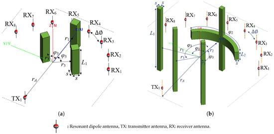
Figure 2.
Simulated models generated using FEKO software. (a) Simulation Example 1: Three cuboid objects (green) positioned on two radial surfaces. (b) Simulation Example 2: Three cuboids and one curved T-shaped object distributed across three radial surfaces.

Table 1.
Values of parameters for Simulation Example 1 shown in Figure 2a.
To further examine the reconstruction performance, we simulate a more complex scenario example depicted in Figure 2b, involving four objects. Simulation Example 2 involves a more complex arrangement with four distinct objects distributed across three radial surfaces, as compared to the simpler configuration in Figure 2a. This example is included to further demonstrate the system’s capability to handle more intricate geometries and object distributions. The reconstruction results from Example 2 provide evidence of the method’s robustness in accurately localizing and resolving multiple targets under more challenging conditions. According to the parameters listed in Table 2, two cuboids are located at , one at , and a more complex structure with two orthogonal arms is placed at .
Table 2.
Values of parameters for Simulation Example 2 shown in Figure 2b.
3.1. Results of Electronic Scanning Along Azimuthal Direction
Instead of employing a stationary array of antennas along the azimuthal direction, the simulation setup involves rotating a transmitter and eight receiver antennas ( with reference to Figure 1) 360 deg around the imaging domain with a step size of , thereby emulating a separation in a fixed array configuration. The chosen number of receiver antennas here is inspired by the work performed in [21], where mechanical scanning was used to collect data along the axis. The angular separation between receiver antennas is deg, consistent with the stationary antenna configuration.
For image reconstruction, the regularization parameter in Equation (11) is chosen empirically, which is a common method (e.g., see [29,30]). To optimize the value of , the quality of the reconstructed images is evaluated using the structural similarity (SSIM) index [31].
In summary, SSIM is computed based on three terms: the luminance term, the contrast term, and the structural term. To find the optimal value of , SSIM is computed for the reconstructed images using the true object’s image as the reference. The true image has a value of 1 at the pixels overlapping the object and 0 elsewhere.
The overall SSIM is computed as the sum of SSIMs calculated for the individual two-dimensional (2D) images at the three radial positions in each image reconstruction process. Therefore, a higher value of total SSIM indicates a greater similarity to the true images.
Please note that this process needs to be performed for at least one set of known objects to optimize the regularization parameter. Here, we perform this for Simulation Example 1 and then use the optimized value for Simulation Example 2. Table 3 shows the variation in total SSIM versus the value of the regularization parameter for Simulation Example 1.
Table 3.
Variation in total SSIM versus the value of regularization parameter for Simulation Example 1.
It was observed that the most acceptable reconstruction quality occurs around . As illustrated in Figure 3a,b, using much higher or lower values such as or results in poor image reconstruction, where the object features are not clearly distinguishable. Thus, we present the results below using .
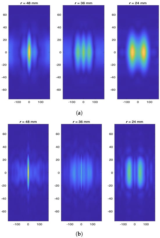
Figure 3.
Image reconstruction results for different values of the regularization parameter which are far from the optimized value for Simulation Example 1, (a) for and (b) for .
Figure 4a presents the reconstructed images for Simulation Example 1. The results indicate successful localization and shape recovery of the targets. It is also evident that image resolution is superior on the outer surface at mm compared to the inner surface at mm. This improvement is attributed to enhanced accessibility and interaction with evanescent components in near-field holography.
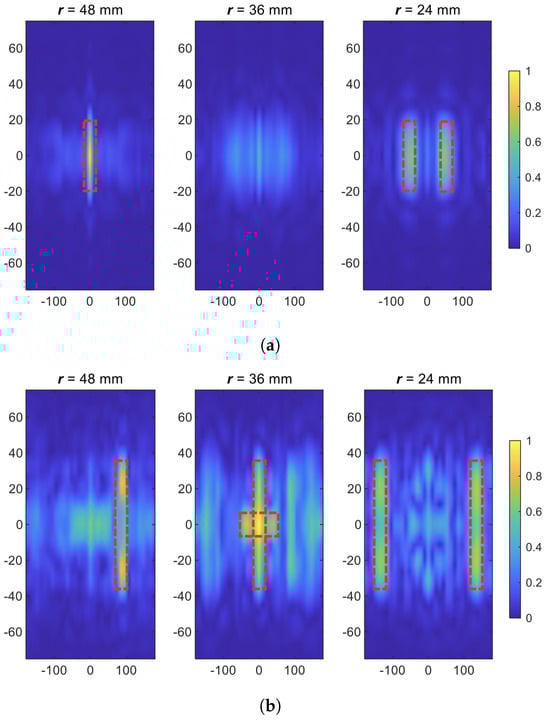
Figure 4.
Reconstructed images for (a) Simulation Example 1 and (b) Simulation Example 2 when 36 samples have been used along the axis and electronic scanning along the azimuthal direction has been performed. Red dashed lines outline the target boundaries. Horizontal axis: (deg); vertical axis: z (mm).
The reconstructed images for Simulation Example 2 are displayed in Figure 4b. The results demonstrate clear localization and differentiation of targets at and . For the object placed at , the contrast is more pronounced along the z axis, aligned with the z-polarized dipole antenna response. As complexity increases, some imaging artifacts and shadowing are observed across adjacent radial surfaces.
3.2. Simulation Results of Electronic and Mechanical Scanning Along Azimuthal Direction
By adding a few mechanical scanning steps and repeating the electronic scanning at each one of those steps, as discussed in Section 2.1.2, the number of collected samples along the azimuthal direction is multiplied by . With the consideration of the experimental setup discussed later, the overall number of 201 samples along the azimuthal direction is calculated and applied in the simulation. Figure 5 shows the simulation results of this data acquisition scheme (201 samples along the axis) for the two examples shown in Figure 2. Comparing the reconstructed images in Figure 4 and Figure 5, it can clearly be observed that the qualities of the reconstructed images are enhanced and two common issues in the reconstruction of images (having object shadows on adjacent planes and spurious artifacts) have been reduced significantly, when a larger number of samples along the azimuthal axis has been acquired.
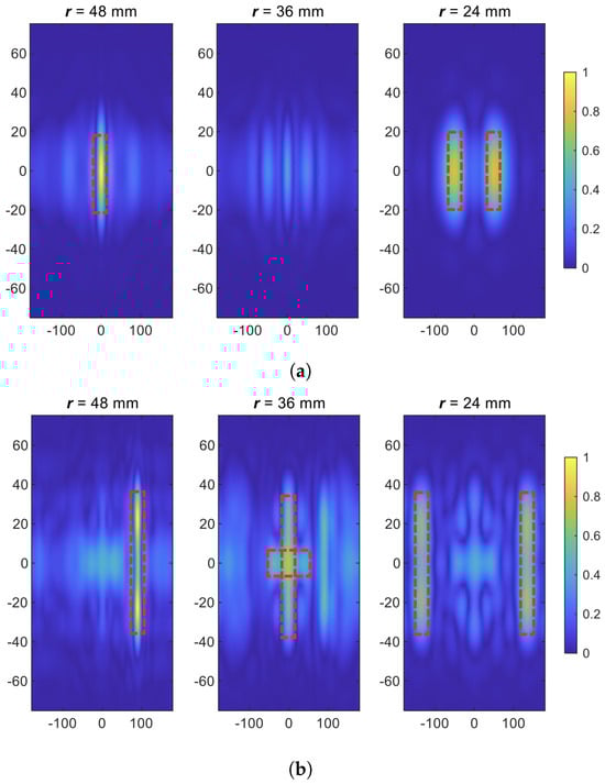
Figure 5.
Reconstructed images for (a) Simulation Example 1 and (b) Simulation Example 2 when 201 samples were used along the axis and electronic and mechanical scanning along the azimuthal direction was performed. Red dashed lines outline the target boundaries. Horizontal axis: (deg); vertical axis: z (mm).
4. Experimental Results
Figure 6 illustrates the block diagram of the proposed imaging system. As shown, it consists of an array of antennas and two switching networks A and B to select the antennas, as discussed in Section 2. The array elements are mini GSM/Cellular Quad-Band antennas from Adafruit [32]. These antennas are a practical, affordable, and technically suitable choice for this microwave imaging system. They operate around 1.5–1.8 GHz, which matches the imaging system’s narrow-band frequencies and allows effective penetration into the glycerine–water medium. Their small size makes it easier to arrange many antennas around a cylindrical setup, achieving higher angular sampling rate. Also, we employ an Anritsu VNA, ShockLine-MS46122B model, for the measurements.
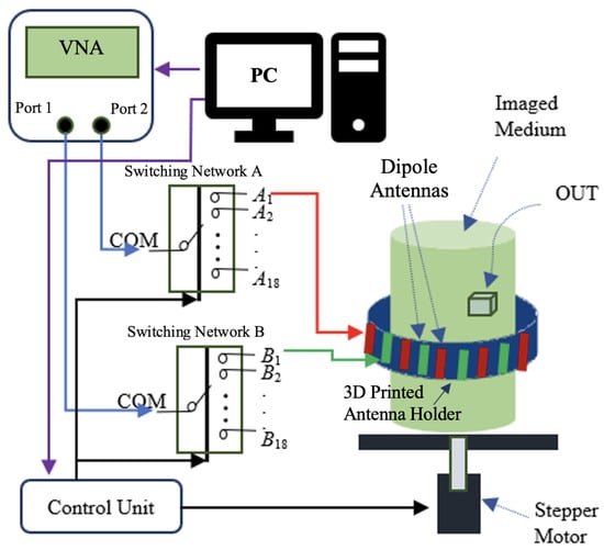
Figure 6.
Block diagram of the imaging system used for measurement. Two ports of the VNA are connected to the common ports of two switching networks. One stepper motor is used for mechanical scanning along the azimuthal direction and another stepper motor (not shown) is used for scanning along the z axis. Dipole antennas (shown by red and green) are connected to the two switching networks A and B, respectively. The objects under test (OUTs) are 3D-printed targets covered by copper sheets.
The scanning setup includes a plexiglass container with a diameter of 125 mm and a height of 200 mm, filled with a liquid consisting of 20% water and 80% glycerin. The liquid has properties of and S/m [33]. This mixture has been chosen due to the similarities of its properties to the averaged tissue properties in biomedical applications [33].
To mitigate the potential influence of the air–liquid interface on the measured signals, the antenna holder was custom designed to tightly accommodate the container and minimize the surrounding gap. This configuration reduces the potential of having interface-related distortions while preserving sufficient leeway to allow mechanical movement of the container along the azimuthal () and longitudinal (z) directions during the scanning process.
The positioning system, which includes an Arduino Uno board, an Arduino motor shield board, and a stepper motor, moves the liquid container along the longitudinal (z) direction. During the measurements, the antenna array remains stationary and is housed in a customized 3D-printed holder, ensuring a gap of 1 mm with the liquid container to allow smooth container movement. We use 36 antennas distributed evenly along the azimuthal direction, covering the full circle. To minimize unwanted cross-coupling between the antennas and reduce the impact of external electromagnetic interference, small microwave-absorbing sheets are placed inside the antenna array holder between adjacent antennas. Specifically, microwave-absorbing sheets with dimensions of 50 mm × 15 mm are inserted into the slots of the holder between each pair of adjacent antennas to reduce mutual coupling. Additionally, the outer surface of the holder is lined with a layer of microwave-absorbing sheet. To further improve shielding, the entire measurement setup is enclosed in a custom-built wooden box, which is also lined with microwave-absorbing material. This layered shielding approach ensures that the measured S-parameters are minimally affected by environmental noise, resulting in more accurate and consistent data for image reconstruction.
Figure 7 shows the variation in the scattering parameters of the antennas. As depicted, Figure 7a shows the variation in the reflection scattering parameter for a sample antenna placed inside the antenna holder and in contact with the liquid container, while Figure 7b shows the variation in the transmission scattering parameter measured for two sample antennas located at the opposite sides of the liquid container. While the figures show the variation over frequencies 1 GHz to 2 GHz, the imaging is performed using the data collected over 1.5 GHz to 1.8 GHz. Figure 7 shows the acceptable performance of the antennas over this frequency range for imaging.
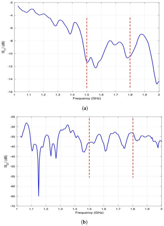
Figure 7.
(a) Variation in reflection scattering parameter for a sample antenna. (b) Variation in transmission scattering parameter for two antennas placed at opposite sides of the liquid container. The red dashed lines indicate the frequency range used for image reconstruction.
The selection of an antenna’s role as transmitter or receiver is controlled by the two switch networks of 1 × 18. Each network is implemented using an Arduino Uno board and three EV1HMC321ALP4E modules, which are RF SP8T switches from Analog Devices. Each network includes a master and two slave modules, controlled by MATLAB through its assigned Arduino Uno board.
Referring to the theory discussed earlier, to perform electronic scanning, the selection of antennas’ roles (transmitter or receiver) is determined such that, while one antenna from a network is selected as a transmitter, the corresponding eight antennas connected to the other network (on the opposite side of the imaged medium) act as receivers. The common ports of the switch networks are connected to the two ports of the VNA, and the transmission scattering parameter is measured for every pair of transmitter () and receiver () antennas () at each scanned height () and measured frequency ().
The assumption of identical antennas is not guaranteed in practice due to fabrication variations, connector mismatches, etc. In the previous work [20], where mechanical scanning was used and each antenna had a fixed role, this issue did not cause significant effects. However, in this work, due to the dynamic assignment of the role of transmitter or receiver to different antennas during electronic scanning, compensation for these variations must be addressed. To overcome this issue, the raw responses of the antennas are pre-processed as
where is the compensated response, is the measured response with the object, and is the response without an object.
The approximation of no-object data is obtained by analyzing the variation in the measured signal along the z-direction. It is assumed that regions with higher signal variation correspond to the positions of the objects, while regions with minimal variation are considered no-object zones. These low-variation regions are used as a reference to approximate the background response.
Figure 8 shows a photo of the experimental setup placed inside a shielding box. The PSFs are collected for objects positioned at radial distances of 20 mm, 35 mm, and 50 mm inside the liquid container, allowing reconstruction of the images on surfaces at these radii. The OUTs are plastic objects covered with thin copper sheets and placed inside the liquid container. Data acquisition is performed over the frequency range from 1.6 GHz to 1.75 GHz with steps of 0.05 GHz.
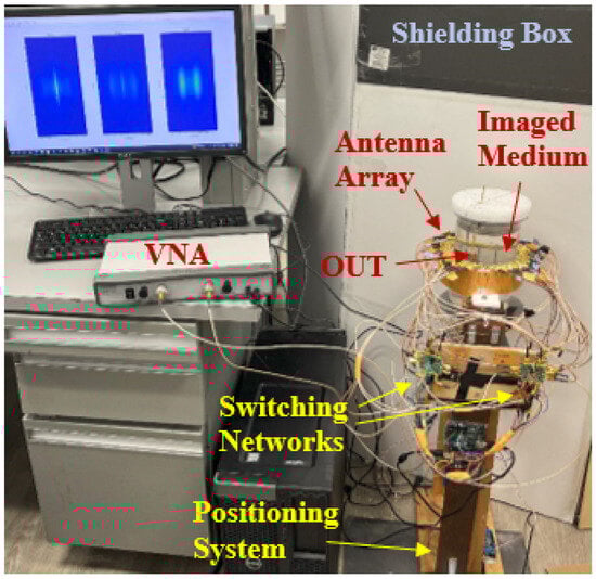
Figure 8.
Photo of the imaging system used for the measurements.
In order to test the proposed scheme in practice, four different measurement scenarios have been performed, as discussed below.
For the first Measurement Example, the OUTs are in the form of cylinders with a height of 50 mm and a diameter of 20 mm, placed at the cylindrical coordinates () of (35 mm, 290 deg, 0) and (50 mm, 180 deg, 0). The mechanical scanning along the z axis is performed from −80 mm to 80 mm with 31 steps. Figure 9a shows the reconstructed images of the positioned objects in the imaged medium. Despite the inevitable presence of environmental interferences and measurement noise, the objects are clearly distinguishable in the images.
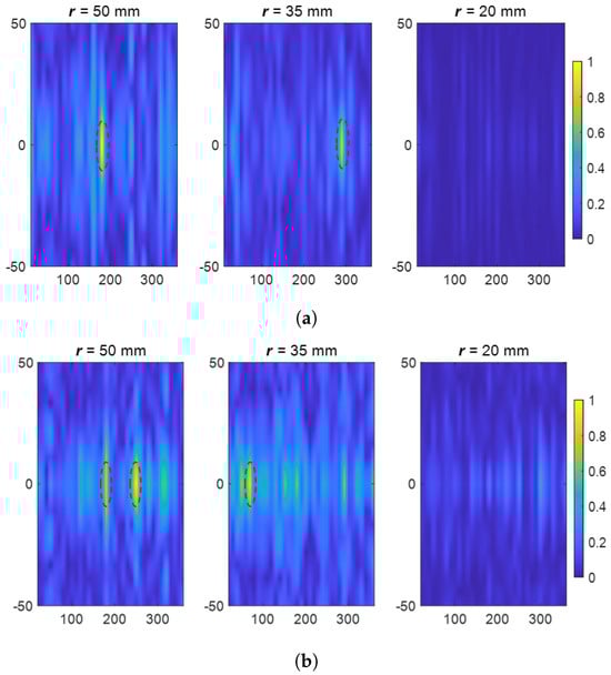
Figure 9.
Measurement results for (a) Measurement Example 1 and (b) Measurement Example 2 when 36 samples along the axis are used. The red dashed lines show the positions of the objects. For all the figures, the horizontal axis represents (deg) and the vertical axis represents z (mm).
For the second Measurement Example, the OUTs are small cuboids with dimensions of 20 mm × 20 mm × 8 mm, placed at the cylindrical coordinates () of (35 mm, 70 deg, 0), (50 mm, 180 deg, 0), and (50 mm, 250 deg, 0). The mechanical scanning along the z axis is carried out from −50 mm to 50 mm in 19 steps. The result of the experiment is shown in Figure 9b. As observed, the objects are reconstructed as expected in their correct positions. In this example, due to the larger number of OUTs, an increase in the level of artifacts is observed, as expected.
In the third measurement experiment, the proposed data acquisition scheme of the combination of electronic and mechanical scanning has been tested and verified practically. With the help of an additional stepper motor that rotates the container along the axis with steps of 1.8 deg, and repeating the electronic scanning at each of these steps, 216 samples are collected along the azimuthal direction. The OUTs are in the form of cylinders with a height of 50 mm and a diameter of 20 mm, placed at the cylindrical coordinates () of (35 mm, −60 deg, 0) and (50 mm, 125 deg, 0). Figure 10a shows the reconstructed images of the two objects. A comparison of the two sets of experimental results in Figure 9 and Figure 10 shows that the increase in the number of samples has a positive impact on the quality of the reconstructed images, helping to reduce the background artifacts significantly.
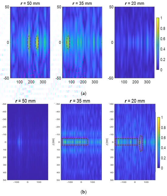
Figure 10.
Measurement results for (a) Measurement Example 3 and (b) Measurement Example 4 when 216 samples along the axis are used. The red dashed lines show the positions of the objects. For all the figures, the horizontal axis represents (deg) and the vertical axis represents z (mm).
To further test the capability of this imaging approach, when using a combination of mechanical and electronic scanning, we perform imaging of a more complicated scenario (Measurement Example 4) in which a narrow and long arc-shaped object is placed on the middle imaged surface (at 36 mm) and along the azimuthal direction and another cuboid object similar to the ones used in the previous example is placed at (20 mm, 90 deg, 0). Figure 10b shows the imaging results for this example. It is observed that the objects are reconstructed in their true positions. However, larger shadows of the arc-shaped object are observed on the adjacent imaged plane at 20 mm. We believe that this degradation of the image quality is due to the fact that this imaging technique is based on the Born approximation [8] which provides better imaging results for smaller and lower-contrast objects (since it ignores multiple scattering between the objects).
5. Discussion
In this section, we provide important discussions related to the comparison of the proposed system with a previously proposed system, selection of the number of antennas and number of samples along the azimuthal direction, and distinguishing the objects in the reconstructed images.
5.1. Comparison of the Two Technique
In near-field microwave holographic imaging, the cross-range resolution of the reconstructed images depends on the portion of measurable evanescent waves, which, in turn, depends on the distance of the object and the antennas and the conductivity of the background medium. Thus, for imaged surfaces closer to the antennas, higher resolutions are expected. Since the distances between the antennas and the imaged surfaces and the conductivity of the background medium in this work are similar to those in [20], the azimuthal and longitudinal resolutions are similar to the ones reported in that work, i.e., 6 mm and 14 mm, respectively. Here, to demonstrate the performance of our imaging system in terms of resolution level, different positioning of objects in the imaged domain are shown in the presented examples. In general, enhancing the number of samples mainly reduces the shadowing level along the range direction.
Furthermore, the data acquisition time depends on the electronic switching time for selecting each pair of transmitter and receiver antennas , mechanical scanning step time , and measurement time of the scattered field (performed by VNA here and by customized data acquisition circuitry in [21]). Thus, in this work the total measurement time is = , while in [21] it is = . Since in general, the mechanical scanning time is much longer than the electronic scanning time due to the required delays in the system to stabilize mechanically, the data acquisition time here is much shorter than the system in [21]. By considering the parameters used in this work and [21], we expect the system to be approximately seven times faster in terms of data acquisition time.
Lastly, the system proposed in this work utilizes more antennas and switching modules to implement the discussed electronic switching scheme. While the system in [21] uses 9 antennas (1 transmitter and 8 receivers) and one SP8T switching module, the proposed system here uses 36 antennas and 6 SP8T switching modules. Thus, the implementation cost of the system here is higher.
Table 4 summarizes the comparison of the proposed system here with the one in [21] as discussed above.
Table 4.
Comparison of mechanical and electro-mechanical scanning techniques.
5.2. Selection of Number of Antennas and Azimuthal Samples for Experimental System
As discussed earlier in the article, the number of samples along the azimuthal direction is determined based on the physical size of the antennas to uniformly cover a full circle (360 deg). In this work, for dense sampling (as per physical constraints) and to maintain a compact array suitable for laboratory setting, an angular spacing of (10 deg) was selected, resulting in (360 deg/10 deg = 36) antennas distributed uniformly around the aperture. Due to space constraints and taking into account the cost of the system (number of utilized antennas and switching networks), it is not favorable to increase the number of antennas further. Thus, to enhance angular sampling, we employed a hybrid approach that integrates mechanical rotation steps along the direction with electronic scanning. Specifically, here the antenna array is mechanically rotated in six incremental steps, each of , and at each step, the full electronic scanning sequence is repeated. The number of mechanical scanning steps was chosen as a compromise between the data acquisition time and quality of the reconstructed images. Consequently, the total number of azimuthal samples becomes at each height, significantly improving angular sampling without increasing the antenna count.
5.3. Distinguishing Reconstructed Objects from Artifacts
To distinguish between reconstructed objects and imaging artifacts, we analyze the brightness levels and spatial consistency across adjacent imaging planes. Genuine objects typically appear with higher brightness intensities and often produce weaker but noticeable shadows on neighboring planes, indicating their volumetric presence. In contrast, artifacts usually exhibit lower brightness and lack continuity or corresponding shadows in adjacent planes, making them visually separable from true object features.
6. Conclusions
In this paper, we introduced a novel near-field holographic microwave imaging system designed to overcome the long data acquisition time of the technique proposed in [21]. By integrating an electronically controlled switching mechanism, the proposed system enables virtual rotation of the antenna array along the azimuthal direction. This significantly reduces the data acquisition time along the azimuthal direction to barely 2 min long at each scanned height. Here, the data collection hardware is implemented in such a way that a space-invariant system is constructed (which is necessary to develop the convolution-based near-field holographic imaging technique), leading to enhanced imaging results. Thus, complex imaging scenarios in which the objects are at multiple range positions can be reconstructed satisfactorily. The methodology was validated through simulations and experiments, demonstrating the system’s capability to accurately reconstruct objects’ images at multiple range positions with enhanced resolution and reduced artifacts. Overall, the system successfully minimizes the common mechanical scanning limitations faced earlier in the systems relying solely on mechanical scanning along the azimuthal direction, such as slow data acquisition time, undesired measurement ripples, unwanted scanning vibrations, etc. This makes it a promising option for various applications demanding fast imaging.
Author Contributions
Conceptualization, R.K.A.; methodology, R.K.A. and M.H.; software, R.K.A. and M.H.; validation, R.K.A. and M.H.; resources, R.K.A.; data curation, M.H.; writing—original draft preparation, M.H.; writing—review and editing, R.K.A. and M.H.; supervision, R.K.A.; project administration, R.K.A. All authors have read and agreed to the published version of the manuscript.
Funding
This research received no external funding.
Data Availability Statement
Data are contained within the article. The data presented in this study can be requested from the authors.
Conflicts of Interest
The authors declare no conflicts of interest.
References
- Zoughi, R. Microwave Non-Destructive Testing and Evaluation; Kluwer: Norwell, MA, USA, 2000. [Google Scholar]
- Ghattas, A.; Al-Sharawi, R.; Zakaria, A.; Qaddoumi, N. Detecting defects in materials using nondestructive microwave testing techniques: A comprehensive review. Appl. Sci. 2025, 15, 3274. [Google Scholar] [CrossRef]
- Nikolova, N.K. Microwave near-field imaging of human tissue and its applications to breast cancer detection. IEEE Microw. Mag. 2011, 12, 78–94. [Google Scholar] [CrossRef]
- Origlia, C.; Rodriguez-Duarte, D.O.; Tobon Vasquez, J.A.; Bolomey, J.-C.; Vipiana, F. Review of Microwave near-field sensing and imaging devices in medical applications. Sensors 2024, 24, 4515. [Google Scholar] [CrossRef] [PubMed]
- Sheen, D.M.; McMakin, D.L.; Hall, T.E. Three-dimensional millimeter-wave imaging for concealed weapon detection. IEEE Trans. Microw. Theory Techn. 2001, 49, 1581–1592. [Google Scholar] [CrossRef]
- Ahmed, S.S. Microwave imaging in security—Two decades of innovation. IEEE J. Microw. 2021, 1, 191–201. [Google Scholar] [CrossRef]
- Sheen, D.M.; McMakin, D.L.; Hall, T.E. Near-field three-dimensional radar imaging techniques and applications. Appl. Opt. 2010, 49, E83–E93. [Google Scholar] [CrossRef] [PubMed]
- Amineh, R.K.; Nikolova, N.K. Fourier-space image reconstruction: The path toward real-time microwave and millimeterwave imaging. IEEE Microw. Mag. 2024, 25, 36–56. [Google Scholar] [CrossRef]
- Tajik, D.; Pitcher, A.D.; Nikolova, N.K. Comparative study of the Rytov and Born approximations in quantitative microwave holography. Prog. Electromag. Res. B 2017, 79, 1–19. [Google Scholar] [CrossRef]
- Tajik, D.; Kazemivala, R.; Nikolova, N.K. Real-time imaging with simultaneous use of Born and Rytov approximations in quantitative microwave holography. IEEE Trans. Microw. Theory Tech. 2022, 70, 1896–1909. [Google Scholar] [CrossRef]
- Zhang, Z.; Liu, H.; Gao, X.; Zhang, Z.; He, Z.S.; Liu, L.; Zong, R.; Qin, Z. Two-Step Iterative Medical Microwave Tomography. Sensors 2024, 24, 6897. [Google Scholar] [CrossRef]
- Slaney, M.; Kak, A.C.; Larsen, L.E. Limitation of imaging with first-order diffraction tomography. IEEE Trans. Microw. Theory Tech. 1984, 32, 860–874. [Google Scholar] [CrossRef]
- Chew, W.C. Waves and Fields in Inhomogeneous Media; IEEE Press: New York, NY, USA, 1990. [Google Scholar]
- Wang, Y.M.; Chew, W.C. An iterative solution of two-dimensional electromagnetic inverse scattering problem. Int. J. Imaging Syst. Technol. 1989, 1, 100–108. [Google Scholar] [CrossRef]
- Chew, W.C.; Wang, Y.M. Reconstruction of two-dimensional permittivity distribution using the distorted Born iterative method. IEEE Trans. Med. Imaging 1990, 9, 218–225. [Google Scholar] [CrossRef]
- Zaeytijd, J.D.; Franchois, A.; Eyraud, C.; Geffrin, J.M. Full-wave three-dimensional microwave imaging with a regularized Gauss–Newton method—Theory and experiment. IEEE Trans. Antennas Propag. 2007, 55, 3279–3292. [Google Scholar] [CrossRef]
- Van den Berg, P.M.; Kleinman, R.E. A contrast source inversion method. Inverse Probl. 1997, 13, 1607–1620. [Google Scholar] [CrossRef]
- Chen, X.; Wei, Z.; Li, M.; Rocca, P. A review of deep learning approaches for inverse scattering problems (invited review). Prog. Electromagn. Res. 2020, 167, 67–81. [Google Scholar] [CrossRef]
- Amineh, R.K.; McCombe, J.; Khalatpour, A.; Nikolova, N.K. Microwave holography using point-spread functions measured with calibration objects. IEEE Trans. Instrum. Meas. 2015, 64, 403–417. [Google Scholar] [CrossRef]
- Amineh, R.K.; Ravan, M.; Sharma, R.; Baua, S. Three-dimensional holographic imaging using single frequency microwave data. Int. J. Antennas Propag. 2018, 2018, 6542518. [Google Scholar] [CrossRef]
- Wu, H.; Amineh, R.K. A low-cost and compact three-dimensional microwave holographic imaging system. Electronics 2019, 8, 1036. [Google Scholar] [CrossRef]
- Ghasr, M.T.; Horst, M.J.; Dvorsky, M.R.; Zoughi, R. Wideband microwave camera for real-time 3-D imaging. IEEE Trans. Antennas Propag. 2017, 65, 258–268. [Google Scholar] [CrossRef]
- Sheen, D.; McMakin, D.; Hall, T.E. Cylindrical millimeter-wave imaging technique for concealed weapon detection. In Proceedings of the 26th AIPR Workshop: Exploiting New Image Sources and Sensors, Washington, DC, USA, 15–17 October 1997; Volume 3240, pp. 242–250. [Google Scholar]
- Sheen, D.M. Sparse multi-static arrays for near-field millimeter-wave imaging. In Proceedings of the 2013 IEEE Global Conference on Signal and Information Processing, Austin, TX, USA, 3–5 December 2013; pp. 699–702. [Google Scholar]
- Wu, H.; Ravan, M.; Amineh, R.K. Holographic near-field microwave imaging with antenna arrays in a cylindrical setup. IEEE Trans. Microw. Theory Tech. 2021, 69, 418–430. [Google Scholar] [CrossRef]
- Manolakis, D.G.; Ingle, V.K. Applied Digital Signal Processing: Theory and Practice; Cambridge University Press: Cambridge, UK, 2011. [Google Scholar]
- Pascual-Marqui, R.D. Standardized low-resolution brain electromagnetic tomography (sLORETA): Technical details. Methods Find. Exp. Clin. Pharmacol. 2002, 24, 5–12. [Google Scholar] [PubMed]
- Altair Feko. Available online: https://altair.com/feko (accessed on 3 March 2025).
- Golnabi, A.H.; Meaney, P.M.; Geimer, S.D.; Paulsen, K.D. Comparison of no-prior and soft-prior regularization in biomedical microwave imaging. J. Med. Phys. 2011, 36, 125–136. [Google Scholar] [CrossRef] [PubMed]
- Golnabi, A.H.; Meaney, P.M.; Paulsen, K.D. Tomographic microwave imaging with incorporated prior spatial information. IEEE Trans. Microw. Theory Tech. 2013, 61, 2129–2136. [Google Scholar] [CrossRef]
- Zhou, W.; Bovik, A.C.; Sheikh, H.R.; Simoncelli, E.P. Image quality assessment: From error visibility to structural similarity. IEEE Trans. Image Process. 2004, 13, 600–612. [Google Scholar] [CrossRef]
- Adafruit Product 1858. Available online: https://www.adafruit.com/product/1858 (accessed on 3 March 2025).
- Meaney, P.M.; Fox, C.J.; Geimer, S.D.; Paulsen, K.D. Electrical characterization of glycerin: Water mixtures: Implications for use as a coupling medium in microwave tomography. IEEE Trans. Microw. Theory Techn. 2017, 65, 1471–1478. [Google Scholar] [CrossRef]
Disclaimer/Publisher’s Note: The statements, opinions and data contained in all publications are solely those of the individual author(s) and contributor(s) and not of MDPI and/or the editor(s). MDPI and/or the editor(s) disclaim responsibility for any injury to people or property resulting from any ideas, methods, instructions or products referred to in the content. |
© 2025 by the authors. Licensee MDPI, Basel, Switzerland. This article is an open access article distributed under the terms and conditions of the Creative Commons Attribution (CC BY) license (https://creativecommons.org/licenses/by/4.0/).