Abstract
Human action recognition (HAR) based on Wi-Fi signals has become a research hotspot due to its advantages of privacy protection, a comfortable experience, and a reliable recognition effect. However, the performance of existing Wi-Fi-based HAR systems is vulnerable to changes in environments and shows poor system generalization capabilities. In this paper, we propose a cross-environment HAR system (CHARS) based on the channel state information (CSI) of Wi-Fi signals for the recognition of human activities in different indoor environments. To achieve good performance for cross-environment HAR, a two-stage action recognition method is proposed. In the first stage, an HAR adversarial network is designed to extract robust action features independent of environments. Through the maximum–minimum learning scheme, the aim is to narrow the distribution gap between action features extracted from the source and the target (i.e., new) environments without using any label information from the target environment, which is beneficial for the generalization of the cross-environment HAR system. In the second stage, a self-training strategy is introduced to further extract action recognition information from the target environment and perform secondary optimization, enhancing the overall performance of the cross-environment HAR system. The results of experiments show that the proposed system achieves more reliable performance in target environments, demonstrating the generalization ability of the proposed CHARS to environmental changes.
1. Introduction
The Internet of Things (IoT) represents a new frontier in information technology, driving significant transformations in various domains of social life, particularly in the area of human–computer interaction (HCI). Within this domain, human action recognition (HAR) has emerged as a particularly prominent and compelling research topic, attracting an ever-growing number of researchers. Currently, research on HAR can be classified into vision-based [1,2], wearable device-based [3], and wireless sensing-based [4,5] methods. However, the first two methods have certain limitations, such as susceptibility to lighting conditions, low privacy, and reduced user comfort, that constrain their practical applications. In contrast, without relying on cameras or wearable devices, wireless sensing technology [6,7,8,9,10] leverages signals such as millimeter wave (mmWave), ultra-wideband (UWB), and Wi-Fi to detect the presence and movement of residents; thus, it has the potential to circumvent the above-mentioned issues. As Wi-Fi signals are highly prevalent in indoor settings, they hold immense potential for future HAR applications, especially considering the widespread and continuously increasing use of home wireless networks.
HAR technology based on Wi-Fi signals recognizes actions by analyzing the effects of different actions on wireless signal propagation. Early Wi-Fi-based HAR research relied on the received signal strength indicator (RSSI) [11,12], a coarse-grained indicator for evaluating the quality of communication links to recognize actions. In order to better reflect the impact of human behavior on Wi-Fi signals, the use of channel state information (CSI) for action analysis [13,14,15,16,17,18,19,20,21,22] is becoming mainstream, as it can be easily extracted from commercial wireless network interface cards (NICs). As a more fine-grained indicator, it can describe more propagation characteristics of multipath superposition signals received by the receiver, including multipath delay, fading, and other related information. Extracting effective features from these signals disturbed by actions is the key to reliable HAR. Currently, with the rise of deep learning technology, deep learning networks [23,24,25,26] have been widely utilized and have achieved great success in HAR tasks due to their powerful feature extraction capabilities. By collecting action data in an environment to train the recognition network, high recognition performance can be achieved in that environment.
Nevertheless, there are still some challenges. In certain cross-environment action recognition scenarios, the pre-trained network from the source environment often struggles to achieve satisfactory performance in the target environment. This difficulty arises because variations in the perception environment lead to changes in the signal propagation path, which makes the multipath superposition signal received by a receiver in different environments exhibit different characteristics, even when the same action is performed. This shift in the distribution of action data between the source environment and the target environments prevents a network trained solely in the source environment from effectively fitting action features in the target environment, leading to a decline in target-environment recognition performance. However, it is unrealistic to perform the entire data collection, labeling, and network retraining again in the target environment to ensure reliable HAR performance. Due to labor constraints, target environments often only provide a small number of, or even unlabeled, samples. Therefore, achieving reliable cross-environment recognition in this case is one of the urgent challenges that HAR needs to address.
To solve this problem, this paper proposes a two-stage cross-environment human action recognition system (CHARS). First, in order to narrow the gap between the action features of the source environment and the target environment without using any action labels in the target environment, an adversarial network is designed. By introducing a feature distance discriminator in the recognition network and adopting a maximum–minimum learning strategy, the feature extractor in the recognition network is guided to map the action data in the source and target environments to a common latent space, in which the features are more independent of environmental variations, which is conducive to improving the recognition performance of the recognition network in the target environment. On this basis, inspired by the theory of semi-supervised learning, a self-training strategy is designed to further extract action recognition information from the target environment, optimizing the network by utilizing the selected training samples and their pseudo-label information in the target environment. Consequently, the network is expected to achieve better HAR performance in the target environment. Extensive experiments are conducted to verify the effectiveness of this system, and the action recognition performance in both the source environment and the target environment is reported. The experimental results show that the CHARS achieves reliable recognition performance across a variety of cross-environment HAR scenarios.
In summary, the main contributions of this study are as follows:
- We develop an adversarial network that guides the recognition network to map actions from different environments to the environment-invariant feature latent space through a max–min learning strategy, thereby narrowing the feature distance of actions in the source environment domain and the target environment, which is beneficial for HAR performance in the target environment.
- We develop a self-training strategy to further extract action recognition information from the target environment and, through semi-supervised network optimization, improve action recognition performance in the target environment.
- We conduct extensive experiments in different environments and report the recognition accuracy in both the source and target environments, which demonstrates the effectiveness of the proposed system.
The remainder of this paper is organized as follows. We introduce related works on the cross-environment HAR task in Section 2. Section 3 presents preliminary background knowledge and the challenges of the cross-environment action task. The detailed methodology of our CHARS is described in Section 4. Then, we implement the experiments and evaluate HAR performance in Section 5. The overall conclusions of this work are presented in Section 6.
2. Related Works
Early wireless Wi-Fi signals-based human action recognition methods usually used RSSI for analysis. PAWS [11] uses an online activity recognition architecture based on RSSI, and WiGest [12] constructs mutually independent gesture families for gesture recognition without the effort of training. As coarse-grained information, RSSI has certain limitations in high-precision recognition. With the development of commercial NICs, CSI, as an indicator with richer communication link information than RSSI, is extracted and gradually dominates the recognition task. Early CSI-based action recognition computed the statistical features of time-frequency signals and utilized machine learning methods to achieve recognition. Tahmid et al. proposed a CSI-based action recognition system called WiHACS [16], which extracts a series of statistical features, including mean, skewness, kurtosis, and normalized entropy, and uses a multi-class support vector machine (SVM) for action recognition. Wang et al. [17] exploited histogram distribution for analysis in their home activity monitoring system E-eyes. Pu et al. [18] achieved gesture recognition by capturing the Doppler profile of gestures and pattern matching. Nowadays, the development of deep learning and computational capacity has further encouraged many researchers to design deep learning networks to achieve feature extraction and action classification. Ref. [19] demonstrated the superior performance of a deep learning-based method compared to a machine learning-based method with handcrafted features. Refs. [23,27] proposed a convolutional neural network (CNN)-based HAR network. Ref. [28] developed a CNN and long short-term memory (LSTM) combined network for activity recognition. Ref. [29] proposed a data augmentation method and transformer-based HAR network. Ref. [30] designed a multi-scale convolution transformer-based network for HAR. All of these methods achieved outstanding performance in HAR. However, most of these works did not consider the effects of environmental changes. Next, we provide a thorough overview of the existing literature on Wi-Fi-enabled cross-environment HAR, in which we classify the proposed solutions into three main categories, including signal processing-based, transfer learning-based, and domain adaptation (DA)-based methods, and discuss their main features and potential limitations.
Signal processing-based methods focus on examining the intrinsic properties of input signals to identify robust features that persist across diverse environments. By leveraging these features, a cross-environment HAR model can be effectively trained and optimized. One approach used in signal processing-based methods to isolate these features involves the use of advanced signal processing techniques to analyze received Wi-Fi signals. For instance, Ref. [20] used commercial Wi-Fi devices to estimate Doppler shifts from channel frequency response (CFR) data, enabling the accurate recognition of activities across different individuals and environments. Zhou et al. [31] employed the low-rank and sparse matrix decomposition technique to separate input signals into background noise and sparse information specifically related to actions. Widar3.0 [32] calculates body-coordinate velocity profiles (BVPs) from Doppler frequency shifts, facilitating the extraction of position-robust features. Another approach adopts statistical and pattern recognition techniques for feature extraction, reducing the dimensionality of the feature space and pinpointing the most relevant features. For example, Wu et al. [33] explored the use of opposite robust principal component analysis (or-PCA) to capture the correlation between human activities and CSI changes while minimizing the impact of environmental factors on correlation extraction. However, signal processing-based methods often require substantial expertise for effective implementation. Manual signal parameter selection can unintentionally result in the loss of essential signal information and increased system design complexity. As a result, these methods may exhibit limited adaptability and may not be ideally suited for recognizing human actions in unpredictable environments.
As deep learning techniques rapidly advance, transfer learning has emerged as the primary approach to address cross-environmental challenges in Wi-Fi-enabled HAR. This method leverages pre-trained models, initially designed for specific environments, and refines them for new contexts. Fine-tuning, a simple yet effective transfer learning technique, plays a crucial role in achieving generalization across diverse environments. By utilizing a limited number of manually labeled samples from the new environment, fine-tuning optimizes model parameters to better align with the data distribution in the new context. These models typically employ state-of-the-art architectures, such as CNNs and LSTMs. For instance, Ref. [34] developed a recognition model incorporating CNN and LSTM architectures, leveraging a small set of samples from the new environment to fine-tune the model. Few-shot learning can be seen as a special type of transfer learning. Refs. [21,22] introduced a one-shot learning approach for HAR using a matching network with enhanced channel state information (MatNet-eCSI), addressing the challenges of requiring large sample requirements and adapting to new environments. Nevertheless, transfer learning-based methods heavily depend on the availability of annotated data, especially when deploying the model in previously unencountered scenarios. This reliance may restrict their applicability in situations where labeled data are unavailable.
DA is indeed an alternative approach to transfer learning for cross-environment HAR [35,36,37], as it does not necessarily require labeled data in the new environment. The primary reason for this is its focus on minimizing the distribution discrepancy between the source and target domains, enabling the model to generalize better to the new environment without the need for fine-tuning using labeled samples. This objective is achieved through techniques such as adversarial training, which emphasizes learning domain-invariant features, rather than relying on labeled data from the new environment. For instance, EI [36] is a model that includes an additional domain discriminator to learn domain representations by maximizing the domain label prediction loss, thus eliminating domain-related features. Han et al. [37] developed a multi-kernel maximum mean discrepancy (MK-MMD)-based deep adaptation network for domain-invariant feature learning. Despite not requiring labeled data in the target domain, existing DA-based methods often rely on sufficient unlabeled data for effective model adaptation. In scenarios with notable distribution differences between the source and target domains, the learned features may still display a bias toward the source domain. Under such circumstances, especially when only a limited amount of target domain data is accessible, this problem can be amplified, resulting in decreased performance. In this paper, we propose the CHARS, a system that employs a robust two-stage optimization method consisting of adversarial training and self-training, making it more adaptable in handling target environments with unannotated data. The proposed adversarial learning strategy aims to reduce the distribution discrepancy of action features across different environments. At the same time, the proposed self-training strategy aims to further extract action recognition information from the target environment, improving action recognition performance. This allows it to achieve better cross-environment recognition performance, even when samples are relatively limited.
3. Preliminaries
This section begins by presenting the background knowledge of CSI for Wi-Fi-enabled data collection platforms. Subsequently, a concise overview of the experimental measurements is provided. Building upon this, we conduct a detailed analysis of the collected data to thoroughly examine the challenges associated with cross-environment HAR tasks.
3.1. Channel State Information
In a typical indoor Multiple-Input Multiple-Output (MIMO) and Orthogonal Frequency Division Multiplexing (OFDM)-based wireless Wi-Fi signal transmission scenario, the signal transmitted from the transmitter often undergoes complex reflection, scattering, and diffraction due to the presence of environmental obstacles, resulting in a multipath superimposed signal at the receiver. Consequently, channel state information (CSI) plays a critical role by providing detailed information about the channel properties, allowing for a precise description of the signal propagation process described above. Assuming a transmitter with antennas and a receiver with antennas, the signal transmission process can be mathematically modeled as
where y and x represent the received and transmitted signals, respectively; is the noise; and H is a complex CSI matrix. The CSI at a certain time t can be expressed as
where N represents the number of subcarriers for each pair of antennas, , where and indicate the amplitude and phase of the CSI for the k-th subcarrier, respectively. Furthermore, the CSI matrix obtained from T frames can be denoted as
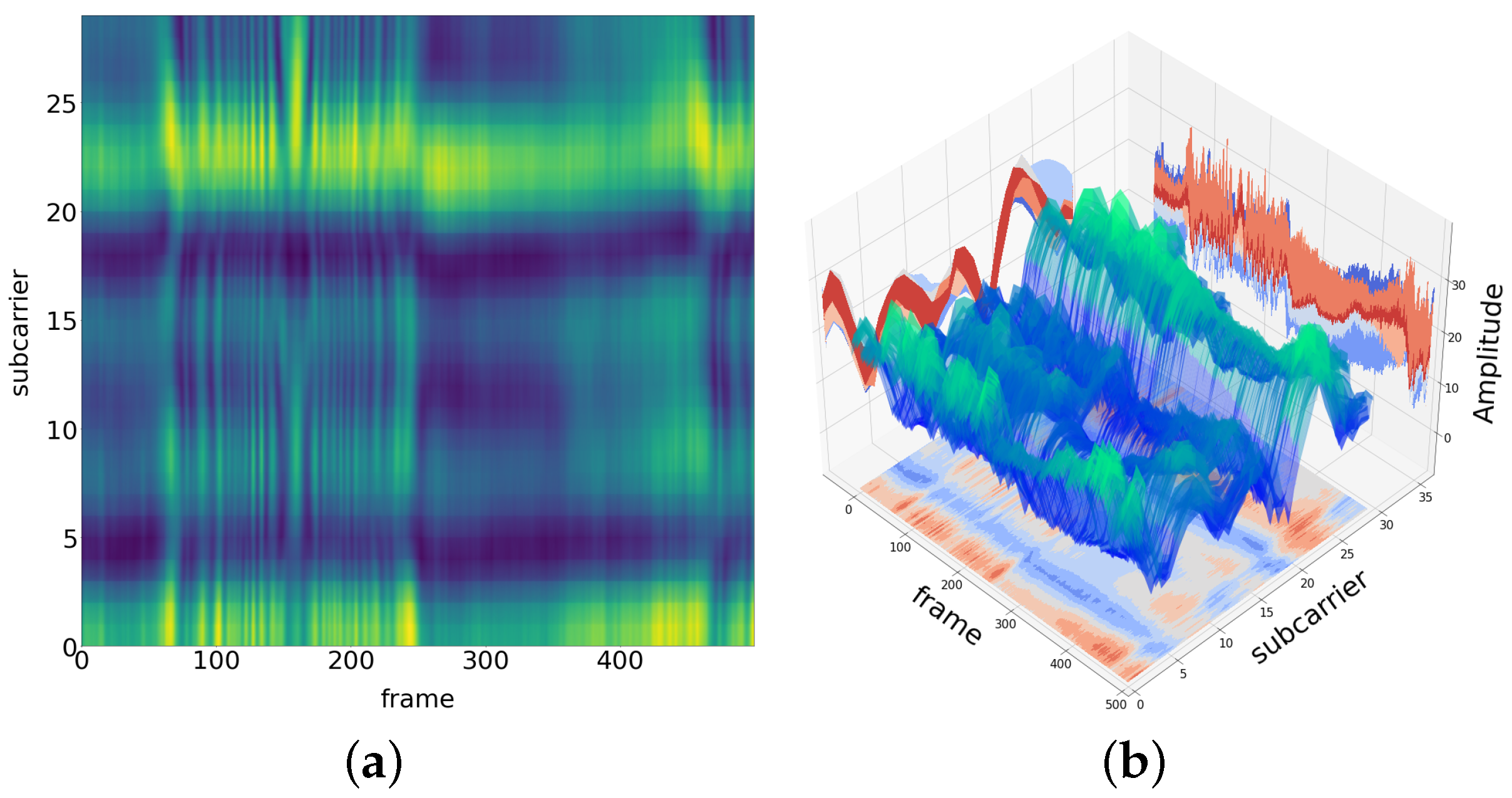
Figure 1 shows the two-dimensional (2D) and three-dimensional (3D) CSI amplitude maps of an example Wi-Fi signal in an indoor environment. The subcarrier axis represents the 30 subcarriers collected from one pair of transmitting and receiving antennas. The frame axis represents the data packets received within 2.5 s. The amplitude axis represents the amplitude magnitude of the CSI.

Figure 1.
(a) 2D CSI amplitude map of a signal in an indoor environment, the yellower the color, the larger the amplitude, and the greener the color, the smaller the amplitude. The two coordinate axes represent the frame and subcarrier. (b) 3D CSI amplitude map of a signal in an indoor environment. The three coordinate axes represent the frame, subcarrier, and amplitude.
3.2. Experimental Measurements
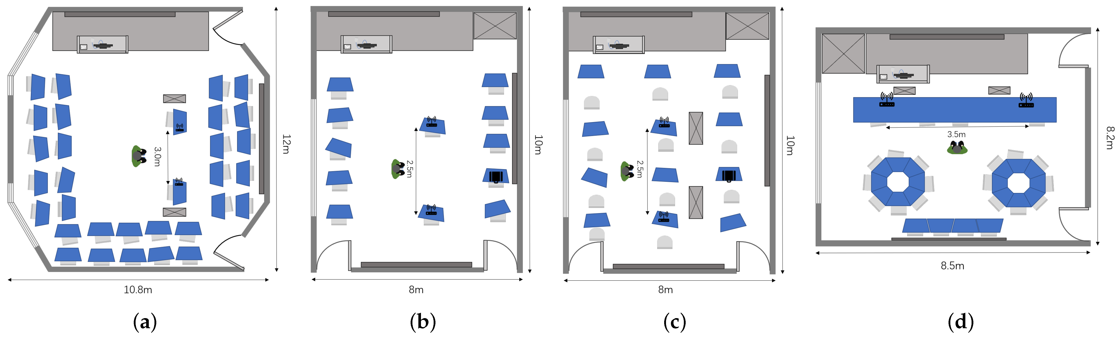
To evaluate the performance of the developed system, particularly its accuracy in recognizing various actions performed across different environments, measurements were conducted in four different environments: , , , and . These environments were chosen due to the diverse degrees of layout differences they exhibit. For example, and correspond to two separate configurations within the same room (10 × 8 m2), resulting in relatively smaller environmental disparities. Conversely, (10.8 × 12 m2) and (8.2 × 8.5 m2) are entirely different rooms, leading to more significant differences in environmental characteristics when compared to and . Consequently, these layouts allowed us to test the system’s ability to effectively address challenges arising from different domain discrepancies. The detailed data collection layouts are illustrated in Figure 2. For all measurements, two PCs installed with Intel 5300 NICs served as the Wi-Fi transmitter and receiver, and the distance between the transceivers remained unfixed. Both of them were equipped with three omni-directional antennas. The transceivers operated in IEEE 802.11n AP mode at a 5 GHz frequency band with a 20 MHz bandwidth, and the transmit power was 15 dBm. CSI tools [38] were utilized to acquire raw CSI data. The sensing target was located on the mid-perpendicular line of the straight-line distance between the transceivers, around 0.5m away from the transceiver. As 30 subcarriers for each – pair could be obtained with CSI Tools, there were subcarriers collected in total. The data sampling rate was set to 200 packets per second, and the sensing duration for each action was 5 s.
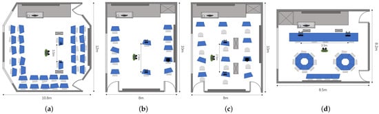
Figure 2.
Experimental environmental layouts: (a) , (b) , (c) , and (d) . Notably, and correspond to two distinct configurations within the same room, while and represent separate rooms.
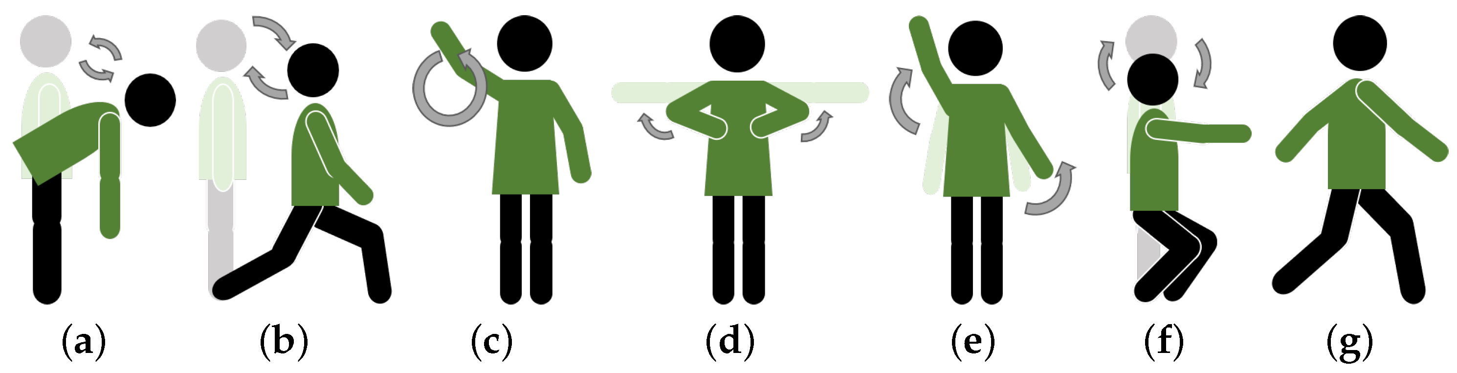
Considering the potential applications, including fitness and Virtual Reality (VR) gaming, which involve body movements, as well as smart device control applications involving upper-limb movements, seven common fitness activities and arm movements were used in this paper for HAR, including (a) standing forward bend (SFB), where one bends forward from a standing position, letting the arms hang naturally while stretching the back and hamstrings; (b) lunge (LG), where one steps one leg forward while lowering the hips until both knees form a 90-degree angle, keeping the torso upright; (c) one-arm circle (O), where one extends one arm to the side and draws circles in the air with the hand while keeping the arm straight; (d) chest expansion (CE), where one extends both arms to the sides at shoulder height and pulls them back while opening the chest, then returns to the starting position; (e) arm stretching (ST), where one extends the arms upward or outward to stretch the muscles and relieve tension; (f) half-squat (HS), where one lowers the body by bending the knees while keeping the back straight, stopping when the thighs are parallel to the ground; and (g) walking (WK), where one moves forward by alternating steps with both feet, maintaining a steady pace. The process details of each action class are illustrated in Figure 3. Given that we primarily aimed to investigate the challenges of cross-environment HAR, we recruited a volunteer and asked him to stand between the transmitter and receiver in each indoor room. While the transmitter sent signal packets to the receiver, the volunteer was instructed to perform all seven action classes. For each class of action, 50 CSI samples were recorded in each environmental layout. The measurements were recorded over several days.

Figure 3.
Seven common fitness action and arm movements, including (a) standing forward bend (SFB), (b) lunge (LG), (c) one-arm circle (O), (d) chest expansion (CE), (e) arm stretching (ST), (f) half-squat (HS), (g) walking (WK).
3.3. Data Analysis
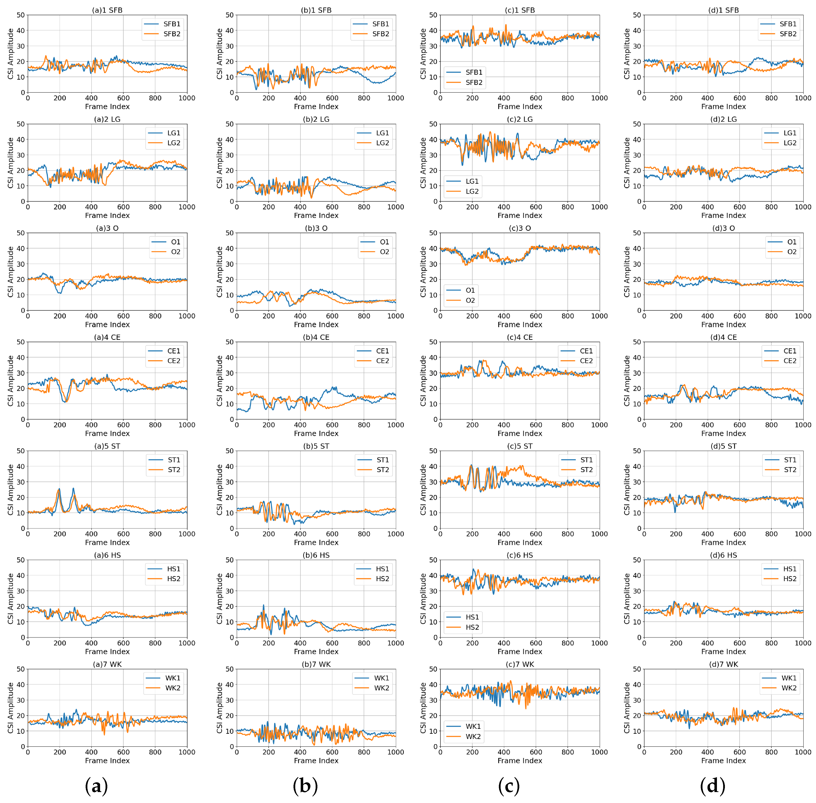
To illustrate the challenge of cross-environment HAR tasks, we provide a comprehensive analysis by visualizing one of the CSI subcarriers (the 4th out of 270). Figure 4 displays the denoised CSI data for each action measured across different environments for clarity, with the y-axis indicating the amplitude value and the x-axis representing the frame number, which can alternatively be described as the length of the received packets. Due to the different durations of each action, the number of frames corresponding to action fragments within the CSI samples also varies. As such, it is essential to precisely identify both the starting and ending points of action segments within each CSI sample and subsequently utilize the extracted fragments for HAR. This paper employs an action segmentation algorithm for action segmentation within the developed CHARS framework, which is described in the next section.
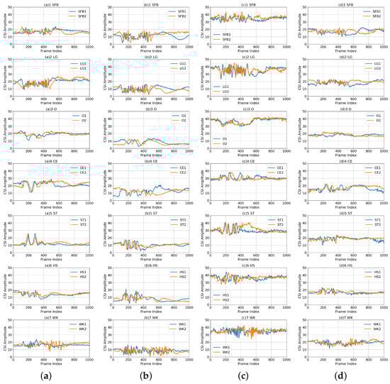
Figure 4.
CSI amplitude measurements on the 4 subcarrier. (a–d) Comparisons between different actions (i.e., SFB, LG, O, CE, ST, HS, and WK) in four environments (i.e., (a) , (b) , (c) , and (d) ). Notably, the digits 1 and 2 in the legend indicate two distinct samples belonging to the same action (e.g., SFB 1 and SFB 2 denote two samples measured within the action class SFB).
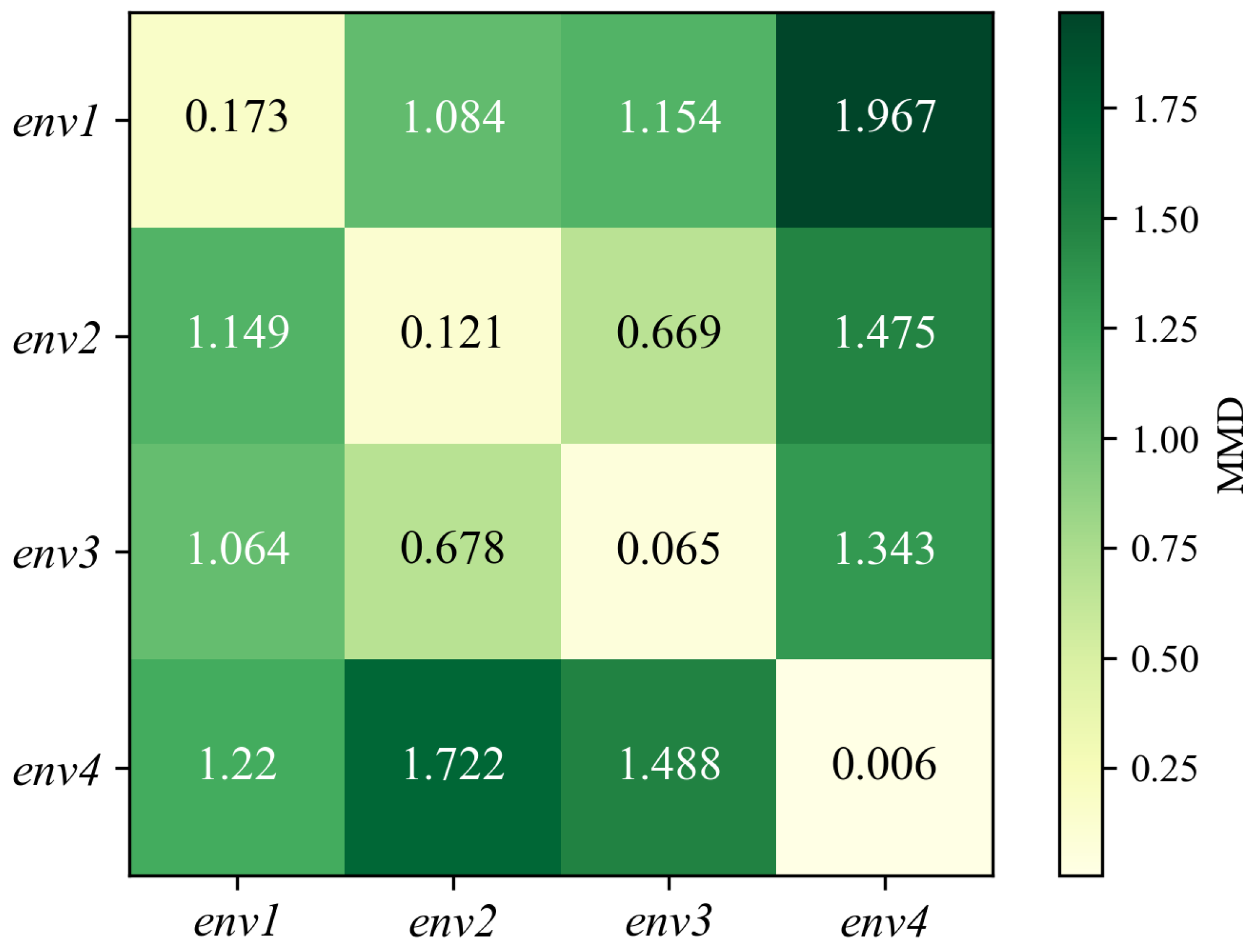
In the figures, it is also noticeable that when actions are executed within the same environment, the CSI amplitudes for identical activities exhibit similar trends, which vary distinctly for distinct activities. This suggests that it is possible to recognize different activities based on their unique patterns of CSI amplitudes. Conversely, when actions are performed across various environments, the measured CSI amplitudes of the same human activity exhibit different patterns. This cannot guarantee good performance of cross-environment HAR. To better analyze the changes in the signal transmission paths caused by environmental variations, the maximum mean discrepancy (MMD) distance is used to quantify data distribution differences between various environments:
where and are randomly selected samples, and and denote the number of samples in different environment sets, respectively. The function represents a kernel function that maps the original data into a Reproducing Kernel Hilbert Space (RKHS) . Figure 5 visualizes the pairwise MMD between distributions from different environments. Note that a larger metric value in the matrix indicates a greater disparity between the respective environments. The data distribution differences are smaller within the same environment, while they are larger across distinct environments. This article proposes a two-stage optimization method in the CHARS to achieve reliable HAR performance in the target environment.
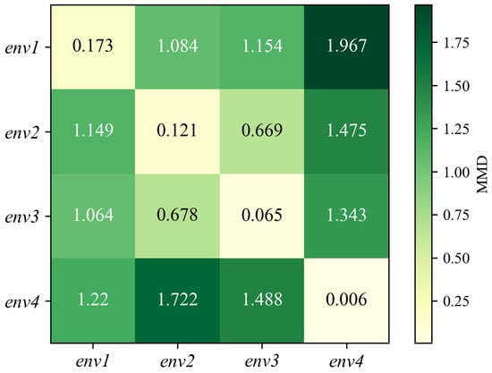
Figure 5.
MMD distance of action samples between each environment.
4. Methodology
In this section, we provide a detailed introduction to the proposed CHARS. We first present a system overview. Then, the data preprocessing method is described. Finally, the two-stage optimization action recognition method is presented.
4.1. Overview of CHARS Framework
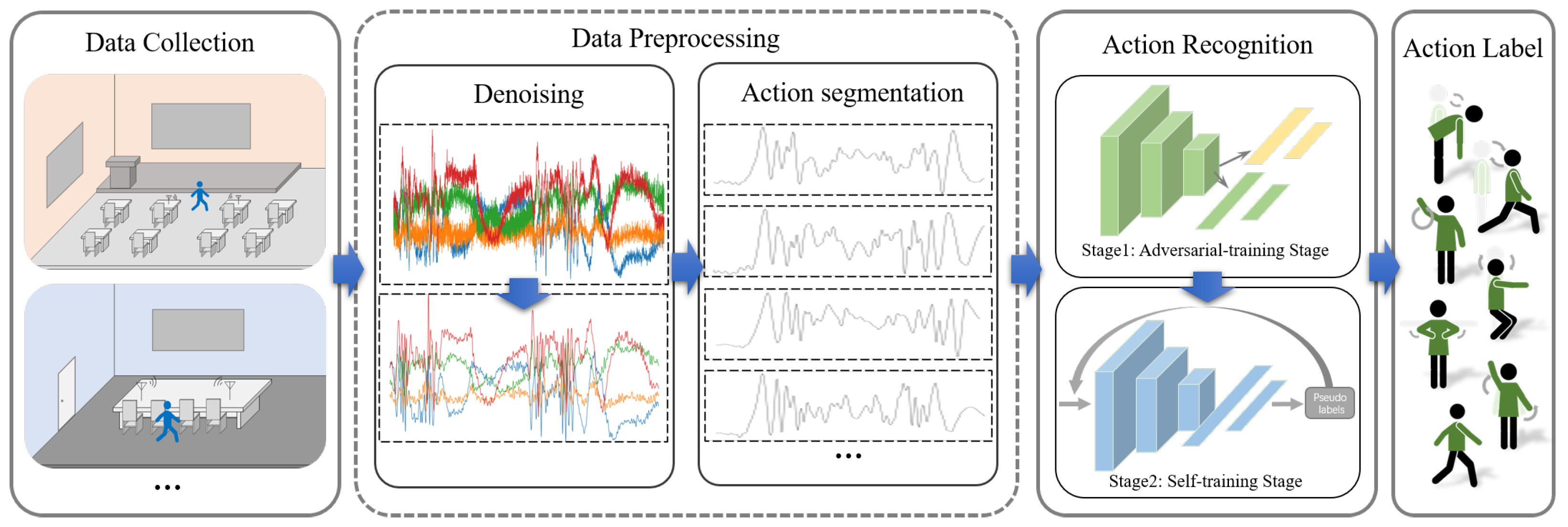
The CHARS framework is shown in Figure 6 and consists of three modules: data collection, data preprocessing, and action recognition.
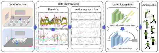
Figure 6.
CHARS framework, which consists of three modules: data collection, data preprocessing, and action recognition.
Data Collection: In the data collection phase, the human action CSI data is collected in different environments. There is a pair of Wi-Fi transceivers placed at a certain distance in each indoor environment. The volunteer is required to perform different actions between the transceivers. The details are described in Section 3.
Data Preprocessing: This module consists of two stages: denoising and action segmentation. The denoising operation eliminates noise interference during the data collection process, which is more conducive to subsequent data analysis. For the action segmentation stage, we develop an action segmentation algorithm to divide the denoised CSI amplitude data into short CSI action fragments for recognition.
Action Recognition: This module is the core part of the CHARS and consists of two stages. The first stage is the adversarial training stage, where we design an adversarial network and introduce a maximum–minimum learning strategy. This guides the recognition network to map actions from both the source and target environments to a more environment-invariant feature space, thereby enhancing the recognition performance of the recognition network in the target environment. In the second stage, we further introduce a self-training strategy to fully extract the pseudo-label information from actions in the target environment, enabling semi-supervised optimization of the recognition network and further improving HAR performance in the target environment.
4.2. Data Preprocessing
4.2.1. Data Denoising
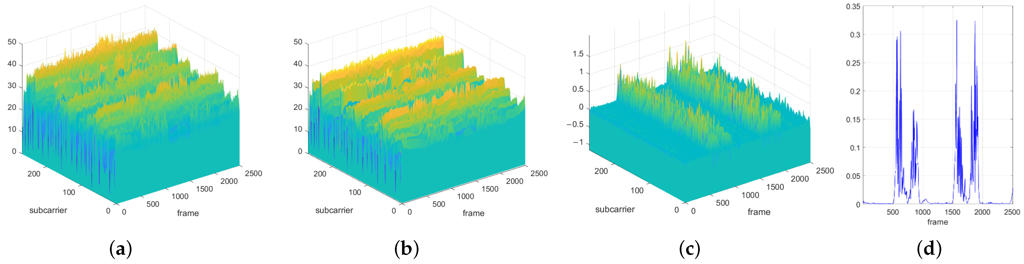
In the data collection process, in addition to the signal fluctuations caused by the action, the noise in the equipment and environment also causes serious interference to the signal. This high-frequency noise has an impact on the subsequent signal analysis. Therefore, it is very important to denoise the raw CSI data. Based on this, this paper uses a fifth-order Butterworth low-pass filter in the proposed CHARS to remove the high-frequency noise from the raw CSI that does not belong to the action component. The raw data and the denoising result are shown in Figure 7a and Figure 7b, respectively.
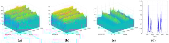
Figure 7.
(a) Raw CSI data. The yellower the color, the larger the amplitude, and the greener the color, the smaller the amplitude. (b) Denoised CSI data derived from the raw CSI data. (c) The waveform of data , obtained after performing the differential operation on the denoised CSI data over the time domain. (d) The waveform of data , representing the variance of over the subcarrier domain.
4.2.2. Action Segmentation
Another key issue in data preprocessing is action segmentation. Some existing methods use additional timestamps for action segmentation, which increases the workload and is inconvenient [23,28]. To address these problems, we propose a dynamic data detection method (DDDM) to perform action segmentation automatically, inspired by the observation that actions impact subcarriers’ fluctuations to varying degrees. The steps in the DDDM algorithm are as follows:
Step 1: To remove the static component of the CSI data and observe the fluctuations influenced by actions more explicitly, the first step of the DDDM performs a differential operation on the CSI over the time domain, which can be expressed as
where is the amplitude of the denoised , as mentioned in Section 3.1, and K is the number of subcarriers. The result of is shown in Figure 7c. We can observe that the data changes flatly when no action is performed. However, once someone acts, the signal waveform fluctuates more drastically over time and the subcarrier domains.
Step 2: With the observation above, the second step of DDDM calculates the variance of over the subcarrier domain at each frame. This process can reflect the data fluctuations without time delay:
where and K is the number of subcarriers. The result after this operation is presented in Figure 7d.
Step 3: A sliding window is applied to further process the data () to identify the start and end points of the action fragments. As the sliding window moves through with a step size of 1, the percentage of data packets that exceed the set threshold relative to all packets within the window is calculated. If this percentage exceeds the threshold p, the packets within the sliding window are classified as part of the action fragment. Specifically, to ensure the effectiveness of action fragment detection across all environments, the threshold is empirically set to four times the mean value of in the static environment, and the percentage threshold p is set to 30%. The size of the sliding window in this work is set to 50 frames. Once the sliding window has covered the entire dataset, all the start and end points of the action fragments are determined. When the sliding window passes through the entire data stream , we can divide all the data into action parts and static parts. Based on the time frames of all the action parts, we then determine the starting and ending points of all the action segments.
Step 4: To compress the data and improve system efficiency, we apply PCA [39] on the denoised CSI data to obtain the one-dimensional (1D) CSI data and then segment the dimensionality-reduced CSI to extract individual action fragments based on the start and end points obtained from the actions in Step 3.
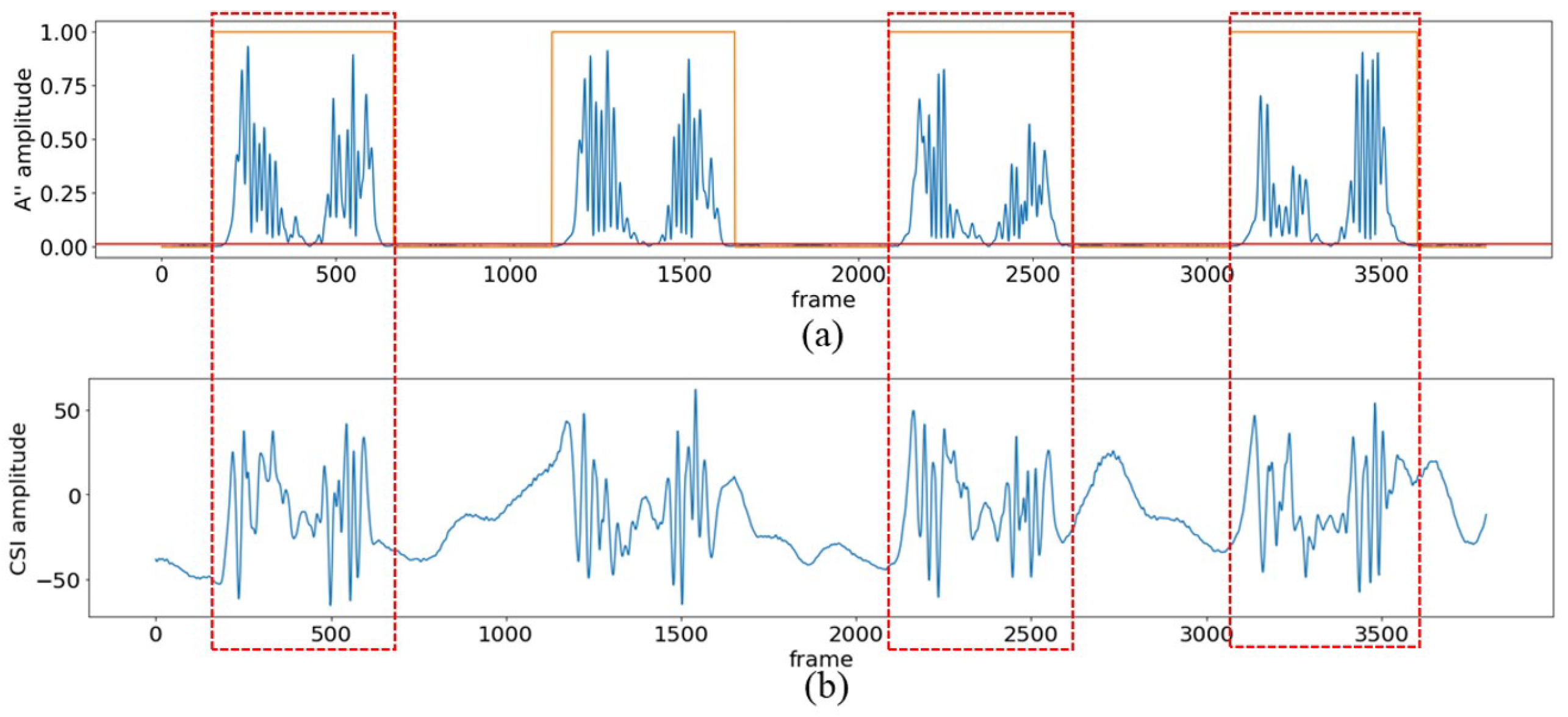
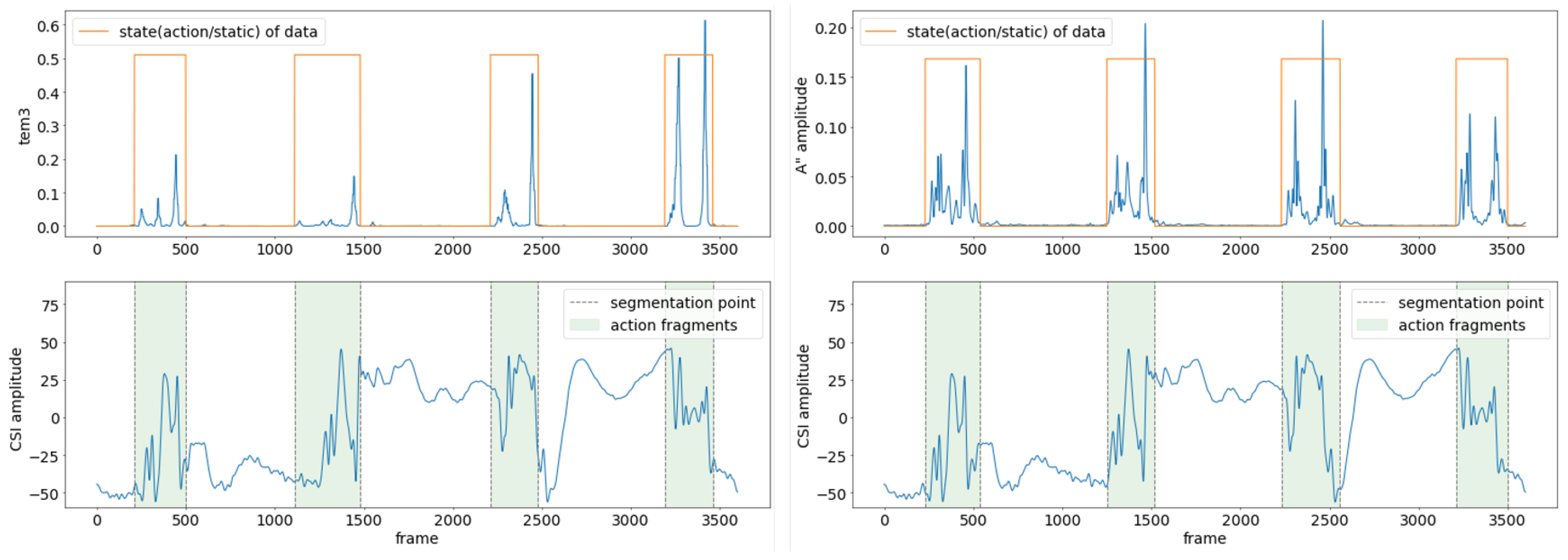
The action segmentation effect of the DDDM algorithm is shown in Figure 8, using the action ’standing forward bend (SFB)’ as an example. In Figure 8a, the blue line denotes . The red line is the threshold of the action. The orange line indicates the data states through Step 3, where a high level means the data corresponds to the action fragment, and a low level means the data belongs to the static fragment. The red dotted boxes in Figure 8b show the action fragments corresponding to the detected starting and ending points. We can observe that in the static phase, is very stable and close to 0, and in the action phase, fluctuates violently, which is consistent with the intensity of the action.
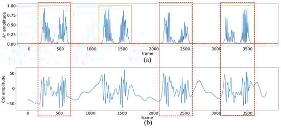
Figure 8.
Data segmentation effect of the DDDM algorithm. (a) The waveform of , which reflects the state of the CSI data shown in (b). (b) The waveform of the dimensionality-reduced CSI data; the data clips in the red box represent the action fragments.
Figure 9 compares the results of the segmentation algorithm (AACA) in [40] with our method (DDDM). In detail, AACA processes the action data over the time domain several times, such as computing the variances of the sliding window over the time domain, which leads to a time offset of the data state to a certain extent. Additionally, AACA ignores the chronological order of the action data and determines the data state of the current packet by using the data of future time in the sliding window, which is unrealistic and limits its application. In contrast, our method avoids the time offset of the data state and considers the chronological order at the processing stage, which can achieve action segmentation better.
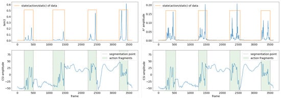
Figure 9.
Data segmentation effect of AACA in [40] (left) and DDDM (right).
4.3. Action Recognition
Action recognition in the CHARS consists of two stages: adversarial training and self-training. The adversarial training stage aims to map action samples from both the source and target environments to a latent space where action features are more independent of environmental changes. This is achieved through a carefully designed adversarial network and the maximum–minimum learning strategy, without relying on any action label information from the target environment. In the self-training stage, a strategy is proposed to extract pseudo-label information from actions in the target environment and implement semi-supervised secondary optimization, further improving HAR performance in the target environment.
4.3.1. Adversarial Training Stage
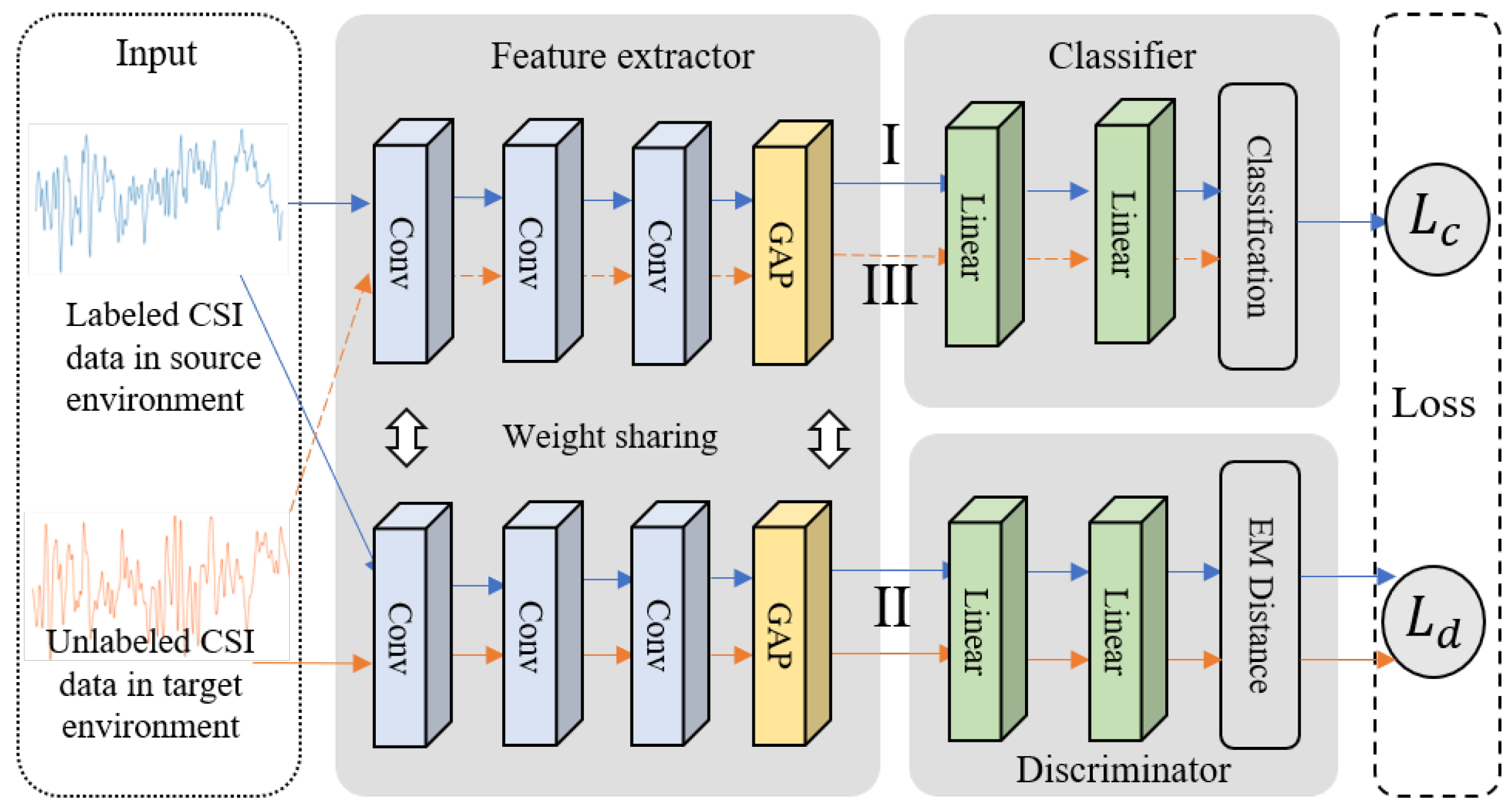
For this stage, we develop an HAR adversarial network. Specifically, we introduce a discriminator module into the basic recognition network (BRN), which consists of a feature extractor and a classifier. The goal is to measure the distance between action features from the source and target environments, and by introducing a maximum–minimum learning strategy, guide the feature extractor to map actions from both environments to a latent space where features are more independent of environmental changes. In this space, the action feature distance between the source and target environments is minimized. This leads to more robust recognition performance in the target environment. The structure of the HAR adversarial network is shown in Figure 10.
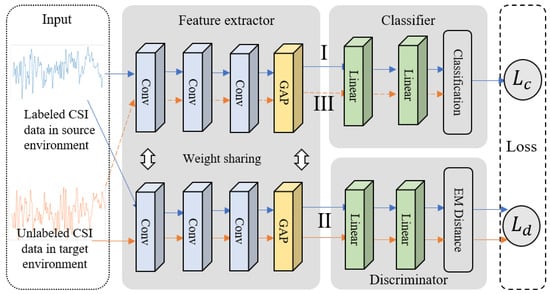
Figure 10.
Structure of the HAR adversarial network, including the feature extractor, classifier, and discriminator.
The BRN is a 1D CNN, with the input being 1D action fragments. To ensure effective input, we normalize the action clips to 1000 frames using an interpolation algorithm. Here, we adopt a classic one-dimensional fully convolutional network (FCN) [41] as the backbone of our BRN. In this structure, we consider the fully connected layers as the classifier, while all layers preceding the fully connected layers serve as the feature extractor. Specifically, the feature extractor consists of three convolutional layers with Rectified Linear Unit (ReLU) activation functions, with each convolutional layer followed by a batch normalization operation. After that, global average pooling (GAP) is utilized to reduce the parameters in the deep model. The first convolutional layer consists of 128 convolutional kernels with a length of 8, the second layer has 256 kernels with a length of 5, and the third layer consists of 128 kernels with a length of 3. The classifier is a fully connected layer whose number of neurons is equal to the number of action classes.
As with general deep learning-based HAR approaches, we optimize the BRN utilizing labeled action samples given in the source environment by minimizing the cross-entropy loss, which corresponds to process I in Figure 10. The cross-entropy loss can be expressed as
where and are the feature extractor and the classifier of the BRN, respectively. is the paired action data and label sample from the labeled source environment dataset , is the indicator function, and K is the number of action classes.
Due to the distribution shift in the action data between the source and target environments, the BRN may not effectively fit the action features of the target environment. To measure the distribution distance between the source environment action features extracted by the BRN and those of the target environment, we introduce a discriminator module after the feature extractor. Given that and represent the feature distribution of the source environment and the target environment, respectively, the EMD between them can be defined as
where denotes the set of all joint distributions whose marginals are and . represents the optimal transport plan that can transform the distribution into distribution with the minimum ‘cost’. With the Kantorovich–Rubinstein duality theorem [42], Equation (8) can be rewritten as
This means that for the parameterized family of functions that are all 1-Lipschitz, we can approximate the by solving the following problem:
With the powerful nonlinear fitting ability of deep learning, we design a deep neural network as the discriminator to approximate the fitting function . To make the designed satisfy the Lipschitz constraint, [43] proposed clipping the discriminator parameters to a fixed range, which may cause gradient vanishing or exploding. We follow [44] to develop a gradient penalty constraint to solve this problem, so the EMD can be further estimated by maximizing the following:
where is the discriminator function, is the action sample from the labeled source environment dataset , and is the action sample from the unlabeled target environment dataset . The first two terms are the original EMD loss , the last term is the gradient penalty constraint , is the random sample along the straight line between the feature distribution pairs of the source environment and the target environment, and is a balance coefficient.
After optimizing the discriminator by maximizing , we can fix the parameters of the discriminator, minimize the loss, and optimize the parameters of the feature extractor through backpropagation. This aims to guide the feature extractor to map the source and target environment action samples to a latent space with a smaller feature distribution EMD distance. By iterating this optimization process, the feature extractor is expected to extract more environment-invariant action features. This process can be expressed as a min–max problem and is illustrated in process II in Figure 10.
where and are the parameters of the feature extractor and the discriminator.
By combining all the above losses, we can obtain the final objective:
where is the parameters of the classifier and is a hyperparameter. The optimization details of this stage are shown in Algorithm 1.
Since the above maximum–minimum learning strategy ensures the transferability of the features extracted by the feature extractor in the BRN, the classifier can be directly applied to action recognition in the target environment. This is shown in process III in Figure 10.
4.3.2. Self-Training Stage
In general, high-precision recognition performance relies on more effective labeled data to optimize the network. By effectively narrowing the distance between action features in the source and target environments through adversarial training, more action samples in the target environment can be effectively recognized and distinguished, providing more stable and accurate pseudo-label information. Inspired by self-training techniques, a form of semi-supervised learning, we propose a self-training strategy that effectively leverages the pseudo-label information of unlabeled action samples in the target environment and conducts iterative optimization to achieve high-performance recognition in the target environment.
Given the target environment dataset , we can get the pseudo-labels after the adversarial training stage.
where denotes the softmax probability of sample belonging to the k-th class output by the classifier.
| Algorithm 1 The optimization algorithm for the adversarial training stage |
Require: The labeled source action dataset, the unlabeled target action dataset, the hyperparameter , the coefficient , and the Adam parameters .
|
Since the pseudo-labels are noisy, samples with larger prediction confidence are considered more likely to be correctly predicted. In practice, samples whose prediction confidence is higher than a given threshold are accounted for in pseudo-label retraining.
However, this threshold-based approach may lead to a class imbalance issue in action samples, with some classes being more easily predicted with high confidence by the network, while others may struggle to reach the set confidence threshold. This may lead to network degradation. This paper proposes a simple and effective method to avoid this issue. The process is designed as follows.
First, we count the number of pseudo-labeled action samples for each class in the target environment to get the set and identify the minimum value n in the set.
where the is the minimum function. Then, we sort the action samples of each class in descending order according to their prediction confidence.
where the is the sorted action sample index set for each class and is the sorting function. Finally, we select the first n samples for each action class as the reliably predicted action samples in . To expand the amount of data and thus ensure recognition performance, we mix these samples with the action samples from the source environment training dataset to form the final reliable dataset .
We utilize this dataset for further optimization of the BRN by minimizing the cross-entropy loss.
The above process is iterated until the network converges.
In addition, the problem of the trivial solution often exists in the self-training stage, that is, the network has a tendency to overfit the noisy pseudo-labels, reducing recognition performance [45]. To avoid this problem, we propose a simple but effective solution that checks the predicted sample number of all classes in each self-training epoch. When the ratio of the number of samples in the class with the fewest identified pseudo-labels to the number in the class with the most identified pseudo-labels falls below 0.1, it indicates that the class balance is severely disrupted, causing the self-training epoch to deviate from the correct optimization path. We suspend the optimization of the network parameters during this epoch until the class balance is restored. The optimization pseudo-code of the self-training stage is illustrated in Algorithm 2.
| Algorithm 2 The optimization algorithm for the self-training stage |
Require: The unlabeled target action dataset , the labeled source action dataset , , the Adam parameters , , .
|
5. Experimental Results and Discussion
5.1. Implementation Details
Optimization details: The supplementary configurations of the CHARS were as follows: We utilized a computer server equipped with 12 vCPU Intel(R) Xeon(R) Platinum 8255C CPUs @ 2.50 GHz and an NVIDIA RTX 2080Ti graphics card, and the PyTorch 1.9.0 deep learning platform to implement and evaluate our proposed CHARS. The discriminator consisted of two fully connected layers with sizes of 120 and 1, and a ReLU nonlinear activation layer. The network was trained for 400 epochs in the first stage and 140 epochs in the second stage, with = 0.00001, starting at 0.001 to speed up training and gradually decreasing by 1/10 every 100 epochs for better convergence, and = 0.0001. The batch size was set to 10, and the Adam algorithm was used to optimize the network, with , = 0.9 and , = 0.999.
Environment setup: To evaluate the adaptability of the proposed CHARS in the target environments, we selected the CSI data from —among the four measured environments—as the source environment, as it provided sufficient labeled samples to support supervised learning. In contrast, the CSI data from , , and were used as the target environments and were unlabeled, making them challenging for accurate recognition. For instance, implies that the network trained on was transferred and adapted to . In this manner, three environmental adaptation scenarios, namely , , and , were utilized to validate the performance of the proposed method across different distribution gaps. In our experiment, 30 samples for each action were chosen for the training set, 5 for the validation set, and 15 samples for the testing set. Only the training set was used for model parameter optimization, while the test set was used to evaluate the HAR performance. It is worth noting that, within the training set, only the samples from the source environment were labeled.
Evaluation metrics: We used the confusion matrix and accuracy to evaluate the HAR performance. Assuming there are K action classes, for each action class in the HAR task, the element of the confusion matrix M represents the percentage of samples that actually belong to class but are predicted as class , relative to the total number of samples in the actual class . This can be formulated as
Therefore, the HAR confusion matrix in our work can be represented as
Accuracy is a common metric used to measure the overall action classification performance of HAR. It is defined as the ratio of correctly classified samples to the total number of samples. The formula is as follows:
5.2. Feasibility Evaluation
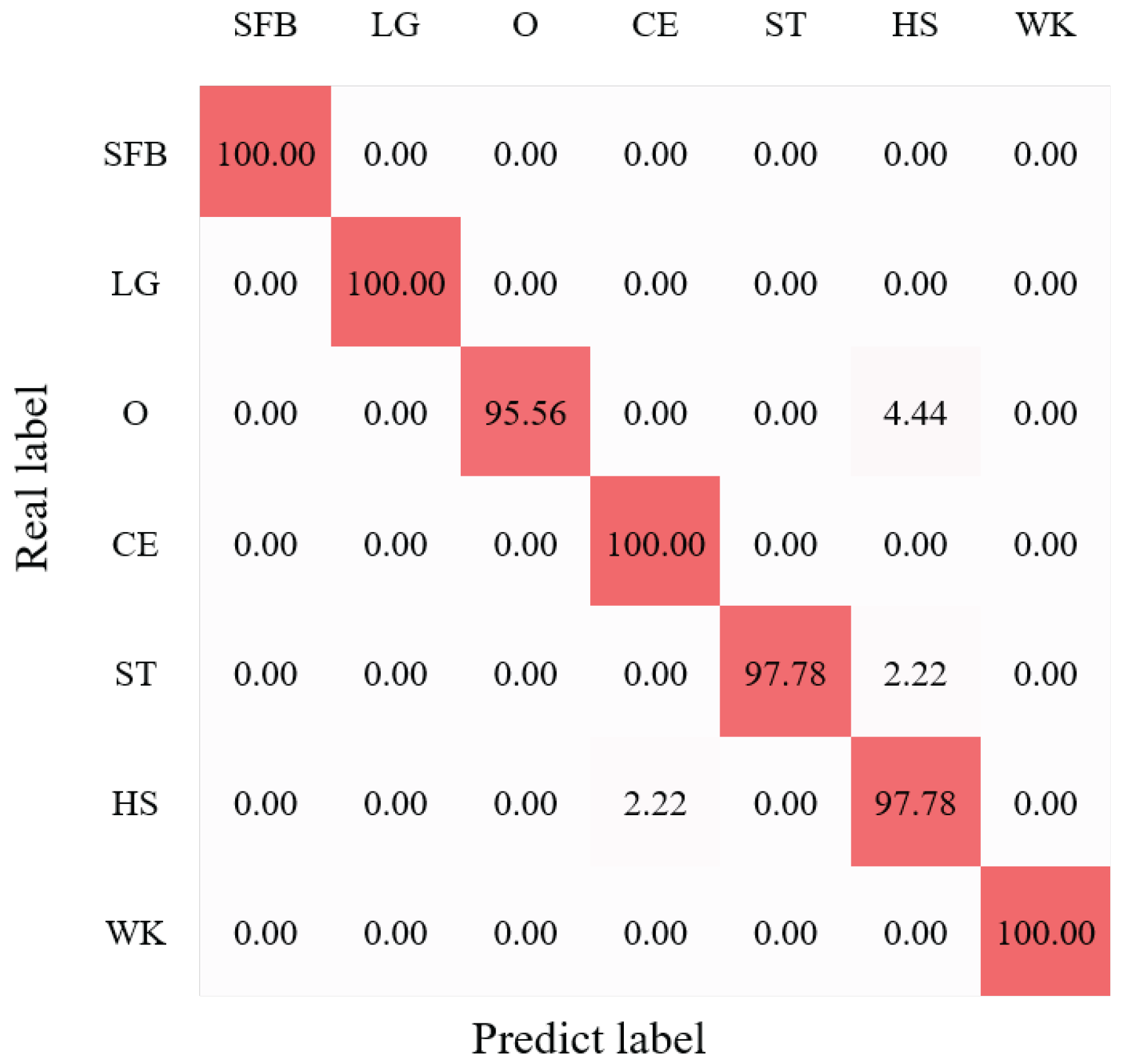
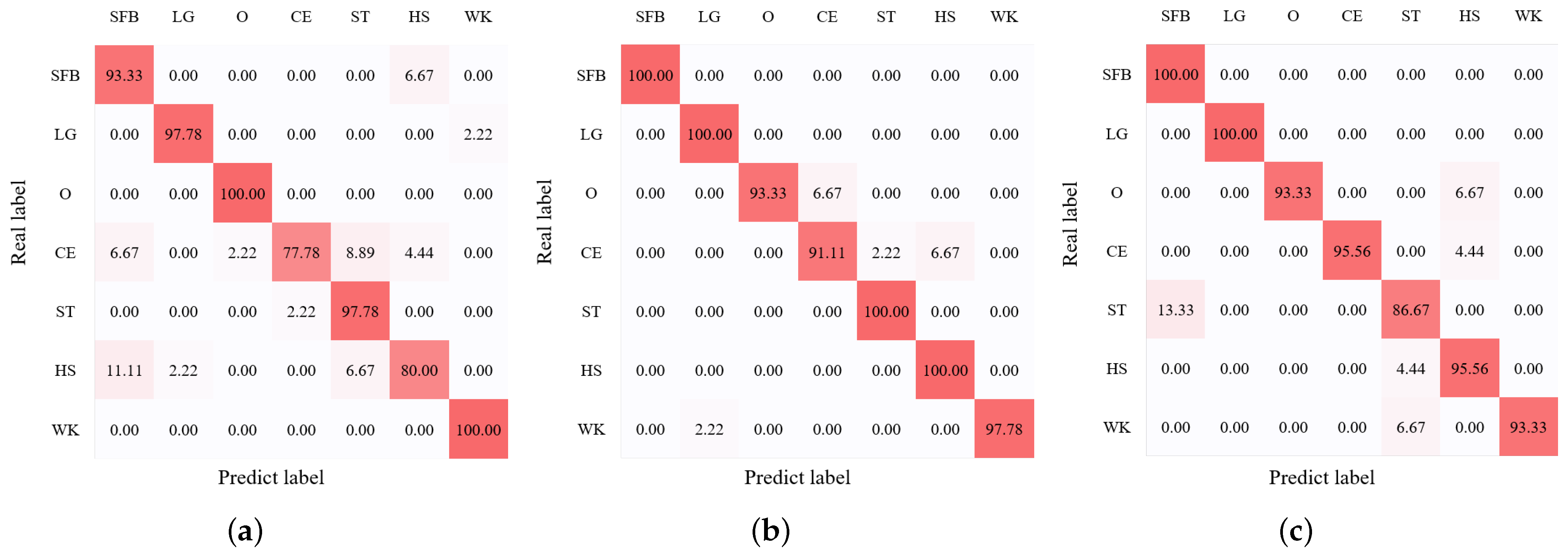
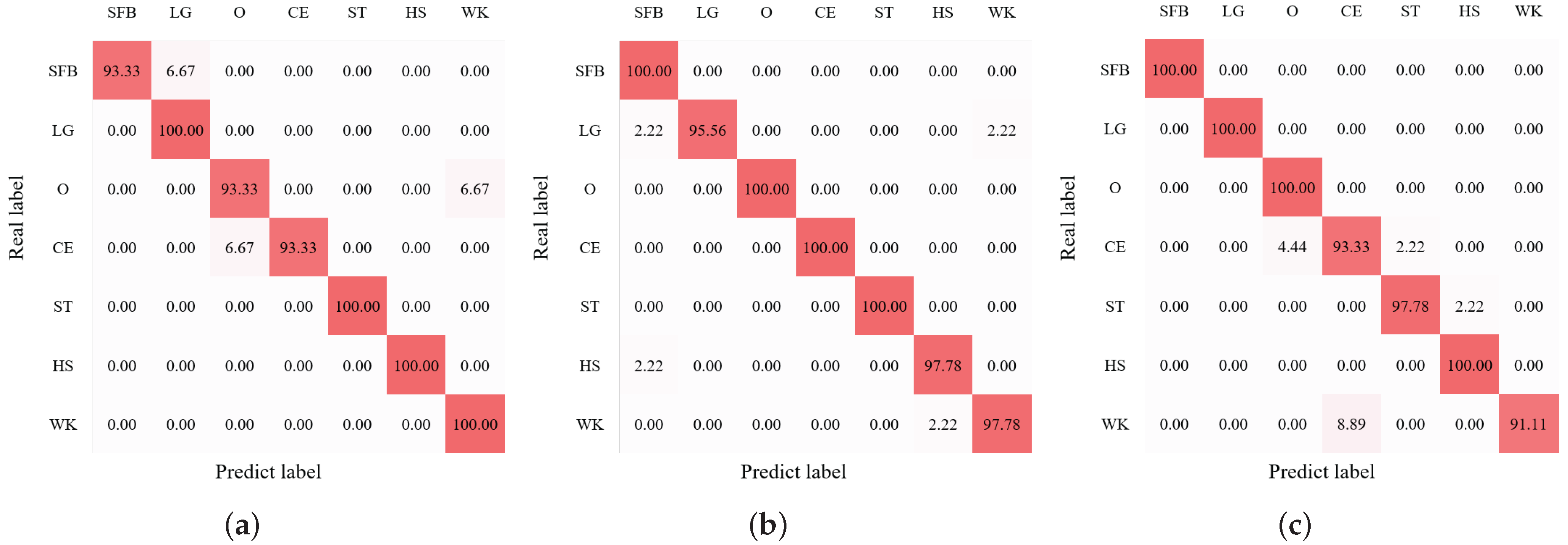
We first conducted the HAR experiments with our BRN of the CHARS in the source environment. The average HAR result is shown in Figure 11, where we can observe that the average recognition accuracy of seven action classes reached 98.73%. In addition, the performance of all action classes exceeded around 95%, and the actions ’SFB’, ’LG’, and ’WK’ even achieved 100% recognition accuracy, showing the effectiveness and good performance of the BRN. We then evaluated the HAR performance in the target environments. Figure 12a–c present the confusion matrices of HAR accuracy in target environments , , and , respectively. Most action classes in all target environments achieved recognition accuracies above 90%.
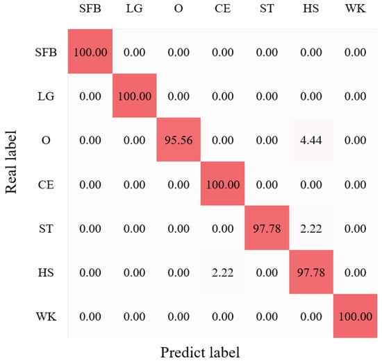
Figure 11.
HAR accuracy (%) confusion matrix of the source environment . The darker the color, the higher the recognition rate.
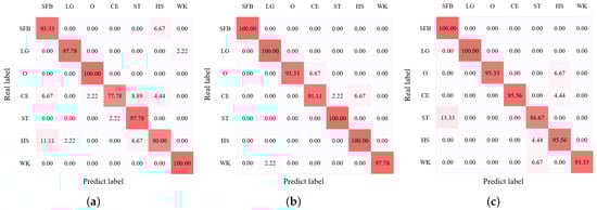
Figure 12.
HAR accuracy (%) confusion matrix of the target environment. (a) , (b) , (c) .
We compared the cross-environment HAR performance of the CHARS in the target environment with that of other representative methods. The results are shown in Table 1. These methods included traditional machine learning, deep learning, and classic cross-domain methods. For traditional machine learning methods, such as K-nearest neighbors (KNN) and SVM, we followed a similar approach to [46], in which HAR is performed by extracting statistical features from action samples, including energy, maximum value, mean value, standard deviation, kurtosis, and skewness. These methods exhibited subpar HAR performance across all target environments, primarily due to the limitations of machine learning algorithms in feature extraction and the differences in action data distribution across different environments. For the deep learning methods, we utilized the popular transformer [29] and CNN models, which are referred to as the BRN in our work, to perform cross-environment HAR. We found that the deep learning approaches demonstrated better HAR performance than the machine learning methods in the target environment due to their powerful feature extraction capabilities. However, they still fell short of achieving reliable cross-environment HAR. For classic cross-domain methods, we primarily considered the EI [36] framework and the Transfer [34]-based method. EI is the most classic DA-based cross-environment HAR method, which introduces a domain discriminator in the multi-class classification network to learn domain representation and eliminates domain-related features extracted by the feature extractor by maximizing the domain label loss to learn transferable action features. The Transfer-based method designs a spatiotemporal model combining a CNN and Bi-LSTM and adopts the transfer learning method. By collecting several labeled samples in the target environment, the pre-trained model parameters in the source environment were optimized to learn the target environment-specific action features, enabling reliable HAR performance in the target environment. In this work, we followed the setup in [34] by collecting five labeled action samples from the volunteers for each action in every target environment. These samples were used for transfer learning from the source environment’s pre-trained model. Compared to traditional machine learning and deep learning methods, these cross-domain methods fully accounted for the feature learning issues in the target environment, resulting in better HAR performance in the target environment.

Table 1.
Comparison of HAR accuracy (%) in the target environment across different methods.
Nonetheless, our CHARS achieved superior performance thanks to its strategy of extracting environment-independent action features and further mining the action pseudo-label information from the target environment. This enabled thorough learning of the action features in the target environment, leading to a significant improvement in cross-environment HAR.
5.3. Module Study
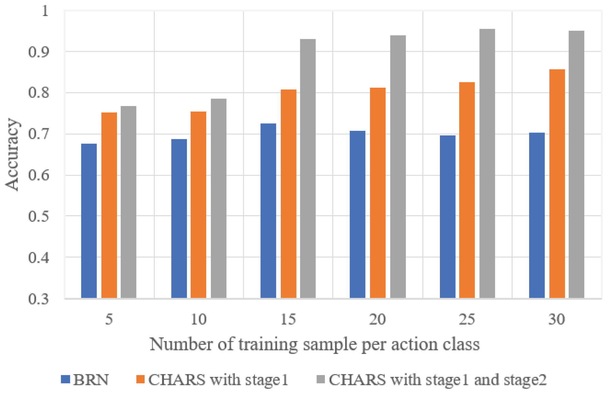
We conducted an ablation study to validate the effectiveness of each stage in the CHARS. The HAR performance of different configurations is shown in Table 2. “CHARS with Stage 1” refers to the introduction of adversarial training based on the BRN to learn environment-independent action features, while “CHARS with Stage 2” represents the use of the proposed self-training strategy to mine the pseudo-label information from the target environment. “CHARS with Stage 1 and Stage 2” represents the full two-stage optimization method. The results indicate that the CHARS with both Stage 1 and Stage 2 outperformed the BRN. In addition, the HAR performance of the two-stage optimization method reached an optimal level of 94.92%, significantly surpassing the performance of the CHARS when using only Stage 1 or Stage 2 independently. This result highlights the effectiveness of incorporating both stages in the optimization strategy.
Table 2.
Comparison of HAR accuracy (%) with different stages of the CHARS.
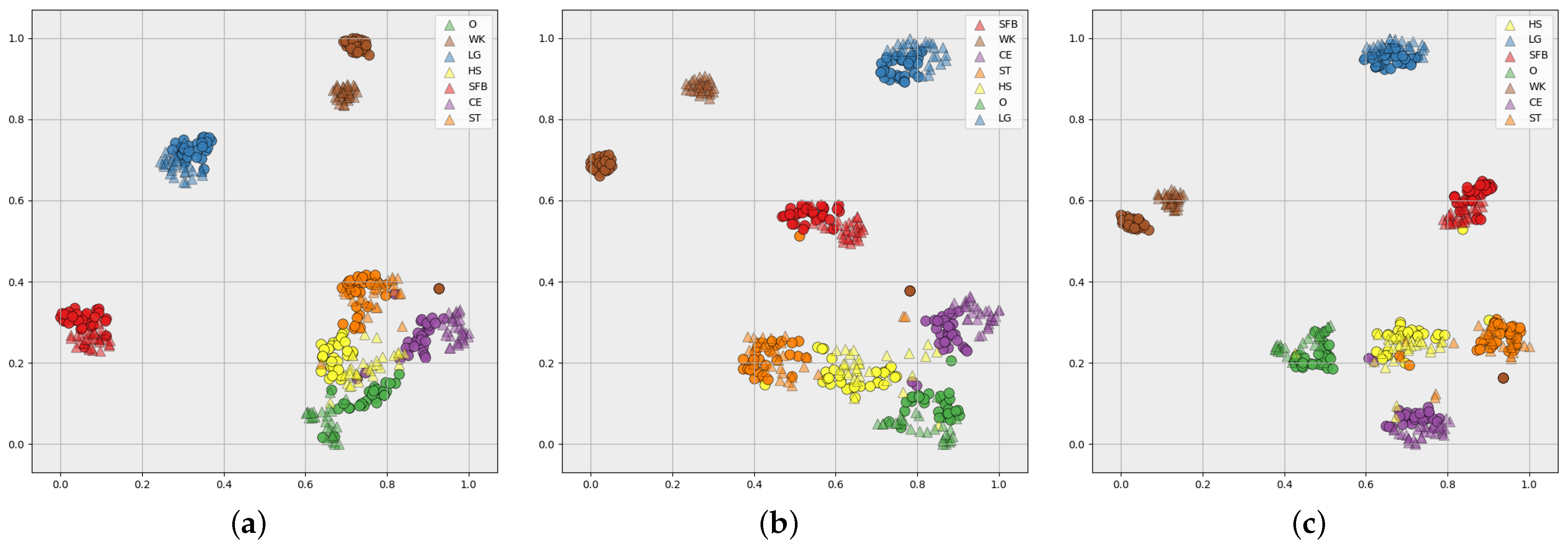
Figure 13 illustrates the visualization feature space in different stages of the CHARS using t-SNE [47] for the source environment and the target environment . The triangular color blocks represent the action features in the source environment, and the circular color blocks represent the action features in the target environment. Different colors represent the different action classes. Figure 13a–c show the feature maps extracted by the BRN, the CHARS with Stage 1, and the CHARS with Stage 1 and Stage 2, respectively. We can observe in Figure 13a that there is a larger gap between some of the same action class features in the source environment and the target environment than between different classes. For example, for ’O’ and ’HS’, ’O’ in the target environment is closer to ’HS’ in the source environment, making recognition ineffective. In addition, different classes of action features, such as ‘O’, ‘ST’, ‘CE’, and ‘HS’, are confused together and difficult to distinguish effectively. This phenomenon illustrates the limitations of the source-environment-optimized recognition network for target-environment HAR. Figure 13b shows that the action features in the target environment and the source environment are better fused, as the distance between the same action category is smaller, demonstrating that the proposed adversarial training strategy can effectively extract the environment-independent action features. However, there still exists the problem of unclear boundaries between some different action classes, such as ‘ST’ and ‘HS’. In Figure 13c, the features of the same action class exhibit better aggregation, and the boundaries between different action classes are also more obvious, validating the effectiveness of the self-training stage.
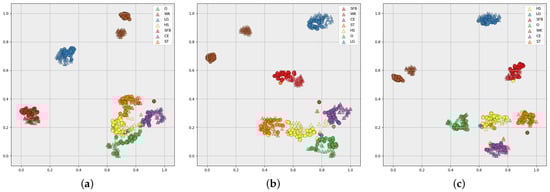
Figure 13.
Visualization feature space of (a) BRN, (b) CHARS with Stage 1, and (c) CHARS with Stage 1 and Stage 2, for the source environment and the target environment . The triangular and circular blocks represent the feature samples in and , respectively, with different-colored blocks indicating different action classes.
We analyzed the impact of using the threshold-based sample selection strategy in Stage 2 of the CHARS on HAR performance in the target environment, keeping the other configurations invariant. Table 3 presents the HAR accuracy under different threshold settings. The threshold-based method did not yield optimal recognition performance, which can be attributed to the class imbalance it introduced. Since the prediction confidence for certain action samples was significantly higher than that for others, the fixed-threshold approach made these action samples more likely to be selected, thus leading to class imbalance, which directly contributed to network degradation.
Table 3.
HAR accuracy (%) with the threshold-based sample selection strategy in Stage 2.
Table 4 shows the impact of mixing source environment data into the generated reliable dataset in Stage 2 on target environment HAR performance. CHARS* represents the absence of source environment data. We can see that this led to a decrease in HAR recognition accuracy of about 1.4 %, which may be because the mixed training dataset greatly increased the number of action samples, thereby helping to learn general action features that are beneficial for HAR.
Table 4.
Comparison of HAR accuracy (%) in the target environment across different methods.
5.4. Robustness Evaluation
We evaluated the impact of the number of action samples on the HAR performance in the target environment. The average HAR performance of all target environments is shown in Figure 14, where the horizontal axis represents the number of samples of each action class in all environments. It can be seen that as the number of action samples increases, the HAR accuracy shows an overall upward trend, which is consistent with our expectations; that is, a larger number of samples helps to better learn action features, thus enhancing HAR performance.
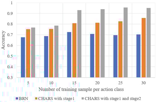
Figure 14.
HAR accuracy under different numbers of training samples in the target environment.
To verify the robustness and generalization of the proposed CHARS, we changed the configurations of the source environment and the target environment and verified the HAR accuracy in these environments. That is, , , and were each set as the source environment in turn, and the remaining environments were set as the target environments to perform cross-environment HAR. Figure 15a–c show the HAR confusion matrix of the source environment with , , and as the source environment. We can observe that the CHARS achieved reliable recognition performance for all action classes in all source environments. When the source environment was , the HAR accuracy in the source environment achieved 97.14%. When the source environment was , the HAR accuracy in the source environment reached 98.73%. When the source environment was , the HAR accuracy in the source environment was 97.46%. The target environment HAR performance is shown in Table 5, where ’’ indicates the average HAR accuracy of the target environment when was the source environment and , , and were the target environments. We can see that the proposed CHARS achieved better recognition performance than the baseline across all scenarios, demonstrating the robustness of CHARS.

Figure 15.
The HAR accuracy (%) confusion matrix of the source environment when (a) , (b) , (c) , as the source environment.
Table 5.
HAR accuracy (%) under different source environment and target environment configurations.
Table 6 provides a detailed summary of the HAR performance in target environments under all cross-environment HAR configurations, where the row index represents the source environment and the column index represents the target environment. The elements in the table represent the HAR accuracy of the target environment when the row-indexed environment is used as the source environment. It can be observed that in the vast majority of cross-environment HAR configurations, the HAR in the target environments achieved reliable performance, demonstrating the effectiveness of the proposed CHARS.
Table 6.
The detailed HAR accuracy (%) of each source environment and target environment configuration.
We further validated the effectiveness of our method on a broader dataset by conducting experiments in three increasingly complex environments: a living room (#1), a bedroom (#2), and a bathroom (#3). We recruited different volunteers and had them perform the same five action categories—falling, picking up, sitting down, standing up, and walking—in different rooms. These experimental environments were more confined, cluttered, and subject to stronger interference. For each environment, we designated one as the source environment and the others as target environments for validation. As shown in Table 7, “#1 → #2 / #3” indicates that #1 was the source environment, and #2 and #3 served as target environments, respectively. The results demonstrate that our method consistently achieved notable performance improvements in the target environments, exhibiting even greater robustness in more challenging settings. We also compared our proposed method with the most relevant baseline (EI), where actions in target environments are unlabeled, as well as with the popular and widely adopted transformer architecture. The experimental results demonstrate the superior effectiveness and generalization ability of our approach.
Table 7.
HAR accuracy (%) on the complex dataset with the living room, bedroom, and bathroom.
We also validated our method on public datasets. In particular, we chose the MultiEnv dataset [48], which contains three environments: (1) a laboratory under line-of-sight (LOS) conditions, (2) a hallway under line-of-sight (LOS) conditions, and (3) a non-line-of-sight (NLOS) room. This dataset contains samples from more than ten action categories collected from several volunteers. We used five action categories, including ’picking a pen up from the ground’, ’falling down’, ’standing still’, ’lying down’, and ’turning’, for the experiments. The experimental results are shown in Table 8. The experiment further verified the effectiveness of this method in improving cross-environment recognition performance.
Table 8.
HAR accuracy (%) on the MultiEnv dataset.
6. Conclusions
In this paper, we propose CHARS, a cross-environment HAR system, to address the widespread problem of poor cross-environment generalization performance in device-free HAR tasks. In this system, a two-stage optimization method is proposed to achieve better cross-environment HAR performance. In the first stage, an adversarial training strategy is used to reduce the feature distribution distance between the source and target environment so as to extract more environment-independent action features. The second stage is based on the self-training strategy, using the target environment action pseudo-label information to further optimize the recognition performance of the recognition network in the target environment iteratively. In this paper, we conduct extensive experiments in different environments. The experimental results show that the algorithm in this paper can achieve reliable recognition accuracy in the target environment and has good robustness in different configurations.
7. Limitations and Future Work
Although our proposed CHARS system has achieved Wi-Fi-based cross-environment HAR, several challenges remain to be addressed. For instance, this work primarily focuses on cross-environment HAR across different sensing scenarios, without fully considering other factors that could impact signal transmissions, such as variations in human states (e.g., changes in body orientation and initial pose), which can further influence the generalization performance of the sensing system to some extent. In future work, we will fully consider the aforementioned influencing factors and conduct large-scale cross-environment HAR research on more extensive datasets with stronger generalization capabilities. We hope this will effectively advance Wi-Fi-based HAR research and better meet the demands of the real consumer market.
Author Contributions
Data curation, S.Z.; Formal analysis, X.D.; Funding acquisition, Y.Z., H.J., and T.J.; Methodology, S.Z.; Resources, T.J.; Supervision, T.J.; Validation, S.Z.; Visualization, S.Z.; Writing—original draft preparation, S.Z.; Writing—review and editing, Y.Z., H.J., X.D., and T.J. All authors have read and agreed to the published version of the manuscript.
Funding
This work was supported by the National Natural Science Foundation of China under grants 62201061, 62071061, and 62301067, and in part by the China Postdoctoral Science Foundation 2023M740340.
Data Availability Statement
Data sharing is not applicable to this article.
Conflicts of Interest
The authors declare no conflicts of interest.
References
- Chen, Y.; Qiu, W.; Computers, S.O. Survey of human action recognition algorithm based on vision. Appl. Res. Comput. 2019, 36, 1927–1934. [Google Scholar]
- Zhang, H.B.; Zhang, Y.X.; Zhong, B.; Lei, Q.; Yang, L.; Du, J.X.; Chen, D.S. A comprehensive survey of vision-based human action recognition methods. Sensors 2019, 19, 1005. [Google Scholar] [CrossRef] [PubMed]
- Abdel-Salam, R.; Mostafa, R.; Hadhood, M. Human Activity Recognition Using Wearable Sensors: Review, Challenges, Evaluation Benchmark. In International Workshop on Deep Learning for Human Activity Recognition, Proceedings of the Second International Workshop, DL-HAR 2020, Kyoto, Japan, 8 January 2021; Springer: Singapore, 2021. [Google Scholar]
- Liu, J.; Liu, H.; Chen, Y.; Wang, Y.; Wang, C. Wireless Sensing for Human Activity: A Survey. IEEE Commun. Surv. Tutor. 2019, 22, 1629–1645. [Google Scholar] [CrossRef]
- Lu, S.; Liu, F.; Li, Y.; Zhang, K.; Huang, H.; Zou, J.; Li, X.; Dong, Y.; Dong, F.; Zhu, J.; et al. Integrated sensing and communications: Recent advances and ten open challenges. IEEE Internet Things J. 2024, 11, 19094–19120. [Google Scholar] [CrossRef]
- Zou, H.; Yang, J.; Zhou, Y.; Xie, L.; Spanos, C.J. Robust WiFi-Enabled Device-Free Gesture Recognition via Unsupervised Adversarial Domain Adaptation. In Proceedings of the 27th International Conference on Computer Communication and Networks (ICCCN), Hangzhou, China, 30 July–2 August 2018; pp. 1–8. [Google Scholar] [CrossRef]
- Guo, Z.; Xiao, F.; Sheng, B.; Fei, H.; Yu, S. WiReader: Adaptive Air Handwriting Recognition Based on Commercial WiFi Signal. IEEE Internet Things J. 2020, 7, 10483–10494. [Google Scholar] [CrossRef]
- Zhong, Y.; Yang, Y.; Zhu, X.; Huang, Y.; Dutkiewicz, E.; Zhou, Z.; Jiang, T. Impact of Seasonal Variations on Foliage Penetration Experiment: A WSN-Based Device-Free Sensing Approach. IEEE Trans. Geosci. Remote Sens. 2018, 56, 5035–5045. [Google Scholar] [CrossRef]
- Zhong, Y.; Wang, J.; Wu, S.; Jiang, T.; Huang, Y.; Wu, Q. Multilocation human activity recognition via MIMO-OFDM-based wireless networks: An IoT-inspired device-free sensing approach. IEEE Internet Things J. 2020, 8, 15148–15159. [Google Scholar] [CrossRef]
- Regani, S.D.; Wu, C.; Wang, B.; Wu, M.; Liu, K.J.R. mmWrite: Passive Handwriting Tracking Using a Single Millimeter-Wave Radio. IEEE Internet Things J. 2021, 8, 13291–13305. [Google Scholar] [CrossRef]
- Yu, G.; Ren, F.; Jie, L. PAWS: Passive Human Activity Recognition Based on WiFi Ambient Signals. IEEE Internet Things J. 2017, 3, 796–805. [Google Scholar]
- Abdelnasser, H.; Youssef, M.; Harras, K.A. WiGest: A Ubiquitous WiFi-based Gesture Recognition System. In Proceedings of the IEEE Conference on Computer Communications, Hong Kong, China, 26 April–1 May 2015. [Google Scholar]
- Niu, K.; Zhang, F.; Wang, X.; Lv, Q.; Luo, H.; Zhang, D. Understanding WiFi signal frequency features for position-independent gesture sensing. IEEE Trans. Mob. Comput. 2021, 21, 4156–4171. [Google Scholar] [CrossRef]
- Xiong, Y.; Liu, F.; Cui, Y.; Yuan, W.; Han, T.X.; Caire, G. On the fundamental tradeoff of integrated sensing and communications under Gaussian channels. IEEE Trans. Inf. Theory 2023, 69, 5723–5751. [Google Scholar] [CrossRef]
- Yang, J.; Chen, X.; Zou, H.; Wang, D.; Xie, L. Autofi: Toward automatic wi-fi human sensing via geometric self-supervised learning. IEEE Internet Things J. 2022, 10, 7416–7425. [Google Scholar] [CrossRef]
- Chowdhury, T.Z.; Leung, C.; Miao, C.Y. WiHACS: Leveraging WiFi for human activity classification using OFDM subcarriers’ correlation. In Proceedings of the 2017 IEEE Global Conference on Signal and Information Processing (GlobalSIP), Montreal, QC, Canada, 14–16 November 2018. [Google Scholar]
- Wang, Y.; Liu, J.; Chen, Y.; Gruteser, M.; Yang, J.; Liu, H. E-eyes: Device-free location-oriented activity identification using fine-grained wifi signatures. In Proceedings of the 20th Annual International Conference on Mobile Computing and Networking, Maui, HI, USA, 7–11 September 2014; pp. 617–628. [Google Scholar]
- Pu, Q.; Gupta, S.; Gollakota, S.; Patel, S. Whole-home gesture recognition using wireless signals. In Proceedings of the 19th Annual International Conference on Mobile Computing & Networking, Miami, FL, USA, 30 September–4 October 2013; pp. 27–38. [Google Scholar]
- Yousefi, S.; Narui, H.; Dayal, S.; Ermon, S.; Valaee, S. A survey on behavior recognition using WiFi channel state information. IEEE Commun. Mag. 2017, 55, 98–104. [Google Scholar] [CrossRef]
- Meneghello, F.; Garlisi, D.; Dal Fabbro, N.; Tinnirello, I.; Rossi, M. Sharp: Environment and person independent activity recognition with commodity ieee 802.11 access points. IEEE Trans. Mob. Comput. 2022, 22, 6160–6175. [Google Scholar] [CrossRef]
- Shi, Z.; Zhang, J.A.; Xu, R.; Cheng, Q.; Pearce, A. Towards environment-independent human activity recognition using deep learning and enhanced CSI. In Proceedings of the GLOBECOM 2020-2020 IEEE Global Communications Conference, Taipei, Taiwan, 7–11 December 2020; pp. 1–6. [Google Scholar]
- Shi, Z.; Zhang, J.A.; Xu, R.Y.; Cheng, Q. Environment-robust device-free human activity recognition with channel-state-information enhancement and one-shot learning. IEEE Trans. Mob. Comput. 2020, 21, 540–554. [Google Scholar] [CrossRef]
- Mei, Y.; Jiang, T.; Ding, X.; Zhong, Y.; Zhang, S.; Liu, Y. WiWave: WiFi-based Human Activity Recognition Using the Wavelet Integrated CNN. In Proceedings of the 2021 IEEE/CIC International Conference on Communications in China (ICCC Workshops), Xiamen, China, 28–30 July 2021; pp. 100–105. [Google Scholar]
- Zhang, S.; Jiang, T.; Ding, X.; Zhong, Y.; Jia, H. A Cloud-Edge Collaborative Framework for Cross-environment Human Action Recognition based on Wi-Fi. In Proceedings of the 2023 IEEE/CIC International Conference on Communications in China (ICCC Workshops), Dalian, China, 10–12 August 2023; pp. 1–6. [Google Scholar]
- Ding, X.; Li, Z.; Yu, J.; Xie, W.; Li, X.; Jiang, T. A Novel Lightweight Human Activity Recognition Method via L-CTCN. Sensors 2023, 23, 9681. [Google Scholar] [CrossRef]
- Ding, X.; Jiang, T.; Zhong, Y.; Wu, S.; Yang, J.; Zeng, J. Wi-Fi-based location-independent human activity recognition with attention mechanism enhanced method. Electronics 2022, 11, 642. [Google Scholar] [CrossRef]
- Li, Z.; Jiang, T.; Yu, J.; Ding, X.; Zhong, Y.; Liu, Y. A lightweight mobile temporal convolution network for multi-location human activity recognition based on wi-fi. In Proceedings of the 2021 IEEE/CIC International Conference on Communications in China (ICCC Workshops), Xiamen, China, 28–30 July 2021; pp. 143–148. [Google Scholar]
- Li, Y.; Jiang, T.; Ding, X.; Wang, Y. Location-free CSI based activity recognition with angle difference of arrival. In Proceedings of the 2020 IEEE Wireless Communications and Networking Conference (WCNC), Seoul, Republic of Korea, 25–28 May 2020; pp. 1–6. [Google Scholar]
- Saidani, O.; Alsafyani, M.; Alroobaea, R.; Alturki, N.; Jahangir, R.; Jamel, L. An efficient human activity recognition using hybrid features and transformer model. IEEE Access 2023, 11, 101373–101386. [Google Scholar] [CrossRef]
- Gao, D.; Wang, L. Multi-scale Convolution Transformer for Human Activity Detection. In Proceedings of the 2022 IEEE 8th International Conference on Computer and Communications (ICCC), Chengdu, China, 9–12 December 2022; pp. 2171–2175. [Google Scholar]
- Zhou, Q.; Xing, J.; Yang, Q. Device-free occupant activity recognition in smart offices using intrinsic Wi-Fi components. Build. Environ. 2020, 172, 106737. [Google Scholar] [CrossRef]
- Zhang, Y.; Zheng, Y.; Qian, K.; Zhang, G.; Liu, Y.; Wu, C.; Yang, Z. Widar3. 0: Zero-Effort Cross-Domain Gesture Recognition with Wi-Fi. IEEE Trans. Pattern Anal. Mach. Intell. 2021, 44, 8671–8688. [Google Scholar]
- Wu, X.; Chu, Z.; Yang, P.; Xiang, C.; Zheng, X.; Huang, W. TW-See: Human activity recognition through the wall with commodity Wi-Fi devices. IEEE Trans. Veh. Technol. 2018, 68, 306–319. [Google Scholar] [CrossRef]
- Sheng, B.; Xiao, F.; Sha, L.; Sun, L. Deep spatial—Temporal model based cross-scene action recognition using commodity WiFi. IEEE Internet Things J. 2020, 7, 3592–3601. [Google Scholar] [CrossRef]
- Wang, J.; Zhao, Y.; Ma, X.; Gao, Q.; Pan, M.; Wang, H. Cross-scenario device-free activity recognition based on deep adversarial networks. IEEE Trans. Veh. Technol. 2020, 69, 5416–5425. [Google Scholar] [CrossRef]
- Jiang, W.; Miao, C.; Ma, F.; Yao, S.; Wang, Y.; Yuan, Y.; Xue, H.; Song, C.; Ma, X.; Koutsonikolas, D.; et al. Towards environment independent device free human activity recognition. In Proceedings of the 24th Annual International Conference on Mobile Computing and Networking, New Delhi, India, 29 October–2 November 2018; pp. 289–304. [Google Scholar]
- Han, Z.; Guo, L.; Lu, Z.; Wen, X.; Zheng, W. Deep adaptation networks based gesture recognition using commodity WiFi. In Proceedings of the 2020 IEEE Wireless Communications and Networking Conference (WCNC), Seoul, Republic of Korea, 25–28 May 2020; pp. 1–7. [Google Scholar]
- Halperin, D.; Hu, W.; Sheth, A.; Wetherall, D. Tool release: Gathering 802.11 n traces with channel state information. ACM SIGCOMM Comput. Commun. Rev. 2011, 41, 53. [Google Scholar] [CrossRef]
- Vallejo, Z.; Jacobo, J. PCA. Principal Component Analysis. Pattern Process. Mach. Intell. Div. Res. Note Dra 2012, 2, 704–706. [Google Scholar]
- Yan, H.; Zhang, Y.; Wang, Y.; Xu, K. WiAct: A Passive WiFi-based Human Activity Recognition System. IEEE Sens. J. 2019, 20, 296–305. [Google Scholar] [CrossRef]
- Wang, Z.; Yan, W.; Oates, T. Time series classification from scratch with deep neural networks: A strong baseline. In Proceedings of the 2017 International joint conference on neural networks (IJCNN), Anchorage, AK, USA, 14–19 May 2017. [Google Scholar]
- Villani, C. Optimal Transport: Old and New; Springer: Berlin/Heidelberg, Germany, 2009; Volume 338. [Google Scholar]
- Arjovsky, M.; Chintala, S.; Bottou, L. Wasserstein generative adversarial networks. In Proceedings of the International Conference on Machine Learning, PMLR, Sydney, Australia, 6–11 August 2017; pp. 214–223. [Google Scholar]
- Gulrajani, I.; Ahmed, F.; Arjovsky, M.; Dumoulin, V.; Courville, A.C. Improved training of wasserstein gans. Adv. Neural Inf. Process. Syst. 2017, 30, 5769–5779. [Google Scholar]
- Zhang, P.; Zhang, B.; Zhang, T.; Chen, D.; Wang, Y.; Wen, F. Prototypical pseudo label denoising and target structure learning for domain adaptive semantic segmentation. In Proceedings of the IEEE/CVF Conference on Computer Vision and Pattern Recognition, Virtual, 19–25 June 2021; pp. 12414–12424. [Google Scholar]
- Ding, X.; Jiang, T.; Zhong, Y.; Wu, S.; Yang, J.; Xue, W. Improving WiFi-based human activity recognition with adaptive initial state via one-shot learning. In Proceedings of the 2021 IEEE Wireless Communications and Networking Conference (WCNC), Nanjing, China, 29 March–1 April 2021; pp. 1–6. [Google Scholar]
- Laurens, V.D.M.; Hinton, G. Visualizing Data using t-SNE. J. Mach. Learn. Res. 2008, 9, 2579–2605. [Google Scholar]
- Alsaify, B.A.; Almazari, M.M.; Alazrai, R.; Daoud, M.I. A dataset for Wi-Fi-based human activity recognition in line-of-sight and non-line-of-sight indoor environments. Data Brief 2020, 33, 106534. [Google Scholar] [CrossRef]
Disclaimer/Publisher’s Note: The statements, opinions and data contained in all publications are solely those of the individual author(s) and contributor(s) and not of MDPI and/or the editor(s). MDPI and/or the editor(s) disclaim responsibility for any injury to people or property resulting from any ideas, methods, instructions or products referred to in the content. |
© 2025 by the authors. Licensee MDPI, Basel, Switzerland. This article is an open access article distributed under the terms and conditions of the Creative Commons Attribution (CC BY) license (https://creativecommons.org/licenses/by/4.0/).